Quark pair production in high
energy pA collisions: General features

Abstract

A consistent treatment of both multiple scattering and small $x$ quantum evolution effects on pair production in high energy pA collisions is feasible in the framework of the Color Glass Condensate (CGC) [1]. We first discuss the properties of quark pair production in the classical effective theory where only multiple scattering effects are included. Explicit results are given for pair production as a function of the invariant mass of pairs, the pair momenta, the atomic mass number $A$ and the quark mass. We relate the logarithms that appear in our formulation of pair production to logarithms that appear in the limit of collinear factorization in QCD. Violations of $k_{\perp}$ factorization and medium modifications, as represented by the Cronin effect, are also investigated. We next consider how small $x$ quantum evolution (shadowing) effects modify the results for pair production. In particular, we provide results for the rapidity distribution of pairs and the dependence of the Cronin effect on rapidity. We discuss the dependence of our results on the initial conditions for small $x$ evolution and comment on its implications for pair production at RHIC and the LHC.

1 Introduction

Proton-nucleus collisions provide a laboratory for studying the interaction of colored partons with an extended colored medium. Due to the combined effects of quantum mechanical coherence over extended longitudinal distances, and the QCD evolution of nuclear wave-functions, the parton from the projectile can probe both the density of color charges in the medium, and the multi-parton correlations that are intrinsic to high parton density components of the nuclear wave function. At high energies, the typical momentum transfer from partons in the medium to the probe is no longer soft and is characterized by a semi-hard scale $Q_{s}^{2}\gg\Lambda_{\rm QCD}^{2}$. This scale, termed the saturation scale, is proportional to the density of partons in the transverse radius of the nucleus, and grows with energy [2, 3, 4]. Because the running of the coupling is controlled by this scale, asymptotic freedom tells us that the coupling of the colored partonic probe should be weak and will become weaker at higher energies. Therefore, with some effort, one can hope to learn about the properties of the medium – in the sense that one can compute reliably medium effects on the final state observables that are measured by experiments.

The study of high parton density effects in QCD can be formulated, in weak coupling, as an effective field theory – the Color Glass Condensate (CGC) [5, 6, 7, 8, 9, 10, 11, 12, 13]. The CGC has been widely applied to study gluon and quark production in proton-nucleus collisions-for a review, see ref. [14]. An attractive feature of the CGC effective theory is that one can quantify what one means by dilute or dense scatterers as a function of energy and mass number [15]. What we mean by proton-nucleus collisions specifically, is a systematic expansion of amplitudes to lowest order in the ratio of the saturation momentum of the proton to the typical transverse momentum exchanged by the proton in the reaction ($Q_{s,p}/k_{\perp,p}\ll 1$) and all orders in the ratio of the saturation momentum of the nucleus relative to the momentum exchanged by the nucleus ($Q_{s}/k_{\perp,A}$). At very high energies, or in very forward kinematics (in the fragmentation region of the nucleus), the proton saturation scale can be large. In these kinematics, for fixed impact parameter, proton-nucleus collisions will be indistinguishable from nucleus-nucleus collisions.

For gluon production in proton-nucleus collisions, the cross-section can be expressed in $k_{\perp}$-factorized form as a product of unintegrated $k_{\perp}$-dependent distributions for the proton and the nucleus, convolved with the hard scattering matrix element [16, 17, 18, 19, 20, 15]. For a dilute projectile, such as a proton, the corresponding unintegrated gluon distribution at lowest order is a leading twist quantity which, integrated over $k_{\perp}$, gives the usual leading log collinear gluon distribution. In contrast, the unintegrated gluon distribution of the dense target, the nucleus, contains all twist contributions and has no analogue in the leading twist collinear factorization formalism. In addition, this remarkable factorization is unlikely to hold beyond leading order in the expansion in powers of $Q_{s,p}(x_{p})/k_{\perp,p}$ [21, 22, 23].

It was shown in ref. [1] that $k_{\perp}$-factorization is broken explicitly in pair production at leading order in proton-nucleus collisions. Novel 3-point and 4-point multi-parton (“all twist”) correlation functions appear in the expression for the pair production cross-section. At large transverse momenta, $k_{\perp}\gg Q_{s}$, these expressions simplify [24] and the cross-section smoothly reduces to the $k_{\perp}$-factorization result of Collins and Ellis [25] and Catani, Ciafaloni and Hautmann [26]. The $k_{\perp}$-factorization formalism of these authors has been used in several phenomenological studies of heavy quark production at collider energies [27, 28, 29]. The magnitude of the breaking of $k_{\perp}$-factorization for single quark production was quantified in ref. [30].

In this paper, we shall discuss in detail qualitative features of pair production that follow from the formalism developed in ref. [1]. A full treatment of multiple scattering and quantum evolution effects at high energies requires a computation of the previously mentioned 2-point, 3-point and 4-point correlation functions as a function of $x$, or of the rapidity $Y$ (= $\ln(1/x)$). These can be determined in full generality (including all leading logarithms in $x$) by solving the Balitsky-JIMWLK equations for the small $x$ evolution of multi-parton correlators [31, 32, 33, 34, 35, 36, 37, 38, 8, 9, 10, 11, 12, 13]. This would require an extensive numerical effort – only preliminary studies have been performed in this direction [39]. Nevertheless, a considerable deal can be learnt in certain limits. At large $N$, and for large nuclei, the small $x$ evolution of the 2-point correlators has a closed form expression called the Balitsky-Kovchegov (BK) equation [37, 40, 41]. Numerical solutions of the Balitsky-Kovchegov equation are known in the fixed coupling [42, 43, 44, 45, 46, 47] and running coupling [39, 48] cases. In the large $N$ and large $A$ limit, the 3-point and 4-point correlators also simplify [54, 55, 56, 1] and their evolution in $x$ can be expressed in terms of the solution of the BK equation. These are computed numerically in this paper. We will also study heavy quark production in the McLerran-Venugopalan (MV) model [5, 6, 7], where high parton density effects contributing to multiple scattering are included but those arising from small $x$ evolution are not included. We are thus able to study quantitatively, in these MV and BK “mean field” limits, the interplay of multiple scattering and small $x$ quantum evolution on pair production.

The high parton density effects we discuss here include contributions categorized as “higher twist” in the established language of collinear factorization. These effects are difficult to treat in that framework and therefore a matching of the two formalisms is difficult. However, one can match the two formalisms at large transverse momenta (specifically, when $Q_{s}^{2}\ll p_{\perp}^{2},M^{2}$) where $k_{\perp}$-factorization formalism is recovered. We shall discuss in general how the logarithms that appear in the $k_{\perp}$-factorization framework can be related to DGLAP [57, 58, 59, 60] logarithms that arise in collinear factorization. Similar considerations arose in other specific processes [61, 62, 63, 64].

The formalism discussed here is valid when at least one of the sources is dilute, as in pA collisions. When the dilute source becomes dense (either by increasing the energy of the proton or in a nucleus-nucleus collision), higher order corrections in $Q_{s,p}/k_{\perp}$ contribute significantly. Thus, in particular for nucleus-nucleus collisions, pair production has to be computed numerically; first results were obtained recently [65, 66].

We will not address phenomenological applications of our approach to pair production in pA collisions in this paper. There are interesting results from D-Au collisions at RHIC [67, 68] and in pA collisions at the SPS [69, 70, 71]. Some of this data has been studied previously in models based on the CGC approach [72, 73]. An interesting comparative study of several models of $J/\psi$ production in heavy ion collisions and relevant references can be found in  [74]. We will address the existing data and make predictions for future data on pair production at RHIC and LHC in a follow up to this work [75].

This paper is organized as follows. In section 2, we state the key results obtained in our previous derivation [1] of the pair production and single quark cross-sections. These were derived as a function of the momenta and rapidity of the quark and the anti-quark and we will re-express these in terms of the pair momenta, invariant mass and rapidity. In section 3, we shall discuss the properties of the multi-parton correlators and present results for their evolution as a function of energy in the large $N$ and large $A$ limit. In section 4, we will present results for the pair cross-sections. The results in this section are presented, in the CGC framework, for a) the McLerran-Venugopalan model and b) for the Balitsky-Kovchegov mean field model of the CGC. As mentioned previously, the former is a reasonable model in the kinematic region where multiple scattering effects are important and small $x$ quantum evolution can be neglected. We discuss, in this model, pair distributions as a function of the pair momenta, rapidity and invariant mass. In particular, we show that the behavior of the spectra at large momenta can be understood analytically. The logarithms that appear in these expressions have the same origin as the collinear logs that appear in collinear factorization formalism of perturbative QCD. At smaller momenta, $k_{\perp}$ factorization is broken explicitly. We demonstrate the dependence of this breaking on the invariant mass and momenta of the pair. In the MV model, the saturation scale $Q_{s}$ depends on the size of the nucleus. We study the dependence of the pair cross-sections on $Q_{s}$ and on the quark mass. We next discuss the behavior of these quantities when small x quantum evolution is turned on. These shadowing effects are obtained by computing the rapidity dependence of correlators with the Balitsky-Kovchegov equation. We compute the rapidity distribution and the invariant mass and momentum distribution of pairs. In particular, we study the Cronin effect for quark pairs and its variation as a function of rapidity. We comment on the dependence of the small x quantum evolution on the large $x$ initial conditions. Section 6 summarizes our conclusions.

2 Quark cross-sections

2.1 Generalities

In the CGC formalism, the proton-nucleus collision is described as a collision of two classical fields originating from color sources representing the large $x$ degrees of freedom in the proton and the nucleus. A schematic representation of the collision in this formalism is shown in fig. 1.

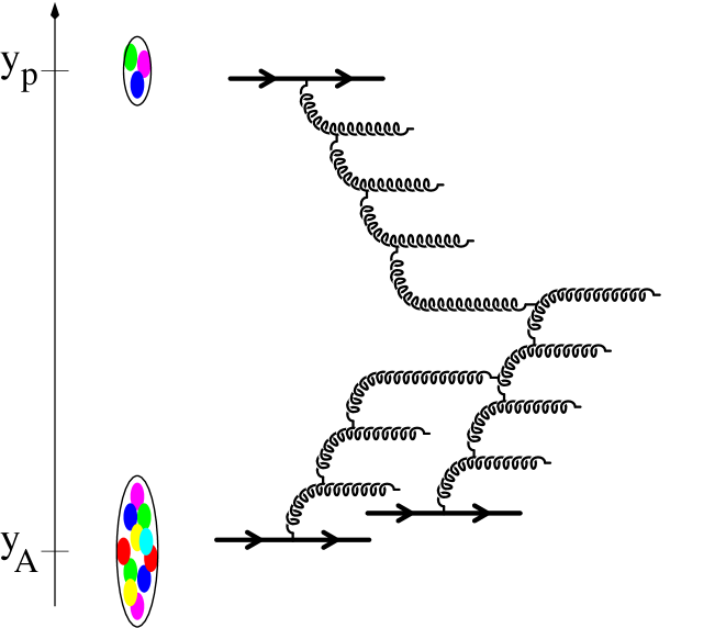
Figure 1: Cartoon representing gluon production in proton-nucleus collisions in the Color Glass Condensate framework.

As suggested by the figure, the color source distribution generating the classical field in each projectile has been evolved from some initial valence distribution at large $x$, in the leading logarithmic approximation in $x$, to the rapidity of interest in the collision. The gauge fields of gluons produced in the collision are determined by solving the Yang-Mills equations

$$[D_{\mu},F^{\mu\nu}]=J^{\nu}\,.$$ (1)

Here $J^{\nu}$ is the color current of the sources, which can expressed at leading order in the sources as

$$J_{a}^{\nu}=g\delta^{\nu+}\delta(x^{-})\,\rho_{p,a}({\boldsymbol{x}}_{\perp})+g\delta^{\nu-}\delta(x^{+})\rho_{{}_{A},a}({\boldsymbol{x}}_{\perp})\,,$$ (2)

where $\rho_{p}$ is the number density of “valence” partons in the proton moving in the $+z$ direction at the speed of light. Likewise, $\rho_{{}_{A}}$ is the number density of “valence” partons in the nucleus moving in the opposite light cone direction. The previous two equations must be supplemented by a gauge fixing condition, and by the covariant conservation of the current :

$$[D_{\nu},J^{\nu}]=0\;.$$ (3)

The latter equation in general implies that eq. (2) for the current receives corrections that are of higher order in the sources $\rho_{p}$ and $\rho_{{}_{A}}$, because of the radiated field. The solution of eqs. (1), (2) and (3) has been determined to all orders in both sources only numerically [22, 23, 76]. To lowest order in the proton source (as appropriate for a dilute proton source) and to all orders in the nuclear source, analytical results are available and an explicit expression for the gauge field to this order, in Lorentz gauge, is given in ref. [15]. The amplitude for pair production to this order is obtained by computing the quark propagator in the background corresponding to this gauge field [1]. The diagrams corresponding to these insertions are shown in fig. 2.

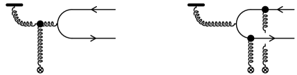
Figure 2: The two types of terms that enter in the $Q\overline{Q}$ production amplitude in pA collisions. The gluon emitted by the proton can either emit the pair after the collision with the nucleus (left diagram) or before colliding with the nucleus (diagram on the right). The black blob denotes multiple scatterings resummed via Wilson lines.

The probability for producing a single $q\bar{q}$ pair in the collision can be expressed as

$$P_{1}[\rho_{p},\rho_{{}_{A}}]=\int\frac{d^{3}{\boldsymbol{q}}}{(2\pi)^{3}2E_{\boldsymbol{q}}}\int\frac{d^{3}{\boldsymbol{p}}}{(2\pi)^{3}2E_{\boldsymbol{p}}}\left|{\cal M}_{{}_{F}}({\boldsymbol{q}},{\boldsymbol{p}})\right|^{2}\;,$$ (4)

where ${\cal M}_{{}_{F}}({\boldsymbol{q}},{\boldsymbol{p}})$ is the amputated time-ordered quark propagator in the presence of the classical field. The argument $[\rho_{p},\rho_{{}_{A}}]$ indicates that this is the production probability in one particular configuration of the color sources. In order to turn this probability into a cross-section, one must first average over the initial classical sources $\rho_{p}$ and $\rho_{{}_{A}}$ respectively with the weights  $W_{p}[x_{p},\rho_{p}],W_{{}_{A}}[x_{{}_{A}},\rho_{{}_{A}}]$ and subsequently integrate over all the impact parameters ${\boldsymbol{b}}$, to obtain,

$$\sigma=\int d^{2}{\boldsymbol{b}}\int[D\rho_{p}][D\rho_{{}_{A}}]\,W_{p}[x_{p},\rho_{p}]\,W_{{}_{A}}[x_{{}_{A}},\rho_{{}_{A}}]P_{1}[\rho_{p},\rho_{{}_{A}}]\;.$$ (5)

This formula incorporates both multiple scattering effects and quantum effects. The multiple scattering effects are in part included in the classical field (the solution of Yang-Mills equations), in part in the propagator of the quark in this classical field, and also in the evolution with $x$ of the source distributions. The quantum effects are included in the evolution of the weight functionals, $W_{p}$ and $W_{{}_{A}}$, of the target and projectile with $x$. The arguments $x_{p}$ and $x_{{}_{A}}$ denote the scale in $x$ separating the large-$x$ static sources from the small-$x$ dynamical fields. In the McLerran-Venugopalan model, the functional $W_{{}_{A}}$ that describes the distribution of color sources in the nucleus is a Gaussian in the color charge density  in $\rho_{{}_{A}}$ [5, 6, 7]. Having a Gaussian distribution of sources, in our framework, is equivalent to the Glauber model of independent multiple scattering [15]. In general, this Gaussian is best interpreted as the initial condition for a non-trivial evolution of $W_{{}_{A}}[x_{{}_{A}},\rho_{{}_{A}}]$ with $x_{{}_{A}}$. This evolution is described by a Wilson renormalization group equation – the JIMWLK equation [31, 32, 33, 34, 35, 36, 37, 38, 8, 9, 10]. We will discuss evolution equations further in the following section.

2.2 Differential pair cross-section

The pair production cross-section, for quarks (anti-quarks) of momenta ${\boldsymbol{q}}_{\perp}$ (${\boldsymbol{p}}_{\perp}$) and rapidities $y_{q}=1/2\ln(q^{+}/q^{-})$ ($y_{p}=1/2\ln(p^{+}/p^{-})$), derived in [1] can be expressed as

$$\frac{d\sigma}{d^{2}{\boldsymbol{p}}_{\perp}d^{2}{\boldsymbol{q}}_{\perp}dy_{p}dy_{q}}=\frac{\alpha_{s}^{2}N}{8\pi^{4}(N^{2}-1)}\int\limits_{{\boldsymbol{k}}_{1\perp},{\boldsymbol{k}}_{2\perp}}\!\!\!\frac{\delta({\boldsymbol{p}}_{\perp}+{\boldsymbol{q}}_{\perp}-{\boldsymbol{k}}_{1\perp}-{\boldsymbol{k}}_{2\perp})}{{\boldsymbol{k}}_{1\perp}^{2}{\boldsymbol{k}}_{2\perp}^{2}}\,\varphi_{p}({\boldsymbol{k}}_{1\perp})$$

$$\qquad\qquad\!\!\!\!\!\times\Bigg{\{}\int\limits_{{\boldsymbol{k}}_{\perp},{\boldsymbol{k}}_{\perp}^{\prime}}\!\!\!\!\!{\rm tr}_{\rm d}\Big{[}(\raise 0.43057pt\hbox{$/$}\kern-5.29999pt\hbox{$q$}\!+\!m)T_{q\bar{q}}(\raise 0.43057pt\hbox{$/$}\kern-6.30005pt\hbox{$p$}\!-\!m)\gamma^{0}T_{q\bar{q}}^{\prime\dagger}\gamma^{0}\Big{]}\phi_{{}_{A}}^{q\bar{q},q\bar{q}}({\boldsymbol{k}}_{2\perp};{\boldsymbol{k}}_{\perp},{\boldsymbol{k}}_{\perp}^{\prime})$$

$$\qquad\qquad\;\;+\int\limits_{{\boldsymbol{k}}_{\perp}}\!{\rm tr}_{\rm d}\Big{[}(\raise 0.43057pt\hbox{$/$}\kern-5.29999pt\hbox{$q$}\!+\!m)T_{q\bar{q}}(\raise 0.43057pt\hbox{$/$}\kern-6.30005pt\hbox{$p$}\!-\!m)\gamma^{0}T_{g}^{\dagger}\gamma^{0}+{\it h.c.}\Big{]}\phi_{{}_{A}}^{q\bar{q},g}({\boldsymbol{k}}_{2\perp};{\boldsymbol{k}}_{\perp})$$

$$\qquad\qquad\qquad+{\rm tr}_{\rm d}\Big{[}(\raise 0.43057pt\hbox{$/$}\kern-5.29999pt\hbox{$q$}\!+\!m)T_{g}(\raise 0.43057pt\hbox{$/$}\kern-6.30005pt\hbox{$p$}\!-\!m)\gamma^{0}T_{g}^{\dagger}\gamma^{0}\Big{]}\phi_{{}_{A}}^{g,g}({\boldsymbol{k}}_{2\perp})\Bigg{\}}\;.$$ (6)

where we denote

$$T_{q\bar{q}}({\boldsymbol{k}}_{1\perp},{\boldsymbol{k}}_{\perp})\equiv\frac{\gamma^{+}(\raise 0.43057pt\hbox{$/$}\kern-5.29999pt\hbox{$q$}-\raise 0.6458pt\hbox{$/$}\kern-5.29999pt\hbox{$k$}+m)\gamma^{-}(\raise 0.43057pt\hbox{$/$}\kern-5.29999pt\hbox{$q$}-\raise 0.6458pt\hbox{$/$}\kern-5.29999pt\hbox{$k$}-\raise 0.6458pt\hbox{$/$}\kern-5.29999pt\hbox{$k$}_{1}+m)\gamma^{+}}{2p^{+}[({\boldsymbol{q}}_{\perp}\!-\!{\boldsymbol{k}}_{\perp})^{2}+m^{2}]+2q^{+}[({\boldsymbol{q}}_{\perp}\!-\!{\boldsymbol{k}}_{\perp}\!-\!{\boldsymbol{k}}_{1\perp})^{2}+m^{2}]}$$

$$T_{g}({\boldsymbol{k}}_{1\perp})\equiv\frac{\raise 0.6458pt\hbox{$/$}\kern-5.29999pt\hbox{$C$}_{{}_{L}}(p+q,{\boldsymbol{k}}_{1\perp})}{(p+q)^{2}}\;.$$ (7)

Note that $T_{q\bar{q}}^{\prime}\equiv T_{q\bar{q}}({\boldsymbol{k}}_{1\perp},{\boldsymbol{k}}_{\perp}^{\prime})$ and $C_{L}^{\mu}$ is the well-known Lipatov vertex defined as

$$C_{{}_{L}}^{+}(q,{\boldsymbol{k}}_{1\perp})\equiv\frac{-k_{1\perp}^{2}}{q^{-}}+q^{+}\,\,;\,\,C_{{}_{L}}^{-}(q,{\boldsymbol{k}}_{1\perp})\equiv\frac{k_{2\perp}^{2}}{q^{+}}-q^{-}\,\,;\,\,C_{{}_{L}}^{i}(q,{\boldsymbol{k}}_{1\perp})\equiv-2k_{1}^{i}+q^{i}\,,$$ (8)

with ${\boldsymbol{k}}_{2\perp}\equiv{\boldsymbol{q}}_{\perp}-{\boldsymbol{k}}_{1\perp}$.

$\varphi_{p}$ is the unintegrated gluon distribution of the proton and the various $\phi_{{}_{A}}$’s are unintegrated distributions describing the target. As stated previously, we are working to lowest order in the color charge density $\rho_{p}$ of the proton. The proton unintegrated distribution is given by 

$$\varphi_{p}({\boldsymbol{l}}_{\perp})\equiv\frac{\pi^{2}R_{p}^{2}\,g^{2}}{l_{\perp}^{2}}\int_{{\boldsymbol{x}}_{\perp}}e^{i{\boldsymbol{l}}_{\perp}\cdot{\boldsymbol{x}}_{\perp}}\left<\rho_{p}^{a}(0)\rho_{p}^{a}({\boldsymbol{x}}_{\perp})\right>\;.$$ (9)

The corresponding nuclear “unintegrated distributions” are defined to be

$$\phi_{{}_{A}}^{g,g}({\boldsymbol{l}}_{\perp})\equiv\frac{\pi^{2}R_{{}_{A}}^{2}l_{\perp}^{2}}{g^{2}N}\int_{{\boldsymbol{x}}_{\perp}}e^{i{\boldsymbol{l}}_{\perp}\cdot{\boldsymbol{x}}_{\perp}}\,{\rm tr}\,\left<U(0)U^{\dagger}({\boldsymbol{x}}_{\perp})\right>\;,$$

$$\phi_{{}_{A}}^{q\bar{q},g}({\boldsymbol{l}}_{\perp};{\boldsymbol{k}}_{\perp})\equiv\frac{2\pi^{2}R_{{}_{A}}^{2}l_{\perp}^{2}}{g^{2}N}\int_{{\boldsymbol{x}}_{\perp},{\boldsymbol{y}}_{\perp}}\!\!\!\!\!\!\!\!\!\!e^{i({\boldsymbol{k}}_{\perp}\cdot{\boldsymbol{x}}_{\perp}+({\boldsymbol{l}}_{\perp}-{\boldsymbol{k}}_{\perp})\cdot{\boldsymbol{y}}_{\perp})}$$

$$\qquad\qquad\qquad\times{\rm tr}\left<{\widetilde{U}}({\boldsymbol{x}}_{\perp})t^{a}{\widetilde{U}}^{\dagger}({\boldsymbol{y}}_{\perp})t^{b}U_{ba}(0)\right>$$

$$\phi_{{}_{A}}^{q\bar{q},q\bar{q}}({\boldsymbol{l}}_{\perp};{\boldsymbol{k}}_{\perp},{\boldsymbol{k}}_{\perp}^{\prime})\equiv\frac{2\pi^{2}R_{{}_{A}}^{2}l_{\perp}^{2}}{g^{2}N}\int_{{\boldsymbol{x}}_{\perp}^{\prime},{\boldsymbol{y}}_{\perp},{\boldsymbol{y}}_{\perp}^{\prime}}\!\!\!\!\!\!\!\!\!\!e^{i(-{\boldsymbol{k}}_{\perp}\cdot{\boldsymbol{y}}_{\perp}+{\boldsymbol{l}}_{\perp}\cdot({\boldsymbol{y}}_{\perp}-{\boldsymbol{y}}_{\perp}^{\prime})+{\boldsymbol{k}}_{\perp}^{\prime}\cdot({\boldsymbol{y}}_{\perp}^{\prime}-{\boldsymbol{x}}_{\perp}^{\prime}))}$$

$$\qquad\qquad\qquad\times{\rm tr}\left<{\widetilde{U}}(0)t^{a}{\widetilde{U}}^{\dagger}({\boldsymbol{y}}_{\perp}){\widetilde{U}}({\boldsymbol{x}}_{\perp}^{\prime})t^{a}{\widetilde{U}}^{\dagger}({\boldsymbol{y}}_{\perp}^{\prime})\right>\,.$$ (10)

The matrices $U$ are path ordered exponentials along the light cone longitudinal extent corresponding to partonic configurations of the nucleus in the infinite momentum frame:

$$U({\boldsymbol{x}}_{\perp})\equiv{\cal P}_{+}\exp\left[-ig^{2}\int_{-\infty}^{+\infty}dz^{+}\frac{1}{{\boldsymbol{\nabla}}_{\perp}^{2}}\,\rho_{{}_{A}}(z^{+},{\boldsymbol{x}}_{\perp})\cdot T\right]\,,$$ (11)

where the $T^{a}$ are the generators of the adjoint representation of $SU(N)$ and ${\cal P}_{+}$ denotes a “time ordering” along the $z^{+}$ axis. The ${\widetilde{U}}$ have an identical definition, with the generators $T^{a}$ replaced by the generators $t^{a}$ in the fundamental representation of $SU(N)$. We remind the reader that the expectation values $\big{<}\cdots\big{>}$ here correspond to the averages over the sources $\rho_{p}$ in the case of $\varphi_{p}$ and $\rho_{{}_{A}}$ in the case of the $\phi_{{}_{A}}$’s.

In the definition of these distribution functions, the momentum ${\boldsymbol{l}}_{\perp}$ is the total transverse momentum exchanged between the nucleus and the probe (either a gluon or the $Q\overline{Q}$ state), and ${\boldsymbol{k}}_{\perp},{\boldsymbol{k}}^{\prime}_{\perp}$ are the momenta exchanged between the quark and the nucleus. These conventions can be visualized in the diagrams

$$\phi_{{}_{A}}^{g,g}({\boldsymbol{l}}_{\perp}) =$$

$$\phi_{{}_{A}}^{q\bar{q},g}({\boldsymbol{l}}_{\perp};{\boldsymbol{k}}_{\perp}) =$$

$$\phi_{{}_{A}}^{q\bar{q},q\bar{q}}({\boldsymbol{l}}_{\perp};{\boldsymbol{k}}_{\perp},{\boldsymbol{k}}_{\perp}^{\prime}) =$$ (12)

It is transparent that eq. (6) for the pair production cross-section is not in general $k_{\perp}$-factorizable into a simple convolution of unintegrated parton distributions from the proton and the nucleus. While one can still factorize out the proton unintegrated distribution, the nucleus is now represented by the distributions $\phi_{{}_{A}}^{g,g}$, $\phi_{{}_{A}}^{q\bar{q},g}$, and $\phi_{{}_{A}}^{q\bar{q},q\bar{q}}$, which are respectively 2-point, 3-point and 4-point correlators of Wilson lines in the color field of the nucleus. These multi-parton correlation functions contain all twists and are in general rather complicated. They however, in all generality, satisfy the sum rule,

$$\int\limits_{{\boldsymbol{k}}_{\perp},{\boldsymbol{k}}_{\perp}^{\prime}}{\phi_{{}_{A}}^{q\bar{q},q\bar{q}}({\boldsymbol{l}}_{\perp};{\boldsymbol{k}}_{\perp},{\boldsymbol{k}}_{\perp}^{\prime})}=\int\limits_{{\boldsymbol{k}}_{\perp}}{\phi_{{}_{A}}^{q\bar{q},g}({\boldsymbol{l}}_{\perp};{\boldsymbol{k}}_{\perp})}={\phi_{{}_{A}}^{g,g}({\boldsymbol{l}}_{\perp})}\;.$$ (13)

2.3 Leading twist limit

It is illustrative to consider when one recovers $k_{\perp}$-factorization. For Gaussian correlations,

$$\langle\rho_{{}_{A},a}({\boldsymbol{x}}_{\perp})\rho_{{}_{A},a^{\prime}}({\boldsymbol{x}}_{\perp}^{\prime})\rangle=\delta_{aa^{\prime}}\delta({\boldsymbol{x}}_{\perp}-{\boldsymbol{x}}_{\perp}^{\prime})\mu_{{}_{A}}^{2}\;,$$ (14)

where $\mu_{{}_{A}}^{2}=A/2\pi R_{A}^{2}\propto A^{1/3}$. One obtains, in the leading twist approximation (where the path ordered exponentials are expanded to lowest order in $\rho_{{}_{A}}/k_{\perp}^{2}$),

$$\phi_{{}_{A}}^{g,g}({\boldsymbol{k}}_{2\perp})\approx\pi R^{2}\left[{\pi d_{{}_{A}}g^{2}}\frac{\mu_{{}_{A}}^{2}}{{\boldsymbol{k}}_{2\perp}^{2}}\right]\;,$$

$$\phi_{{}_{A}}^{g,q\bar{q}}({\boldsymbol{k}}_{2\perp};{\boldsymbol{k}}_{\perp})\approx\frac{\pi R^{2}}{2}\left[{\pi d_{{}_{A}}g^{2}}\frac{\mu_{{}_{A}}^{2}}{{\boldsymbol{k}}_{2\perp}^{2}}\right](2\pi)^{2}\left[\delta({\boldsymbol{k}}_{\perp})\!+\!\delta({\boldsymbol{k}}_{\perp}\!-\!{\boldsymbol{k}}_{2\perp})\right]$$

$$\phi_{{}_{A}}^{q\bar{q},q\bar{q}}({\boldsymbol{k}}_{2\perp};{\boldsymbol{k}}_{\perp},{\boldsymbol{k}}_{\perp}^{\prime})\approx\pi R^{2}\left[{\pi d_{{}_{A}}g^{2}}\frac{\mu_{{}_{A}}^{2}}{{\boldsymbol{k}}_{2\perp}^{2}}\right]$$

$$\qquad\qquad\times(2\pi)^{4}\Big{[}\frac{C_{{}_{F}}}{N}\left(\delta({\boldsymbol{k}}_{\perp}-{\boldsymbol{k}}_{2\perp})\delta({\boldsymbol{k}}_{\perp}^{\prime}-{\boldsymbol{k}}_{2\perp})+\delta({\boldsymbol{k}}_{\perp})\delta({\boldsymbol{k}}_{\perp}^{\prime})\right)$$

$$\qquad\qquad\qquad+\frac{1}{2N^{2}}\left(\delta({\boldsymbol{k}}_{\perp}-{\boldsymbol{k}}_{2\perp})\delta({\boldsymbol{k}}_{\perp}^{\prime})+\delta({\boldsymbol{k}}_{\perp})\delta({\boldsymbol{k}}_{\perp}^{\prime}-{\boldsymbol{k}}_{2\perp})\right)\Big{]}\;.$$

(15)

We assume here that the nuclei have a large uniform transverse area $\pi R^{2}$. The leading twist expressions for $\phi_{{}_{A}}^{g,q\bar{q}}$ and $\phi_{{}_{A}}^{q\bar{q},q\bar{q}}$ have a simple interpretation. At this order, the probe (gluon or $q\bar{q}$ pair) interacts with the nucleus by a single gluon exchange. The two delta functions in $\phi_{{}_{A}}^{g,q\bar{q}}$ correspond to the gluon being attached to the anti-quark line ($\delta({\boldsymbol{k}}_{\perp})$ – there is no momentum flow from the nucleus to the quark line) or to the quark line ($\delta({\boldsymbol{k}}_{2\perp}-{\boldsymbol{k}}_{\perp})$ – all the momentum from the nucleus flows on the quark line). An identical interpretation holds for the four terms of $\phi_{{}_{A}}^{q\bar{q},q\bar{q}}$. If one substitutes these leading twist approximations in eq. (6), one recovers the leading twist $k_{\perp}$-factorized cross-section for pair production [25, 26, 24].

2.4 Kinematics

We have to specify the multi-parton correlators $\phi_{{}_{A}}^{g,g}({\boldsymbol{l}}_{\perp})$, $\phi_{{}_{A}}^{q\bar{q},g}({\boldsymbol{l}}_{\perp};{\boldsymbol{k}}_{\perp})$, and $\phi_{{}_{A}}^{q\bar{q},q\bar{q}}({\boldsymbol{l}}_{\perp};{\boldsymbol{k}}_{\perp},{\boldsymbol{k}}_{\perp}^{\prime})$ in order to compute the pair production cross-section. The following section will be devoted to a discussion of how one does this. Before proceeding, however, we will first discuss the kinematic variables in terms of which the pair production cross-section is specified.

It is convenient to discuss the properties of the produced pairs in terms of the pair invariant mass $M^{2}$, the pair rapidity $Y$ and the pair transverse momentum ${\boldsymbol{P}}_{\perp}$. These are defined in terms of the momenta and rapidities of the quark and the anti-quark as

$${\boldsymbol{P}}_{\perp} = {\boldsymbol{p}}_{\perp}+{\boldsymbol{q}}_{\perp}$$

$$Y = \frac{1}{2}\ln\left(\frac{p^{+}+q^{+}}{p^{-}+q^{-}}\right)=\frac{1}{2}\ln\left(\frac{\omega_{p}\,e^{y_{p}}+\omega_{q}\,e^{y_{q}}}{\omega_{p}\,e^{-y_{p}}+\omega_{q}\,e^{-y_{q}}}\right)$$

$$M^{2} = \omega_{p}^{2}+\omega_{q}^{2}+2\,\omega_{p}\,\omega_{q}\,\cosh\left(y_{p}-y_{q}\right)-{\boldsymbol{P}}_{\perp}^{2}\;.$$ (16)

Here $\omega_{q}\equiv\sqrt{{\boldsymbol{q}}_{\perp}^{2}+m^{2}}$ and $\omega_{p}\equiv\sqrt{{\boldsymbol{p}}_{\perp}^{2}+m^{2}}$ are the transverse masses of the quark and the anti-quark respectively, and $y_{p}\equiv\ln(p^{+}/p^{-})/2$ and $y_{q}\equiv\ln(q^{+}/q^{-})/2$ are their respective rapidities. We would like to express the cross-section in eq. (6) in terms of the pair kinematical parameters. Firstly, one notices that the cross-section in eq. (6) is expressed in terms of six variables while the pair invariants correspond to four variables. In other words, a given set of kinematical parameters for the pair corresponds to a 2-dimensional manifold in the phase-space of the quark and anti-quark. One writes

$$\frac{d\sigma}{dM^{2}\,d^{2}{\boldsymbol{P}}_{\perp}\,dY}=\!\!\!\int\limits_{0}^{\sqrt{\frac{M^{2}}{4}-m^{2}}}\!\!\!\!\!\!d{\tilde{q}}\int\limits_{0}^{2\pi}d\phi\;\frac{{\tilde{q}}\gamma_{x}}{\omega_{p}\,\omega_{q}\,|\sinh\left(y_{p}-y_{q}\right)|}\;\frac{d\sigma}{d^{2}{\boldsymbol{p}}_{\perp}dy_{p}\,d^{2}{\boldsymbol{q}}_{\perp}dy_{q}}\;.$$ (17)

In the $Q\overline{Q}$ cross-section that appears under the integral in eq. (17), the momenta $q$ and $p$ of the quark and anti-quark are given by

$$q^{\mu}={\boldsymbol{L}_{z}}(\beta_{z})^{\mu}_{\nu}\;{\boldsymbol{L}_{x}}(\beta_{x})^{\nu}_{\sigma}\;q^{\sigma}_{\rm cm}$$

$$p^{\mu}={\boldsymbol{L}_{z}}(\beta_{z})^{\mu}_{\nu}\;{\boldsymbol{L}_{x}}(\beta_{x})^{\nu}_{\sigma}\;p^{\sigma}_{\rm cm}\;,$$ (18)

where $q^{\sigma}_{\rm cm}$ and $p^{\sigma}_{\rm cm}$ are the momenta of the quark and anti-quark in the rest frame of the pair,

$$q^{\sigma}_{\rm cm}=\left(\frac{M}{2},\tilde{q}\cos\phi,\tilde{q}\sin\phi,\sqrt{\frac{M^{2}}{4}-m^{2}-\tilde{q}^{2}}\right)$$

$$p^{\sigma}_{\rm cm}=\left(\frac{M}{2},-\tilde{q}\cos\phi,-\tilde{q}\sin\phi,-\sqrt{\frac{M^{2}}{4}-m^{2}-\tilde{q}^{2}}\right)\;.$$ (19)

To proceed from these momenta in the rest frame of the pair to the corresponding momenta in the laboratory frame in eq. (18), two Lorentz boosts must be applied, denoted by ${\boldsymbol{L}_{x}}$ and ${\boldsymbol{L}_{z}}$. Assuming that the pair transverse momentum, ${\boldsymbol{P}}_{\perp}$, is in the $x$ direction, we first apply a boost in the $x$ direction, with a velocity $\beta_{x}\equiv|{\boldsymbol{P}}_{\perp}|/\sqrt{M^{2}+{\boldsymbol{P}}_{\perp}^{2}}$ – hence $\gamma_{x}\equiv\sqrt{M^{2}+{\boldsymbol{P}}_{\perp}^{2}}/M$. At this point, the pair has a non-zero transverse momentum, but its $P_{z}$ (and hence its rapidity) is still zero. A second boost must be applied in the $z$ direction, in order to bring the pair to the desired rapidity. The velocity of this boost in the $z$ direction is $\beta_{z}\equiv\tanh(Y)$. The other factor in the integrand of eq. (17) is the Jacobian for the transformation ${\boldsymbol{p}}_{\perp},{\boldsymbol{q}}_{\perp},y_{p},y_{q}\to{\boldsymbol{P}}_{\perp},Y,M^{2},\tilde{q},\phi$.

3 Multi-parton correlators in the CGC

3.1 Correlators in the MV model

In the CGC approach, there is a procedure to compute the 2-, 3- and 4-point multi-parton correlators in eq. (10), in full generality, in the leading logarithmic approximation in $x$, starting from a given initial condition at some $x_{0}$. However, no analytic solutions of these evolution equations are available and only preliminary work has been done in solving them numerically [39]. Fortunately, the multi-parton correlators simplify greatly in in the large $N$ and large $A$ asymptotic limit of the theory. While this limit is truly asymptotic, we will assume that its domain of validity can be extended to finite $A$ and $N$.

In the kinematic domain $\ln(A^{1/3})\ll y_{{}_{A}}\ll A^{1/6}$ where $y_{{}_{A}}\equiv\ln(1/x_{{}_{A}})$, the weight functional $W_{{}_{A}}[x_{{}_{A}},\rho_{{}_{A}}]$ has the form [5, 6, 7, 78],

$$W_{{}_{A}}[x_{{}_{A}},\rho_{{}_{A}}]=\exp\left(-\int d^{2}{\boldsymbol{x}}\left[\frac{\rho_{{}_{A}}^{a}({\boldsymbol{x}})\rho_{{}_{A}}^{a}({\boldsymbol{x}})}{2\mu_{{}_{A}}^{2}}-d_{abc}\,\frac{\rho_{{}_{A}}^{a}({\boldsymbol{x}})\rho_{{}_{A}}^{b}({\boldsymbol{x}})\rho_{{}_{A}}^{c}({\boldsymbol{x}})}{\kappa_{{}_{A}}}\right]\right)\;,$$ (20)

where  (see eq. (14))

$$\mu_{{}_{A}}^{2}=\frac{A}{2\pi R^{2}}\,\,\,\,\,\,{\rm and}\,\,\,\,\,\,\kappa_{{}_{A}}=\frac{A^{2}N}{\pi^{2}R^{4}}\;.$$ (21)

The cubic term in the weight functional is parametrically suppressed by $A^{1/6}$, and since we are working in the limit that $A^{1/6}\gg 1$, we will restrict ourselves in the rest of the discussion to the Gaussian term alone.

The lower limit of the stated kinematical domain in rapidity follows from the requirement that $x_{{}_{A}}\ll A^{-1/3}$, which ensures that the small $x$ partons in the nucleus couple coherently to all the color charges present along the $z$ direction. The upper bound follows from the constraint that quantum corrections with a leading logarithm in $x$ are small, namely, $\alpha_{s}\ln(1/x_{{}_{A}})\ll 1$. This condition combined with the large nucleus condition, $\alpha_{s}^{2}A^{1/3}\gg 1$, leads to the stated upper bound. In this kinematical domain in rapidity, for large nuclei, the model of Gaussian correlations of classical “valence” charges in the nuclear wave-function – the McLerran-Venugopalan model – is valid.

The MV model is thus a plausible model at moderately small values of $x$ ($x\sim 10^{-2}$), where small $x$ quantum evolution effects are not yet large. It gives reasonable results for the initial conditions in heavy ion collisions at RHIC  [22, 23, 80, 81, 82] and the Cronin effect in Deuteron-Gold collisions [62, 83, 84, 85, 86, 87, 42], also at RHIC. In this Gaussian approximation, one can compute the 2-point, 3-point and 4-point correlators in closed form [38, 88, 89, 54, 55, 56, 90, 1] – see Appendix A of ref. [1] for the explicit expressions for arbitrary $N$. We quote here the large $N$ limits for these correlators because only these are used in the discussion of the energy evolution of correlators :

$${\rm tr}\big{<}{\widetilde{U}}({\boldsymbol{x}}_{\perp})t^{a}{\widetilde{U}}^{\dagger}({\boldsymbol{y}}_{\perp}){\widetilde{U}}({\boldsymbol{u}}_{\perp})t^{a}{\widetilde{U}}^{\dagger}({\boldsymbol{v}}_{\perp})\big{>} \equiv C({\boldsymbol{x}}_{\perp},{\boldsymbol{y}}_{\perp};{\boldsymbol{u}}_{\perp},{\boldsymbol{v}}_{\perp})$$

$$\mathrel{\mathop{\kern 0.0pt=}\limits_{N\to\infty}} \frac{N^{2}}{2}e^{-\frac{N}{4}\mu_{{}_{A}}^{2}\left[\Gamma({\boldsymbol{x}}_{\perp}-{\boldsymbol{v}}_{\perp})+\Gamma({\boldsymbol{y}}_{\perp}-{\boldsymbol{u}}_{\perp})\right]}\;,$$

where we denote

$$\Gamma({\boldsymbol{y}}_{\perp}-{\boldsymbol{u}}_{\perp})\equiv g^{4}\int d^{2}{\boldsymbol{z}}_{\perp}\Big{[}G_{0}({\boldsymbol{y}}_{\perp}-{\boldsymbol{z}}_{\perp})-G_{0}({\boldsymbol{z}}_{\perp}-{\boldsymbol{u}}_{\perp})\Big{]}^{2}\;,$$ (23)

with

$$G_{0}({\boldsymbol{x}}_{\perp}-{\boldsymbol{z}}_{\perp})\equiv\int\frac{d^{2}{\boldsymbol{k}}_{\perp}}{(2\pi)^{2}}\;\frac{e^{i{\boldsymbol{k}}_{\perp}\cdot({\boldsymbol{x}}_{\perp}-{\boldsymbol{z}}_{\perp})}}{{\boldsymbol{k}}_{\perp}^{2}}\;.$$ (24)

The other two correlators are obtained as special cases of the argument of the 4-point function $C$

$${\rm tr}\left<{\widetilde{U}}({\boldsymbol{x}}_{\perp})t^{a}{\widetilde{U}}^{\dagger}({\boldsymbol{y}}_{\perp})t^{b}U^{\dagger ab}({\boldsymbol{u}}_{\perp})\right> = C({\boldsymbol{x}}_{\perp},{\boldsymbol{y}}_{\perp};{\boldsymbol{u}}_{\perp},{\boldsymbol{u}}_{\perp})$$

$${\rm tr}\left<t^{b}U^{ba}({\boldsymbol{x}}_{\perp})t^{b^{\prime}}U^{\dagger ab^{\prime}}({\boldsymbol{u}}_{\perp})\right> = C({\boldsymbol{x}}_{\perp},{\boldsymbol{x}}_{\perp};{\boldsymbol{u}}_{\perp},{\boldsymbol{u}}_{\perp})\;.$$ (25)

Thus in the large $N$ limit, all the correlators that we need in order to compute the cross-section in eq. (6) can be obtained from the quantity $\Gamma({\boldsymbol{x}}_{\perp}-{\boldsymbol{y}}_{\perp})$, defined by eqs. (23) and  (24).

When performing the Fourier transforms specified by eqs. (10) to obtain the $\phi_{{}_{A}}$’s that enter in the cross-section, we note that in the large $N$ limit we have

$$\phi_{{}_{A}}^{q\bar{q},q\bar{q}}({\boldsymbol{l}}_{\perp};{\boldsymbol{k}}_{\perp},{\boldsymbol{k}}_{\perp}^{\prime})=(2\pi)^{2}\delta({\boldsymbol{k}}_{\perp}-{\boldsymbol{k}}_{\perp}^{\prime})\;\phi_{{}_{A}}^{q\bar{q},g}({\boldsymbol{l}}_{\perp};{\boldsymbol{k}}_{\perp})\;.$$ (26)

This relation makes the sum-rule that relates the 3- and 4-point functions completely obvious. Moreover, it makes the numerical integration simpler since it eliminates the integration over ${\boldsymbol{k}}^{\prime}$. For the purpose of numerical integrations, in the large N limit, the $Q\overline{Q}$ cross-section can be efficiently written as

$$\frac{d\sigma}{d^{2}{\boldsymbol{p}}_{\perp}d^{2}{\boldsymbol{q}}_{\perp}dy_{p}dy_{q}}=\frac{\alpha_{s}^{2}N}{8\pi^{4}(N^{2}-1)}\int\limits_{{\boldsymbol{k}}_{1\perp},{\boldsymbol{k}}_{2\perp}}\!\!\!\frac{\delta({\boldsymbol{p}}_{\perp}+{\boldsymbol{q}}_{\perp}-{\boldsymbol{k}}_{1\perp}-{\boldsymbol{k}}_{2\perp})}{{\boldsymbol{k}}_{1\perp}^{2}{\boldsymbol{k}}_{2\perp}^{2}}\,\varphi_{p}({\boldsymbol{k}}_{1\perp})$$

$$\qquad\qquad\!\!\!\!\!\times\int_{{\boldsymbol{k}}_{\perp}}\phi_{{}_{A}}^{q\bar{q},g}({\boldsymbol{k}}_{2\perp};{\boldsymbol{k}}_{\perp})\;\Bigg{\{}{\rm tr}_{\rm d}\Big{[}(\raise 0.43057pt\hbox{$/$}\kern-5.29999pt\hbox{$q$}\!+\!m)T_{q\bar{q}}(\raise 0.43057pt\hbox{$/$}\kern-6.30005pt\hbox{$p$}\!-\!m)\gamma^{0}T_{q\bar{q}}^{\dagger}\gamma^{0}\Big{]}$$

$$\qquad\qquad\qquad\qquad\qquad\qquad+{\rm tr}_{\rm d}\Big{[}(\raise 0.43057pt\hbox{$/$}\kern-5.29999pt\hbox{$q$}\!+\!m)T_{q\bar{q}}(\raise 0.43057pt\hbox{$/$}\kern-6.30005pt\hbox{$p$}\!-\!m)\gamma^{0}T_{g}^{\dagger}\gamma^{0}+{\it h.c.}\Big{]}$$

$$\qquad\qquad\qquad\qquad\qquad\qquad+{\rm tr}_{\rm d}\Big{[}(\raise 0.43057pt\hbox{$/$}\kern-5.29999pt\hbox{$q$}\!+\!m)T_{g}(\raise 0.43057pt\hbox{$/$}\kern-6.30005pt\hbox{$p$}\!-\!m)\gamma^{0}T_{g}^{\dagger}\gamma^{0}\Big{]}\Bigg{\}}\;,$$ (27)

where we have used the sum rule relating the 2- and 3-point functions to express the result in terms of the 3-point function alone. This expression is numerically very useful because exact cancellations that occur at small ${\boldsymbol{k}}_{1\perp}$ among the three terms of eq. (6) are a consequence of the sum rules satisfied by the three $\phi_{{}_{A}}$’s. This is difficult to ensure numerically and rewriting the cross-section by building in the sum rules, as in eq. (27), is an efficient way to achieve it.

3.2 Energy evolution of correlators via the BK equation

Recall that the previous results are limited to the regime where $\alpha_{s}\ln(1/x_{{}_{A}})\ll 1$. They therefore properly include multiple scattering effects which exist due to the large density of scatterers. However, they do not include the quantum effects arising from small-$x$ evolution, that generate leading twist shadowing.

The assumption of Gaussian correlations breaks down when $\alpha_{s}\ln(1/x)\sim 1$ [91, 92]. The JIMWLK renormalization group equations [31, 32, 33, 34, 35, 36, 37, 38, 8, 9, 10] incorporate, in the CGC framework, these large quantum corrections in the $x$ evolution of $W[x_{{}_{A}},\rho_{{}_{A}}]$. Consider for instance the correlator of two fundamental Wilson lines, $\langle{\widetilde{U}}({\boldsymbol{x}}_{\perp})\,{\widetilde{U}}^{\dagger}({\boldsymbol{y}}_{\perp})\rangle$, where the brackets denote the average with the nuclear weight functional $W[x_{{}_{A}},\rho_{{}_{A}}]$. This correlator is directly proportional to the total $q{\bar{q}}A$ cross-section in deeply inelastic scattering [88, 89] and appears as well in the single quark production cross-sections . It satisfies the renormalization group equation,

$$-\frac{d}{d\ln\left({x_{0}/x}\right)}{\rm tr}\left<{\widetilde{U}}^{\dagger}({{\boldsymbol{x}}_{\perp}}){\widetilde{U}}({{\boldsymbol{y}}_{\perp}})\right>=\frac{\alpha_{s}}{2\pi^{2}}\,\int d^{2}{\boldsymbol{z}}_{\perp}\,\frac{({\boldsymbol{x}}_{\perp}-{\boldsymbol{y}}_{\perp})^{2}}{({\boldsymbol{x}}_{\perp}-{\boldsymbol{z}}_{\perp})^{2}\,({\boldsymbol{z}}_{\perp}-{\boldsymbol{y}}_{\perp})^{2}}$$

$$\qquad\times\left<N\,{\rm tr}[{\widetilde{U}}^{\dagger}({{\boldsymbol{x}}_{\perp}}){\widetilde{U}}({{\boldsymbol{y}}_{\perp}})]-{\rm tr}\,[{\widetilde{U}}^{\dagger}({{\boldsymbol{x}}_{\perp}}){\widetilde{U}}({{\boldsymbol{z}}_{\perp}})]\,{\rm tr}\,[{\widetilde{U}}^{\dagger}({{\boldsymbol{z}}_{\perp}}){\widetilde{U}}({{\boldsymbol{y}}_{\perp}})]\right>\;.$$

(28)

This equation was first derived by Balitsky [37] and subsequently discussed in the CGC framework in Refs. [31, 32, 33, 34, 35, 36, 38, 8, 9, 10]. It cannot be solved in closed form since the 2-point function depends on the 4-point function,, and so on. However, in the large $N$ and large $A$ ($\alpha_{s}^{2}A^{1/3}\gg 1$) limit, the correlator of the product of traces of two pairs of Wilson lines factorizes into the product of the correlators of traces of pairs of Wilson lines:

$$\left<\,{\rm tr}\,[{\widetilde{U}}^{\dagger}({{\boldsymbol{x}}_{\perp}}){\widetilde{U}}({{\boldsymbol{z}}_{\perp}})]\,\,{\rm tr}\,[{\widetilde{U}}^{\dagger}({{\boldsymbol{z}}_{\perp}}){\widetilde{U}}({{\boldsymbol{y}}_{\perp}})]\,\right>$$

$$\qquad=\left<\,{\rm tr}\,[{\widetilde{U}}^{\dagger}({{\boldsymbol{x}}_{\perp}}){\widetilde{U}}({{\boldsymbol{z}}_{\perp}})]\,\right>\,\left<\,{\rm tr}\,[{\widetilde{U}}^{\dagger}({{\boldsymbol{z}}_{\perp}}){\widetilde{U}}({{\boldsymbol{y}}_{\perp}})]\,\right>\;,$$ (29)

to leading order in a $1/N$ expansion. With this factorization, eq. (28) becomes a closed form equation, called the Balitsky-Kovchegov (BK) equation [37, 41]. While this equation has not been solved analytically (see however footnote 3), as discussed in the introduction, this equation has been solved numerically by several groups for both the fixed and running coupling cases [42, 43, 44, 45, 46, 47, 39, 48]. For inclusive gluon production, where $k_{\perp}$-factorization holds [20], the energy evolution of the two point correlator $\phi_{{}_{A}}^{g,g}$ has been studied using the BK evolution equation [42]. These studies show the same qualitative behavior as those seen in the remarkable measurements [93] in Deuteron-Gold collisions at RHIC of the disappearance of the Cronin peak with rapidity, and of the reversal of the centrality dependence of this effect from central to forward rapidities.

These studies, with the BK equation, of the energy dependence of inclusive gluon production can be extended to quark pair production. This is because the factorization in eq. (29), essential to the derivation of the BK equation, requires that correlations between color charges be Gaussian. This may seem odd at first glance because we just argued that the MV model fails when $\alpha_{s}\ln(1/x)\approx 1$. The resolution of this apparent paradox is that the correlations are not necessarily local anymore, namely,

$$\langle\rho_{{}_{A},a}({\boldsymbol{x}}_{\perp})\rho_{{}_{A},a^{\prime}}({\boldsymbol{y}}_{\perp})\rangle=\delta_{aa^{\prime}}{\bar{\mu}}_{{}_{A}}^{2}(x,{\boldsymbol{x}}_{\perp}-{\boldsymbol{y}}_{\perp})\;.$$ (30)

The 2-, 3- and 4-point correlators are computed as in eqs. (LABEL:eq:largeN-25), with eq. (23) replaced by

$$\mu_{{}_{A}}^{2}\,\Gamma(x,{\boldsymbol{y}}_{\perp}-{\boldsymbol{u}}_{\perp}) \equiv g^{4}\,\int d^{2}{\boldsymbol{z}}_{\perp}d^{2}{\boldsymbol{r}}_{\perp}\;{\bar{\mu}}_{{}_{A}}^{2}(x,{\boldsymbol{z}}_{\perp}-{\boldsymbol{r}}_{\perp})$$ (31)

$$\qquad\times\left(G_{0}({\boldsymbol{y}}_{\perp}-{\boldsymbol{z}}_{\perp})-G_{0}({\boldsymbol{u}}_{\perp}-{\boldsymbol{z}}_{\perp})\right)$$

$$\qquad\times\left(G_{0}({\boldsymbol{r}}_{\perp}-{\boldsymbol{y}}_{\perp})-G_{0}({\boldsymbol{r}}_{\perp}-{\boldsymbol{u}}_{\perp})\right)\,.$$

The $x$-dependent l.h.s. of this equation can be determined directly by solving the BK equation for $\langle{\widetilde{U}}({\boldsymbol{y}}_{\perp})\,{\widetilde{U}}^{\dagger}({\boldsymbol{u}}_{\perp})\rangle$. Indeed, we have

$$\frac{N}{4}\mu_{{}_{A}}^{2}\,\Gamma(x,{\boldsymbol{y}}_{\perp}-{\boldsymbol{u}}_{\perp})=-\ln\langle{\widetilde{U}}({\boldsymbol{y}}_{\perp})\,{\widetilde{U}}^{\dagger}({\boldsymbol{u}}_{\perp})\rangle\;.$$ (32)

The r.h.s. of this equation is obtained by solving the BK equation in eqs. (28) and (29) with initial conditions given by the MV model. The l.h.s., thus determined, specifies the values of the correlators in eq. (LABEL:eq:largeN) and eq. (25). Therefore, in the large $A$ and large $N$ limit, we can compute the energy dependence of all the correlators involved in pair production. This will enable us to study the effects of both multiple scattering and quantum evolution (shadowing) on the pair production cross-section. In the next section, we will discuss our results obtained in this approach.

4 Results on pair production

In this section, we will discuss results of our computation of the pair production cross-section in eq. (17) using the results for the correlators in the MV and BK models. The former includes multiple scattering effects but does not include small $x$ evolution. The latter includes both; it leads to a non-trivial $A$ dependence, often called leading twist shadowing, that goes away only logarithmically with momentum. We would like to understand the dependence of pair production on the pair mass, the pair momentum, the quark mass and the rapidity of the pair. We would like to know how it depends on the saturation scale $Q_{s}$. The saturation scale is a measure of the parton density in the system and depends on both $x$ and $A$. In the first subsection, we will present results in the MV model to study the impact of the multiple scatterings alone on these quantities. In the second subsection, we will consider how small $x$ quantum evolution a la BK modifies these results. As discussed previously, the MV results may be more relevant at central rapidities at RHIC; quantum evolution effects may be more relevant in forward Deuteron-Gold studies at RHIC and already for central rapidities at the LHC.

4.1 MV model: multiple scattering effects

4.1.1 $M$ and ${\boldsymbol{P}}_{\perp}$ dependence

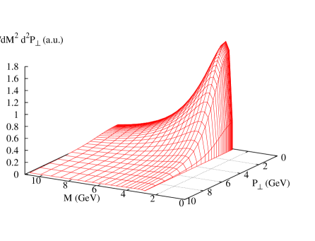
Figure 3: Pair cross-section (in arbitrary units) in the MV model, as a function of ${\boldsymbol{P}}_{\perp}$ and $M$.

In fig. 3, for illustration, we plot the cross-section for the quark pair production as a function of ${\boldsymbol{P}}_{\perp}$ and $M$. We have chosen here a quark mass of $m$=1.5 GeV and the saturation scale  to be $Q_{s}^{2}$=2 GeV². Unsurprisingly, it is peaked at small values of ${\boldsymbol{P}}_{\perp}$ and just above the threshold in the invariant mass $M$ of the pairs.

Examining the behavior of the differential pair cross-section at large $M$ and fixed $P_{\perp}$, or conversely at large $P_{\perp}$ and fixed $M$, we obtain the asymptotic forms,

$$\frac{dN}{dM^{2}d^{2}{\boldsymbol{P}}_{\perp}dY}\mathrel{\mathop{\kern 0.0pt\sim}\limits_{{M\to\infty}\atop{P_{\perp}={\rm const}}}}\frac{\ln^{2}(M^{2})}{M^{4}}\;,$$

$$\frac{dN}{dM^{2}d^{2}{\boldsymbol{P}}_{\perp}dY}\mathrel{\mathop{\kern 0.0pt\sim}\limits_{{P_{\perp}\to\infty}\atop{M={\rm const}}}}\frac{\ln(P_{\perp}^{2})}{P_{\perp}^{4}}\;.$$ (33)

The $1/P_{\perp}^{4}$ and the $1/M^{4}$ behavior, in the stated limits is as one would expect in perturbative QCD (pQCD). Further, the logarithmic prefactors can be related to the collinear logarithms of pQCD which, at leading log order and beyond, are absorbed in the hadronic structure functions.

The occurrence of these logarithms in the CGC framework and their relation to the collinear logs of pQCD can be understood as follows. The CGC formulas obtained in [24] and [1] correspond to color sources from the proton and the nucleus that radiate gluons which fuse into a quark-antiquark pair.

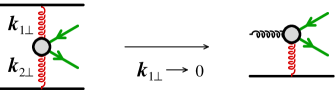
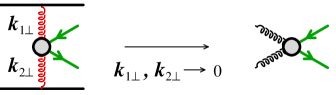
Figure 4: Diagrams in the framework of collinear factorization obtained when one (top), or both (bottom), of the transverse momentum transfer to the produced pair from the proton and nucleus becomes small.

In the limit where both the gluons from the proton and from the nucleus have a small transverse momentum, the CGC formulas reduce to the process $gg\to Q\overline{Q}$ (at leading order) in the collinear factorization framework. Moreover, the integration over the transverse momenta of these gluons produce logarithms that can be interpreted as the first power of the collinear logarithms resummed by the DGLAP equation. Because the large $M$ limit is accessible at leading order in collinear factorization, it is natural to expect two powers of $\ln(M^{2})$ in our formulas corresponding to the limit $|{\boldsymbol{k}}_{1\perp}|$, $|{\boldsymbol{k}}_{2\perp}|\rightarrow 0$. This is shown in the lower diagram of fig. 4. In contrast, the limit of large $P_{\perp}$ of the pair can only be studied at next-to-leading order in the collinear factorization framework. In our formula, as shown in the upper diagram of fig. 4, this corresponds to the limit where only one of the two gluons has a small transverse momentum ($|{\boldsymbol{k}}_{1\perp}|\rightarrow 0$). Hence the single power of $\ln(P_{\perp})$. The relation of higher orders in the collinear factorization framework for pair production to the $k_{\perp}$ factorization framework was explored previously in refs. [26, 96].

4.1.2 Breaking of $k_{\perp}$-factorization

Another important issue, previously studied for the production of single quarks in [30], is that of $k_{\perp}$-factorization. This is illustrated in figure 5, where we display the cross-section versus $P_{\perp}$ for fixed $M$ (left) and versus $M$ for fixed $P_{\perp}$ (right). In these figures, we compare the exact values from eq. (17) (using eq. (6) and eq. (10) to the same expression in the $k_{\perp}$-factorized approximation for pair production.

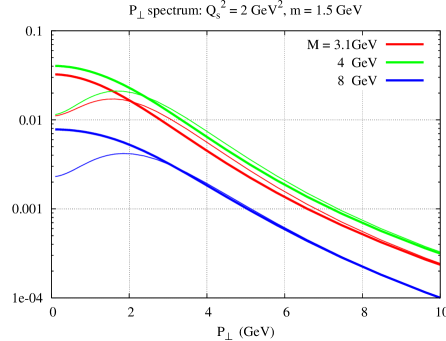
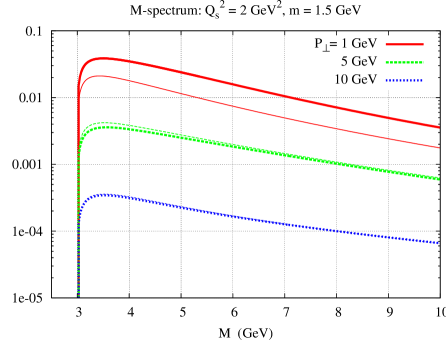
Figure 5: Pair cross-section as a function of ${\boldsymbol{P}}_{\perp}$ for fixed $M$ (left). Pair cross-section as a function of $M$ for fixed ${\boldsymbol{P}}_{\perp}$ (right). The results in the ${\boldsymbol{k}}_{\perp}$-factorized approximation are shown with thin lines.

The $k_{\perp}$-factorized result is obtained by replacing $\phi_{{}_{A}}^{g,q\bar{q}}$ and $\phi_{{}_{A}}^{q\bar{q},q\bar{q}}$ in eq. (6) by

$$\phi_{{}_{A}}^{g,q\bar{q}}({\boldsymbol{k}}_{2\perp};{\boldsymbol{k}}_{\perp})_{\rm fact}\equiv\phi_{{}_{A}}^{g,g}(k_{2\perp})(2\pi)^{2}\left[\delta({\boldsymbol{k}}_{\perp})\!+\!\delta({\boldsymbol{k}}_{\perp}\!-\!{\boldsymbol{k}}_{2\perp})\right]$$

$$\phi_{{}_{A}}^{q\bar{q},q\bar{q}}({\boldsymbol{k}}_{2\perp};{\boldsymbol{k}}_{\perp},{\boldsymbol{k}}_{\perp}^{\prime})_{\rm fact}\equiv\phi_{{}_{A}}^{g,g}(k_{2\perp})$$

$$\qquad\qquad\times(2\pi)^{4}\Big{[}\frac{C_{{}_{F}}}{N}\left(\delta({\boldsymbol{k}}_{\perp}-{\boldsymbol{k}}_{2\perp})\delta({\boldsymbol{k}}_{\perp}^{\prime}-{\boldsymbol{k}}_{2\perp})+\delta({\boldsymbol{k}}_{\perp})\delta({\boldsymbol{k}}_{\perp}^{\prime})\right)$$

$$\qquad\qquad\qquad+\frac{1}{2N^{2}}\left(\delta({\boldsymbol{k}}_{\perp}-{\boldsymbol{k}}_{2\perp})\delta({\boldsymbol{k}}_{\perp}^{\prime})+\delta({\boldsymbol{k}}_{\perp})\delta({\boldsymbol{k}}_{\perp}^{\prime}-{\boldsymbol{k}}_{2\perp})\right)\Big{]}\;.$$

In other words, the limit of $k_{\perp}$-factorization is obtained from “nuclear distributions” very similar to the leading twist formulas in eqs. (15), except that the leading twist 2-point function is replaced by the “all twist” 2-point function. This means that some of the rescattering corrections, but not all of them, can be included in the approximation of $k_{\perp}$-factorization.

The dependence of the ratio of the exact result to the $k_{\perp}$-factorized result, as a function of ${\boldsymbol{P}}_{\perp}$ and $M$, is nicely seen in the 3d plot of fig. 6.

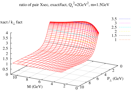
Figure 6: Ratio of the pair cross-section of the full result to the $k_{\perp}$-factorization result as a function of ${\boldsymbol{P}}_{\perp}$ and $M$.

At any fixed $M$, for large $P_{\perp}$, the exact cross-section and the $k_{\perp}$-factorized approximation become identical. (See also the left plot of figure 5.) This is because, in this limit, the quark and the anti-quark become collinear with each of them having a very large transverse momentum. The quark-antiquark pair then scatters off the medium as a gluon would; as in the latter case, this leads to $k_{\perp}$ factorization.

On the contrary, we observe in the right plot of figure 5 (fixed $P_{\perp}$ and large $M$), the exact cross-section and the $k_{\perp}$-factorized approximation are not identical if the fixed value of the transverse momentum of the pair, $P_{\perp}$, is of the order of $Q_{s}$ or smaller. This is because any pair configuration with a small total $P_{\perp}$ is very sensitive to rescatterings; even a small number of additional rescatterings, regardless of the pair invariant mass, may significantly change the transverse momentum of the pair.

Turning now to fixed invariant mass and smaller transverse momentum $P_{\perp}\lesssim Q_{s}$, we note (see left panel of fig. 5) a qualitative change in the behavior of the cross-section due to multiple scattering, high parton density effects. In the $k_{\perp}$-factorized approximation, the pair cross-section shows a bump at ${\boldsymbol{P}}_{\perp}\sim Q_{s}$. Further it is suppressed relative to the exact result for ${\boldsymbol{P}}_{\perp}\leq Q_{s}$. This suppression occurs because $k_{\perp}$-factorization requires that only the quark or the anti-quark – and not both – scatters off the nucleus. The typical transverse momentum taken from the (dilute) proton is rather small; the transverse momentum of the pair is therefore approximately equal to the transverse momentum exchanged during these scatterings on the nucleus–of order $Q_{s}$. Thus, in the $k_{\perp}$-factorized approximation, the pair is less likely to have a total momentum ${\boldsymbol{P}}_{\perp}$ smaller than $Q_{s}$. In contrast, in the exact expression within the MV model, both the quark and the anti-quark get multiply scattered in the target nucleus. Therefore their net momentum can still be smaller than $Q_{s}$. This explains the absence of a bump structure in the exact expression for the ${\boldsymbol{P}}_{\perp}$ distribution of the quark–anti-quark pair. The size of the factorization breaking in this low $P_{\perp}$ region can be as large as a factor 3.

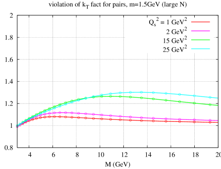
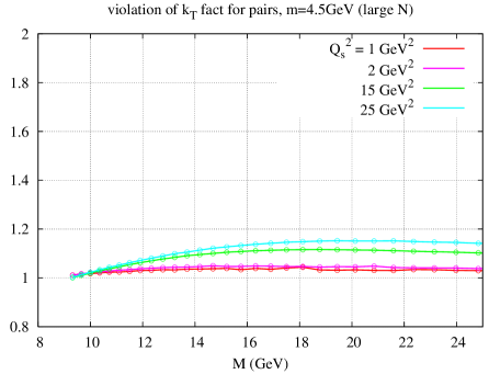
Figure 7: Ratio of the pair yields $dN/dYdM^{2}$ from the exact formula and from the $k_{\perp}$-factorized approximation as a function of $M$ for $m$=1.5 GeV (left) and 4.5 GeV (right).

When we integrate the cross-section over the total momentum ${\boldsymbol{P}}_{\perp}$, the magnitude of the factorization breaking, shown in fig. 7, is about $10\%$ for $m$=1.5 GeV and $Q_{s}^{2}$= 2 GeV². The latter is a typical value associated with central RHIC collisions. For the larger values of $Q_{s}$ that may be accessed in forward Deuteron-Gold collisions at RHIC and the LHC, the magnitude of the breaking is maximally $30\%$. Note that even for large invariant masses, the ratio returns to unity very slowly. This again is due to the fact that in the low ${\boldsymbol{P}}_{\perp}$ region, which contributes significantly to the integrated cross-section, the relative magnitude of violation of $k_{\perp}$-factorization is constant for large $M$. As for the case of single quark production [30], fig. 7 shows that the breaking of $k_{\perp}$-factorization grows with increasing $Q_{s}$ while it is systematically weaker for larger quark masses.

Finally, we observe in fig. 7 that, precisely at the pair threshold, the ratio of the exact to the $k_{\perp}$-factorized expression is unity. As is clear from the left panel of fig. 6, this ratio is not unity for any specific $P_{\perp}$ but is a property of the distribution integrated over $P_{\perp}$. This observation seems related to the following fact: at threshold, the quark and the antiquark are at rest in the rest frame of the pair. When boosted to the lab frame, they have the same momenta at threshold and are therefore collinear. A pair made of a collinear quark and antiquark is very similar to an octet gluon. The correlator of two Wilson lines satisfies a sum rule which ensures that the momentum integrated distributions are unchanged even if the momenta are redistributed by re-scattering. It is therefore plausible that the integrated pair distribution at threshold, in analogy to the gluon distribution, is insensitive to re-scatterings.

4.1.3 Nuclear size ($Q_{s}^{2}$) dependence

In the MV model, the nuclear size dependence arises only through the radius $R$ and the saturation scale $Q_{s}^{2}$. In the MV model, the saturation scale $Q_{s}^{2}$ is independent of the energy and also depends on the atomic mass number roughly as $A^{1/3}$. Alternately, the scale $\mu_{{}_{A}}^{2}$ is used, which determines the number of color charges in the nucleus, per unit of transverse area. It is proportional to $A^{1/3}$. The relation between the two scales is specified in footnote  15.

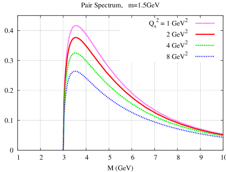
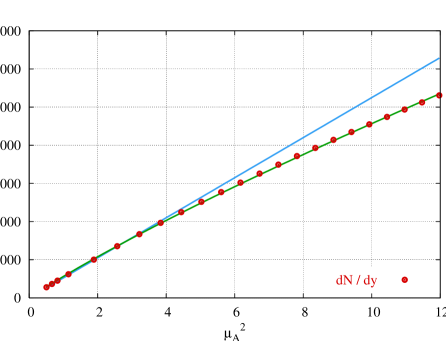
Figure 8: Left: invariant mass spectrum of $Q\overline{Q}$ pairs for different values of the saturation scale. Right: integrated quark yield as a function of $\mu_{{}_{A}}^{2}\sim A^{1/3}$, the scale specifying the number of color charges per unit transverse area. Points: numerical evaluation of the cross-section. Solid line: fit by a function in $\mu_{{}_{A}}^{2}/\ln(\mu_{{}_{A}}^{2})$.

We first examine the integrated quark yield per unit rapidity (at fixed impact parameter) as a function of the nuclear size. This quantity is displayed in figure 8, in differential form as a function of $M$ on the left plot and integrated as a function of $\mu_{{}_{A}}^{2}\propto A^{1/3}$ on the right plot. Because one naively expects, for heavy quarks, a scaling with the number of binary collisions, namely $A^{1/3}$, the curves in the left plot have been divided by a factor $\mu_{{}_{A}}^{2}$. The residual dependence on the saturation scale is therefore a departure from the binary scaling hypothesis. As one can see, when the saturation scale increases, the differential yield decreases, albeit in a very moderate fashion (note that the vertical axis for the left plot is a linear axis). When we integrate these functions over the invariant mass in order to obtain the total quark yield, we see that it is very close to a linear function of $\mu_{{}_{A}}^{2}$, confirming the fact that the departure from binary scaling is small. This departure is a small reduction of the yield compared to binary scaling, and one can fit the dependence of $dN/dY$ on $\mu_{{}_{A}}^{2}$ by a function that behaves like $\mu_{{}_{A}}^{2}/\ln(\mu_{{}_{A}}^{2})$.

Another quantity, whose dependence on the nuclear size is of phenomenological interest, is the nuclear modification factor $R_{pA}$. It is defined as the ratio between the yield in $pA$ collisions to the yield in $pp$ collisions, normalized by the number of binary collisions,

$$R_{pA}\equiv\frac{1}{A^{1/3}}\;\frac{\left.\frac{dN}{dM^{2}d^{2}{\boldsymbol{P}}_{\perp}dY}\right|_{pA}}{\left.\frac{dN}{dM^{2}d^{2}{\boldsymbol{P}}_{\perp}dY}\right|_{pp}}\;.$$ (35)

Indeed, this nuclear modification factor for $pA$ collisions is essential for establishing a baseline for “normal nuclear suppression” when looking for potential quark gluon plasma suppression effects on the yield of $J/\psi$’s in nucleus-nucleus collisions.

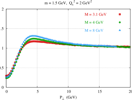
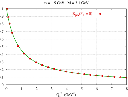
Figure 9: Left: nuclear modification factor for the production of $Q\overline{Q}$ pairs, as a function of their transverse momentum. Right: dependence of the modification factor at low $P_{\perp}$ as a function of $Q_{s}$. The solid line is fit by a function that behaves as $1/Q_{s}^{2}$.

In the left plot of figure 9, we display this ratio as a function of $P_{\perp}$, for a given $Q_{s}$ and various fixed invariant masses. One can see here a behavior which is very similar to what was previously observed for gluon production in $pA$ collisions (see [15] for instance): there is a suppression at low $P_{\perp}$ and an enhancement at high $P_{\perp}$, relative to perfect scaling with the number of binary collisions.

The plot on the right of figure 9 shows how the value of the suppression at small momentum changes with varying saturation scale. We show this for an invariant mass just above the pair production threshold because this is the dominant kinematical domain contributing to the production of bound states (such as the $J/\psi$). We observe that the pair yield, for large $Q_{s}^{2}$, behaves as $1/Q_{s}^{2}$. Up to a logarithm (due to the small difference between $Q_{s}^{2}$ and $\mu_{{}_{A}}^{2}$), this corresponds to a scaling like $1/L$ where $L$ is the longitudinal size of the nucleus. This $1/L$ dependence is well known from the super-penetration [97, 98] of electron-positron pairs through metallic foils (often called the “Chudakov effect”) and was noted previously in the QCD case [99, 100, 55, 56], by looking at the propagation of $Q\overline{Q}$ states through a random distribution of color fields. This result is in contrast to the Glauber like form $\exp(-C\rho\sigma L)$ that is often assumed, where $\sigma$ is the inelastic $J/\psi$-nucleon cross-section, $\rho$ is the nuclear density, and $C$ is constant number. Such an exponential form assumes successive independent collisions, and the decreasing exponential is thus the probability that the $J/\psi$ has survived after propagating through a length $L$ of nuclear matter. However, for the values of $Q_{s}$ probed at present energies it may be difficult to distinguish between the linear and exponential forms.

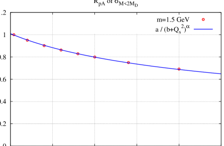
Figure 10: Ratio of the pair cross-sections with the invariant mass $M<2M_{D}$ for “pp” and “pA.” On the basis of the Color Evaporation Model, this is interpreted as the normal nuclear suppression factor of the charmonium. The parameters of the fitting curve are $a=1.51(6)~{}\mbox{GeV}^{2}$, $b=2.65(16)~{}\mbox{GeV}^{2}$ and $\alpha=0.417(15)$.

To observe how this pattern of suppression for producing $Q\overline{Q}$ pairs translates into the nuclear $J/\psi$ suppression, we will consider the phenomenological “Color Evaporation” model (CEM). This model assumes that the yield of $J/\psi$’s is obtained by integrating the yield of $Q\overline{Q}$ pairs over the invariant mass of the pairs, from production threshold of a charm quark pair to the threshold for the production of a pair of $D$ mesons, up to an overall constant prefactor. This can be expressed as

$$\frac{dN_{J/\psi}}{dYd^{2}{\boldsymbol{P}}_{\perp}}\mathrel{\mathop{\kern 0.0pt=}\limits_{CEM}}F_{J/\psi}\int_{4m^{2}}^{4m_{{}_{D}}^{2}}dM^{2}\;\frac{dN}{dYd^{2}{\boldsymbol{P}}_{\perp}dM^{2}}\;.$$ (36)

If hadronization takes place outside of the nucleus (a legitimate assumption for $J/\psi$ production at high energy), one can assume that the prefactor $F_{J/\psi}$ is the same for $pA$ and $pp$ collisions. It therefore cancels out in the ratio $R_{pA}$. In figure 10, we represent the ratio $R_{pA}$ for $J/\psi$ production in the CEM , as a function of the saturation momentum $Q_{s}$. The solid line represents a fit of this ratio by a power of $Q_{s}$. One sees that the nuclear modification ratio is well reproduced by a power law, $Q_{s}^{-0.8}$, namely $A^{-0.13}$ or $1/L^{0.4}$. We get a smaller power of $Q_{s}$ relative to figure 9 simply because we here integrate over $P_{\perp}$. The greater suppression at $P_{\perp}=0$ is attenuated by the enhancement present at higher $P_{\perp}$’s. This pattern of $J/\psi$ suppression is not very sensitive to the precise mass of the $c$ quark.

4.1.4 Dependence on the quark mass

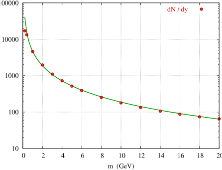
Figure 11: Dots: pair yield as a function of the mass of the quarks. Solid line: fit by a function that behaves like $\ln(m)/m^{2}$.

Finally, we shall discuss in the MV model, the dependence of the total $Q\overline{Q}$ yield as a function of the mass of the quarks. This is plotted in figure 11 (per unit rapidity; as emphasized, there is no $Y$ dependence in the MV model). One finds that, for quarks masses larger than the saturation scale, the yield behaves as $\ln(m)/m^{2}$, in agreement with what one expects from perturbation theory. The leading $1/m^{2}$ simply comes from integrating the $1/P_{\perp}^{4}$ behavior from $p_{\perp}\sim m$ to $\infty$. The additional factor of $\ln(m)$ arises from the intermediate $P_{\perp}$ region, $Q_{s}\lesssim P_{\perp}\lesssim m$ where there is a deviation from the $1/P_{\perp}^{4}$ behavior for masses below the saturation scale. The yield therefore flattens out and does not grow as fast as $1/m^{2}$ anymore. This implies that the limit of zero quark mass is less singular than it is at leading twist. In the latter case, the yield would keep growing as $1/m^{2}$ all the way up into to the infrared region.

4.2 Multiple scattering a la MV + quantum evolution a la BK

4.2.1 Kinematics for small $x$ evolution and initial conditions

Our previous results, in the MV model, only included multiple scattering effects on quark pair production in proton-nucleus collisions. Quantum evolution effects due to gluon bremsstrahlung are not included. At high energies, gluons with a very small longitudinal momentum fraction $x$ may be probed in the projectiles. It therefore becomes necessary to resum powers of $\alpha_{s}\ln(x_{0}/x)$. These corrections cause leading twist shadowing of gluon distributions. Because the initial condition for small $x$ quantum evolution is not the same in protons and nuclei, quantum evolution is yet another effect – in addition to the multiple scatterings already included in the MV model – that makes the cross-sections in $pp$ and $pA$ collisions differ.

As discussed in section 3, we will study these quantum evolution effects in the framework of the Balitsky-Kovchegov (BK) equation. We noted there that the nuclear saturation scale, obtained from solutions of the BK equation, now depends on both $A$ and the rapidity of the gluons probed in the nucleus. The former dependence comes from the initial condition, which is taken to be the McLerran-Venugopalan model, while the energy dependence follows from solutions of the BK equation. With the approximations for the correlators obtained by substituting the BK result for the l.h.s. of eq. (31) in eqs. (LABEL:eq:largeN-25), we are in a position to study how our previous multiple scattering results are modified by small $x$ quantum evolution.

In our kinematics, the $+$ component of the gluon that comes from the proton is related to the $+$ momentum of the pair by the relation

$$k_{1}^{+}=p^{+}+q^{+}\;,$$ (37)

and similarly the $-$ momentum taken from the nucleus is given by the relation

$$k_{2}^{-}=p^{-}+q^{-}\;.$$ (38)

The longitudinal momentum fractions of the gluons probed in the proton and in the nucleus – respectively $x_{p}$ and $x_{{}_{A}}$ – are related to the $+$ component of the momentum of the proton and to the $-$ component of the momentum of a nucleon in the nucleus by :

$$x_{p}=\frac{k_{1}^{+}}{P_{p}^{+}}\quad,\qquad x_{{}_{A}}=\frac{k_{2}^{-}}{P_{{}_{A}}^{-}}\;.$$ (39)

Using $P_{p}^{+}=P_{{}_{A}}^{-}=\sqrt{s/2}$, we can express these momentum fractions in terms of the transverse momentum of the quark and the antiquark and their rapidities (see the discussion following eq. (16)) as

$$x_{p,_{A}}=\frac{{\omega_{p}\,e^{\pm y_{p}}+\omega_{q}\,e^{\pm y_{q}}}}{\sqrt{s}}\;,$$ (40)

where $\omega_{p}^{2}\equiv{\boldsymbol{p}}_{\perp}^{2}+m^{2}$ and $\omega_{q}^{2}\equiv{\boldsymbol{q}}_{\perp}^{2}+m^{2}$. Alternatively, we can also express the momentum fractions in terms of the kinematical parameters of the pair, $P_{\perp},M,Y$ as

$$x_{p,_{A}}=\sqrt{\frac{P_{\perp}^{2}+M^{2}}{s}}\;e^{\pm Y}\;.$$ (41)

This latter form of $x_{p,A}$ makes obvious the fact that when we integrate over $\tilde{q}$ and $\phi$ in eq. (17), the values of $x_{p}$ and $x_{{}_{A}}$ remain constant. This is very similar to gluon production, where the values of $x_{p,_{A}}$ are also fully determined by the final state.

Our approach has an important caveat that we should discuss before presenting the results. We have argued elsewhere that the MV model, used here as the initial condition when solving the BK equation, is a good description of a nucleus at moderate value of $x$. This value is often estimated  to be of order of $x_{0}=10^{-2}$. By solving the BK equation, one obtains the value of the gluon distributions at any value of $x$ smaller than this $x_{0}$. However, in the calculation of the $Q\overline{Q}$ cross-section, depending on the kinematics of the final state, we may need the unintegrated gluon distributions for values of $x_{p}$ or $x_{{}_{A}}$ (or both) that are larger than $x_{0}$. From eq. (41), we observe that this will happen in one of the projectiles if $|Y|$ becomes large, or in both of them at moderate $Y$ and large $P_{t}$ or $M$. Therefore, the MV initial condition at $x=x_{0}$ supplemented by BK evolution, is not sufficient to cover the entire kinematical range. One possibility would be to simply dismiss the points $P_{t},Y,M$, where this problem occurs, on the grounds that these points are “contaminated” by large-$x$ physics. Ideally, one should try to constrain the necessary gluon distributions at large $x$ from existing data. However, for the purposes of the qualitative discussion presented here, we follow an intermediate path: we make a simple ansatz for the gluon distributions that continues the MV initial condition at $x\geq x_{0}$.

Because the numerical evaluation of the pair cross-section is done with eq. (27), we need only to make such an ansatz for the proton unintegrated gluon distribution $\varphi_{p}$ and for the 3-point function $\phi_{{}_{A}}^{g,q\bar{q}}({\boldsymbol{k}}_{2\perp};{\boldsymbol{k}}_{\perp}|x)$ in the nucleus. One generally requires, from quark counting rules, that for values of $x$ close to unity, all gluon distributions vanish as $(1-x)^{4}$. We adopt here a simple ansatz that implements this behavior;

$$\mbox{for\ \ }x\geq x_{0}\;,\qquad\phi_{{}_{A}}^{g,q\bar{q}}({\boldsymbol{k}}_{2\perp};{\boldsymbol{k}}_{\perp}|x)\equiv\left(\frac{1-x}{1-x_{0}}\right)^{4}\;\phi_{{}_{A}}^{g,q\bar{q}}({\boldsymbol{k}}_{2\perp};{\boldsymbol{k}}_{\perp}|x_{0})\;,$$ (42)

where the denominator $(1-x_{0})^{4}$ ensures the continuity of $\phi_{{}_{A}}^{g,q\bar{q}}({\boldsymbol{k}}_{2\perp};{\boldsymbol{k}}_{\perp}|x)$ at $x=x_{0}$. We make the same ansatz for $\varphi_{p}$. Because the details of how these gluon distributions vanish when $x\to 1$ are somewhat arbitrary, readers should note that results for the cross-section in kinematic regions dominated by large values of $x$ (in one or both of the projectiles) contain a large systematic uncertainty.

This uncertainty is reduced when the center of mass energy $\sqrt{s}$ of the collision increases because the values of $x_{p,_{A}}$ decrease and the corresponding physics is less sensitive to the initial conditions. To ensure a significant region in the kinematical parameters $P_{\perp},Y,M$ of the pair where the cross-section is not affected by this arbitrariness, all numerical calculations presented in the following subsections have been performed for the center of mass energy of the LHC, $\sqrt{s}=8.5~{}$TeV. At RHIC energies, if $x_{0}=10^{-2}$, there is no region in phase-space which is not contaminated by the large $x$ behavior of one (or both) of the projectiles. Therefore, a realistic description of RHIC results in this framework would require a less simplistic ansatz than eq. (42). Alternately, it may very well be the case that MV initial conditions may be applicable in large nuclei at larger values of $x_{0}$. A systematic study is required but is beyond the scope of this paper.

4.2.2 Rapidity dependence

We shall now use the solution of the BK equation with the extrapolation done in eq. (42), to compute the rapidity dependence of the pair cross-section in eq. (17). In fig. 12, we show the rapidity distribution of $c{\bar{c}}$ pairs, for a fixed value of the invariant mass $M=3.1$ GeV, and several values of the transverse momentum of the pair. The fact that the first derivative in $x$ of the unintegrated gluon distributions is not preserved by the ansatz  of eq. (42) shows up in the cross-section as a discontinuity in the slope in $Y$ of $dN/dYdM^{2}d^{2}{\boldsymbol{P}}_{\perp}$. On the plots, we have indicated the region in $Y$ affected by this extrapolation by plotting only a solid line in these regions (their boundaries can be easily determined from eq. (41)). The central region in rapidity - unaffected by this extrapolation - shrinks as one increases the transverse momentum of the pair, or its invariant mass.

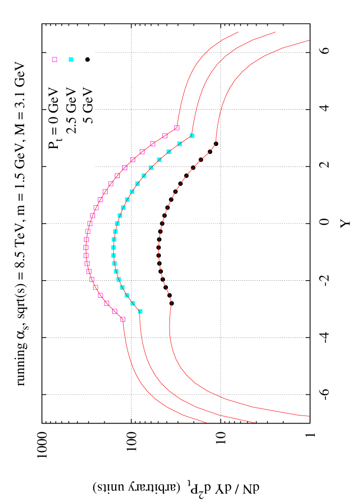
Figure 12: The rapidity distribution of quark–anti-quark pairs in pA collisions, for an invariant mass $M=3.1~{}$GeV and various values of the transverse momentum $P_{\perp}$. The dots indicate the region in $Y$ which is not sensitive to the extrapolation done at large $x$. (See eq. (42)).

4.2.3 Cronin effect and shadowing

To study deviations from the scaling with the number of binary collisions, one can compute the ratio $R_{pA}$ defined in eq. (35). In figure 13, we display this ratio as a function of $P_{\perp}$ for different values of the rapidity (again the invariant mass is set to $M=3.1$ GeV). On the left, the cross-section has been computed with the solution of the BK equation with fixed coupling, while on the right the BK equation was solved with a running coupling. There are small quantitative differences between fixed and running coupling, but the overall qualitative behavior of $R_{pA}$ is unaffected.

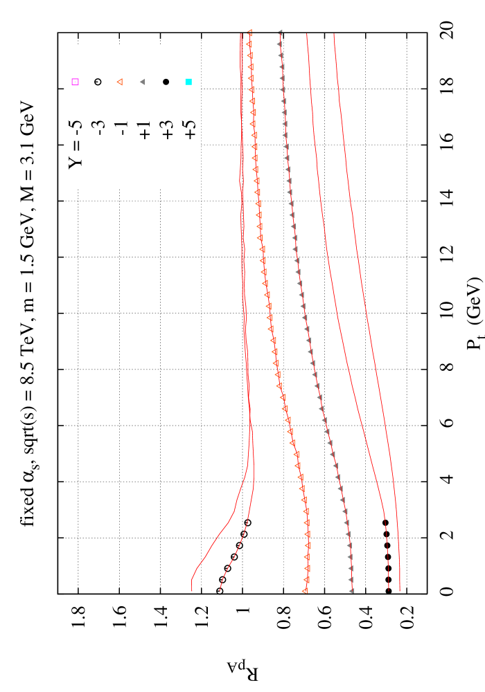
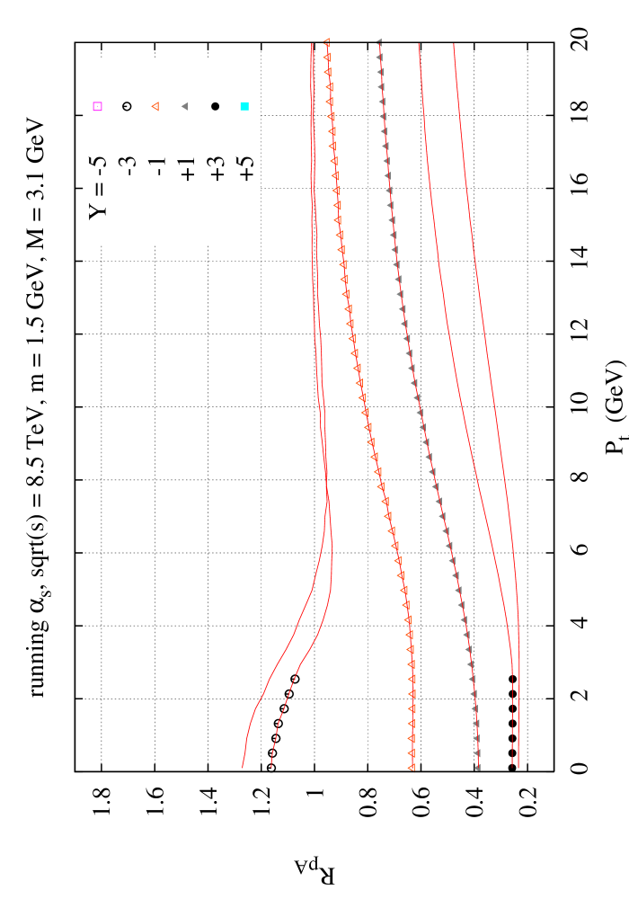
Figure 13: Nuclear modification factor for $Q\overline{Q}$ pairs at LHC center of mass energy, as a function of the transverse momentum of the pair. The pair invariant mass is just above the charm pair threshold ($M=3.1$ GeV) and the rapidity is varied from $-5$ to $+5$. Left: the $x$ dependence is obtained from the BK equation with fixed coupling ($\alpha_{s}N_{c}/\pi=0.2$). Right: the $x$ dependence is obtained from the BK equation with running coupling. Regions on the plot represented by only a solid line and no dots are sensitive to the large-$x$ extrapolation done in eq. (42).

As one can see, the only region for which the ratio $R_{pA}$ goes over 1 is at the most negative rapidities. As the rapidity increases above $Y=-3$, $R_{pA}$ decreases significantly, and remains below 1 at all $P_{\perp}$’s.

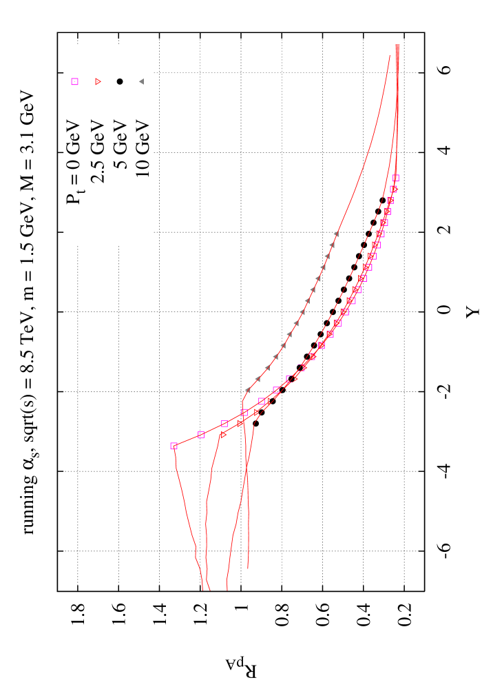
Figure 14: The rapidity dependence of the nuclear modification ration, at fixed $M$ and for several values of $P_{\perp}$. The regions affected by the large $x$ extrapolation are indicated by the absence of dots.

An alternative way to view the same information is to display $R_{pA}$ as a function of the rapidity $Y$, for fixed values of $P_{\perp}$, as in figure 14. (Note that for a limited region in $Y$, and for fixed $P_{\perp}$, it is proportional to the widely used variable $x_{F}$.) On this plot, one sees a rapid decrease of $R_{pA}$ with $Y$. In our computation, this drop seems to start around $Y=-3$. Keep in mind however that the lower rapidity region is plagued by artifacts introduced by the large-$x$ extrapolation–the drop may in fact start earlier. Moreover, one sees on this plot that the decrease of $R_{pA}$ with $Y$ is very rapid at negative $Y$, and slows down at positive rapidities. This is reminiscent of the very fast disappearance of the Cronin peak in the study of $R_{pA}$ for gluons via the BK equation [42, 20]. One also observes that the pattern of this suppression is almost independent of $P_{\perp}$ at small $P_{\perp}$, and that the $P_{\perp}$ dependence becomes manifest only above $P_{\perp}\sim 5~{}$GeV. These results are qualitatively similar to those observed for the rapidity dependence of the nuclear modification factor at lower energies.

5 Conclusions

In this paper, we have explored the formalism developed in ref. [1] for pair production in proton nucleus collisions. We presented explicit results for two models, each of which corresponds to a particular limit of high parton densities realized in the Color Glass Condensate formalism of high energy QCD. In the first case, the McLerran-Venugopalan model, multiple scattering effects on pair production were studied in the absence of shadowing effects. We obtained results in this model for the pair cross-sections as a function of the invariant mass, the transverse momenta of the pairs, as well as their dependence on nuclear size and the quark mass. For large transverse momenta or invariant masses, both the power law dependence on these scales, and the accompanying logarithms can be interpreted in terms of the leading kinematic behavior in the collinear factorization framework of perturbative QCD. We also studied, in the MV model, the extent of the violation of $k_{\perp}$ factorization.

We next considered a model, where both multiple scattering and small $x$ quantum evolution (shadowing) effects are included. In the limit of large $N_{c}$ and large $A$, the energy evolution of the multi-parton correlators in pair cross-sections can be described in terms of the Balitsky-Kovchegov equation. We solved the BK equation numerically, for both fixed and running coupling, in order to determine the rapidity distribution of pairs as well as the evolution of the nuclear modification factor $R_{pA}$ as a function of rapidity. As in the gluon case, for fixed $P_{\perp}$, one notes a rapid initial depletion of $R_{pA}$ with rapidity followed by a much slower depletion at larger rapidities. We emphasize that at RHIC energies our results may be sensitive to particular ansätze for unintegrated gluon distributions at large $x$; at LHC energies, this sensitivity is considerably weaker.

The studies in this paper provide insight into the systematics of pair production and the dependence of the results on the quark masses, the system size and the center of mass energy. Detailed phenomenological studies of $J/\psi$ and open charm production are underway and will be reported on in a followup to this work [75].

While this manuscript was being prepared for publication, ref. [102] appeared. The authors of ref. [102] correctly argue that the results of ref. [1] can be extended to include small $x$ quantum evolution effects. This is precisely what is done here; quantum evolution effects are included by solving the BK equation for the unintegrated gluon distributions in eq. 10. Quantitative results from the solution of the BK equation for the evolution of pair cross-sections with energy/rapidity are presented in section 4.2.

References

- [1] J.P. Blaizot, F. Gelis, R. Venugopalan, Nucl. Phys. A 743, 57 (2004).
- [2] L.V. Gribov, E.M. Levin, M.G. Ryskin, Phys. Rept. 100, 1 (1983).
- [3] A.H. Mueller, J-W. Qiu, Nucl. Phys. B 268, 427 (1986).
- [4] J.P. Blaizot, A.H. Mueller, Nucl. Phys. B 289, 847 (1987).
- [5] L.D. McLerran, R. Venugopalan, Phys. Rev. D 49, 2233 (1994).
- [6] L.D. McLerran, R. Venugopalan, Phys. Rev. D 49, 3352 (1994).
- [7] L.D. McLerran, R. Venugopalan, Phys. Rev. D 50, 2225 (1994).
- [8] E. Iancu, A. Leonidov, L.D. McLerran, Nucl. Phys. A 692, 583 (2001).
- [9] E. Iancu, A. Leonidov, L.D. McLerran, Phys. Lett. B 510, 133 (2001).
- [10] E. Ferreiro, E. Iancu, A. Leonidov, L.D. McLerran, Nucl. Phys. A 703, 489 (2002).
- [11] E. Iancu, A. Leonidov, L.D. McLerran, Lectures given at Cargese Summer School on QCD Perspectives on Hot and Dense Matter, Cargese, France, 6-18 Aug 2001, hep-ph/0202270.
- [12] E. Iancu, R. Venugopalan, Quark Gluon Plasma 3, Eds. R.C. Hwa and X.N.Wang, World Scientific, hep-ph/0303204.
- [13] A.H. Mueller, Lectures given at the International Summer School on Particle Production Spanning MeV and TeV Energies (Nijmegen 99), Nijmegen, Netherlands, 8-20, Aug 1999, hep-ph/9911289.
- [14] J. Jalilian-Marian, Y. Kovchegov, Prog. Part. Nucl. Phys. 56, 104 (2006).
- [15] J.P. Blaizot, F. Gelis, R. Venugopalan, Nucl. Phys. A 743, 13 (2004).
- [16] Yu.V. Kovchegov, A.H. Mueller, Nucl. Phys. B 529, 451 (1998).
- [17] M.A. Braun, Phys. Lett. B 483, 105 (2000).
- [18] M.A. Braun, Eur. Phys. J. C 20, 517 (2001).
- [19] B.Z. Kopeliovich, J. Raufeisen, hep-ph/0305094.
- [20] D. Kharzeev, Yu. Kovchegov, K. Tuchin, Phys. Rev. D 68, 094013 (2003).
- [21] I. Balitsky, Phys. Rev. D 70, 114030 (2004).
- [22] A. Krasnitz, Y. Nara, R. Venugopalan, Nucl. Phys. A 727, 427 (2003).
- [23] A. Krasnitz, Y. Nara, R. Venugopalan, Phys. Rev. Lett. 87, 192302 (2001).
- [24] F. Gelis, R. Venugopalan, Phys. Rev. D 69, 014019 (2004).
- [25] J.C. Collins, R.K. Ellis, Nucl. Phys. B 360, 3 (1991).
- [26] S. Catani, M. Ciafaloni, F. Hautmann, Nucl. Phys. B 366, 135 (1991).
- [27] P. Hagler, R. Kirschner, A. Schafer, L. Szymanowski, O. Teryaev, Phys. Rev. D 63, 077501 (2001).
- [28] A.V. Lipatov, V.A. Saleev, N.P. Zotov, hep-ph/0112114.
- [29] F. Yuan, K.T. Chao, Phys. Rev. Lett. 87, 022002 (2001).
- [30] H. Fujii, F. Gelis, R. Venugopalan, Phys. Rev. Lett. 95, 162002 (2005).
- [31] J. Jalilian-Marian, A. Kovner, A. Leonidov, H. Weigert, Nucl. Phys. B 504, 415 (1997).
- [32] J. Jalilian-Marian, A. Kovner, A. Leonidov, H. Weigert, Phys. Rev. D 59, 014014 (1999).
- [33] J. Jalilian-Marian, A. Kovner, A. Leonidov, H. Weigert, Phys. Rev. D 59, 034007 (1999).
- [34] J. Jalilian-Marian, A. Kovner, A. Leonidov, H. Weigert, Erratum. Phys. Rev. D 59, 099903 (1999).
- [35] A. Kovner, G. Milhano, Phys. Rev. D 61, 014012 (2000).
- [36] A. Kovner, G. Milhano, H. Weigert, Phys. Rev. D 62, 114005 (2000).
- [37] I. Balitsky, Nucl. Phys. B 463, 99 (1996).
- [38] J. Jalilian-Marian, A. Kovner, L.D. McLerran, H. Weigert, Phys. Rev. D 55, 5414 (1997).
- [39] K. Rummukainen, H. Weigert, hep-ph/0309306.
- [40] Yu.V. Kovchegov, Phys. Rev. D 54, 5463 (1996).
- [41] Yu.V. Kovchegov, Phys. Rev. D 61, 074018 (2000).
- [42] J.L. Albacete, N. Armesto, A. Kovner, C.A. Salgado, U.A. Wiedemann, Phys. Rev. Lett. 92, 082001 (2004).
- [43] M.A. Braun, Eur. Phys. J. C 16, 337 (2000).
- [44] M. Lublinsky, Eur. Phys. J. C 21, 513 (2001).
- [45] E. Levin, M. Lublinsky, Nucl. Phys. A 696, 833 (2001).
- [46] K. Golec-Biernat, L. Motyka, A.M. Stasto, Phys. Rev. D 65, 074037 (2002).
- [47] E. Gotsman, M. Kozlov, E. Levin, U. Maor, E. Naftali, Nucl. Phys. A 742, 55 (2004).
- [48] J.L. Albacete ,N. Armesto, J.G. Milhano, C.A. Salgado, U.A. Wiedemann, Phys. Rev. D 71, 014003 (2005).
- [49] E.M. Levin, K. Tuchin, Nucl. Phys. B 573, 833 (2000).
- [50] D.N. Triantafyllopoulos, Nucl. Phys. B 648, 293 (2003).
- [51] S. Munier, R. Peschanski, Phys. Rev. Lett. 91, 232001 (2003).
- [52] S. Munier, R. Peschanski, Phys. Rev. D 69, 034008 (2004).
- [53] S. Munier, R. Peschanski, Phys. Rev. D 70, 077503 (2004).
- [54] A. Kovner, U. Wiedemann, Phys. Rev. D 64, 114002 (2001).
- [55] H. Fujii, Nucl. Phys. A 709, 236 (2002).
- [56] H. Fujii, T. Matsui, Phys. Lett. B 545, 82 (2002).
- [57] Yu. Dokshitzer, Sov. Phys. JETP 46, 641 (1977).
- [58] G. Altarelli, G. Parisi, Nucl. Phys. B 126, 298 (1977).
- [59] V.N. Gribov, L.N. Lipatov, Sov. J. Nucl. Phys. 15, 438 (1972).
- [60] V.N. Gribov, L.N. Lipatov, Sov. J. Nucl. Phys. 15, 675 (1972).
- [61] A. Dumitru, L.D. McLerran, Nucl. Phys. A 700, 492 (2002).
- [62] A. Dumitru, J. Jalilian-Marian, Phys. Rev. Lett. 89, 022301 (2002).
- [63] F. Gelis, J. Jalilian-Marian, Phys. Rev. D 66, 014021 (2002).
- [64] F. Gelis, J. Jalilian-Marian, Phys. Rev. D 66, 094014, (2002).
- [65] F. Gelis, K. Kajantie, T. Lappi, Phys. Rev. C. 71, 024904 (2005).
- [66] F. Gelis, K. Kajantie, T. Lappi, hep-ph/0508229, to appear in Phys. Rev. Lett.
- [67] S.S. Adler, et al., (PHENIX Collaboration) Phys. Rev. Lett. 96, 012304 (2006).
- [68] J. Adams, et al., (STAR Collaboration) Phys. Rev. Lett. 94, 062301 (2005).
- [69] B. Alessandro, et al., (NA50 Collaboration) Eur. Phys. J. C 39, 335 (2005).
- [70] B. Alessandro, et al., (NA50 Collaboration) Eur. J. Phys. C 33, 31 (2004).
- [71] H.K. Wohri, et al., (NA60 Collaboration) Eur. J. Phys. C 43, 407 (2005).
- [72] D. Kharzeev, K. Tuchin, Nucl. Phys. A 735, 248 (2004).
- [73] D. Kharzeev, K. Tuchin, hep-ph/0510358.
- [74] F.O. Duraes, F.S. Navarra, M. Nielsen, Phys. Rev. C 68, 044904 (2003).
- [75] H. Fujii, F. Gelis, R. Venugopalan, In preparation.
- [76] T. Lappi, Phys. Rev. C 67, 054903 (2003).
- [77] F. Gelis, Y. Methar-Tani, hep-ph/0512079.
- [78] S. Jeon, R. Venugopalan, Phys. Rev. D 70, 105012 (2004).
- [79] S. Jeon, R. Venugopalan, Phys. Rev. D 71, 125003 (2005).
- [80] D. Kharzeev, M. Nardi, Phys. Lett. B 507, 121 (2001).
- [81] D. Kharzeev, E. Levin, M. Nardi, Nucl. Phys. A 730, 448 (2004).
- [82] T. Hirano, Y. Nara, nucl-th/0404039.
- [83] A. Dumitru, J. Jalilian-Marian, Phys. Lett. B 547, 15 (2002).
- [84] F. Gelis, J. Jalilian-Marian, Phys. Rev. D 67, 074019 (2003).
- [85] D. Kharzeev, E. Levin, L.D. McLerran, Phys. Lett. B 561, 93 (2003).
- [86] R. Baier, A. Kovner, U.A. Wiedemann, Phys. Rev. D 68, 054009 (2003).
- [87] J. Jalilian-Marian, Y. Nara, R. Venugopalan, Phys. Lett. B 577, 54 (2003).
- [88] L.D. McLerran, R. Venugopalan, Phys. Rev. D 59, 094002 (1999).
- [89] F. Gelis, A. Peshier, Nucl. Phys. A 697, 879 (2002).
- [90] K. Tuchin, Phys. Lett. B 593, 66 (2004).
- [91] A. Ayala, J. Jalilian-Marian, L.D. McLerran, R. Venugopalan, Phys. Rev. D 52, 2935 (1995).
- [92] A. Ayala, J. Jalilian-Marian, L.D. McLerran, R. Venugopalan, Phys. Rev. D 53, 458 (1996).
- [93] I. Arsene, et al., (BRAHMS collaboration) Phys. Rev. Lett. 93, 242303 (2004).
- [94] K. Golec-Biernat, M. Wüsthoff, Phys. Rev. D 59, 014017 (1999).
- [95] K. Golec-Biernat, M. Wüsthoff, Phys. Rev. D 60, 114023 (1999).
- [96] S. Catani, M. Ciafaloni, F. Hautmann, Phys. Lett. B 242, 97 (1990).
- [97] L.L. Nemenov, Sov. J. Nucl. Phys. 34, 726 (1981).
- [98] V.I. Lyuboshitz, M.I. Podgorestskii, JETP 54, 827 (1981).
- [99] G. Baym, Adv. Nucl. Phys. 22, 101 (1996).
- [100] H. Heiselberg, G. Baym, B. Blaettel, L.L. Frankfurt, M. Strikman, Phys. Rev. Lett. 67, 2946 (1991).
- [101] N. Brambilla, et al., hep-ph/0412158.
- [102] Yu.V. Kovchegov, K. Tuchin, hep-ph/0603055.