Interesting radiative patterns of neutrino mass
in an $\mbox{SU}(3)_{C}\otimes\mbox{SU}(3)_{L}\otimes\mbox{U}(1)_{X}$ model
with right-handed neutrinos

Abstract

We investigate a simple model of neutrino mass based on $\mbox{SU}(3)_{C}\otimes\mbox{SU}(3)_{L}\otimes\mbox{U}(1)_{X}$ gauge unification. The Yukawa coupling of the model has automatic lepton-number symmetry which is broken only by the self-couplings of the Higgs boson. At tree level neutrino spectrum contains three Dirac fermions, one massless and two degenerate in mass. At the two loop-level, neutrinos obtain Majorana masses and correct the tree-level result which naturally gives rise to an inverted hierarchy mass pattern and interesting mixing which can fit the current data with minor fine-tuning. In another scenarios, one can pick the scales such that the loop-induced Majorana mass matrix is bigger than the Dirac one and thus reproduces the usual seesaw mechanism.

I Introduction

The recent experimental results of SuperKamiokande Collaboration superK , KamLAND kam and SNO sno confirm that neutrinos have tiny masses and oscillates. This implies that the Standard Model (SM) of $\mbox{SU}(2)_{L}\otimes\mbox{U}(1)_{Y}$ theory must be extended.

The solar and atmospheric neutrino oscillations are now firmly established nos . The $\Delta m^{2}$ values and mixing angles are known with fair accuracy gos ; fogli

$$\Delta m^{2}_{atm} = 2.4(1^{+0.21}_{-0.26})\times 10^{-3}~{}\textrm{eV}^{2},$$

$$\Delta m^{2}_{sol} = 7.92(1\pm 0.09)\times~{}10^{-5}~{}\textrm{eV}^{2},$$

$$\sin^{2}{\theta_{23}} = 0.44(1^{+0.41}_{-0.22}),\ \sin^{2}{\theta_{12}}=0.314(1^{+0.18}_{-0.15}),$$

$$\sin^{2}{\theta_{13}} = 0.9^{+2.3}_{-0.9}\times 10^{-2}.$$ (1)

The tritium experiments tri provide an upper bound on the absolute value of neutrino mass

$$m_{i}\leq 2.2\ \textrm{eV}$$ (2)

A more strict bound

$$m_{i}\leq 0.6\ \textrm{eV}$$

was found from the analysis of the latest cosmological data cos .

Since the data only provide the information about difference in $m_{\nu}^{2}$, the neutrino mass pattern can either be almost degenerate, or hierarchical. Among the hierarchical possibilities, there are two types: normal hierarchical or inverted hierarchical. In the literature, most of the models explore normal hierarchical case.

In this paper we will explore a model which naturally gives rise to three pseudo-Dirac neutrinos with inverted hierarchical mass pattern.

Among the possible extensions of the SM, a curious choice are the 3-3-1 models which are based on the simplest non-Abelian extension of the SM group, namely, the $\mbox{SU}(3)_{C}\otimes\mbox{SU}(3)_{L}\otimes\mbox{U}(1)_{X}$ ppf ; flt . The reason why these models are appealing has been exposed in many recent publications recent . The model requires that the number of fermion families be a multiple of the quark color in order to cancel anomalies, which suggests an interesting connection between the number of flavors and the strong color group. If one further uses the condition of QCD asymptotic freedom, which is valid only if the number of families of quarks is to be less than five, it follows that $N$ is equal to 3. In addition, the third quark generation has to be different from the first two, so this leads to the possible explanation of why top quark is uncharacteristically heavy.

There are two main versions of the 3-3-1 models as far as lepton sector is concerned. In the minimal version, the charge conjugation of the right-handed charged lepton for each generation is combined with the usual $SU(2)_{L}$ doublet left-handed leptons components to form an $SU(3)$ triplet $(\nu,l,l^{c})_{L}$. No extra leptons are needed and there we shall call such models minimal 3-3-1 models. There is no right-handed neutrino in its minimal version. Another version adds a left-hand antineutrino to each usual $SU(2)_{L}$ doublet left-handed lepton to form a triplet, i. e., $(\nu,l,\nu^{c})_{L}$ flt . These left-handed anti-neutrinos serve the role of the charge conjugation of the usual right-handed neutrinos which are required in the usual seesaw mechanism. We therefore call such models right-handed neutrino models (RHNM). It is this type of model that we shall explore in this manuscript. Its main feature is that it requires only a more economic Higgs sector for breaking the gauge symmetry and generating the fermion mass. Among the new gauge bosons of this model, the non-self-conjugated neutral boson $X^{0}$ can have promising signature in accelerator experiments and it can also be the source of neutrino oscillations til .

The explanation of the smallness of the neutrino masses and the profile of their mixing as required by recent experiments have been a great puzzle in particle physics. In the past several years a great amount of papers have been devoted to its solution (on the neutrino mass in the minimal 3-3-1 model, see Refs. om ; yasue ; nmass ).

The most popular mechanism is of course the seesaw model with a few very heavy right-handed, $SU(2)_{L}$ singlet, neutrinos. This type of model requires a new very high scale of $10^{12}$ GeV or higher. An alternative mechanism for generating small neutrino masses, which may not requires such high scale, is to do it only as one or multiloop radiative corrections. In the framework of $SU(2)\otimes U(1)$ model, a famous example is the so-called Zee Model and its generalizations cp ; cz . In the framework of the minimal 3 - 3 - 1 model, this mechanism has been considered in yasue based on the Zee type mechanism i. e. by introducing a scalar singlet.

In this paper we shall explore the alternative RHNM in its minimal form. It is shown, with minimal Higgs sector, that the Yukawa sector has automatic lepton-number conservation which is broken in the Higgs sector. At tree level the neutrino spectrum contains three Dirac fermions, one massless and two degenerate in mass. At the two-loop level, very much like one of the Zee Models, with the help of lepton-number violating Higgs couplings, neutrinos obtain Majorana masses and correct the tree-level result. Since the Majorana masses involve a new physics ($SU(3)_{L}$ breaking) scale, depending on the size of the scale there are two scenarios possible. In the first one, the $SU(3)_{L}$ breaking scale is chosen to be very high and as a result the right-handed Majorana mass matrix is still very large, even though it is two loop-induced, compared with the Dirac mass. In this case, the usual seesaw mechanism still applies. In another scenario, the $SU(3)_{L}$ breaking scale is chosen to be not much higher than the weak scale; in that case the following interesting pattern arises. This naturally gives rise to an interesting inverted hierarchy mass pattern and interesting mixing which can fit the current data with some fine-tuning (to make the tree-level Dirac mass of order $\Delta m^{\nu}_{atm}$). This radiative correction naturally occurs without introducing extra scalar singlet that was needed in the minimal model yasue . This scenario gives rise to a pseudo-Dirac neutrino mass pattern. There are many discussions of pseudo-Dirac neutrino mass pattern in the literature pseudo ; kl ; pak , however our scenarios is different from all of them as we will discuss. Throughout the paper we shall try to keep each sector minimal and see what kind of neutrino pattern is produced in general in the context of RHNM. We shall not implement by hand any extra texture in order to generate special pattern that can fit data.

This paper is organized as follows. In Sec. II we review the 3-3-1 model with right-handed neutrinos and introduce the Higgs content and the Yukawa couplings. The conserved charges $\mathcal{L}$ and $\mathcal{B}$ are introduced and lepton-number violating couplings in the scalar sector are discussed and the general mass matrix is presented in Sec. III, while in Sec. IV we derive the mass matrix through two-loop corrections. The main neutrino phenomena are are presented in Sec. V. Finally, the last section is devoted to our conclusions.

II The 3-3-1 model with right-handed neutrinos

To frame the context, it is appropriate to recall briefly some relevant features of the 3 - 3 - 1 model with right-handed neutrinos flt . In this model, the leptons are in triplets, in which the third member is a right-handed neutrino:

$$f^{a}_{L}=\left(\nu^{a}_{L},l^{a}_{L},N^{a}_{L}\right)^{T}\sim(1,3,-1/3),l^{a}_{R}\sim(1,1,-1),$$ (3)

where $a=1,2,3$ is a family index. Here the right-handed neutrino is denoted by $N_{L}\equiv(\nu_{R})^{C}$. Note the fact that there are three generations of leptons is a peculiar consequence of anomaly cancellation as discussed in the introduction. This is an interesting plus to this type of models. The first two generations of quarks are in antitriplets while the third one is in a triplet and each charged left-handed fermion field has its right-handed counterpart transforming as a singlet of the SU(3)_L group

$$Q_{\alpha L}=\left(d_{\alpha L},-u_{\alpha L},D_{\alpha L},\\ \right)^{T}\sim(3,\bar{3},0),\ \alpha=1,2,$$ (4)

$$Q_{3L}=\left(u_{3L},d_{3L},T_{L}\right)^{T}\sim(3,3,1/3),T_{R}\sim(3,1,2/3),$$ (5)

$$D_{\alpha R} \sim (3,1,-1/3),u_{aR}\sim(3,1,2/3),$$

$$d_{aR} \sim (3,1,-1/3),\ a=1,2,3.$$ (6)

Note that the five quarks $d_{aR}$ and $D_{\alpha R}$ have the same quantum number and so are the four quarks $u_{aR}$ and $T_{R}$. Their identity are defined only by the convention of the Yukawa couplings that we adopt as will be explained later. Also note that the third generation has different gauge content compared with the first two generations which is required by the anomaly cancellation. The electric charge operator is given in the form

$$Q=\frac{\lambda_{3}}{2}-\frac{\lambda_{8}}{2\sqrt{3}}+X,$$ (7)

where $X$ is the $U(1)$ gauge charge, $\lambda_{i}$ are the $SU(3)_{L}$ gauge charge. The non-self-conjugated gauge bosons are defined as

$$\sqrt{2}\ W^{+}_{\mu} = W^{1}_{\mu}-iW^{2}_{\mu},\sqrt{2}\ Y^{-}_{\mu}=W^{6}_{\mu}-iW^{7}_{\mu},$$

$$\sqrt{2}\ X_{\mu}^{o} = W^{4}_{\mu}-iW^{5}_{\mu},$$ (8)

where $W^{i}$ are the gauge boson associated $\lambda_{i}$. The physical neutral, self-conjugated gauge bosons associated with generator $\lambda_{3}$ and $\lambda_{8}$ and $X$, besides the photon, are again related to $Z,Z^{\prime}$ through the mixing angle $\phi$.

The gauge symmetry breaking and fermion mass generation can be achieved with just three $\mbox{SU}(3)_{L}$ triplets

$$\rho = \left(\rho^{+}_{1},\ \rho^{0}_{2},\ \rho^{+}_{3}\right)^{T}\sim(1,3,2/3),$$

$$\eta = \left(\eta^{0}_{1},\ \eta^{-}_{2},\ \eta^{0}_{3}\right)^{T}\sim(1,3,-1/3),$$ (9)

$$\chi = \left(\chi^{0}_{1},\ \chi^{-}_{2},\ \chi^{0}_{3}\right)^{T}\sim(1,3,-1/3).$$

Note that the scalars $\eta$ and $\chi$ have the same quantum numbers. By convention, we define $\chi$ to be the one with nonzero $\langle\chi_{3}^{0}\rangle$ and breaks $SU(3)_{L}$, therefore $\langle\eta_{3}^{0}\rangle=0$ by convention. The necessary VEVs are

$$\langle\rho\rangle = (0,u/\sqrt{2},\ 0)^{T},\ \langle\eta\rangle=(v/\sqrt{2},\ 0,\ 0)^{T},$$

$$\langle\chi\rangle = (0,\ 0,\omega/\sqrt{2})^{T}.$$ (10)

In general, $\langle\chi_{1}^{0}\rangle$ can also be nonzero, however, its effect is small and we shall ignore it in the following. Note that the identity of $\chi$ is defined by convention to be the one will be responsible for $SU(3)_{L}$ breaking while $\rho$ and $\eta$ are responsible for $SU(2)_{L}$ breaking. The reason why two triplets are needed for $SU(2)_{L}$ breaking is because the three generations have different gauge charge, and one triplet is not enough to give fermion mass to all three generations (see below).

The most general Yukawa Lagrangian as follows:

$${\cal L}_{Y}^{\chi} = h_{1}\bar{Q}_{3L}T_{R}\chi+h_{2\alpha\beta}\bar{Q}_{\alpha L}D_{\beta R}\chi^{*}+\mbox{h.c.}$$

$$= h_{1}(\bar{u}_{3L}\chi_{1}^{0}+\bar{d}_{3L}\chi_{2}^{-}+\bar{T}_{L}\chi_{3}^{0})T_{R}+h_{2\alpha\beta}(\bar{d}_{\alpha L}\chi_{1}^{0*}-\bar{u}_{\alpha L}\chi_{2}^{+}+\bar{D}_{\alpha L}\chi_{3}^{0*})D_{\beta R}+\mbox{h.c.}$$

$${\cal L}_{Y}^{\eta} = h_{3a}\bar{Q}_{3L}u_{aR}\eta+h_{4\alpha a}\bar{Q}_{\alpha L}d_{aR}\eta^{*}+\mbox{h.c.}$$

$$= h_{3a}(\bar{u}_{3L}\eta_{1}^{0}+\bar{d}_{3L}\eta_{2}^{-}+\bar{T}_{L}\eta_{3}^{0})u_{aR}+h_{4\alpha a}(\bar{d}_{\alpha L}\eta_{1}^{0*}-\bar{u}_{\alpha L}\eta_{2}^{+}+\bar{D}_{\alpha L}\eta_{3}^{0*})d_{aR}+\mbox{h.c.}$$

$${\cal L}_{Y}^{\rho} = h_{5a}\bar{Q}_{3L}d_{aR}\rho+h_{6\alpha a}\bar{Q}_{\alpha L}u_{aR}\rho^{*}+G_{ab}\bar{f}^{a}_{L}l^{b}_{R}\rho+F_{ab}\varepsilon_{ijk}(\bar{f}_{L})^{ai}(f^{C}_{L})^{bj}(\rho^{*})^{k}+\mbox{h.c.}$$ (11)

$$= h_{5a}(\bar{u}_{3L}\rho_{1}^{+}+\bar{d}_{3L}\rho_{2}^{0}+\bar{T}_{L}\rho_{3}^{+})d_{aR}+h_{6\alpha a}(\bar{d}_{\alpha L}\rho_{1}^{-}-\bar{u}_{\alpha L}\rho_{2}^{0*}+\bar{D}_{\alpha L}\rho_{3}^{-})u_{aR}$$

$$+G_{ab}[\overline{\nu}^{a}_{L}\rho_{1}^{+}+\bar{l}^{a}_{L}\rho_{2}^{0}+\overline{N}_{L}^{a}\rho_{3}^{+}]l^{b}_{R}+$$

$$+F_{ab}\{\overline{\nu}^{a}_{L}[(l^{C}_{L})^{b}\rho_{3}^{-}-(N_{L}^{C})^{b}\rho_{2}^{0}]+\bar{l}^{a}_{L}[(N^{C}_{L})^{b}\rho_{1}^{-}-(\nu^{C}_{L})^{b}\rho_{3}^{-}]$$

$$+{\overline{N}}_{L}^{a}[(\nu^{C}_{L})^{b}\rho_{2}^{0}-(l_{L}^{C})^{b}\rho_{1}^{-}]\}+\mbox{h.c.}.$$

Note that, by convention, $T_{R}$ is defined to be the one that couples to $\bar{Q}_{3L}\chi$ among the four quarks with the same quantum numbers, similarly, $D_{\beta R},(\beta=1,2)$, are defined to be the two quarks that couple to $\bar{Q}_{\alpha L}\chi$ among the five quark with the same quantum numbers. Note that $G_{ab}$ gives rise to charged lepton Dirac masses, while $F_{ab}$, which is antisymmetric, gives rise to the Dirac masses for neutral leptons.

The leptons have the Yukawa couplings only with the $\rho$ Higgs boson. One can find a naive lepton number $L_{N}$ is violated only through the $F_{ab}$ coefficients while the rest of the whole Lagrangian, including the Yukawa couplings $G_{ab}$, is the lepton-number conserving. Only the leptons carry the $L_{N}$ charge: $L_{N}(l^{a}_{R})=1,L_{N}(f^{a}_{L})=1$. Since phenomenologically, one requires $F_{ab}$ to be much smaller than $G_{ab}$, it can be done in our context only by fine-tuning. The $L_{N}$ allows us to claim that this fine-tuning is technically natural (in t’Hooft sense). We call $L_{N}$“naive” because it defines the lepton number $\nu_{R}^{C}=N_{L}$ to be different from $\nu_{L}$. Later, we will introduce another lepton number, $L$, with $L(\nu_{L})=L(\nu_{R})$ like the conventional lepton number, which will play an important role in our discussion on neutrino masses. The lepton Yukawa couplings needed in this work are presented in Fig. 1.

Figure 1: The necessary Yukawa couplings

The VEV $\langle\chi\rangle$ breaks $SU(3)_{L}\times U(1)_{X}$ down to $SU(2)_{L}\times U(1)_{Y}$ and gives masses of the exotic quarks as well as non-SM gauge bosons $X,Y$ and $Z^{\prime}$. The VEV $\langle\eta\rangle$ gives mass for $u_{3},d_{\alpha}$ quarks, while $\langle\rho\rangle$ gives mass for $u_{\alpha},d_{3}$ and all ordinary leptons. The SM gauge bosons gain mass both from VEVs of $\eta$ and $\rho$.

After symmetry breaking the gauge bosons gain masses

$$m^{2}_{W} = \frac{1}{4}g^{2}(u^{2}+v^{2}),\ M^{2}_{Y}=\frac{1}{4}g^{2}(v^{2}+\omega^{2}),$$

$$M^{2}_{X} = \frac{1}{4}g^{2}(u^{2}+\omega^{2}).$$ (12)

$W^{4}$ and $W^{5}$ accidentally have the same mass. Eq.(12) implies $v_{W}^{2}=u^{2}+v^{2}=246^{2}\ \ \mbox{GeV}^{2}$. In order to be consistent with the low energy phenomenology we have to assume that $\langle\chi\rangle\gg\ \langle\rho\rangle,\ \langle\eta\rangle$, such that $m_{W}\ll M_{X},M_{Y}$. The symmetry-breaking hierarchy gives us splitting on the bilepton masses til $|M_{X}^{2}-M_{Y}^{2}|\leq m_{W}^{2}$. Since $m_{W}\ll M_{X},M_{Y}$, we can take $M_{X}\approx M_{Y}$. The “wrong” muon decay limit

$$R=\frac{\Gamma(\mu^{-}\rightarrow e^{-}\nu_{e}\bar{\nu}_{\mu})}{\Gamma(\mu^{-}\rightarrow e^{-}\bar{\nu}_{e}\nu_{\mu})}\sim\left(\frac{m_{W}}{M_{Y}}\right)^{4}<1.2\%,\ 95\%\ \textrm{CL}$$

gives $M_{Y^{-}}\geq 230$ GeV. From consideration of muon decay parameters, one has got the mass bound of the singly-charged bilepton of $440$ GeV  tj98 . With this mass scale, $\langle\chi\rangle\sim 800$ GeV.

III Radiative corrections to neutrino mass

The Yukawa couplings of Eq.(11) possess extra global symmetries which are not broken by VEVs $u,v,\omega$. From the Yukawa couplings, one can find the following lepton symmetry $L$ as in Table 1 (only the fields with nonzero $L$ is listed, all other fields have vanishing L).

Table 1: Nonzero lepton number $L$ of fields in the 3-3-1 model with RH neutrinos.

Fields	$N_{L}$	$l_{L}$	$l_{R}$	$\rho^{+}_{3}$	$\eta^{0}_{3}$	$\chi^{0}_{1}$	$\chi^{-}_{2}$	$D_{\alpha L}$	$D_{\beta L}$	$T_{L}$	$T_{R}$
$L$	$-1$	$1$	$1$	$-2$	$-2$	$2$	$2$	$2$	$2$	$-2$	$-2$

It is interesting that the exotic quarks also carry the lepton number. However, this $L$ obviously does not commute with gauge symmetry. One can construct a new conserved charge $\cal L$ through $L$ by making the linear combination $L=x\lambda_{3}+y\lambda_{8}+zX+{\cal L}I$ where $\lambda_{3}$ and $\lambda_{8}$ are $SU(3)_{L}$ generators. One finds the following solution (see also tj ) $x=0,y=\frac{2}{\sqrt{3}},z=0$, and

$$L=\frac{2}{\sqrt{3}}\lambda_{8}+{\cal L}I$$ (13)

as in Table 2. Another useful conserved charge $\cal B$ is usual baryon number $B={\cal B}I$.

Table 2: ${\cal B}$ and ${\cal L}$ charges for multiplets in the 3-3-1 model with RH neutrinos.

Multiplet	$\chi$	$\eta$	$\rho$	$Q_{3L}$	$Q_{\alpha L}$	$u_{aR}$	$d_{aR}$	$T_{R}$	$D_{\alpha R}$	$f_{aL}$	$l_{aR}$
$\cal B$ charge	$0$	$0$	$0$	$\frac{1}{3}$	$\frac{1}{3}$	$\frac{1}{3}$	$\frac{1}{3}$	$\frac{1}{3}$	$\frac{1}{3}$	$0$	$0$
$\cal L$ charge	$\frac{4}{3}$	$-\frac{2}{3}$	$-\frac{2}{3}$	$-\frac{2}{3}$	$\frac{2}{3}$	0	0	$-2$	$2$	$\frac{1}{3}$	$1$

Note that even though $\eta$ and $\chi$ triplets have the same quantum number, they are distinguished already by our convention of Yukawa couplings and VEV’s and, as a result, their lepton number assignments are quite different: $\eta_{1}^{0}$ and $\chi^{0}_{3}$ do not have lepton number $L=0$, while $\eta_{3}^{0}$ and $\chi^{0}_{1}$ are bilepton $L=2$.

The lepton number ${\cal L}$ is, however, broken in the Higgs potential in general. The most general potential can then be written as the sum of the ${\cal L}$ conserving $V_{LNC}$ and ${\cal L}$ violating $V_{LNV}$ (see also rrf ):

$$V(\eta,\rho,\chi)=V_{LNC}(\eta,\rho,\chi)+V_{LNV}(\eta,\rho,\chi),$$ (14)

where $V_{LNC}(\eta,\rho,\chi)$ is

$$V_{LNC}(\eta,\rho,\chi) = \mu^{2}_{1}\eta^{+}\eta+\mu^{2}_{2}\rho^{+}\rho+\mu^{2}_{3}\chi^{+}\chi+\lambda_{1}(\eta^{+}\eta)^{2}+\lambda_{2}(\rho^{+}\rho)^{2}$$ (15)

$$+\lambda_{3}(\chi^{+}\chi)^{2}+(\eta^{+}\eta)[\lambda_{4}(\rho^{+}\rho)+\lambda_{5}(\chi^{+}\chi)]+\lambda_{6}(\rho^{+}\rho)(\chi^{+}\chi)+\lambda_{7}(\rho^{+}\eta)(\eta^{+}\rho)$$

$$+\lambda_{8}(\chi^{+}\eta)(\eta^{+}\chi)+\lambda_{9}(\rho^{+}\chi)(\chi^{+}\rho)+[\mu_{5}\epsilon^{ijk}\eta_{i}\rho_{j}\chi_{k}+h.c],$$

and

$$V_{LNV}(\eta,\rho,\chi) = \overline{\mu_{4}}^{2}(\chi^{+}\eta+\eta^{+}\chi)+(\eta^{+}\chi)[{\overline{\lambda}}_{11}(\rho^{+}\rho)+\overline{\lambda}_{12}(\eta^{+}\eta)+\overline{\lambda}_{13}(\chi^{+}\chi)]+h.c$$ (16)

$$+\overline{\lambda}_{10}(\chi^{+}\eta+\eta^{+}\chi)^{2}+[\overline{\lambda}_{14}\eta^{+}\rho\rho^{+}\chi+h.c],$$

where overbars have been used to denote lepton-number violating couplings. The Higgs boson couplings necessary in this work are depicted in Fig. 2.

Figure 2: The necessary Higgs boson couplings

At tree level the neutrinos get Dirac masses from the Yukawa coupling $F_{ab}\varepsilon_{ijk}$ $(\bar{f}_{L})^{ai}$ $(f^{C}_{L})^{bj}(\rho^{*})^{k}$. One can always assume that $G_{ab}$ is diagonal by convention and can always pick fermion phases so that the three coefficients $F_{12},F_{13},F_{23}$ are all real. The resulting Dirac mass matrix is traceless and antisymmetric, and therefore has the mass pattern $0,-m_{\nu},m_{\nu}$. This is clearly not realistic. However, this pattern is severely changed by the quantum effect. In the base of $(\nu_{e},\nu_{\mu},\nu_{\tau},N_{e},N_{\mu},N_{\tau})_{L}$, the most general mass matrix can be written as

$$M_{\nu N}=\left(\begin{array}[]{cccccc}&&&0&F_{12}&F_{13}\\ &M_{\nu}/\langle\rho_{2}\rangle&&-F_{12}&0&F_{23}\\ &&&-F_{13}&-F_{23}&0\\ 0&-F_{12}&-F_{13}&&&\\ F_{12}&0&-F_{23}&&M_{N}/\langle\rho_{2}\rangle&\\ F_{13}&F_{23}&0&&&\end{array}\right)\langle\rho_{2}\rangle,$$ (23)

where $M_{\nu}$ and $M_{N}$ can arise from quantum correction. In particular, $M_{\nu}$ can be due to the loop-induced operator

$$O_{\nu}(M_{\nu})\sim\frac{1}{M}(f_{i}f_{j})(\eta^{+})^{i}(\eta^{+})^{j},$$ (24)

which is lepton number violating interaction, while $M_{N}$ is due to

$$O_{N}(M_{N})\sim\frac{1}{M}(f_{i}f_{j})(\chi^{+})^{i}(\chi^{+})^{j}.$$ (25)

The Dirac masses can also receive quantum correction from the lepton number conserving operator

$$O_{d}(M_{d})\sim\frac{1}{M}(f_{i}f_{j})(\chi^{+})^{i}(\eta^{+})^{j}.$$ (26)

In Ref. dias , the effective dimension-five operators (${\cal O}_{\nu}$, ${\cal O}_{N}$) and (${\cal O}_{d}$) were used to obtain the neutrino mass matrix. Choosing the free parameters in above operators ($f,h$ and $g$) and taking $v_{\eta}=10^{2}$ GeV, $v_{\chi}=10^{3}$ GeV and $\Lambda=10^{14}$ GeV, one have got neutrino masses ($m_{1}$, $m_{2}$, … $m_{6}$) in the range $10^{-5}\div 1.7$ eV. The authors argued that this set of parameters accommodates the solar and atmospheric oscillation data along with the LSND experiment altogether.

It is well known that the neutrinos can get a mass through radiative mechanism cp . In the current model, neutrinos can get mass through two-loop radiative corrections, which is represented by the Feynman diagrams depicted in Fig.3.

Since $\langle\eta\rangle\ll\langle\chi\rangle$ it is obvious that $M_{\nu}$ is small and negligible. The quantum corrections to the Dirac mass terms are also clearly smaller and negligible for the same reason [$\propto\langle\eta\rangle^{2}$, see a notice after Eq.(43)]. However, radiative contributions to $M_{N}$ can be very large and play a major role in determining the neutrino mass pattern in this model. The size of $M_{N}$ depends on the scale of $SU(3)_{L}$ breaking, $\langle\chi\rangle=\omega/\sqrt{2}$, and the dominant scale in the loop $M$ in above equations. If $\omega/M$ is tuned to be very large, such as $10^{12}$ GeV, then the $M_{N}$ can be much larger than the tree level Dirac mass matrix and the usual seesaw mechanism will still apply. (In fact, in this case the loop corrections to the Dirac mass may also have to be taken into account). This scenario is more standard and requires very large $\omega/M$ which is not natural in our context. In the following we will concentrate more on the second, more natural, scenario in which $\omega/M$ is not so large. In that case, $M_{N}$ can be considered a small correction to the dominant tree level Dirac mass. A curiously interesting neutrino mass pattern emerges.

To finish this section, we mention that in Ref. dias , the mass matrix obtained from dimension-five effective operators in (23) can give the possibility of explaining the LSND data as well as solar and atmospheric neutrino oscillation. On the other hand, depending on the temperature at which light sterile neutrinos thermalize, they can play an important role in big-bang nucleosynthesis (BBN) bbn or other aspects of cosmological problems cosm . All these problems should be further studied but it is out of the scope of the present work.

IV Two-loop corrections

Radiative correction stars only from the two-loop level. The most important two-loop contributions (to $M_{N}$) turn out to happen at the two-loop level. They are shown in Fig.3

Figure 3: Two-loop contribution to neutrino mass matrix

To calculate these diagrams, take 3 as an example, using vertices in Fig.1, and Fig.2, the contribution of diagram 3a is given by

$$M_{N}^{F.3a} = \int\frac{d^{4}q}{(2\pi)^{4}}\frac{d^{4}k}{(2\pi)^{4}}iF_{ab}\epsilon_{iki^{\prime}}P_{R}\frac{i(-q\!\!/+m_{b})}{q^{2}-m_{b}^{2}}(-i)F_{bc}^{*}\epsilon^{klm}P_{L}\frac{i(k\!\!\!/+m_{c})}{k^{2}-m_{c}^{2}}iF_{cd}\epsilon_{ljt}P_{R}$$ (27)

$$\times i(\bar{\lambda}_{11}\delta_{n}^{3}\delta_{m}^{i^{\prime}}+\bar{\lambda}_{14}\delta_{m}^{3}\delta_{n}^{i^{\prime}})\mu_{5}\epsilon^{nt3}\frac{i}{(q^{2}-m^{2}_{\rho})}\frac{i}{(k^{2}-m^{2}_{\eta})}\frac{i}{(k^{2}-m^{2}_{\rho})}\frac{i}{[(k-q)^{2}-m^{2}_{\rho}]}$$

$$= -2\bar{\lambda}_{14}\delta_{i}^{3}\delta_{j}^{3}\mu_{5}F_{ab}F_{bc}^{*}F_{cd}P_{R}\int\frac{d^{4}q}{(2\pi)^{4}}\frac{d^{4}k}{(2\pi)^{4}}\left[\frac{(-q\!\!/)}{q^{2}-m_{b}^{2}}\frac{k\!\!\!/}{k^{2}-m_{c}^{2}}\right.$$

$$\times\left.\frac{1}{(q^{2}-m^{2}_{\rho})}\frac{1}{(k^{2}-m^{2}_{\eta})}\frac{1}{(k^{2}-m^{2}_{\rho})}\frac{1}{[(k-q)^{2}-m^{2}_{\rho}]}\right]P_{R}.$$

From (27) we see that only the neutrinos ($i=j=3$), and not the leptons, received Majorana masses. Note that the integral in (27) is finite. The contribution from both Figs. 3(a) and 3(b) (we call these F-type contributions) to the neutrino mass matrix is given

$$M^{(F)}_{N(ai,dj)} = -2\delta_{3i}\delta_{3j}\mu_{5}{\overline{\lambda}}_{14}\omega^{2}\sum_{bc}F_{ab}F_{bc}^{+}F_{cd}A(b,c)$$ (28)

$$\equiv a_{ij}\sum_{bc}F_{ab}F_{bc}F_{cd}A(b,c)$$

where it has been denoted $a_{ij}\equiv-2\delta_{3i}\delta_{3j}\mu_{5}{\overline{\lambda}}_{14}\omega^{2}$ and

$$A(b,c)=[I_{1}(m^{2}_{b},m^{2}_{c})-I_{1}(m^{2}_{c},m^{2}_{b})]=-A(c,b).$$ (29)

The factor 2 in $a_{ij}$ is due to summation over the $SU(3)$ indexes.

Here

$$I_{1}(m^{2}_{b},m^{2}_{c}) = \int\frac{d^{4}k}{(2\pi)^{4}}\frac{d^{4}q}{(2\pi)^{4}}\frac{k\!\!\!\!/}{(k^{2}-m^{2}_{c})}\frac{1}{(k^{2}-m^{2}_{\rho})}$$ (30)

$$\times\frac{q\!\!\!/}{(q^{2}-m^{2}_{b})}\frac{1}{(q^{2}-m^{2}_{\rho})}$$

$$\times\frac{1}{[(k-q)^{2}-m^{2}_{\rho}]}\frac{1}{(k^{2}-m^{2}_{\eta})}.$$

It is easily to check out that

$$M_{N}^{(F)}\simeq n_{2}\left(\begin{array}[]{ccc}0&F_{12}J_{1}&F_{13}J_{2}\\ F_{12}J_{1}&0&F_{23}J_{3}\\ F_{13}J_{2}&F_{23}J_{3}&0\end{array}\right),$$ (34)

where

$$n_{2} \equiv 2\mu_{5}\bar{\lambda}_{14}\omega^{2},$$ (35)

$$J_{1} = F_{12}^{2}A(1,2)+F_{13}^{2}A(1,3)-F_{23}^{2}A(2,3),$$

$$J_{2} = F_{12}^{2}A(1,2)+F_{13}^{2}A(1,3)+F_{23}^{2}A(2,3),$$

$$J_{3} = -F_{12}^{2}A(1,2)+F_{13}^{2}A(1,3)+F_{23}^{2}A(2,3).$$ (36)

We can approximate the integral by

$$A(b,c)\approx\left(\frac{1}{16\pi^{2}}\right)^{2}\frac{(m_{b}^{2}-m_{c}^{2})}{{\overline{M}}^{4}}$$ (37)

where ${\overline{M}}$ is the dominant mass scale in the loop: ${\overline{M}}\approx m_{\rho}\approx m_{\eta}$.

The contribution from Figs.3(c) and 3(d) (we call these G-type contributions) to the neutrino mass matrix is given

$$M^{(G1)}_{ai,dj} = a_{ij}\sum_{b,c}\left[F_{ab}G_{bc}(G_{cd}^{+})+F_{db}G_{bc}(G_{ca}^{+})\right]$$

$$\times\int\frac{d^{4}k}{(2\pi)^{4}}\frac{d^{4}q}{(2\pi)^{4}}\frac{k\!\!\!\!/}{(k^{2}-m^{2}_{b})}\frac{1}{(k^{2}-m^{2}_{\rho})}\frac{1}{(k^{2}-m^{2}_{\eta})}\frac{q\!\!\!/}{(q^{2}-m^{2}_{c})}\frac{1}{(q^{2}-m^{2}_{\rho})}\frac{1}{[(k-q)^{2}-m^{2}_{\rho}]}$$

Since $m_{b},m_{c}\ll m_{\rho},m_{\eta}$, the loop integral depends on $m_{b},m_{c}$ only weakly. We see that the contribution is approximately proportional to $(FGG^{*})_{ad}$. Similarly, the contribution from Figs.3(e) and 3(f) to the neutrino mass matrix is given by

$$M^{(G2)}_{ai,dj} = -a_{ij}\sum_{b,c}\left[F_{ab}G_{bc}(G_{cd}^{+})+F_{db}G_{bc}(G_{ca}^{+})\right]$$ (39)

$$\times\int\frac{d^{4}k}{(2\pi)^{4}}\frac{d^{4}q}{(2\pi)^{4}}\left\{\frac{k\!\!\!/}{(k^{2}-m^{2}_{b})}\frac{1}{(k^{2}-m^{2}_{\rho})}\frac{q\!\!/}{(q^{2}-m^{2}_{c})}\frac{1}{(q^{2}-m^{2}_{\rho})}\right.$$

$$\times\left.\frac{1}{[(k-q)^{2}-m^{2}_{\rho}]}\frac{1}{[(k-q)^{2}-m^{2}_{\eta}]}\right\}$$

Note that the minus sign in Eq. (39) is again due to summation over the $SU(3)$ indexes. Diagrams 3(c) – 3(f) give a total contribution

$$M^{(G)}_{ai,dj} = M^{(G1)}_{ai,dj}+M^{(G2)}_{ai,dj}=a_{ij}\sum_{b,c}\left[F_{ab}G_{bc}(G_{cd}^{+})+F_{db}G_{bc}(G_{ca}^{+})\right]$$ (40)

$$\times\int\frac{d^{4}k}{(2\pi)^{4}}\frac{d^{4}q}{(2\pi)^{4}}\left\{\frac{k\!\!\!\!/}{(k^{2}-m^{2}_{b})}\frac{q\!\!\!/}{(q^{2}-m^{2}_{c})}\frac{1}{(q^{2}-m^{2}_{\rho})}\frac{1}{(k^{2}-m^{2}_{\rho})}\right.$$

$$\times\left.\left[\frac{1}{(k^{2}-m^{2}_{\eta})}\frac{1}{[(k-q)^{2}-m^{2}_{\rho}]}-\frac{1}{[(k-q)^{2}-m^{2}_{\eta}]}\frac{1}{[(k-q)^{2}-m^{2}_{\rho}]}\right]\right\}$$

With the above mentioned approximation (that the integral being relatively insensitive to $m_{b},m_{c}$) we have

$$M^{(G)}_{ai,dj} \simeq a_{ij}\sum_{b,c}\left[F_{ab}G_{bc}(G_{cd}^{+})+F_{db}G_{bc}(G_{ca}^{+})\right]\left(\frac{1}{16\pi^{2}}\right)^{2}\frac{1}{{\overline{M}}^{2}}$$ (41)

The contribution is again proportional to $(FGG^{+})^{T}=$ $G^{*}G^{T}F^{T}=$ $-G^{*}G^{T}F$. This shows that two-loop contribution as expected, is symmetric. Note that only coupling constant ${\overline{\lambda}}_{14}$ contributes. In terms of the mass matrix, the G-type contribution gives

$$M^{(G)}_{N} \simeq p\sum_{b,c}\left[F_{ab}G_{bc}(G_{cd}^{+})+F_{db}G_{bc}(G_{ca}^{+})\right],$$ (42)

where

$$p=n_{2}\left(\frac{1}{16\pi^{2}}\right)^{2}\frac{1}{{\overline{M}}^{2}}$$ (43)

as before, $n_{2}=2\mu_{5}\bar{\lambda}_{14}\omega^{2}$. Two-loop contributions to $M_{\nu}$ have the similar forms with just $a_{ij}$ is replaced by $n_{ij}\equiv+2\delta_{1i}\delta_{1j}{\overline{\lambda}}_{14}\mu_{5}v^{2}$ and the mass of $\eta$ in propagator is replaced by the mass of the $\chi$ boson. Note the plus sign on $n_{ij}$ and in this case $n_{ij}$ is nonzero if $i=j=1$. The VEV $v_{\eta}$ corresponds to the first component in the $\eta$ triplet.

Phenomenologically, it is necessary to fine-tune such that

$$G_{ab}\gg F_{ab},$$ (44)

because $G_{ab}$ is the charged lepton mass, while $F_{ab}$ is the neutrino Dirac mass. However, such fine-tuning is technically due to the protection $L_{N}$ symmetry as discussed earlier. Therefore the F-type contributions in diagrams 3(a) and 3(b) are negligible and, hence $M_{N}\simeq M_{N}^{(G)}$ .

To look at $M^{G}$ more closely , we can always choose a basis so that $G_{ab}$ ( and $h_{2\alpha\beta}$ in the case of quarks) is diagonal. We have then

$$\left(M^{(G)}_{N}\right)_{11}=2p\sum_{b,c}F_{1b}G_{bc}G^{*}_{1c}=2pF_{11}G_{11}^{2}=0,$$ (45)

$$\left(M^{(G)}_{N}\right)_{12}=2p\sum_{b,c}F_{1b}G_{bc}G^{*}_{2c}$$

$$=2pF_{12}\left(|G_{22}|^{2}-|G_{11}|^{2}\right)=\left(M^{(G)}_{N}\right)_{21}$$

Note that in the approximation (44), our result is similar to the one-loop radiative corrections cz . Hence Eq.(34) becomes

$$M_{N}\simeq M^{(G)}_{N}\simeq 2p\left(\begin{array}[]{ccc}0&F_{12}\left(|G_{22}|^{2}-|G_{11}|^{2}\right)&F_{13}\left(|G_{33}|^{2}-|G_{11}|^{2}\right)\\ F_{12}\left(|G_{22}|^{2}-|G_{11}|^{2}\right)&0&F_{23}\left(|G_{33}|^{2}-|G_{22}|^{2}\right)\\ F_{13}\left(|G_{33}|^{2}-|G_{11}|^{2}\right)&F_{23}\left(|G_{33}|^{2}-|G_{22}|^{2}\right)&0\end{array}\right).$$ (47)

Noting that $G_{11}\sim m_{e}$, $G_{22}\sim m_{\mu}$, $G_{33}\sim m_{\tau}$, then the matrix in Eq. (47) has the form

$$M_{N}\simeq 2p\left(\begin{array}[]{ccc}0&F_{12}\left(\frac{m_{\mu}}{\langle\rho_{2}\rangle}\right)^{2}&F_{13}\left(\frac{m_{\tau}}{\langle\rho_{2}\rangle}\right)^{2}\\ F_{12}\left(\frac{m_{\mu}}{\langle\rho_{2}\rangle}\right)^{2}&0&F_{23}\left(\frac{m_{\tau}}{\langle\rho_{2}\rangle}\right)^{2}\\ F_{13}\left(\frac{m_{\tau}}{\langle\rho_{2}\rangle}\right)^{2}&F_{23}\left(\frac{m_{\tau}}{\langle\rho_{2}\rangle}\right)^{2}&0\end{array}\right)$$ (52)

Denoting $A=\frac{u}{\sqrt{2}}F_{12},B=\frac{u}{\sqrt{2}}F_{13},C=\frac{u}{\sqrt{2}}F_{23}$, then we can rewrite

$$M_{d}\simeq\left(\begin{array}[]{ccc}0&A&B\\ -A&0&C\\ -B&-C&0\end{array}\right)$$ (56)

Note that the relative size of $M_{N}$ relative to $M_{d}$ is controlled by the scale ratio $(\omega/\overline{M})^{2}$ times some two-loop factor. As we states before, if the ratio $(\omega/\overline{M})^{2}$ is chosen to be very large so as to overcome the two-loop suppression factor, the usual seesaw scenario can still apply. However, here we shall concentrate on the more interesting, and probably more natural, case when $(\omega/\overline{M})^{2}$ times some two-loop factor is small such that $M_{N}$ can be considered a small perturbation to the Dirac mass $M_{d}$. Next denoting $r=\frac{m_{\mu}^{2}}{m_{\tau}^{2}}\ll 1$, $d\equiv 2p\ F_{12}\left(\frac{m_{\mu}}{\langle\rho_{2}\rangle}\right)^{2}$ $=\frac{4\sqrt{2}}{u^{3}}prAm^{2}_{\tau},s\equiv\frac{4\sqrt{2}}{u^{3}}pBm^{2}_{\tau},t\equiv\frac{4\sqrt{2}}{u^{3}}pCm^{2}_{\tau}$   then the neutrino mass matrix has the form

$$M_{\nu N}=\left(\begin{array}[]{cccccc}&&&0&A&B\\ &{\cal O}&&-A&0&C\\ &&&-B&-C&0\\ 0&-A&-B&0&d&s\\ A&0&-C&d&0&t\\ B&C&0&s&t&0\\ \end{array}\right)$$ (63)

with $d\ll s,t\ll A,B,C$. We assume that $u\simeq v$ so $u=\frac{v_{SM}}{\sqrt{2}}\simeq 175$ GeV.

V Phenomenology

The interesting new physics compared with other 3-3-1 models is the neutrino physics. By our convention and from (56), it follows that $M_{d}$ is anti-Hermitian $M_{d}^{+}=-M_{d}$, therefore its eigenvalues are imaginary and given $0,\pm iL,\ L\equiv\sqrt{A^{2}+B^{2}+C^{2}}$. The eigenstates are

$$\left(\begin{array}[]{c}\nu_{1}\\ \nu_{2}\\ \nu_{3}\end{array}\right)=U_{3}^{+}\left(\begin{array}[]{c}\nu_{e}\\ \nu_{\mu}\\ \nu_{\tau}\end{array}\right)$$ (70)

where

$$U_{3}=\left(\begin{array}[]{ccc}\frac{C}{L}&\frac{1}{L^{\prime}}(BC-iAL)&\frac{1}{L^{\prime}}(BC+iAL)\\ -\frac{B}{L}&\frac{1}{L^{\prime}}(A^{2}+C^{2})&\frac{1}{L^{\prime}}(A^{2}+C^{2})\\ \frac{A}{L}&\frac{1}{L^{\prime}}(AB+iCL)&\frac{1}{L^{\prime}}(AB-iCL)\end{array}\right)=\left(\vec{\phi_{0}},\vec{\phi_{+}},\vec{\phi_{-}}\right),$$ (74)

where $L^{\prime}=L\sqrt{2(A^{2}+C^{2})}$ and $\phi_{i}$ are normalized eigenvectors of $M_{d}$. The unitary matrix $U_{3}$ diagonalizes $M_{d}$, i.e.

$$U_{3}U_{3}^{\dagger} = U_{3}^{\dagger}U_{3}=I,$$

$$U_{3}^{\dagger}M_{d}U_{3} = D_{d}={\rm diag}(0,-iL,iL)$$ (75)

We see that in the tree level we have three Dirac eigenstates. Two of them have degenerate eigenvalues $L$ and the other one massless. It is easy to identify the mass splitting $L$ as the value of measured atmospheric neutrino mass difference $\Delta m_{atm}$. Therefore we require the parameter $A,B,C$ to be of order $\Delta m_{atm}\sim 5\times 10^{-2}$  eV which is much smaller the charged lepton mass. This is of course part of the fine-tuning in fermion Yukawa couplings we need in this model. At loop level, this inverted spectrum is corrected by $M_{N}$, it will not only give rise to mass splitting between the two degenerate Dirac states, it will also split each Dirac pairs into two non-degenerate Majorana states, resulting in the spectrum with six Majorana eigenstates with four heavier ones and one light one and one remains massless. The existence of the massless Majorana state is a result of our approximation which gives $M_{\nu N}$ with zero determinant at the level of our approximation. We expect all the smaller (Majorana) mass splitting due to $M_{N}$ should be of the order of $\Delta m=\Delta m^{2}_{sol}/\Delta m_{atm}\sim 8\times 10^{-4}$  eV. Here we are assuming that the solar oscillation is between the two heavier Majorana states. So for $A,B,C$ of the same order of magnitude, $5\times 10^{-2}$  eV, we expect $s,t$ to be of order $8\times 10^{-4}$  eV.

More specifically, with our loop correction $d,s,t\neq 0$, we can take them as perturbation and diagonalize the $6\times 6$ mass matrix. (See the appendix for more details). Note that, if we ignore CP violation, the mass matrix $M_{\nu N}$ is real, symmetric and therefore Hermitian. It can be diagonalized by an unitary matrix with real eigenvalues. When $d=s=t=0$, the eigenvalues of $M_{\nu N}$ are $L,0,-L$ and eigenvectors of $M_{\nu N}$ are

$$\Psi_{1}^{T}=(\vec{\phi_{+}}, -i\vec{\phi}_{+})/\sqrt{2},$$

$$\Psi_{2}^{T}=(\vec{\phi}_{-}, i\vec{\phi}_{-})/\sqrt{2}$$ (76)

for eigenvalue $L$;

$$\Psi_{5}^{T}=(\vec{\phi_{+}}, i\vec{\phi}_{+})/\sqrt{2},$$

$$\Psi_{6}^{T}=(\vec{\phi}_{-}, -i\vec{\phi}_{-})/\sqrt{2}$$ (77)

for eigenvalue $-L$; and

$$\Psi_{3}^{T}=(\vec{\phi_{0}}, 0),$$

$$\Psi_{4}^{T}=(0, \vec{\phi}_{0})$$ (78)

for eigenvalue $0$. In this basis, we can use $M_{N}$ as perturbation and calculation the lowest order correction of $d,s,t$ to the $6\times 6$ mass matrix. The result (from the appendix) can be written as

$$\Delta M_{\nu N}=\left(\begin{array}[]{ccc}\Delta_{L}&&\\ &\Delta_{0}&\\ &&\Delta_{-L}\end{array}\right)$$ (82)

where $\Delta_{i}$ are the diagonal $2\times 2$ blocks. Here we present only the diagonal blocks because they are the states with degenerate eigenvalues and therefore give the leading order corrections. The other off-diagonal blocks are nonzero, (they will be given in the appendix), but they only contribute at higher order. The $\Delta_{i}$ are

$$\Delta_{L}=\Delta_{-L}=\left(\begin{array}[]{cc}\Delta_{++}/2&-\Delta_{+-}/2\\ -\Delta_{-+}/2&\Delta_{++}/2\end{array}\right)$$ (85)

and

$$\Delta_{0}=\left(\begin{array}[]{cc}0&0\\ 0&\Delta_{00}\end{array}\right)$$ (88)

where $\Delta_{ij}$ are given by

$$\Delta_{++} = \frac{1}{L^{2}}(BCd-ACs+ABt),$$ (89)

$$\Delta_{-+} = \left(\frac{BC-iAL}{L^{2}}\right)d+\left[\frac{AC(A^{2}+2B^{2}+C^{2})+iB(C^{2}-A^{2})L}{(A^{2}+C^{2})L^{2}}\right]s$$ (90)

$$+\left(\frac{AB+iCL}{L^{2}}\right)t,$$

$$\Delta_{00} = -2\Delta_{++}$$ (91)

They satisfy the properties $\Delta_{++}=\Delta_{--},\hskip 14.22636pt\Delta_{0-}=\Delta_{0+}^{*}$, and $\Delta_{ij}=\Delta_{ji}^{*}$. The eigenvalues of matrix $M_{\nu N}$ are given by

$$m_{1,2} = L+\frac{\Delta_{++}}{2}\pm\frac{1}{2}\sqrt{|\Delta_{+-}|^{2}},$$ (92)

$$m_{5,6} = -L+\frac{\Delta_{++}}{2}\pm\frac{1}{2}\sqrt{|\Delta_{+-}|^{2}},$$

$$m_{3} = 0,$$ (93)

$$m_{4} = -2\Delta_{++}.$$ (94)

Note that $\Delta_{+-}$ is complex and

$$|\Delta_{+-}|^{2} = \frac{1}{L^{4}(A^{2}+C^{2})^{2}}\left\{(A^{2}+C^{2})^{2}[(B^{2}C^{2}+A^{2}L^{2})d^{2}+(A^{2}B^{2}+C^{2}L^{2})t^{2}\right.$$ (95)

$$-2(A^{2}+C^{2})ACdt]+(A^{2}B^{2}+C^{2}L^{2})(B^{2}C^{2}+A^{2}L^{2})s^{2}$$

$$+\left.2(A^{2}+C^{2})[(B^{2}C^{2}+A^{2}L^{2})ABds+(A^{2}B^{2}+C^{2}L^{2})BCst]\right\}.$$

Therefore $\sqrt{|\Delta_{+-}|^{2}}$ is nonanalytic in $d,s,t$. For example, in the simplified case of $A=B=C={\cal M}$, we have

$L={\cal M}\sqrt{3},$ $\Delta_{++}=\frac{1}{3}(d-s+t)$, $|\Delta_{+-}|^{2}=\frac{4}{3^{2}}(d^{2}+s^{2}+t^{2}+ds+st-dt)$.In this case, the eigenmasses are given

$$m_{1,2} = {\cal M}\sqrt{3}+\frac{1}{6}(d-s+t)\pm\frac{1}{3}\sqrt{(d^{2}+s^{2}+t^{2}+ds+st-dt)},$$ (96)

$$m_{5,6} = -{\cal M}\sqrt{3}+\frac{1}{6}(d-s+t)\pm\frac{1}{3}\sqrt{(d^{2}+s^{2}+t^{2}+ds+st-dt)},$$ (97)

$$m_{3} = 0,$$ (98)

$$m_{4} = -\frac{2}{3}(d-s+t),$$ (99)

The eigenvectors of $m=0$ and $m=\Delta_{00}$ have a form

$$\frac{1}{\sqrt{2}}(\Psi_{3}+i\Psi_{4}),$$

$$\frac{1}{\sqrt{2}}(\Psi_{3}-i\Psi_{4})$$ (100)

For other eigenvectors with eigenvalues $L$, we get

$$\frac{1}{\sqrt{2}}\left(\begin{array}[]{c}1\\ e^{-i\phi}\end{array}\right) = \frac{1}{\sqrt{2}}(\Psi_{1}+e^{-i\phi}\Psi_{2}),$$ (102)

$$\frac{1}{\sqrt{2}}\left(\begin{array}[]{c}1\\ -e^{i\phi}\end{array}\right) = \frac{1}{\sqrt{2}}(\Psi_{1}-e^{-i\phi}\Psi_{2})$$ (104)

where $\phi$ is the phase of $\Delta_{+-}=|\Delta_{+-}|e^{i\phi}$. The eigenvectors with eigenvalue $-L$ are similar linear combination of $\Psi_{5}$ and $\Psi_{6}$.

The mixing matrix in the basis $\nu_{e},\nu_{\mu},\nu_{\tau},N_{1},N_{2},N_{3}$ and $\nu_{1},\nu_{2},\nu_{3},\nu_{4},\nu_{5},\nu_{6}$ is given by

$$\left(\begin{array}[]{c}\nu_{e}\\ \nu_{\mu}\\ \nu_{\tau}\\ N_{1}\\ N_{2}\\ N_{3}\end{array}\right)=U\left(\begin{array}[]{c}\nu_{1}\\ \nu_{1}\\ \nu_{3}\\ \nu_{4}\\ \nu_{5}\\ \nu_{6}\end{array}\right)$$ (117)

where

$$U=\frac{1}{2L^{\prime}}\left(\begin{array}[]{cccccc}U_{e1}&U_{e2}&\frac{CL^{\prime}\sqrt{2}}{L}&\frac{CL^{\prime}\sqrt{2}}{L}&U_{e1}&U_{e2}\\ U_{\mu 1}&U_{\mu 2}&-\frac{BL^{\prime}\sqrt{2}}{L}&-\frac{BL^{\prime}\sqrt{2}}{L}&U_{\mu 1}&U_{\mu 2}\\ U_{\tau 1}&U_{\tau 2}&\frac{AL^{\prime}\sqrt{2}}{L}&\frac{AL^{\prime}\sqrt{2}}{L}&U_{\tau 1}&U_{\tau 2}\\ U_{N_{1}1}&U_{N_{1}2}&\frac{iCL^{\prime}\sqrt{2}}{L}&\frac{-iCL^{\prime}\sqrt{2}}{L}&-U_{N_{1}1}&-U_{N_{1}2}\\ U_{N_{2}1}&U_{N_{2}2}&-i\frac{BL^{\prime}\sqrt{2}}{L}&i\frac{BL^{\prime}\sqrt{2}}{L}&-U_{N_{2}1}&-U_{N_{2}2}\\ U_{N_{3}1}&U_{N_{3}2}&\frac{iAL^{\prime}\sqrt{2}}{L}&-\frac{iAL^{\prime}\sqrt{2}}{L}&-U_{N_{3}1}&-U_{N_{3}2}\end{array}\right)$$ (124)

where the matrix elements are given in Table 3.

Table 3: Matrix elements

$U_{e1}$	$BC\kappa_{+}-iAL\kappa_{-}$
$U_{e2}$	$BC\kappa_{-}-iAL\kappa_{+}$
$U_{\mu 1}$	$(A^{2}+C^{2})\kappa_{+}$
$U_{\mu 2}$	$(A^{2}+C^{2})\kappa_{-}$
$U_{\tau 1}$	$AB\kappa_{+}+iCL\kappa_{-}$
$U_{\tau 2}$	$AB\kappa_{-}+iCL\kappa_{+}$
$U_{N_{1}1}$	$-AL\kappa_{+}-iBC\kappa_{-}$
$U_{N_{1}2}$	$-AL\kappa_{-}-iBC\kappa_{+}$
$U_{N_{2}1}$	$-i(A^{2}+C^{2})\kappa_{-}$
$U_{N_{2}2}$	$-i(A^{2}+C^{2})\kappa_{+}$
$U_{N_{3}1}$	$CL\kappa_{+}-iAB\kappa_{-}$
$U_{N_{3}2}$	$CL\kappa_{-}-iAB\kappa_{+}$.

Here we have denoted $k_{\pm}=1\pm e^{-i\phi}$. Note that $U_{N_{1}1}=-iU_{e2}$, $U_{N_{2}1}=-iU_{\mu 2}$, $U_{N_{3}1}=-iU_{\tau 2}$, $U_{N_{1}2}=-iU_{e1}$, $U_{N_{2}2}=-iU_{\mu 1}$, $U_{N_{3}2}=-iU_{\tau 1}$ and $\frac{L^{\prime}\sqrt{2}}{L}=2\sqrt{A^{2}+C^{2}}$.

One can check out that this matrix is unitary

$$UU^{\dagger}=U^{\dagger}U=I.$$ (125)

Here the inverted hierarchy neutrino mass spectrum is used and is shown in Fig.4.

Figure 4: The inverted hierarchy neutrino mass spectrum, showing the usual solar and atmospheric mass differences

The survival probability is given by mohapal (in the extremely relativistic limit)

$$P_{l^{\prime}l} = |\langle\nu_{l^{\prime}}(0)|\nu_{l}\rangle(x)|^{2}=\sum_{\alpha,\beta}|U_{l\alpha}U_{l^{\prime}\alpha}^{*}U_{l\beta}^{*}U_{l^{\prime}\beta}|$$ (126)

$$\times\cos\left(\frac{2\pi x}{L_{\alpha\beta}}-\varphi_{ll^{\prime}\alpha\beta}\right),$$

where $L_{\alpha\beta}\equiv\frac{4\pi|{\bf p}|}{\Delta m^{2}_{\alpha\beta}}$ and $\varphi_{ll^{\prime}\alpha\beta}$ is the phase of $U_{l\alpha}U_{l^{\prime}\alpha}^{*}U_{l\beta}^{*}U_{l^{\prime}\beta}$ , with $\Delta m^{2}_{\alpha\beta}=m_{\alpha}^{2}-m_{\beta}^{2}$.

In the literature, usually the only simplest two component neutrino mixing result is used in the analysis. However, in our case of six light Majorana neutrinos, the analysis is much more complicated and has not been fully explored in the literature. Even the oscillation formula for three flavor which is available in the literature is far from useful here.

For our special neutrino spectrum, however, we can make some approximation and get some nice result. Since the small $\Delta m^{2}_{sol}$ is mainly between $\nu_{e}$ and $\nu_{\mu}$ and the larger $\Delta m^{2}_{atm}$ is mainly between $\nu_{\tau}$ and $\nu_{\mu}$, it is reasonable to assume that $\nu_{\tau}$ is mainly contained in $\nu_{3}$ and $\nu_{4}$ which are very light, while $\nu_{e}$ and $\nu_{\mu}$ are mainly contained in $\nu_{1}$, $\nu_{2}$, $\nu_{5}$, $\nu_{6}$ which are almost degenerate in mass. In any case, this is almost the only reasonable guess for any theory with an inverted hierarchy neutrino mass spectrum. We shall assume this here.

In this case we can get an approximate result for $P_{\mu\tau}$ in the vacuum, by considering only the transition between light mass eigenstates $\nu_{3}$ and $\nu_{4}$ and those of heavier $\nu_{1}$, $\nu_{2}$, $\nu_{5}$, $\nu_{6}$. Since the other transitions involving states whose mass splitting are too small for atmospheric range oscillation. Therefore

$$P_{\mu\tau} \approx \sum_{\alpha=3,4}U_{\mu\alpha}U_{\tau\alpha}^{*}U_{\mu\alpha}^{*}U_{\tau\alpha}+\sum_{\beta=1,2,5,6}U_{\mu\beta}U_{\tau\beta}^{*}U_{\mu\beta}^{*}U_{\tau\beta}$$ (127)

$$+\sum_{\alpha=3,4}\sum_{\beta=1,2,5,6}|U_{\mu\alpha}U_{\tau\alpha}^{*}U_{\mu\beta}^{*}U_{\tau\beta}|$$

$$\times\cos\left(\frac{2\pi x}{L_{\alpha\beta}}-\varphi_{\mu\tau\alpha\beta}\right),$$

where $U$ is given in Eq.(124), for example, $U_{\mu 1}=U_{\mu 5}=\frac{(A^{2}+C^{2})\kappa_{+}}{2L^{\prime}}$, while $U_{\tau 3}=\frac{A}{L\sqrt{2}}$. $x$ is in the range of atmospheric neutrino oscillation mohapal .

Substituting matrix elements into Eq. (127) we see that the first term in (127) is given by

$$\sum_{\alpha=3,4}U_{\mu\alpha}U_{\tau\alpha}^{*}U_{\mu\alpha}^{*}U_{\tau\alpha}=\frac{A^{2}B^{2}}{2L^{4}},$$ (128)

and the second term in (127) has the form

$$\sum_{\beta=1,2,5,6}U_{\mu\beta}U_{\tau\beta}^{*}U_{\mu\beta}^{*}U_{\tau\beta}=\frac{1}{4L^{4}}[A^{2}B^{2}+C^{2}L^{2}$$

$$+\cos^{2}\phi(A^{2}B^{2}-C^{2}L^{2})-ABCL\sin 2\phi]$$ (129)

Let us calculate the third term

$$\sum_{\alpha=3,4} U_{\mu\alpha}U_{\tau\alpha}^{*}=-\frac{AB}{L^{2}},$$ (130)

$$\sum_{\beta=1,2,5,6} U_{\mu\beta}^{*}U_{\tau\beta}=\frac{8AB(A^{2}+C^{2})}{(2L^{\prime})^{2}}=\frac{AB}{L^{2}}.$$ (131)

Here two factors are all real. Therefore $\varphi_{\mu\tau\alpha\beta}$ can be ignored. Hence

$$\sum_{\alpha=3,4}\sum_{\beta=1,2,5,6}|U_{\mu\alpha}U_{\tau\alpha}^{*}U_{\mu\beta}^{*}U_{\tau\beta}|\cos\left(\frac{2\pi x}{L_{\alpha\beta}}-\varphi_{\mu\tau\alpha\beta}\right)=-\frac{A^{2}B^{2}}{L^{4}}\cos\left(\frac{2\pi x}{L_{atm}}\right).$$ (132)

We get then transition probability

$$P_{\mu\tau} = \frac{1}{4L^{4}}\left[3A^{2}B^{2}+C^{2}L^{2}+\cos^{2}\phi(A^{2}B^{2}-C^{2}L^{2})-ABC\sin 2\phi\right.-\left.4A^{2}B^{2}\cos\left(\frac{2\pi x}{L_{atm}}\right)\right],$$ (133)

where

$$L^{-1}_{atm}=\frac{(m^{2}_{1,2,5,6}-m^{2}_{3,4})}{4\pi p}\simeq\frac{L^{2}}{4\pi p}.$$ (134)

For $\nu_{e},\nu_{\tau}$ oscillation we have

$$P_{e\tau} \approx \sum_{\alpha=3,4}U_{e\alpha}U_{\tau\alpha}^{*}U_{e\alpha}^{*}U_{\tau\alpha}+\sum_{\beta=1,2,5,6}U_{e\beta}U_{\tau\beta}^{*}U_{e\beta}^{*}U_{\tau\beta}+\sum_{\alpha=3,4}\sum_{\beta=1,2,5,6}|U_{e\alpha}U_{\tau\alpha}^{*}U_{e\beta}^{*}U_{\tau\beta}|\cos\left(\frac{2\pi x}{L_{\alpha\beta}}-\varphi_{e\tau\alpha\beta}\right)$$ (135)

Using a similar approximation, we obtain

$$\sum_{\alpha=3,4} U_{e\alpha}U_{\tau\alpha}^{*}U_{e\alpha}^{*}U_{\tau\alpha}=\frac{32A^{2}C^{2}(A^{2}+C^{2})^{2}}{(2L^{\prime})^{4}},$$

$$\sum_{\beta=1,2,5,6} U_{e\beta}U_{\tau\beta}^{*}U_{e\beta}^{*}U_{\tau\beta}=\frac{1}{(2L^{\prime})^{4}}\left\{8[B^{2}C^{2}+A^{2}L^{2}+\cos^{2}\phi(B^{2}C^{2}-A^{2}L^{2})\right.$$ (136)

$$+\left.2ABCL\sin\phi\right][A^{2}B^{2}+C^{2}L^{2}+\cos\phi(A^{2}B^{2}-C^{2}L^{2})-2ABCL\sin\phi]$$

$$+8[B^{2}C^{2}+A^{2}L^{2}-\cos^{2}\phi(B^{2}C^{2}-A^{2}L^{2})$$

$$-\left.2ABCL\sin\phi][A^{2}B^{2}+C^{2}L^{2}-\cos\phi(A^{2}B^{2}-C^{2}L^{2})+2ABCL\sin\phi]\right\},$$

$$\sum_{\alpha=3,4} U_{e\alpha}U_{\tau\alpha}^{*}=\frac{AC}{L^{2}},$$

$$\sum_{\beta=1,2,5,6} U_{e\beta}^{*}U_{\tau\beta}=-\frac{2AC(A^{2}+C^{2})}{L^{{}^{\prime}2}}.$$ (137)

These values again are real. Summing up, we get

$$P_{e\tau} = \frac{1}{4(A^{2}+C^{2})^{2}L^{4}}\left\{2A^{2}C^{2}(A^{2}+C^{2})^{2}+(A^{2}B^{2}+C^{2}L^{2})(B^{2}C^{2}+A^{2}L^{2})\right.$$ (138)

$$+(A^{2}B^{2}-C^{2}L^{2})[\cos^{2}\phi(B^{2}C^{2}-A^{2}L^{2})+ABCL\sin 2\phi]$$

$$-\left.ABCL[(B^{2}C^{2}-A^{2}L^{2})\sin 2\phi+4ABCL\sin^{2}\phi]\right\}-\frac{A^{2}C^{2}}{L^{4}}\cos\left(\frac{2\pi x}{L_{atm}}\right)$$

From (138) we see that to get $\sin^{2}\theta_{13}\approx 0$ we just need $C=0,\phi=0$ or equivalently

$$C=0,\ d=s=0.$$ (139)

In this limit, the atmospheric neutrino transition probability (133) becomes

$$P_{\mu\tau} = \frac{A^{2}B^{2}}{L^{4}}\left[1-\cos\left(\frac{2\pi x}{L_{atm}}\right)\right]=2\frac{A^{2}B^{2}}{L^{4}}$$ (140)

$$\times\sin^{2}\left(\frac{\pi x}{L_{atm}}\right)$$

Eq.(140) gets the usual form bil

$$P_{\mu\tau} = \frac{1}{2}\sin^{2}2\theta_{atm}\sin^{2}\left(\frac{\pi x}{L_{atm}}\right)$$ (141)

by identification

$$\sin^{2}2\theta_{atm}=4\frac{A^{2}B^{2}}{L^{4}}=\frac{4A^{2}B^{2}}{(A^{2}+B^{2})^{2}}$$ (142)

Thus

$$\sin^{2}2\theta_{atm}=1\ \Rightarrow\ A=B.$$ (143)

To finish this step, we note that to get $\sin^{2}\theta_{13}\approx 0$ and $\sin^{2}2\theta_{atm}\simeq 1$, one just need $C=0,\ A=B$.

It is much harder to make an approximate calculation for $P_{e\mu}$ since it involves

$$P_{e\mu} \approx \sum_{\alpha\beta=1,2,5,6}|U_{e\alpha}U_{\mu\alpha}^{*}U_{e\beta}^{*}U_{\mu\beta}|\cos\left(\frac{2\pi x}{L_{\alpha\beta}}-\varphi_{e\mu\alpha\beta}\right),$$

for $x$ is in the range of solar neutrino oscillation. It is hard to proceed analytically. However, we can make a numerical study of the possibility to make $\sin^{2}\theta_{sol}\simeq 0.3$. Of course, the solar neutrino oscillation is mostly likely due to matter-induced MSW oscillation and our vacuum oscillation treatment is flawed, but it serve to illustrate that our model can easily fit the solar data also. A more detailed serious study of the six Majorana flavor (for this or other similar pseudo-Dirac models pseudo ) will be needed. This and a study of the astrophysics constraint will be investigated in a future publication.

Now we consider $\nu_{e},\nu_{\mu}$ transition and for the sake of shorthand denote $q\equiv\sqrt{|\Delta_{+-}|^{2}}$. We have

$$m_{1}^{2} = L^{2}+\frac{\Delta_{++}^{2}}{4}+\frac{q^{2}}{4}+L\Delta_{++}+Lq+\frac{1}{2}\Delta_{++}q,$$

$$m_{2}^{2} = L^{2}+\frac{\Delta_{++}^{2}}{4}+\frac{q^{2}}{4}+L\Delta_{++}-Lq-\frac{1}{2}\Delta_{++}q,$$

$$m_{5}^{2} = L^{2}+\frac{\Delta_{++}^{2}}{4}+\frac{q^{2}}{4}-L\Delta_{++}-Lq+\frac{1}{2}\Delta_{++}q,$$

$$m_{6}^{2} = L^{2}+\frac{\Delta_{++}^{2}}{4}+\frac{q^{2}}{4}-L\Delta_{++}+Lq-\frac{1}{2}\Delta_{++}q$$ (145)

Some manipulations give

$$P_{e\mu}(A,B,C,d,s,t) = \frac{\cos\phi}{4L^{4}}\left[(B^{2}C^{2}-A^{2}L^{2})\cos\phi+2ABCL\sin\phi\right]$$ (146)

$$+\frac{1}{8L^{4}}\left\{\cos\phi\left[(B^{2}C^{2}-A^{2}L^{2})\cos\phi+2ABCL\sin\phi\right]\right.$$

$$\times\left(\cos\left[\frac{L(\Delta_{++}+q)}{{\bar{m}^{2}}}\right]+\cos\left[\frac{L(\Delta_{++}-q)}{{\bar{m}^{2}}}\right]\right)$$

$$+\sin\phi\left[(B^{2}C^{2}-A^{2}L^{2})\sin\phi-2ABCL\cos\phi\right]$$

$$\times\left(\cos\left[\frac{q(2L+\Delta_{++})}{{2\bar{m}^{2}}}\right]+\cos\left[\frac{\Delta_{++}(2L+q)}{2{\bar{m}^{2}}}\right]\right.$$

$$+\left.\cos\left[\frac{\Delta_{++}(2L-q)}{2{\bar{m}^{2}}}\right]+\left.\cos\left[\frac{q(2L-\Delta_{++})}{{2\bar{m}^{2}}}\right]\right)\right\}$$

where

$$\bar{m}^{2}=\frac{|{\bf p}|}{x}=10^{-11}[eV^{2}]$$ (147)

is the solar oscillation parameter.

In the case $C=0$, the $\nu_{e}\nu_{\mu}$ transition probability becomes

$$P_{e\mu}(A,B,0,d,s,t) = \frac{A^{2}}{4L^{2}}\cos^{2}\phi$$ (148)

$$+\frac{A^{2}}{8L^{2}}\left\{\cos^{2}\phi\left(\cos\left[\frac{L(\Delta_{++}+q)}{{\bar{m}^{2}}}\right]+\cos\left[\frac{L(\Delta_{++}-q)}{{\bar{m}^{2}}}\right]\right)\right.$$

$$+\sin^{2}\phi\left(\cos\left[\frac{\Delta_{++}(2L+q)}{2{\bar{m}^{2}}}\right]+\cos\left[\frac{\Delta_{++}(2L-q)}{2{\bar{m}^{2}}}\right]\right.$$

$$+\cos\left[\frac{q(2L+\Delta_{++})}{{2\bar{m}^{2}}}\right]+\left.\left.\cos\left[\frac{q(2L-\Delta_{++})}{{2\bar{m}^{2}}}\right]\right)\right\}$$

Putting one more condition, $d=0$ (together with $C=0$) we have $L=\sqrt{A^{2}+B^{2}}$ and

$$\cos\phi = \frac{At}{\sqrt{s^{2}(A^{2}+B^{2})+A^{2}t^{2}}},$$

$$\sin\phi = \frac{s\sqrt{A^{2}+B^{2}}}{\sqrt{s^{2}(A^{2}+B^{2})+A^{2}t^{2}}},$$ (149)

$$q = \frac{B\sqrt{s^{2}(A^{2}+B^{2})+A^{2}t^{2}}}{A^{2}+B^{2}},$$

$$\Delta_{++} = \frac{ABt}{A^{2}+B^{2}}.$$ (150)

Substituting Eq.(147) and (150) into (148) we get for $s=0$

$$P_{e\mu}(A,B,0,0,0,t) = \frac{A^{2}}{4(A^{2}+B^{2})}+\frac{A^{2}}{8(A^{2}+B^{2})}\left\{1+\cos\left[2\times 10^{11}\frac{ABt}{\sqrt{A^{2}+B^{2}}}\right]\right\}$$

In Fig. 5 we plotted $P_{e\mu}(0.12,0.1,0,0,0,t[0.1\textrm{eV}])$ for $t$ run from 0 to $10^{-8}$ or from $0$ to $10^{-9}\ \textrm{eV}$

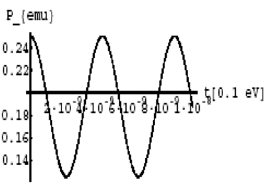
Figure 5: $P_{e\mu}$ as function of $t$ within $A=B=0.1\ \textrm{eV},C=d=s=0$.

The figure shows that, if $A$ and $B$ are taken in order 0.1 eV (upper cosmological bound) we have solar neutrino data for $t$ parameter.

For the $\nu_{e}\nu_{\mu}$ transition in matter, ignoring magnetic field, we get typical terms similar to that in Ref.kl . For general case, $P_{\alpha\beta}$ cannot be cast in compact form and may require numerical evaluation. Analysis of the matter effect is quite simple in the case of two generations and gives a result in good agreement with the current evaluation.

VI Summary and Conclusions

The basic motivation of this work is to study neutrino mass and mixing in the framework of the model based on $\mbox{SU}(3)_{C}\otimes\mbox{SU}(3)_{L}\otimes\mbox{U}(1)_{X}$ gauge group with right-handed neutrinos.

The Higgs sector of this model contains the bilepton Higgs scalars with lepton number $L=2$. Hence, the Yukawa coupling of the model has automatic lepton number symmetry which is broken only by the self-couplings of the Higgs boson. The interesting radiative mechanism for neutrino masses has been obtained. At the tree level, the neutrino spectrum contains three Dirac fermions, one massless and two degenerate in mass. At the two-loop level, neutrinos obtain Majorana masses and correct the tree-level result which naturally gives rise to the pseudo-Dirac mass differences and an inverted hierarchy mass pattern and interesting mixing which can fit the current data with minor fine-tuning.

For the solar neutrino oscillations in matter, neglecting magnetic field, we have got the matter effects. Our analysis in the simpler case limited by two generations shows that the scheme gives appropriate consistency.

In another scenarios, one can pick the scales such that the loop-induced Majorana mass matrix is bigger than the Dirac one and thus reproduce the usual seesaw mechanism.

The complete analysis and study of the astrophysics constraint, the medium effects will be investigated in the future works.

Appendix A Diagonalization of the mass matrix

Let us consider a free case

$$H_{0}=\left(\begin{array}[]{cc}0&M\\ M^{T}&0\end{array}\right),$$ (154)

where $M^{T}=-M,\hskip 14.22636ptM^{*}=M$ and

$$M=\left(\begin{array}[]{ccc}0&A&B\\ -A&0&C\\ -B&-C&0\end{array}\right)$$ (158)

The interaction is considered as perturbation $V=\left(\begin{array}[]{cc}0&0\\ 0&\Delta\end{array}\right),$ with $\Delta=\left(\begin{array}[]{ccc}0&d&s\\ d&0&t\\ s&t&0\end{array}\right).$ Let us start with a simple case $\Delta=0$ then $H=H_{0}+V=\left(\begin{array}[]{cc}0&M\\ -M&0\end{array}\right).$ We search eigenvectors in the form $\Psi_{E}=\left(\begin{array}[]{c}\varphi_{A}\\ \varphi_{B}\end{array}\right)$ satisfied the equation $H\Psi_{E}=E\Psi_{E}$. Then we obtain an equation

$$\left(\begin{array}[]{cc}0&M\\ -M&0\end{array}\right)\left(\begin{array}[]{c}\varphi_{A}\\ \varphi_{B}\end{array}\right)=E\left(\begin{array}[]{c}\varphi_{A}\\ \varphi_{B}\end{array}\right)$$ (164)

Equivalently,

$$M\varphi_{B} = E\varphi_{A},$$

$$-M\varphi_{A} = E\varphi_{B}.$$ (165)

From Eq. (165), we get $-M^{2}\varphi_{A}=EM\varphi_{B}=E^{2}\varphi_{A},$ or $(-M^{2})\varphi_{A}=E^{2}\varphi_{A}$. This means that we need only to diagonalize $M$. Next, we consider a characteristic equation

$$\left(\begin{array}[]{ccc}-\lambda&A&B\\ -A&-\lambda&C\\ -B&-C&-\lambda\end{array}\right)=0$$ (169)

or $\lambda(\lambda^{2}+A^{2}+B^{2}+C^{2})=0.$ Thus, we get three roots : $\lambda=0,\ \pm i\sqrt{A^{2}+B^{2}+C^{2}}$. Let us denote $L=\sqrt{A^{2}+B^{2}+C^{2}}$, then

$$E^{2}=-\lambda_{i}^{2}=0,\ -(\pm iL)^{2}=0,\ L^{2},\hskip 14.22636ptL^{2}$$ (170)

Thus we have three eigenvalues : $+iL,\ 0,\ -iL$. Let us choose $\varphi_{A}$ to be $M^{\prime}s$ eigenstate

$$\left(\begin{array}[]{ccc}0&A&B\\ -A&0&C\\ -B&-C&0\end{array}\right)\left(\begin{array}[]{c}x\\ y\\ z\end{array}\right)=0$$ (177)

It is easily to get $\left(\begin{array}[]{c}x\\ y\\ z\end{array}\right)=\left(\begin{array}[]{c}-C\\ B\\ -A\end{array}\right).$ Let us change a sign of the eigenstate $\left(\begin{array}[]{c}-C\\ B\\ -A\end{array}\right)\rightarrow\left(\begin{array}[]{c}C\\ -B\\ A\end{array}\right).$ Thus, we get a massless eigenstate $|\ 0\ \rangle=\frac{1}{L}\left(\begin{array}[]{c}C\\ -B\\ A\end{array}\right).$ Now we look for other eigenstates

$$\left(\begin{array}[]{ccc}0&A&B\\ -A&0&C\\ -B&-C&0\end{array}\right)\left(\begin{array}[]{c}x\\ y\\ z\end{array}\right)=\pm iL\left(\begin{array}[]{c}x\\ y\\ z\end{array}\right)$$ (187)

or $Ay+Bz=(\pm iL)x$ and $-Ax+Cz=(\pm iLy)$ or $\pm iLx-Ay=Bz$ and $Ax\pm iLy=Cz$. We get then,

$$\left(\frac{BC-iAL}{AB+iCL},\hskip 14.22636pt\frac{A^{2}+C^{2}}{AB+iCL},\hskip 14.22636pt1\right)$$ (188)

for $\lambda=iL$, and

$$\left(\frac{-BC-iAL}{-AB+iCL},\hskip 14.22636pt-\frac{A^{2}+C^{2}}{-AB+iCL},\hskip 14.22636pt1\right)$$ (189)

for $\lambda=-iL$. Thus the normalized eigenstates are given by

$$|\ \phi_{+}\ \rangle^{T} = \frac{1}{\sqrt{2(A^{2}+C^{2})(A^{2}+B^{2}+C^{2})}}(BC-iAL,A^{2}+C^{2},AB+iCL),$$ (190)

$$|\ \phi_{-}\ \rangle^{T} = \frac{1}{\sqrt{2(A^{2}+C^{2})(A^{2}+B^{2}+C^{2})}}(BC+iAL,A^{2}+C^{2},AB-iCL)$$ (191)

Now we have obtained three eigenstates $|\ \phi_{0}\ \rangle,\ |\ \phi_{+}\ \rangle,\ |\ \phi_{-}\ \rangle$. It is straightforward to check that they form an orthonormal basis. Note that, for an anti-Hermitian matrix like $M$, its eigenstates (with different $E$) are also orthogonal!

Now, it is straightforward to construct the eigenstates of the true Hamiltonian $H$. For $E\neq 0$, Eq. (165) gives

$$\varphi_{B}=-\frac{1}{E}M\varphi_{A}$$ (192)

1. For $E=L$: $\varphi_{B}=-\frac{1}{L}M\varphi_{A}$. Taking $\varphi_{A}=\phi_{+}$, then $\varphi_{B}=-\frac{i}{L}L\phi_{+}=-i\phi_{+}$. Thus we have $\Psi_{1}=\frac{1}{\sqrt{2}}\left(\begin{array}[]{c}\phi_{+}\\ -i\phi_{+}\end{array}\right)$. Similarly, let $\varphi_{A}=\phi_{-}$, then $\varphi_{B}=-\frac{1}{L}(-iL)\phi_{-}=i\phi_{-}$. Hence $\Psi_{2}=\frac{1}{\sqrt{2}}\left(\begin{array}[]{c}\phi_{-}\\ i\phi_{-}\end{array}\right)$. Note that $\langle\Psi_{1}|\Psi_{2}\rangle=\frac{1}{2}(\phi^{+}_{+},i\phi^{+}_{+})\left(\begin{array}[]{c}\phi_{-}\\ i\phi_{-}\end{array}\right)=\phi^{+}_{+}\phi_{-}(1-1)=0$.

2. For $E=-L$: $\varphi_{B}=\frac{1}{L}M\varphi_{A}$. Analogously, we get $\Psi_{5}=\frac{1}{\sqrt{2}}\left(\begin{array}[]{c}\phi_{+}\\ i\phi_{+}\end{array}\right)\hskip 14.22636pt{\rm and}\hskip 14.22636pt\Psi_{6}=\frac{1}{\sqrt{2}}\left(\begin{array}[]{c}\phi_{-}\\ -i\phi_{-}\end{array}\right).$

3. For $E=0$: a special case $\Psi_{3}=\left(\begin{array}[]{c}\phi_{0}\\ 0\end{array}\right)\hskip 14.22636pt{\rm and}\hskip 14.22636pt\Psi_{4}=\left(\begin{array}[]{c}0\\ \phi_{0}\end{array}\right).$

Now we only need to rewrite the perturbation $V$ in a new basis

$$V_{ij}=\langle\Psi_{i}|V|\Psi_{j}\rangle,\hskip 14.22636pti,j=1,2,...,6,\hskip 14.22636ptV=\left(\begin{array}[]{cc}0&0\\ 0&\Delta\end{array}\right).$$ (195)

We also have $\Delta=\sum_{i,j}|\phi_{i}\rangle\Delta_{ij}\langle\phi_{j}|.$ Sine $\Psi_{i}$ are expressed through just three functions $\phi_{+},\ \phi_{0},\ \phi_{-}$, so we only need to work out the $3\times 3$ matrix! Finally, the $6\times 6$ matrix is

$$\left(\begin{array}[]{cccccc}\frac{1}{2}\Delta_{++}&-\frac{1}{2}\Delta_{+-}&0&\frac{i}{\sqrt{2}}\Delta_{+0}&-\frac{1}{2}\Delta_{++}&\frac{1}{2}\Delta_{+-}\\ -\frac{1}{2}\Delta_{-+}&\frac{1}{2}\Delta_{--}&0&-\frac{i}{\sqrt{2}}\Delta_{-0}&-\frac{1}{2}\Delta_{-+}&-\frac{1}{2}\Delta_{--}\\ 0&0&0&0&0&0\\ -\frac{i}{\sqrt{2}}\Delta_{0+}&\frac{i}{\sqrt{2}}\Delta_{0-}&0&\Delta_{00}&\frac{i}{\sqrt{2}}\Delta_{0+}&-\frac{i}{\sqrt{2}}\Delta_{0-}\\ -\frac{1}{2}\Delta_{++}&\frac{1}{2}\Delta_{+-}&0&-\frac{i}{\sqrt{2}}\Delta_{+0}&\frac{1}{2}\Delta_{++}&-\frac{1}{2}\Delta_{+-}\\ \frac{1}{2}\Delta_{-+}&-\frac{1}{2}\Delta_{--}&0&\frac{i}{\sqrt{2}}\Delta_{-0}&-\frac{1}{2}\Delta_{-+}&\frac{1}{2}\Delta_{--}\end{array}\right)$$ (202)

To calculate the leading corrections, only need to diagonalize the $2\times 2$ matrix. Note that $\Delta_{ij}=\Delta_{ij}(d,s,t)$ are homogeneous function of order 1 for $(d,s,t)$. The matrix $\left(\begin{array}[]{cc}0&0\\ 0&\Delta_{00}\end{array}\right)$, gives $\Delta E=0,\ \Delta_{00}+{\cal O}(g^{2})$. which is analytic function. So, the energy spectra for $E_{3},E_{4}$ are given

$$E_{3} = 0+{\cal O}(g^{2}),\ E_{4}=\Delta_{00}+{\cal O}(g^{2})$$ (203)

Next, the matrix $\left(\begin{array}[]{cc}\frac{1}{2}\Delta_{++}&-\frac{1}{2}\Delta_{+-}\\ -\frac{1}{2}\Delta_{-+}&\frac{1}{2}\Delta_{--}\end{array}\right),$ has two eigenvalues given by

$$\Delta E=\frac{\Delta_{++}+\Delta_{--}}{4}\pm\sqrt{\left(\frac{\Delta_{++}-\Delta_{--}}{4}\right)^{2}+\frac{|\Delta_{+-}|^{2}}{4}}$$ (204)

which is, in general, nonanalytic!. For instance, $f(d,s,t)=\sqrt{d^{2}+s^{2}+t^{2}}$ is not analytic at $(d,s,t)=(0,0,0)$. Thus, we obtain

$$E_{1,2} = L+\frac{\Delta_{++}+\Delta_{--}}{4}\pm\sqrt{\left(\frac{\Delta_{++}-\Delta_{--}}{4}\right)^{2}+\frac{|\Delta_{+-}|^{2}}{4}}+{\cal O}(g^{2}),$$ (205)

$$E_{5,6} = -L+\frac{\Delta_{++}+\Delta_{--}}{4}\pm\sqrt{\left(\frac{\Delta_{++}-\Delta_{--}}{4}\right)^{2}+\frac{|\Delta_{+-}|^{2}}{4}}+{\cal O}(g^{2})$$ (206)

The ${\cal O}(g)$ corrections are nonanalytic in general!. To get explicit results we calculate $\Delta_{ij}$.
$\Delta_{++}=\phi_{+}^{+}\Delta\phi_{+}=\frac{1}{2(A^{2}+C^{2})L^{2}}\\ \times(BC+iAL,A^{2}+C^{2},AB-iCL)\left(\begin{array}[]{ccc}0&d&s\\ d&0&t\\ s&t&0\end{array}\right)\left(\begin{array}[]{c}BC-iAL\\ A^{2}+C^{2}\\ AB+iCL\end{array}\right)=\frac{1}{L^{2}}(BCd-ACs+ABt).$ Noting $\phi_{-}=\phi_{+}^{*}$, we have $\Delta_{--}=\Delta_{++}$.

Now we turn our attention to $\Delta_{00}$. $\Delta_{00}=\phi_{0}^{+}\Delta\phi_{0}=\frac{1}{L^{2}}(C,-B,A)\left(\begin{array}[]{ccc}0&d&s\\ d&0&t\\ s&t&0\end{array}\right)\left(\begin{array}[]{c}C\\ -B\\ A\end{array}\right)=-\frac{2}{L^{2}}(BCd-ACs+ABt)=-2\Delta_{++}$.
$\Delta_{+-}=\phi_{+}^{+}\Delta\phi_{-}=\frac{1}{2(A^{2}+C^{2})L^{2}}\times(BC+iAL,A^{2}+C^{2},AB-iCL)\left(\begin{array}[]{ccc}0&d&s\\ d&0&t\\ s&t&0\end{array}\right)\left(\begin{array}[]{c}BC+iAL\\ A^{2}+C^{2}\\ AB-iCL\end{array}\right)=\left(\frac{BC+iAL}{L^{2}}\right)d+\left[\frac{AC(B^{2}+L^{2})-iBL(C^{2}-A^{2})}{(A^{2}+C^{2})L^{2}}\right]s+\left(\frac{AB-iCL}{L^{2}}\right)t$.

We have $\Delta_{-+}=(\Delta_{+-})^{*}$. Similarly $\Delta_{0+}=\phi_{0}^{+}\Delta\phi_{+}=\left[\frac{C(L^{2}-2B^{2})+iABL}{\sqrt{2(A^{2}+C^{2})}L^{2}}\right]d+\left[\frac{2ABC+iL(C^{2}-A^{2})}{\sqrt{2(A^{2}+C^{2})L^{2}}}\right]s+\left[\frac{A(L^{2}-2B^{2})-iLBC}{\sqrt{2(A^{2}+C^{2})L^{2}}}\right]t,$ and
$\Delta_{0-}=\phi_{0}^{+}\Delta\phi_{-}=\left[\frac{C(L^{2}-2B^{2})-iABL}{\sqrt{2(A^{2}+C^{2})}L^{2}}\right]d+\left[\frac{2ABC-iL(C^{2}-A^{2})}{\sqrt{2(A^{2}+C^{2})L^{2}}}\right]s+\left[\frac{A(L^{2}-2B^{2})+iLBC}{\sqrt{2(A^{2}+C^{2})L^{2}}}\right]t$.

Noting that $\phi_{0}$ is real, and $\phi_{+}=\phi_{-}^{*}$, we have the following properties $\Delta_{0-}=\Delta_{0+}^{*}=\Delta_{-0}^{*}=\Delta_{+0}$. To complete, we calculate

$$|\Delta_{+-}|^{2} = \frac{1}{L^{4}(A^{2}+C^{2})^{2}}\left\{(A^{2}+C^{2})^{2}[(B^{2}C^{2}+A^{2}L^{2})d^{2}+(A^{2}B^{2}+C^{2}L^{2})t^{2}\right.$$ (207)

$$- 2(A^{2}+C^{2})ACdt]+(A^{2}B^{2}+C^{2}L^{2})(B^{2}C^{2}+A^{2}L^{2})s^{2}$$

$$+ \left.2(A^{2}+C^{2})[(B^{2}C^{2}+A^{2}L^{2})ABds+(A^{2}B^{2}+C^{2}L^{2})BCst]\right\}$$

References

• (1) SuperKamiokande Collaboration, Y. Fukuda et al., Phys. Rev. Lett. 81, 1562 (1998); Y. Ashie et al, Phys. Rev. Lett. 93, 101801 (2004); [arXiv:hep-ex/0510064].
• (2) KamLAND Collaboration, K. Eguchi et al., Phys. Rev. Lett. 90, 021802 (2003); T. Araki et al, Phys. Rev. Lett. 94, 081801(2005).
• (3) SNO Collaboration, Q. R. Ahmad et al., Phys. Rev. Lett. 89, 011301 (2002); Phys. Rev. Lett. 89, 011302 (2002); Phys. Rev. Lett. 92, 181301 (2004); B. Aharmim et al, Phys. Rev. C 72, 055502 (2005) [arXiv:nucl-ex/0502021].
• (4) For a brief review, see A. Yu. Smirnov, [arXiv:hep-ph/0402264]; G. Altarelli, Nucl. Phys. B, Proc. Suppl. 143, 470 (2005) [arXiv:hep-ph/0410101].
• (5) M. Maltoni et al., Phys. Rev. D68 (2003) 113010.
• (6) G. L. Fogli, E. Lisi, A. Marrone, and A. Palazzo, [arXiv: hep-ph/0506083].
• (7) Ch. Weinheimer, Proceedings of the 20th International Conference on Neutrino Physics and Astrophysics, Neutrino 2002 (Munich, Germany) May 25-30, 2002, Nucl. Phys. Proc. Suppl. 118, 388 (2003)[arXiv:astro-ph/0209556]; V. Lobashev et al, Nucl. Phys. Proc. Suppl. 91 (2001) 280.
• (8) M. Tegmark et al, Phys. Rev. D 69 (2004) 103501.
• (9) F. Pisano and V. Pleitez, Phys. Rev. D 46, (1992) 410; P. H. Frampton, Phys. Rev. Lett. 69, (1992) 2889; R. Foot et al, Phys. Rev. D 47, (1993) 4158.
• (10) M. Singer, J. W. F. Valle, and J. Schechter, Phys. Rev. D 22, (1980) 738; R. Foot, H. N. Long, and Tuan A. Tran, Phys. Rev. D 50, (1994) R34; J. C. Montero, F. Pisano, and V. Pleitez, Phys. Rev. D 47, (1993) 2918; H. N. Long, Phys. Rev. D 53, (1996) 437; Phys. Rev. D 54, (1996) 4691.
• (11) W. A. Ponce, D. A. Gunierrez and L. A. Sanchez, Phys. Rev. D 69 (2004) 055007; A. G. Dias and V. Pleitez, Phys. Rev. D 69 (2004) 077702; G. Tavares-Velasco and J. J. Toscano, Phys. Rev. D 65, 013005 (2004); Phys. Rev. D 70, 053006 (2004); G. A. Gonzales-Sprinberg, R. Martinez, and O. Sampayo, Phys. Rev. D 71, 115003 (2005); L. D. Ninh and H. N. Long, Phys. Rev. D 72, 075004 (2005); D. Anderson and M. Sher, Phys. Rev. D 72, 095014 (2005).
• (12) H. N. Long and T. Inami, Phys. Rev. D 61 (2000) 075002.
• (13) Y. Okamoto and M. Yasue, Phys. Lett. B 466, 267 (1999).
• (14) T. Kitabayshi and M. Yasue, Phys. Rev. D63 (2001) 095002; Phys. Rev. D63 (2001) 095006; Nucl. Phys. B 609 (2001) 61; Phys. Rev. D 67 (2003) 015006.
• (15) Recent works in this direction are: J. C. Montero, C. A. de S. Pires and V. Pleitez, Phys. Rev. D65 (2002) 095001; A. A. Gusso, C. A. de S. Pires and P. S. Rodrigues da Silva, Mod. Phys. Lett. A 18 (2003) 1849; I. Aizawa, et al, Phys. Rev. D 70, (2004) 015011.
• (16) A. Zee, Phys. Lett. B93, 389 (1980); B161, 141 (1985); Nucl. Phys. B264, 99 (1986); L. Wolfenstein, Nucl. Phys. B175, 93 (1980); K. S. Babu, Phys. Lett. B 203, 132 (1988); D. Chang, W.-Y. Keung, and P. B. Pal, Phys. Rev. Lett. 61, 2420 (1988); J. T. Peltonieri, A. Yu. Smirnov, and J. W. Valle, Phys. Lett. B 286, 321 (1992); D. Choodhury, R. Gandhi, J. A. Gracey, and B. Mukhopadhyaya, Phys. Rev. D50, 3468 (1994).
• (17) D. Chang and A. Zee, Phys. Rev. D 61 (2000) 071303 (R); C. Jarlskog, M. Matsuda, S. Skalhauge and M. Tanimoto, Phys. Lett. B 449 (1999) 240
• (18) L. Wolfenstein, Nucl. Phys. B186 (1981) 147; D. Chang and O. Kong, Phys. Lett. B477 (2000) 416.
• (19) M. Kobayashi and C. S. Lim, Phys. Rev. D64 (2001) 013003.
• (20) J. F. Beacom, et al, Phys. Rev. Lett. 92 (2004) 011101.
• (21) M. B. Tully and G. C. Joshi, Int. J. Mod. Phys. A13 (1998) 5593.
• (22) M. B. Tully and G. C. Joshi, Phys. Rev. D64, (2001) 011301(R).
• (23) R. A. Diaz, R. Martinez, and F. Ochoa, Phys. Rev. D69 (2004) 095009, [arXiv: hep-ph/0309280].
• (24) A. G. Dias, C. A. de S. Pires and P. S. Rodriguez da Silva, Phys. Lett. B 628, (2005) 85, [arXiv: hep-ph/0508186].
• (25) N. Okada and O. Yasuda, Int. J. Mod. Phys. A 12 (1997) 3669; S. M. Bilenky, C. Giunti, W. Grimus, and Schwetz, Astropart. Phys. 11 (1999) 413; K. N. Abazajian, Astropart. Phys. 19 (2003) 303.
• (26) G. Gelmini, S. P. Ruiz, and S. Pascoli, Phys. Rev. Lett. 93 (2004) 081302; see also R. H. Cyburt, B. D. Fields, K. A. Olive, and E. Skillman, Astropart. Phys. 23 (2005) 313.
• (27) T. K. Kuo and J. T. Pantaleone, Rev. Mod. Phys. 61, (1989) 937; R. N. Mohapatra and P. B. Pal, Massive Neutrinos in Physics and Astrophysics, (World Scientific 2004).
• (28) See for example, S. M. Bilenky, [arXiv: hep-ph/0402153].