Interactions of multi-quark states in the chromodielectric model

Abstract

We investigate 4-quark ($qq\bar{q}\bar{q}$) systems as well as multi-quark states with a large number of quarks and anti-quarks using the chromodielectric model. In the former type of systems the flux distribution and the corresponding energy of such systems for planar and non-planar geometries are studied. From the comparison to the case of two independent $q\bar{q}$-strings we deduce the interaction potential between two strings. We find an attraction between strings and a characteristic string flip if there are two degenerate string combinations between the four particles. The interaction shows no strong Van-der-Waals forces and the long range behavior of the potential is well described by a Yukawa potential, which might be confirmed in future lattice calculations. The multi-quark states develop an inhomogeneous porous structure even for particle densities large compared to nuclear matter constituent quark densities. We present first results of the dependence of the system on the particle density pointing towards a percolation type of transition from a hadronic matter phase to a quark matter phase. The critical energy density is found at $\varepsilon_{c}=1.2\,\text{GeV}/\text{fm}^{3}$.

I Introduction

Quantum Chromodynamics (QCD) is the theory for color charged quarks and gluons. This theory has been tested successfully in the regime of large momentum transfer such as in deep inelastic scattering, where perturbative methods can be used due to asymptotic freedom. It is a common belief that QCD should be able to describe all systems ruled by strong interactions. These cover a wealth of different regimes ranging from the dynamics of quasi free quarks and gluons in a quark gluon plasma (QGP) at high temperatures or densities, over the formation of hadrons out of quarks to the interactions between those color neutral hadrons. However, in this latter region of small relative momenta, where the confinement phenomenon plays a dominant role, no convincing analytical techniques have been established yet. The only calculations from first principles are restricted to QCD lattice simulations, where the results are limited due to today’s computing power.

Therefore one still has to rely on models, that describe the interactions between quarks and gluons bound to hadrons phenomenologically and that include confinement. Such models are for example the well known MIT bag model Chodos et al. (1974a, b), where quarks are confined by a given external cavity or the quark molecular dynamics model, Hofmann et al. (2000); Scherer et al. (2001); Akimura et al. (2005), where quarks follow the Hamiltonian dynamics subject to a linear rising potential between quarks ($q$) and anti-quarks ($\bar{q}$). Another approach is the model of the dual super conductor known also dual Abelian Higgs model or dual Ginzburg-Landau model Baker et al. (1991); Ripka (2004) where confinement is achieved by monopole condensation ’t Hooft (1974); Polyakov (1974) and an accompanying magnetic supercurrent. The model of the stochastic vacuum relies on the calculation of Wilson loops in a Gaussian approximation Dosch (1987); Kuzmenko and Simonov (2001); Shoshi et al. (2003) which leads to a linearly rising $q\bar{q}$-potential.

In this work we choose the framework of the chromodielectric model (CDM) Friedberg and Lee (1977a, b); Wilets (1989). Unlike the MIT bag model, CDM has the benefit, that bags with a smooth surface are created self-consistently and dynamically out of the underlying field equations, due to the presence of colored quarks.

The CDM has already been used to calculate properties of the nucleon and its low lying resonances like masses, magnetic moments and the axial-vector/vector coupling constant ratio Goldflam and Wilets (1982). In Bickeböller et al. (1985); Grabiak and Gyulassy (1991); Martens et al. (2003) a description of $q\bar{q}$-strings was given, and in Martens et al. (2004) the parameters of the CDM were adjusted to reproduce results of lattice calculations Bali et al. (1995, 1997). In the same work, the flux tube structure of a baryon like $qqq$-bag has been studied. Further, within the model, the interactions between $q\bar{q}$-strings Loh et al. (1997a) and the nucleon-nucleon interaction in vacuum and in nuclear matter Pirner et al. (1984); Achtzehnter et al. (1985); Schuh et al. (1986); Koepf et al. (1994); Pepin et al. (1996) has been discussed. In another approach the model has been used in a transport theoretical framework to describe the dynamics of quarks bound in nucleons and strings Kalmbach et al. (1993); Vetter et al. (1995). In Loh et al. (1997b) the disintegration of $q\bar{q}$-pairs in strong color electric fields has been observed. A full molecular dynamical simulation of hadronization out of a gas of quarks and gluons has been presented in Traxler et al. (1999).

In this paper we will analyze the interactions between the color electric flux tubes for a wide class of different quark configurations. In a previous paper Martens et al. (2004) we have given the structure of meson like $q\bar{q}$-states and baryon like $qqq$ states. The model has been successfully adjusted to reproduce lattice results for both the $q\bar{q}$-potential and the transverse shape of the flux tubes. It is an open question, how the flux tubes of the basic white two- and three-particle clusters interact with each other. In order to understand the interactions we extend our previous analysis to configurations with more than three particles. The easiest of such systems, the $qq\bar{q}\bar{q}$-system, already develops two distinct bags, that may interact with each other. We can study those systems for different spatial quark configurations. Besides this, the system is still simple enough to be treated on the lattice. In fact there are lattice results for the four-particle system in SU(2) Green et al. (1993) and also in SU(3) Okiharu et al. (2005a). Where possible, we will compare our results with those obtained on the lattice. Knowing the interactions between the flux tubes of color neutral objects, it is an interesting issue, how this interaction governs the transition from a system of distinct white hadrons to a system of interacting colored quarks in a quark plasma. It is an old prediction of QCD, that there is a rapid transition for increasing temperature Karsch et al. (2000). This transition to the quark gluon plasma (QGP) has been explicitly seen for vanishing baryon chemical potential as a steep rise of the thermodynamic pressure of the system at a temperature $T=(170\text{-}180)\,$MeV Karsch et al. (2001). For non-zero baryo-chemical potential, lattice calculations suffer from technical problems and cannot be easily performed up to now. See Fodor and Katz (2004a, b), where the transition temperature was explored for small chemical potential. However, for increasing baryon densities one expects that the hadrons start to overlap and the quarks are free over a much larger volume and a transition to a quark gas might occur as well. In contrast, in our treatment of the CDM we have only static configurations and therefore we do not describe quark systems at non-zero temperature. But it is possible to vary the quark density and study many-quark systems and the behavior of the very dense flux tubes.

The paper is organized in the following way. In section II we introduce briefly the chromodielectric model, give the equations of motion for the underlying fields as well as the corresponding field energies. We solve these equations numerically in three spatial dimensions. We also discuss the color structure of the model and its connection to the SU(3) color algebra. Section III is devoted to the long range behavior of fields of $q\bar{q}$-strings, which extends the discussion of the bulk properties of strings in Martens et al. (2004). We will show the characteristic exponential decay of all fields with the distance from the string center. In section IV we show the interactions between two $q\bar{q}$-strings of various lengths and with relative orientations to each other. We first show our results for the color electric fields in section IV.1 and the distribution of the energy density in section IV.2. The distortion of the one $q\bar{q}$-string under the influence of the other one is shown explicitly. For simplicity, we concentrate on the discussion of strings that are parallel or anti-parallel to each other. In this case, all particles are lying in a single plane. However, as the calculations are done in three dimensions, we are able to study particle configurations too, that are extended in three space dimensions. We will show the results of the calculations for these tetrahedronic configurations as well. In section IV.3 we give the interaction potential of the two strings as calculated from field energies. Again we concentrate on the potential for plane configurations but we will discuss also a wide range of 3-dimensional configurations. We will extract the static string interaction potential which can be compared to lattice calculations. In section V we present first results on static multi-particle systems. We show the heterogeneous structure of the emerging flux tubes and analyze the scaling of the multi-quark properties with the particle density. A qualitative description of the deconfinement phase transition is given. Finally we discuss our results in section VI and give our summary.

II The chromodielectric model

As there is no confinement in quantum electrodynamics, one believes that confinement is due to the non-Abelian nature of QCD. Although the detailed mechanism of confinement has not been revealed within QCD, there is strong evidence for it from lattice QCD. The most prominent result is the linear rising potential between a static quark anti-quark pair at zero temperature Bali and Schilling (1992); Deldar (2000) and at finite temperature Bornyakov et al. (2004). In addition, the formation of long, string like flux tubes between a $q\bar{q}$-pair has been seen both in SU(3) Matsubara et al. (1994); Ichie et al. (2003) and in SU(2) Bali et al. (1995), where the results are much more precise for numerical reasons. Despite the fact that the structure of the QCD vacuum is highly complicated, its long range behavior might be transparent. In the CDM it is assumed that this vacuum behaves as a perfect dielectric medium described by a vanishing dielectric constant $\kappa_{\text{vac}}$. Dual to a normal superconductor, where magnetic fields are expelled from the superconducting phase, in CDM the color electric fields are expelled from the QCD vacuum. In the presence of color charged quarks, the resulting color fields are compressed into flux tube like excitations of the vacuum. In Mack (1984); Pirner et al. (1984); Pirner (1992) a renormalization group derivation was given for the lattice colordielectric model, which has a scalar confinement field, and keeps strongly coupled non-Abelian fields in the large distance limit. CDM is formulated in terms of two Abelian color fields $A^{\mu,a}$ only and an additional scalar confinement field $\sigma$. This scalar field is designed to already include the non-Abelian effects of the gluon sector. There are indications that in the long range limit only the Abelian components contribute to the observable quantities: ’t Hooft suggested in ’t Hooft (1974) the maximal Abelian gauge for projecting out a Cartan subgroup believed to be relevant for infrared aspects of QCD. In Ezawa and Iwazaki (1982); Kronfeld et al. (1987); Amemiya and Suganuma (1999) further support for the Abelian dominance was found due to the mass generation of off-diagonal gluons. In Shiba and Suzuki (1994); Bali et al. (1996) the string tension in the Abelian approximation was reproduced within some percent deviation from the full value.

Following this reasoning, CDM is formulated in a Cartan subgroup of QCD reducing the independent color fields to a set of two commuting field $A^{\mu,a}$ with $a\in\{3,8\}$. These two fields are connected to the Gell-Mann matrices $\lambda^{3,8}$ which commute with each other in the standard representation. Confining effects are merged into the dielectric coupling of these gluon fields to the dielectric medium generated by the confinement field $\sigma$. The CDM Lagrange density can now be given as

$${\cal L} = {\cal L}_{g}+{\cal L}_{\sigma}\quad,$$ (1a)

$${\cal L}_{g} = -{\textstyle\frac{1}{4}}{\kappa(\sigma)}F_{\mu\nu}^{a}F^{\mu\nu,{a}}-g_{s}\;j_{\mu}^{a}\,A^{\mu,a}\quad,$$ (1b)

$${\cal L}_{\sigma} = {{\textstyle\frac{1}{2}}\partial_{\mu}\sigma\partial^{\mu}\sigma-U(\sigma)}\quad,$$ (1c)

$$F^{\mu\nu,{a}} = \partial^{\mu}A^{\nu,a}-\partial^{\nu}A^{\mu,a},\;\;\;a\in\{3,8\}\quad,$$ (1d)

where $A^{\mu,a}=(\phi^{a},\vec{A}^{a})$ is composed out of the color electrostatic potential $\phi^{a}$ and the vector potential $\vec{A}^{a}$.

In the following we are interested especially in the interactions of the electric flux tubes, thus we have omitted the dynamic term for the quark degrees of freedom. Quarks enter into the model only via the external color current $j^{\mu,a}=(\rho^{a},\vec{\jmath}^{\,a})$ with a coupling strength $g_{s}$. Furthermore we treat the quarks as infinitely heavy, static sources. Therefore the color current vanishes $\vec{\jmath}^{\,a}=0$. The color charge density $\rho^{a}(\vec{x})=\sum_{k}q_{k}^{a}w(\vec{x}-\vec{x}_{k})$ is given as a sum over all quarks with two color charges $q^{a}$ and a spatial distribution $w(\vec{x})$. In principle the quarks are point-like objects, but for numerical reasons we assign a Gaussian distribution $w(\vec{x})=(2\pi r_{0}^{2})^{-3/2}\exp(-\vec{x}^{2}/2r_{0}^{2})$ with a small width $r_{0}=0.02\,\text{fm}$, which is on the order of the spacing of the numerical grid used in the calculations. The grid spacing chosen is small compared to all physical sizes like the flux tube radius.

In the Abelian approximation the quarks still have three different colors. These are expressed as three dimensional unit vectors in the fundamental representation of color space as $|c\rangle\in\{|r\rangle,|g\rangle,|b\rangle\}$. The color charges are then given by the diagonal entries of the corresponding generators $t^{a}=\lambda^{a}/2$, i.e. $q^{a}=\langle c|t^{a}|c\rangle$. Formulated differently, the two color charges $(q^{3},q^{8})$ are given by the weight vectors of QCD Scherer et al. (2001). The numerical values of the color charges can be read off from table 1 and are depicted in figure 1.

color	$q^{3}$	$q^{8}$
red	$1/2$	$1/(2\sqrt{3})$
green	$-1/2$	$1/(2\sqrt{3})$
blue	$0$	$-1/\sqrt{3}$

Table 1: The color charges $q^{a}$ of the three colors with respect to the two Abelian color fields. The charge of the anti-colors are given by the negative of the color charges.

Figure 1: The color charge $(q^{3},2\sqrt{3}q^{8})$ with respect to the color fields $A^{3,8}$ for the three colors $r,g,b$.

The model inherits a U(1)$\times$U(1) gauge symmetry and a global symmetry corresponding to finite rotations in color space Martens et al. (2004) which is a remnant of the original SU(3) symmetry of QCD. Only the Lagrange density and the energy density, which is stated explicitly later on, are invariant under these rotations but not the color fields themselves.

The color field tensor $F^{\mu\nu,a}$ ($a\in\{3,8\}$) in Eq. (1d) defines the color electric and magnetic fields $\vec{E}_{i}^{a}=-F^{0i,a}=\left(-\nabla\phi^{a}-\partial_{t}\vec{A}^{a}\right)_{i}$ and $\vec{B}_{i}^{a}=-{\textstyle\frac{1}{2}}\varepsilon_{ijk}F^{jk,a}=(\nabla\times\vec{A}^{a})_{i}$ respectively. With the definition of the medium fields $\vec{D}^{a}=\kappa(\sigma)\vec{E}^{a}$ and $\vec{H}^{a}=\kappa(\sigma)\vec{B}^{a}$ the equations of motion following from Eq. (1) are given by

$$\nabla\cdot\vec{D}^{a} = g_{s}\rho^{a}\quad,$$ (2a)

$$\nabla\times\vec{H}^{a}-\partial_{t}\vec{D}^{a} = g_{s}\vec{\jmath}^{\;a}\quad,$$ (2b)

$$\nabla\times\vec{E}^{a}+\partial_{t}\vec{B}^{a} = 0\quad,$$ (2c)

$$\nabla\cdot\vec{B} = 0\quad,$$ (2d)

$$\left(\partial_{t}^{2}-\vec{\nabla}^{2}\right)\sigma+U^{\prime}(\sigma) = -{\textstyle\frac{1}{4}}\kappa^{\prime}(\sigma)F_{\mu\nu}^{a}F^{\mu\nu,a}\quad.$$ (2e)

With $\vec{\jmath}^{\;a}=0$ and the assumptions that all time derivatives vanish exactly and $\vec{A}^{a}=0$, the magnetic field is $\vec{B}^{a}=0$ and the equations of motion (e.o.m.) can be cast into the following form:

$$\nabla\cdot(\kappa(\sigma)\nabla\phi^{a}) = -g_{s}\rho^{a}\quad,$$ (3a)

$$\nabla^{2}\sigma-U^{\prime}(\sigma) = -\frac{1}{2}\frac{\kappa^{\prime}(\sigma)}{\kappa^{2}(\sigma)}\vec{D}^{a}\cdot\vec{D}^{a}\quad.$$ (3b)

The energy of the system for static configurations is given by

$$E_{\text{tot}} = E_{\text{el}}+E_{\text{vol}}+E_{\text{sur}}\quad,$$ (4a)

$$E_{\text{el}} = {\textstyle\frac{1}{2}}\int d^{3}r\,\vec{E}^{a}\cdot\vec{D}^{a}\quad,$$ (4b)

$$E_{\text{vol}} = \int d^{3}r\,U(\sigma)\quad,$$ (4c)

$$E_{\text{sur}} = {\textstyle\frac{1}{2}}\int d^{3}r\,\left(\nabla\sigma\right)^{2}\quad,$$ (4d)

where we have labeled the different energy parts as total energy, electric energy, volume energy, and surface energy, respectively, as explained in Martens et al. (2004).

The confinement field is exposed to a quartic self interaction

$$U(\sigma)=B+a\sigma^{2}+b\sigma^{3}+c\sigma^{4}.$$ (5)

Two specific forms with different parameters $B,a,b,c$ are shown in fig. 2. The generic form of $U$ develops two (quasi-) stable points, which separates the two distinct phases of the model. The first defines the vacuum expectation value of the scalar field $\sigma=\sigma_{\text{vac}}$ and is associated to the energy density of the confined phase with $U(\sigma)=0$. The second at $\sigma=0$ is associated to the deconfined phase with an energy density $U(0)=B$. We refer to the former phase as the non-perturbative vacuum and to the latter as the perturbative vacuum. Given the generic form of the potential $U$ and the vacuum value $\sigma_{\text{vac}}$, there are only two other independent parameters describing $U$. We choose the perturbative value $B=U(0)$ and the curvature $m_{g}=U^{\prime\prime}(\sigma)|_{\sigma_{\text{vac}}}$ of the potential at $\sigma_{\text{vac}}$, where the primes denote derivatives with respect to $\sigma$. $m_{g}$ behaves as the mass of the confinement field $\sigma$ and can be interpreted as the mass of a glueball, as all non-perturbative gluonic effects are collected in the scalar field of our model. Another possible interpretation is to relate the mass of the confinement field to the mass of the off-diagonal gluons generated in the maximal Abelian gauge Ezawa and Iwazaki (1982); Amemiya and Suganuma (1999). The parameters $a,b,c$ appearing in Eq. (5) can be expressed as

$$a = \frac{1}{2}\frac{m_{g}^{2}\sigma_{\text{vac}}^{2}-12B}{\sigma_{\text{vac}}^{2}}\quad,$$ (6a)

$$b = -\;\frac{m_{g}^{2}\sigma_{\text{vac}}^{2}-8B}{\sigma_{\text{vac}}^{3}}\quad,$$ (6b)

$$c = \frac{1}{2}\frac{m_{g}^{2}\sigma_{\text{vac}}^{2}-6B}{\sigma_{\text{vac}}^{4}}\quad,$$ (6c)

with the additional constraint, that $a\geq 0$ to ensure that there is no relative maximum at $\sigma=0$.

Figure 2: The scalar potential $U(\sigma)$ for the two different parameter sets PS1 and PS2 from Martens et al. (2004) and stated explicitly in tab. 2 further down.

The perturbative and the non-perturbative phases differ not only with respect to the corresponding energy densities $U(0)=B$ and $U(\sigma_{\text{vac}})=0$, respectively, but also in their dielectric behavior. In the former, the dielectric constant $\kappa(\sigma=0)=1$ allows for freely propagating fields, whereas in the latter $\kappa(\sigma_{\text{vac}})=\kappa_{\text{vac}}\ll 1$ and the electric fields are suppressed. $\kappa_{\text{vac}}=0$ would lead to perfect screening of the color fields and the non-zero but small value of $\kappa_{\text{vac}}$ is introduced for numerical reasons Martens et al. (2004). The dielectric function $\kappa(\sigma)$ is designed to interpolate smoothly between the two values and we choose the following parameterization:

$$\kappa(s)=\left\{\begin{array}[]{r@{\quad,\quad}l}1+k_{3}s^{3}+k_{4}s^{4}+k_{5}s^{5}&0\leq s\leq 1\\ 1&s<0\\ \kappa_{\text{vac}}&s>1\end{array}\right.\quad,$$ (7)

with $s=\sigma/\sigma_{\text{vac}}$ and with coefficients

$$\left.\begin{array}[]{r@{\; =\;}l}k_{3}&{\displaystyle\frac{1}{2}\left(29\kappa_{\text{vac}}-20\right)}\\ k_{4}&{\displaystyle\phantom{\frac{1}{2}}\left(15-23\kappa_{\text{vac}}\right)}\\ k_{5}&{\displaystyle\frac{1}{2}\left(19\kappa_{\text{vac}}-12\right)}\end{array}\right\}\stackrel{{\scriptstyle\kappa_{\text{vac}}\rightarrow\,0}}{{\longrightarrow}}\left\{\begin{array}[]{r@{\; =\;}r}k_{3}&{\displaystyle\vphantom{\frac{1}{2}}-10}\\ k_{4}&{\displaystyle\vphantom{\frac{1}{2}}15}\\ k_{5}&{\displaystyle\vphantom{\frac{1}{2}}-6}\\ \end{array}\right.,$$ (14)

In the limit $\kappa_{\text{vac}}\rightarrow 0$ the non-perturbative vacuum behaves as a perfect dielectric medium and all electric fields are expelled out of regions where $\sigma=\sigma_{\text{vac}}$. Note, however, that $\kappa_{\text{vac}}=0$ is numerically not feasible. As discussed in Martens et al. (2004) there are different possibilities to parameterize $\kappa(\sigma)$. With the polynomial form chosen here, the results as shown below do not depend on the exact value of $\kappa_{\text{vac}}$, once it is smaller than $\kappa_{\text{vac}}<10^{-3}$. In this work we choose $\kappa_{\text{vac}}=10^{-4}$.

The fields $\phi^{a}$ and $\sigma$ and the corresponding field energies are calculated numerically according to Eqs. (3) and (4) using the multi-grid FAS-algorithm given in Brandt (1982); Press et al. (1996); Martens et al. (2004).

The dependence of the numerical results on the model parameters was studied in detail in Martens et al. (2004). Different sets of parameters were given that reproduce the Cornell potential for a $q\bar{q}$-pair and simultaneously the profile of the color electric string. The Cornell potential was found in heavy quarkonium spectroscopy Eichten et al. (1975); Quigg and Rosner (1979); Eichten et al. (1978, 1980) and was reproduced on the lattice both in SU(2) Bali et al. (1995) and in SU(3) Bali and Schilling (1992) and is given by

$$V_{c}(R)=2C_{F}E_{0}-C_{F}\frac{\alpha}{R}+\tau R\quad.$$ (15)

We focused on reproducing the string tension $\tau=980\,$MeV and the Coulomb coefficient $\alpha=0.3$. Here $R$ is the distance between the quark and the anti-quark and $C_{F}=1/3$ is the corresponding color factor in the Abelian approximation. The constant and finite term $E_{0}$ is due to the non-zero width of the particles. The transverse profile was calculated on the lattice Bali et al. (1995), in the framework of the dual color superconductor Baker et al. (1991); Maedan et al. (1990) and in the Gaussian Stochastic Model Kuzmenko and Simonov (2001); Shoshi et al. (2003). The profile is rather well described by a Gaussian-like parameterization

$$f_{g}(\rho)=N_{g}\exp[-\ln 2\,(\rho/\rho_{g})^{n}]\quad,$$ (16)

with a half width $\rho_{g}\approx 0.3\,$fm and a steepness parameter ranging from $n=2.3$ to $n=3.2$. In tab. 2 we give two of the parameter sets used in Martens et al. (2004), together with the given key quantities of the $q\bar{q}$-string.

No.	$B^{1/4}$ [MeV]	$m_{g}$ [MeV]	$\sigma_{\text{vac}}\,\left[\text{fm}^{-1}\right]$	$g_{s}$	$\kappa_{\text{vac}}$	$\tau\left[\frac{\text{MeV}}{\text{fm}}\right]$	$C_{F}\alpha$	$\rho_{g}$ [fm]	$n$
I	260	1000	1.29	2.0	$10^{-4}$	980	0.18	0.33	2.3
II	240	1500	1.13	1.8	$10^{-4}$	980	0.12	0.34	3.1

Table 2: In the first 5 columns we show the CDM parameter sets used in the description of $q\bar{q}$-strings and $qqq$-baryons, in the last 4 columns we list the resulting values for the string tension $\tau$, the Coulomb-parameter $\alpha$ and the shape parameters of the profile, i.e. the width $\rho_{g}$ and the steepness parameter $n$ as explained in the text.

All basic quantities of the Cornell potential and the profile of the $q\bar{q}$-string agree either with lattice results or with results obtained in heavy meson spectroscopy, except for the Coulomb constant $\alpha$ which is somewhat small in our results.

III Long range behavior of $q\bar{q}$-strings

In Martens et al. (2004) we performed a detailed analysis of $q\bar{q}$-strings with the main focus on the bulk properties of the strings such as the string tension $\tau$ and the width of the strings $\rho_{g}$. The profile of the energy density, which we determine numerically by solving the Eqs. (3), was well described by a generalized Gaussian form as in Eq. (16). On a linear scale the deviations of the numerical results to the Gaussian fit were hardly seen. However, this parameterization does not reproduce the long range behavior of the string fields far away from the string axis. Instead both the electric fields $\vec{D}^{a}$ and the confinement field $\sigma$ follow an exponential as can be seen in fig. 3. It should be noted that the exponential tail of the string fields does not influence the results obtained in Martens et al. (2004).

Figure 3: The logarithmic profile of the string. Shown is the profile of the confinement field $\chi=\sigma_{\text{vac}}-\sigma$ (solid line, cf. Eq. (17)) and of the 3-component of the electric field $\vec{D}_{3}$. The slope of the $\vec{D}_{3}$-field is much steeper and is equal to that of the third power $\chi^{3}$ of the confinement field (dotted line).

This exponential behavior can be explained quite naturally, if one assumes, that the electric fields die out on a much shorter characteristic length scale than the confinement field. With this assumption the source term in the right hand side of Eq. (3b) vanishes. For small deviations

$$\chi=\sigma_{\text{vac}}-\sigma$$ (17)

of the confinement field from its vacuum value we can make a Taylor expansion of $U(\sigma)$ around $\sigma_{\text{vac}}$ leading to $U(\sigma)\approx{\textstyle\frac{1}{2}}m_{g}^{2}(\sigma-\sigma_{\text{vac}})^{2}$.

For strings with very large $q\bar{q}$-separations $R$ we can recast Eq. (3b) into

$$\frac{1}{\rho}\frac{\partial}{\partial\rho}\left(\rho\frac{\partial\chi}{\partial\rho}\right)-m_{g}^{2}\chi=0\quad,$$ (18)

where $\rho$ is the coordinate transverse to the string axis and where we have used cylindrical symmetry. The regular solution of this equation is

$$\chi(\rho)=\chi_{0}K_{0}(m_{g}\rho)\approx\chi_{0}{\textstyle\sqrt{\frac{\pi}{2m_{g}\rho}}}\;e^{-m_{g}\rho}\quad,$$ (19)

where $K_{0}(x)$ is the modified Bessel function of the second kind and the second relation holds for large $\rho$ and $\chi_{0}$ is some constant. The parameter $m_{g}$ is therefore directly connected to the screening mass $m_{\sigma}=m_{g}$ of the confinement field or to its screening length $\xi=1/m_{g}$. The electric field is $\vec{D}^{a}=\kappa(\sigma)\vec{E}^{a}$. In the chosen parameterization the function $\kappa(\sigma)$ itself and its first two derivatives at $\sigma=\sigma_{\text{vac}}$ are proportional to the numerically small number $\kappa_{\text{vac}}$. For small deviations $\chi=\sigma_{\text{vac}}-\sigma$ we expect

$$\kappa(\sigma) = \kappa_{0}(\chi/\chi_{0})^{3}+{\cal O}(\kappa_{\text{vac}})$$ (20a)

$$D^{a}(\rho) = \kappa_{0}\,(\chi/\chi_{0})^{3}\,E$$ (20b)

$$= \kappa_{0}{\textstyle\sqrt{\frac{\pi}{2m_{g}\rho}}^{\,3}}\;e^{-m_{D}\rho}\;E$$

$$m_{D} = 3m_{g}$$ (20c)

where $\kappa_{0}$ is a proportionality constant and $E$ is the electric field which varies only slowly with $\rho$. The screening mass of the electric displacement is therefore $m_{D}=3m_{\sigma}=3m_{g}$ and the field is screened on a characteristic length scale $\lambda=\frac{1}{3}\xi$. This justifies a posteriori to neglect in Eq. (18) the source term on the right-hand side of Eq. (3b). We have added in fig. 3 the third power $\chi^{3}$ of $\chi$ (dotted line) which shows the same slope as $D^{(a=3)}$ (dashed line). To check this result numerically we have fitted the above analytical solutions in Eqs. (19) and (20b) to both the confinement field $\chi$ and the electric displacement $D^{a}$ obtained in our numerical calculations leaving the parameters $m_{\sigma}$ and $m_{D}$ as fit parameters. In fig. 4 we show the results for different model parameters $m_{g}$ and for different string lengths $R$. The dependence of $m_{\sigma}$ and $m_{D}$ on $m_{g}$ for fixed $R$ is obvious. For fixed $m_{g}$ the fitted values approach roughly the expected values $m_{\sigma}=m_{g}$ and $m_{D}=3m_{g}$, respectively, for growing string lengths $R$. Actually the fitted values undershoot the theoretical values consistently, which might be due to the final extent of the numerical box and the numerical boundary conditions $\chi=0$ on the box boundary.

Figure 4: The fitted values of $m_{\sigma}$ (upper panel) and $m_{D}$ (lower panel) for different model parameters $m_{g}$ and for different string lengths $R$.

Both the confinement field $\sigma$ and the electric displacement $D^{a}$ follow an exponential far away from the string axis. They vanish on characteristic screening lengths with $\lambda=(3m_{g})^{-1}<\xi=m_{g}^{-1}$. This is somewhat similar to a dual type I color superconductor, where $\lambda$ and $\xi$ describe the penetration depth of the color field and the correlation length of the Higgs field. In Matsubara et al. (1994) and Bali et al. (1998) a lattice analysis of the string fields in Abelian projection was made and a similar result $\lambda\apprle\xi$ was obtained. However, it should be noted, that $m_{D}=3m_{g}$ depends on the specific behavior of $\kappa(\sigma)$ at $\sigma=\sigma_{\text{vac}}$ and might be modeled differently. In contrast $m_{\sigma}=m_{g}$ follows from the e.o.m. as long as the $D^{a}$-field can be neglected in Eq. (3b).

IV String interactions

In the CDM strings or flux tubes develop between two oppositely charged quarks, or more generally, between a number of particles with vanishing total net color charge. In the case of four particles, there must be two quarks and two anti-quarks to ensure color neutrality. For the discussion of string interactions the network of flux tubes does depend strongly on the configuration in coordinate space but also on the configuration in color space. In the latter there are two distinct possibilities. First, all quarks can be of the same color $|c\rangle$ and the corresponding anti-quarks have the anti-color $|\bar{c}\rangle$, and thus the color content is ($cc\bar{c}\bar{c}$). Second, there is one string with color content $c\bar{c}$ and another one with $c^{\prime}\bar{c}^{\prime}$ with $c\neq c^{\prime}$, so that the color content is ($cc^{\prime}\bar{c}\bar{c}^{\prime}$). This latter configuration is not possible in SU(2), where the two members of the fundamental doublet are simultaneously the anti-particles to each other. In this work we concentrate on the former color configuration to compare our results to those obtained in SU(2) lattice calculations Green et al. (1993, 1995); Pennanen et al. (1999) and in the model of the dual color superconductor Kodama et al. (1997).

Figure 5: Upper panel: Four particles placed on the corners of a rectangle with length $R$ and width $D$ (left). Two parallel strings of length $R$ and distance $D$ ($A$). Lower panel: Two anti-parallel strings with $R>D$ ($B$) and $R<D$ ($B^{\prime}$). Solid lines stand for the ground state of the two possible flux tubes, dashed lines for a possible excited state.

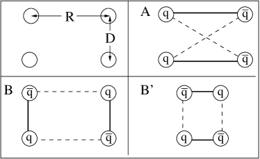
In coordinate space the orientations of the flux tubes depend on the actual distributions of colors and anti-colors. We first discuss the simple case of four particles with colors $cc\bar{c}\bar{c}$ placed on the corners of a rectangle with length $R$ and width $D$ as shown in the upper left part of fig. 5. If all quarks $q$ are lying on the left side and the anti-quarks $\bar{q}$ on the right side the ground state of flux tubes will be like in configuration $A$ in the same figure independent of $R$ and $D$. In this configuration we have two strings of length $R$ with the electric flux pointing in the same direction. In varying $D$ we can examine the interaction energy of two strings of given length $R$ and thus obtain the static string potential for this particular distribution. In Loh et al. (1997a) the potential between two $q\bar{q}$-strings was deduced with a dynamical setup, albeit with the oversimplifying assumption, that the electric fields of two strings add coherently, thus neglecting the intrinsic four-particle interactions.

If in contrast the positions of a quark and an anti-quark are interchanged, there exist two different possibilities. As the energy of a single $q\bar{q}$-string is a monotonically rising function of separation $R$ Quigg and Rosner (1979); Bali et al. (1997); Martens et al. (2004), the lowest four-particle energy is obtained by minimizing the total string length. Consequently if $R>D$, the flux tubes point upside down as in configuration $B$ in fig. 5, whereas, if $R<D$, the flux tubes point from left to right as in configuration $B^{\prime}$. In the CDM the ground state of the flux tubes is found within the model itself by solving the e.o.m. (3), without further input. If one increases $D$ with fixed $R$, the strings will flip from configuration $B$ to $B^{\prime}$ when $D=R$, and one can study the string flip interaction energy. In addition, a dynamical string flip can lead to the dissociation of a $J/\psi$ and thus to $J/\psi$ suppression in relativistic heavy ion collisions Loh et al. (1997b).

We define the interaction between two strings as the difference between the 4-particle energy $E_{4}$ and the sum of the energies $E_{s_{1}}+E_{s_{2}}$ of two independent strings $s_{1}$ and $s_{2}$ with minimal energy. In the case of four particles $q_{1}q_{2}\bar{q}_{1}\bar{q}_{2}$ we calculate the sum of the energies $E_{q_{1}\bar{q}_{1}}$ and $E_{q_{2}\bar{q}_{2}}$ of the strings ($q_{1}\bar{q}_{1}$) and ($q_{2}\bar{q}_{2}$) separately and compare it to the sum of the energies $E_{q_{1}\bar{q}_{2}}$ and $E_{q_{2}\bar{q}_{1}}$ of the competing pairs ($q_{1}\bar{q}_{2}$) and ($q_{2}\bar{q}_{1}$). In the absence of any interactions, the lower value defines the ground state energy of the strings $s_{1}$ and $s_{2}$ (solid lines in fig. 5), the higher an excited state (dashed lines in fig. 5). As the energy of a $q\bar{q}$-string rises monotonously, we do not have to solve the equation of motion for both configurations but only for that with the minimal total string length. The interaction potential $V_{4}$ is then given by

$$V_{4} = E_{4}-(E_{s_{1}}+E_{s_{2}})\quad,$$ (21a)

$$E_{s_{1}}+E_{s_{2}} = \min\left\{\begin{array}[]{ll}E_{q_{1}\bar{q}_{1}}+E_{q_{2}\bar{q}_{2}}\\ E_{q_{1}\bar{q}_{2}}+E_{q_{2}\bar{q}_{1}}\quad.\end{array}\right.$$ (21d)

To illustrate, how the two strings of the ground state influence each other we can define the spatial distribution of the interaction energy $v_{4}$ as:

$$v_{4}(\vec{r})=\varepsilon_{4}(\vec{r})-(\varepsilon_{s_{1}}(\vec{r})+\varepsilon_{s_{2}}(\vec{r}))\quad,$$ (22)

where the energy densities $\varepsilon$ are given as the integrands of Eqs. (4b)- (4d). One comment about the special configuration where the particles are located on the corners of a square is needed. If the two strings are of type $B$/$B^{\prime}$ in fig. 5, both configurations are degenerate for $R=D$, that is the sums of energies $E_{q_{1}\bar{q}_{1}}+E_{q_{2}\bar{q}_{2}}$ and $E_{q_{1}\bar{q}_{2}}+E_{q_{2}\bar{q}_{1}}$ are equal. In that case we calculate the interaction energy density as

$$v_{4}(\vec{r}) = \varepsilon_{4}(\vec{r})-\frac{1}{2}\big{[}(\varepsilon_{q_{1}\bar{q}_{1}}(\vec{r})+\varepsilon_{q_{2}\bar{q}_{2}}(\vec{r}))$$ (23)

$$\hphantom{\varepsilon_{4}(\vec{r})-}+(\varepsilon_{q_{1}\bar{q}_{2}}(\vec{r})+\varepsilon_{q_{2}\bar{q}_{1}}(\vec{r}))\big{]}\quad,$$

i.e. we compare the four-particle density with an incoherent superposition of the 2-string configurations $B$ and $B^{\prime}$. Of course this matters only in the description of the energy density and not of the potential energy $V_{4}$.

Given the exponential behavior of the strings far away from the string axis (cf. Eqs. (19) and (20)), one might estimate the interaction between two separated strings in the following way: Assume both strings point along the x-axis with their axes shifted by $\pm D/2$ away from the string axis. For sufficiently large $D$, the approximations made in section III are valid and the equation for the confinement field is linearized as in Eq. (18). The confinement field of the two string configurations at $|y|\ll D$ then simply is a linear superposition of two single strings, i.e.

$$\chi(y) = \chi_{1}(y)+\chi_{2}(y)\quad\text{with}$$ (24a)

$$\chi_{1/2} = \frac{\chi_{0}}{\sqrt{m_{g}(\frac{D}{2}\pm y)}}e^{\mp m_{g}(y\pm D/2)}\quad,$$ (24b)

with $\chi_{0}$ some constant. As the screening length $\lambda$ of the electric field is substantially smaller than that of the confinement field, $\lambda<\xi$, the electric fields do not contribute much to the total energy density $\varepsilon$, which consequently is dominated by the scalar potential $U(\chi)\approx{\textstyle\frac{1}{2}}m_{g}^{2}\chi^{2}$. The distribution of the interaction energy $v_{4}$ (see Eq. (22)) can be expressed with Eq. (24) as

$$v_{4}(y) = {\textstyle\frac{1}{2}}m_{g}^{2}\left(\chi^{2}(y)-\chi_{1}^{2}(y)-\chi_{2}^{2}(y)\right)$$

$$\approx 2m_{g}^{2}\chi_{0}^{2}\;\frac{e^{-m_{g}D}}{m_{g}D}$$

$$\approx v_{0}\frac{e^{-m_{g}D}}{m_{g}D}\quad,$$ (25)

with $v_{0}$ some constant and where we have used $|y|\ll D$. The strings at a distance $D$ therefore interact with a Yukawa potential, which will be verified numerically later on.

IV.1 Electric field $\vec{D}$

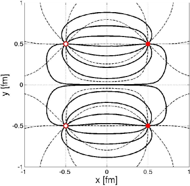
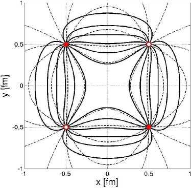
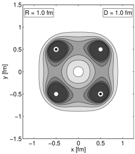
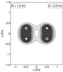
We start our numerical analysis by discussing the electric field lines of two 4-particle configurations with square symmetry in fig. 6, where the particles are located at the corners of a square ($R=D=1\,$fm). In this and the following figures we have a planar particle configuration, although the calculations are done in three dimension. The figures show a cut along the plane $z=0$ of the particles. If not stated otherwise, the calculations for the next figures were done using parameter set PS1 from table 2. In the upper panel, the strings are parallel to each other (type $A$ of fig. 5) and in the lower panel, the strings are anti-parallel to each other (type $B$/$B^{\prime}$ in fig. 5). In both figures the field lines are shown both for the case $\kappa(\vec{r})=\text{const}=1$, i.e. for the color fields obeying the ordinary electromagnetic Maxwell equations (dashed lines), and for $\kappa[\sigma(\vec{r})]$ as calculated from Eqs. (3) (solid lines). All field lines are chosen to start on a circle around each quark (filled dots) with equal angular separation and consequently end on the anti-quarks (open dots). For both orientations the field lines in the CDM calculations are compressed into well defined flux tubes stretching from quarks to anti-quarks, as opposed to the $\kappa=1$ case, where the field lines extend in all directions. The flux tubes of the anti-parallel configuration (lower panel) split symmetrically into two parts connecting each quark with both anti-quarks. Therefore we have a superposition of the two 2-string configurations $B$ and $B^{\prime}$ of fig. 5. Due to the symmetry of the configuration, there is no electric field at all in the center at $\vec{r}=0$.

Figure 6: The electric displacement $\vec{D}$ for $\kappa=\kappa(\sigma)$ (solid lines) and for $\kappa=1$ (dashed lines). The strings have a length $R=1\,\text{fm}$ and their distance is $D=1\,\text{fm}$. The upper and the lower plot show a parallel and an anti-parallel orientation, respectively. The confinement mechanism of the CDM pushes the field lines into well defined flux tubes. For the anti-parallel case the electric flux is distributed symmetrical into types $B$ and $B^{\prime}$.

IV.2 Energy distribution

To analyze the validity of our assumptions in Eqs. (24) and (25) we show the relative difference $\Delta\chi=[\chi-(\chi_{1}+\chi_{2})]/\chi$ (see Eq. (24)) for a configuration of two 1 fm long parallel strings in fig. 7. As expected, the difference approaches 0 for increasing $D$, i.e. the scalar field in the center between two strings is a linear superposition of two isolated strings for sufficiently large $D$. Note, that $\Delta\chi$ becomes concentrated at $|y|\ll D$ for large $D$, i.e. the fields of the strings cancel each other at the centers of each string.

Figure 7: The difference $\Delta\chi=[\chi-(\chi_{1}+\chi_{2})]/\chi$ (cf. Eq. (24)) for a type A configuration of two parallel strings of length $R=1\,\text{fm}$. The plot shows a cut along the $y$-axis transverse to the string axes through the center of the configuration.

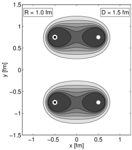
We expect that two strings of given length, that are asymptotically far apart from each other ($D\gg R$), do only weakly interact. If they approach gradually ($D\approx R$), parts of the flux tubes overlap and both the scalar confinement field as well as the electric fields are distorted from their asymptotic shapes. We show the energy densities $\varepsilon(\vec{r})$ of these distorted fields in fig. 8. We choose a string length $R=1\,$fm. In the upper panel, the two strings are parallel to each other (type A) and in the lower panel they are anti-parallel aligned (type $B$/$B^{\prime}$). From left to right the string distance $D$ decreases from $D=1.5\,$fm to $D=0.5\,$fm. The symbols for the quarks are the white dots, those for the anti-quarks the black and white dots. The contour lines are equidistant in energy density in the range $\varepsilon=(0.4\text{GeV/fm}^{3}\ldots 2.4\text{GeV/fm}^{3})$ in steps of $\Delta\varepsilon=0.4\text{GeV/fm}^{3}$.

For large separations ($D=1.5\,\text{fm}>R$) there are two nearly unperturbed strings independent of the orientation of the strings. In this case the string configurations $A$ and $B^{\prime}$ are indistinguishable. Only if the flux tubes get in contact with each other ($D=1\,\text{fm}=R$), the two orientations behave differently. For the parallel case, one finds only a slight attraction between the flux tubes showing up in the distortion towards the center of the two strings. Also the energy density in the center of each string is lowered a little bit.

However, for the case of anti-parallel strings, the flux splits up in the two directions and is the same superposition of types $B$ and $B^{\prime}$ as already seen in fig. 6.

Figure 8: Energy density of two $R=1\,\text{fm}$ long $q\bar{q}$-strings for different distances $D$. The orientation of the strings is parallel (upper panel) and anti-parallel (lower panel). Contour lines are chosen at the values $\varepsilon=(0.4\,\text{GeV/fm}^{3}\ldots 2.4\,\text{GeV/fm}^{3})$ in steps of $\Delta\varepsilon=0.4\,\text{GeV/fm}^{3}$. The darker the area the larger is $\varepsilon$. Quarks are depicted as white dots, anti-quarks as black and white dots. Dark shaded areas are due to the strong Coulomb fields at the particle positions and the contouring is left out here for better visibility of the flux structure.

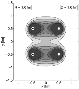
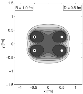
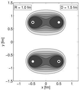
We note, that this reorientation of the flux tubes is found just by solving the equations of motion (3). No external input such as the orientation of a Dirac-string as in the dual color superconductor model Kodama et al. (1997) is needed. The CDM therefore incorporates the feature of string flip as used in the string-flip model Lenz et al. (1986); Voss et al. (1989); Horowitz and Piekarewicz (1991); Boyce and Watson (1994). For the situation of anti-parallel strings, the string flip is not a discontinuous process but a smooth transition. For large separations ($D=1.5\,\text{fm}$), there is already a small part of the energy flux that stretches to the transverse direction. The same is true for $D=0.5\,\text{fm}$ with interchanged roles of types $B$ and $B^{\prime}$. The 4-particle flux tube network is therefore a superposition of types $B$ and $B^{\prime}$ with continuously varying relative strength.

If the two strings approach even further ($D=0.5\,\text{fm}<R$) the two parallel flux tubes melt into an extended flux tube and form a single bag (fig. 8, upper right panel). We observe the contact of the two pairs of likewise charged particles which will lead to a repulsive Coulomb interaction. For the anti-parallel situation however, the string-flip from type $B^{\prime}$ to $B$ has nearly completed and the flux tubes point upside down (fig. 8, lower right panel). The flux tube pattern now shows two flux tubes of length $D<R$. Because of this, the definition of the strings is somewhat ambiguous. We start in varying the distance $D$ between two $R=1\,\text{fm}$ long $q\bar{q}$-strings and finally end up with two $q\bar{q}$-strings of length $D$. Note that in this whole section we denote with the string length the particle distance that we keep fixed, if not stated otherwise explicitly.

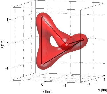
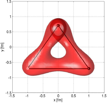
Of course, four particles do not have to be in a plane necessarily. As our numerical realization does all calculations in three dimensions we can easily describe flux tubes stemming from any arbitrary 3-dimensional particle configuration. As one example we show the flux tubes of four particles placed on the corners of a tetrahedron with pairwise distance $R=2\,\text{fm}$. We choose this large particle separation to clearly show the resulting flux tube network. In the 3-dimensional illustration in fig. 9 the equipotential surface of the dielectric function $\kappa=0.3$ is shown. In the center of a $q\bar{q}$-string $\kappa\approx 0.8$ for both parameter sets given in tab. 2 (see Martens et al. (2004)). Therefore the value $\kappa=0.3$ is characterizing the surface of the flux tube. The figure displays two different views of the same configuration, the first a perspective view of the system and the second a projection along the z-axis. Quarks and anti-quarks are marked as black and white spheres, respectively. The four lines are the shortest links between each quark/anti-quark pair. In this highly symmetrical configuration again the flux of each quark is split up into two equal parts pointing towards both anti-quarks, resulting in four equal flux tubes. The centers of the flux tubes are bent slightly towards the center of the configuration, as already seen before in the planar configuration. Moving one $q\bar{q}$-string out of this symmetric configuration would cause two of the four flux tubes to break in favor of the other two. The string flip is therefore seen in the 3-dimensional configurations as well.

Figure 9: (color online). Four particles on the corners of a tetrahedron. All pairwise distances are equal to $R=2\,\text{fm}$. Shown is the equipotential surface $\kappa(\vec{r})=0.3$. Quarks and anti-quarks are marked as dark and light spheres, respectively. The lines are the direct links between each quark/anti-quark pair and are given to show the distortion of the interacting flux tubes. The upper and the lower plot give different views of the same configuration.

IV.3 Interaction potentials

The energy of a $q\bar{q}$-system scales with the particle distance $R$ according to the Cornell-potential given in Eq. (15). In the previous section we have shown the energy distribution of two such interacting strings as well as the difference of the 4-particle state to the incoherent superposition of two equivalent $q\bar{q}$-strings. From the integral of the energy density we get the total energy $E_{4}$ in Eq. (4) and from the corresponding difference of energies in Eq. (21) we extract the interaction potential $V_{4}$. For the following calculation we keep the individual string length $R$ and the relative orientation fixed, and vary only the distance $D$ between the string centers.

The total energy $E_{4}$ of two $R=1\,\text{fm}$ long flux tubes is shown in fig. 10. The orientation is parallel in the upper panel and anti-parallel in the lower panel. The total energy (solid line) is separated in the different energy parts according to Eq. (4). Here we have subtracted from the total energy the energy $E_{\infty}$ of two infinitely separated $q\bar{q}$-strings. In the parallel case this is identical to the potential $V_{4}$, as there is no string flip. For clarity we have separated the curves for the three energy fractions by equal offsets of $0.1\,\text{GeV}$ (upper panel) and $0.5\,\text{GeV}$ (lower panel), respectively.

The total energy saturates for distances $D>1.5\,\text{fm}$, i.e. the strings cease to interact. If they approach each other, we find for the parallel strings a stable distance at $D\approx 0.4\,\text{fm}$. For smaller distances the two likewise charged particles experience the Coulomb repulsion, which is seen only in the electric part of the energy (dashed line). The volume part of the energy (dashed-dotted line) exhibits a small maximum when the two flux tubes get in contact. When they approach each other, the tails of the strings overlap and the two-string configuration takes on a larger effective volume than two isolated strings. As a consequence, the volume energy rises while the electric energy drops down.

For the anti-parallel strings the energy behaves similar for $D\apprge 1\,\text{fm}$. However, for smaller distances the string flip takes place and the energy behaves nearly as two flux tubes that shrink with $D$.

Figure 10: Energy $E_{4}$ of two parallel $q\bar{q}$-strings (top) and two anti-parallel $q\bar{q}$-strings (bottom) with length $R=1\,\text{fm}$. The total energy (solid line) is split into the different energy parts. All energies are reduced by their energies $E_{\infty}$ of two strings asymptotically far apart. The energy parts are separated by constant offsets of $0.1\,\text{GeV}$ (upper panel) and $0.5\,\text{GeV}$ (lower panel) for better visibility.

In fig. 11 we present the interaction potential $V_{4}$ for different string lengths $R$. The orientation is parallel in the upper panel and anti-parallel in the lower panel. The generic form does not change with $R$, but both the position of the minimum and the depth of the potential change with $R$. For the parallel strings the minimum of the potential is moving with increasing $R$ to larger separations $D$. For string lengths $R$ exceeding $1\,\text{fm}$ the location of the minimum basically stays constant. It reaches a stable point at $D\approx 0.4\,\text{fm}$ which is roughly the same size as the radius of the single flux tubes (see tab. 2). Qualitatively this potential resembles the nucleon-nucleon interaction with a short/long range repulsion/attraction and a dip of the order of 100 MeV.

The potential of the anti-parallel strings exhibits a characteristic kink at $D=R$, which is due to the string flip. At this point the orientation of the strings flip from configuration $B$ to $B^{\prime}$. The results obtained in this work differ both qualitatively and quantitatively from that in Loh et al. (1997a). In the older work it was assumed, that the electric fields of the to strings might be added linearly, thus neglecting the 4-body interactions of the color charges. In addition, the parameters chosen there led to flux tubes with a radial width of $\rho_{g}\approx 1\,\text{fm}$, which is much larger than our value $\rho_{g}\approx 0.4\,\text{fm}$ (cf. tab. 2). Consequently, the string interaction in the work of Loh et.al. has a range of about 1 fm. Also there was no stable point in the potential as is seen in our work in fig. 11.

Figure 11: Interaction potential $V_{4}$ of two parallel $q\bar{q}$-strings (top) and two $q\bar{q}$-strings (bottom) with different lengths $R$. The kink in the anti-parallel configuration is due to the string flip at $D=R$.

In fig. 12 we have isolated the potential minimum for different string lengths $R$. In the parallel case (open triangles) the minimum scales linearly with the string length. This can be understood, as for long parallel strings the profile does not change along the flux tube axis. Thus the energy gain per string length should be constant when the two strings get in contact.

For the anti-parallel configuration at $D=R$ but also for the tetrahedron configuration, when all pairwise particle distances are the same, we can parameterize the 4-particle potential in the spirit of the 2-particle Cornell potential $V_{c}(R)$ (15):

$$V_{\square} = 4C_{F}E_{0}-\left(\frac{4}{R}-\frac{2}{\sqrt{2}R}\right)\,C_{F}\alpha+4\tau_{4}\,R-2V_{c}(R)$$ (26a)

$$= -\left(2-\sqrt{2}\right)\,\frac{C_{F}\alpha}{R}+(4\tau_{4}-2\tau)\,R$$

$$V_{\text{tetra}} = 4C_{F}E_{0}-\left(\frac{4}{R}-\frac{2}{R}\right)\,C_{F}\alpha+4\tau_{4}\,R-2V_{c}(R)$$ (26b)

$$= (4\tau_{4}-2\tau)\,R$$

Here the first term in each bracket is due to the four attractive $q\bar{q}$-pairs and the second to the two pairs $qq$ and $\bar{q}\bar{q}$. The constant terms cancel each other exactly. The Coulomb interaction is only partially reduced in the square configuration and completely canceled in the tetrahedron geometry.

In the above parameterization $\tau_{4}$ is an effective 4-particle string tension, whereas $\tau$ denotes the standard $q\bar{q}$-string tension from Eq. (15). Naively one might estimate $\tau_{4}$ in the following way. As we have seen in fig. 8 (lower middle panel) and in fig. 9, the flux tubes of the anti-parallel square configuration and of the tetrahedron configuration do not overlap for string lengths $R>1\,\text{fm}$. The electric flux from each quark is therefore split into two equal flux tubes pointing to the two anti-quarks. It was shown in Martens et al. (2004), that in the CDM the string tension scales with $g_{s}\sqrt{C_{F}}$, i.e. with the charge of the particle. For the two symmetric configurations the 4-particle string tension therefore should be half of the $q\bar{q}$-string tension $\tau_{4}=\tau/2$. In this case the linear confinement terms in Eq. (26a) and Eq. (26b) vanish as well.

In this simplified picture, the potential $V_{\square}$ of the planar anti-parallel configuration should scale Coulomb-like and that for the tetrahedron should vanish very rapidly, compared to the former one. The result of the CDM calculations is shown in fig. 12.

Figure 12: The minimum of the potential $V_{4}(D)$ for different string lengths $R$. The magnitude of the potential $V_{4,\text{min}}$ rises linearly in the parallel case (open triangles) as expected for long homogeneous strings. In the anti-parallel case (solid squares) and the tetrahedron case (solid dots) the attraction gets weaker and shows an unexpected linear increasing behavior.

For both the anti-parallel configuration (solid squares) and the tetrahedron (solid triangles), the potential $V_{4,\text{min}}$ scales linearly with the string length for $R>1\,\text{fm}$. Neither a Coulomb-like nor a rapid cancellation is observed. Thus the 4-particle potential is not a trivial combination of $q\bar{q}$-potentials in the sense of the generalized Cornell potentials as given in Eqs. (26).

The string-string potential was also analyzed in SU(2) lattice theory for anti-parallel configurations in Green et al. (1993). The qualitative behavior of the potential is the same as in our model, although the absolute values of the potential $V_{4}$ are consistently smaller than ours. However, it should be noted that the parameters of our model used in this work are not adjusted to the 4-quark problem, but are fixed to the $q\bar{q}$-properties only. In a very recent SU(3) lattice calculation of the 4-particle system Okiharu et al. (2005a) a multi-Y flux tube picture was proposed, such that the total string length is minimized. This is similar to the Y-like flux tube picture of the 3-quark system. In our model this would be possible with another color content like e.g. $r\bar{r}g\bar{g}$, which is devoted to future work.

Next we turn to the long range behavior of the potential $V_{4}(D)$. From Eqs. (25) we expect a Yukawa potential for sufficiently far separated strings. In fig. 13 we show the negative of the potential $V_{4}$ for different string lengths $R$ in a parallel orientation with parameter set PS1.

Figure 13: Logarithmic plot of the potential $V_{4}(D)$ for different string lengths $R$. The dotted lines are fits of a Yukawa type potential to $V_{4}(D)$. The model parameter correspond to PS1 and the strings are parallel to each other.

The dotted lines are the best fits of a Yukawa type potential $V_{\text{yuk}}(D)=V_{0}\exp\left(-m_{s}D\right)/(m_{s}D)$ as expected from Eq. (25) to the CDM potentials, with $m_{s}$ and $V_{0}$ being fit parameters. For $D\apprge R$ the potential follows nicely the Yukawa behavior. From Eqs. (25) we expect also, that the screening mass $m_{s}$ is given by the curvature $m_{g}$ of the scalar potential $U$ at $\sigma=\sigma_{\text{vac}}$. To test this we show the dependence of $m_{s}$ on $m_{g}$ in fig. 14. From top to bottom, the relative orientation of the strings is parallel, anti-parallel and transverse (tetrahedron like). We have extracted the screening mass from the fit for different string lengths $R$ and for the two parameter sets PS1 and PS2 from tab. 2. The parameter $m_{g}$ takes on the value $m_{g}=1000\,\text{MeV}$ (PS1) and $m_{g}=1500\,\text{MeV}$ (PS2), respectively. The error bars shown in the plot result from variations of the fit interval of $D$ used in the fit. We note, that $V_{4}(D)$ is difficult to extract numerically, as it is an exponentially small difference between to large energies (see Eq. (21)). It should be noted also, that it is numerically more difficult to calculate the potential $V_{4}$ for large string lengths $R$ due to the limited numerical box size but also for parameter set PS2 due to the strongly pronounced maximum of the potential $U$ (see fig. 2). Therefore the error bars are larger for longer strings but also for parameter set PS2. However, within the errors a good agreement of the screening mass to $m_{s}=m_{g}$ is seen. This behavior is almost not dependent on the string length $R$ but also not on the relative orientation.

Figure 14: The screening mass of the interaction potential between two strings for PS1 (solid error bars) and PS2 (dashed error bars). From top to bottom the strings are oriented parallel, anti-parallel and transverse (tetrahedron like) to each other. Within the uncertainties $m_{s}$ is equal to $m_{g}=1000\,\text{MeV}$ (PS1) and $m_{g}=1500\,\text{MeV}$ (PS2).

In the dual Ginzburg-Landau model a Yukawa-type potential was found with a screening mass $m_{s}=1430\,\text{MeV}$ Kodama et al. (1997), which is consistent with our results. Following our above interpretation of $m_{g}$, one might compare these numbers to the glueball mass which has been calculated on the lattice between $1500\,\text{MeV}\leq m_{g}\leq 1700\,\text{MeV}$ Morningstar and Peardon (1997); Michael (1999). Another possibility is to compare $m_{g}$ with the mass $m_{\text{off}}\approx 1200\,\text{MeV}$ of the off-diagonal gluons given on the lattice as well Amemiya and Suganuma (1999). The detailed verification of the Yukawa potential between two strings, as proposed in our description via the CDM, should be a task for future lattice calculations.

V Multi-quark systems

In this section we present CDM results of overall colorless multi-quark systems, with the particle number being larger than four. Such states might in principle exist and a number of possibilities like the pentaquark Diakonov et al. (1997); Nakano et al. (2003), the H-dibaryon Jaffe (1977) and strangelets Farhi and Jaffe (1984); Greiner et al. (1988); Schaffner-Bielich et al. (1997), were eagerly discussed in the literature. Moreover we want to look for a possible transition if the quark number density becomes large as e.g. in the interior of dense neutron stars or in the highly compressed phase in relativistic ion collisions. We study unordered ensembles of quarks and anti-quarks with a varying number of particles. The particles are placed in a given volume which is sufficiently smaller than the numerical box in order to reduce boundary effects.

Figure 15: (color online). Flux tube structure of systems with baryon number $N_{b}>0$ (upper panel) and with vanishing baryon number (lower panel) for different particle densities. We show the equipotential surface of the dielectric function $\kappa_{b}=0.4$ characterizing the surface of the flux tubes. Color codes for the particles are red/green/blue and cyan/magenta/yellow for the quarks and anti-quarks, respectively. The particle numbers for the upper row from left to right are $N=(63,126,255)$ and for the lower row $N=(64,128,256)$ corresponding to particle densities $n=(0.5,1.0,2.0)\,\text{fm}^{-3}$.

The color of the particles are chosen according to two different schemes. In the first we first pick a color $c\in\{r,g,b\}$. This color is assigned to a quark $q$ and simultaneously the corresponding anti-color $\bar{c}$ is assigned to an anti-quark $\bar{q}$. This $q\bar{q}$-pair is thrown randomly into the volume. We repeat this procedure until a given number $N_{m}$ of $q\bar{q}$-states is reached. In this way we get a system with vanishing net baryon number, although baryonic and anti-baryonic clusters might be formed. In the second scheme, we assign the three colors $r,g,b$ to three quarks only and throw them into the volume until a given number $N_{b}$ of baryonic $qqq$ states is reached. In this scheme the baryon number is $N_{b}>0$. Finally we vary the total number of quarks $N=2N_{m}$ and $N=3N_{b}$, respectively, to study the behavior of the quark system for different particle densities $n=N/V$. For each particle density $n$ we choose many different spatial configurations to calculate average quantities as the energy per particle and the bag volume per particle. For this rather qualitative analysis we restrict ourselves to the parameter set PS1. For percolation studies, such as the quark density dependence of the mean bag size, or the formation of a single super cluster, we would need more statistics. This analysis is devoted to future work.

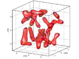
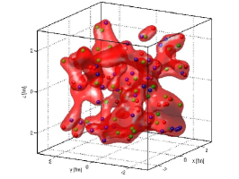
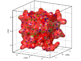
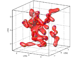
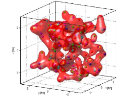
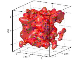
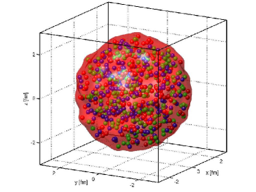
In fig. 15 we show the resulting flux tube structures for the baryonic (upper panel) and the mesonic case (lower panel), respectively. In the latter one one can find all possible color neutral subsystems, namely $q\bar{q}$-states, $qqq$-states and $\bar{q}\bar{q}\bar{q}$ as well as subsystems with larger numbers of quarks and anti-quarks. For these figures the particles were thrown into a cubic box with a size $V=(5\,\text{fm})^{3}$. To visualize the flux tubes in three-dimensional space, we show the position of the particles as small spheres and the equipotential surface of the dielectric function at a value $\kappa=\kappa_{b}=0.4$ characterizing the surface of the flux tubes or bags. The number of quarks in the baryonic case (upper panel) in fig. 15 from left to right is $N=63,126,255$ corresponding to particle densities $n=(0.5,1.0,2.0)\,\text{fm}^{-3}$ or baryon densities $n_{b}=n/3=(1.0,2.0,4.0)\times n_{0}$ with $n_{0}=0.17\,\text{fm}^{-3}$ being nuclear matter density. The number of quarks and anti-quarks in the mesonic case (lower panel) from left to right is $N=64,128,256$ leading approximately to the same particle densities as in the baryonic case.

The formation of well defined bags is clearly seen. For small particle numbers the system is dominated by long, nearly linearly shaped flux tubes. In the baryonic ensemble the smallest clusters are $qqq$-states, whereas in the mesonic ensemble the smallest clusters are in principle $q\bar{q}$-states, $qqq$-states and $\bar{q}\bar{q}\bar{q}$-states. For denser systems the average number of particles per bag grows but still distinct isolated bags are formed. Even for the $n=1.0\,\text{fm}^{-3}$ systems (the two centered figures) the flux tube structure is maintained. The individual and still separated forms are very complex objects and can be interpreted as multi-quark excitations of hadronic particles much akin to the old bootstrap picture of higher lying resonance states Hagedorn (1965); Hagedorn and Ranft (1968). The non-perturbative vacuum is replaced by a spaghetti like perturbative vacuum and both vacua still balance each other. In the systems with $n=2.0\,\text{fm}^{-3}$ (the two figures at the right) nearly all particles are gathered in one single but highly deformed bag. The transition from a small particle density with distinct bags and a small number of particles per bag to a large particle density with only one super-cluster and a large number of particles per bag is similar to a percolation transition which was proposed to occur for the quark hadron transition Matsui and Satz (1986); Bauer (1988); Nardi and Satz (1998).

In the following we analyze this interplay between the perturbative and the non-perturbative vacuum more quantitatively. To reduce numerical boundary effects, we reduce the volume, where the particles are thrown in, to a spherical region with volume $V=\frac{4}{3}\pi r^{3}$ and radius $r=2.5\,\text{fm}$. In fig. 16 we show the energy per particle as a function of particle density in a double logarithmic plot. The upper and the lower plot show a baryonic and a mesonic system, respectively. The solid squares are the values for the total energy per particle averaged over many configurations for each density. The error bars denote the statistical standard deviation for the ensembles of configurations. Clearly, the statistical fluctuations of the energy is largest for the smallest densities. For comparison, we show the electric part of the energy (solid triangles) and the equivalent energy per particle $E_{0}/N$ for the pure Maxwell case, i.e. for $\kappa=1$ everywhere (open dots).

Figure 16: The energy per particle $E/N$ according to Eq. (4) as a function of particle density $n$ for a baryonic (top) and a mesonic (bottom) system. Solid squares symbolize the average values at each density with the statistical standard deviations denoted by the error bars. Triangles are the average values of the electric energy only and the open dots the average energy per particle for the Maxwell case ($\kappa=1$). The dashed line is a fit to the average energy per particle.

The fluctuations for the energy per particle are largest for small densities $n$, as the particles get more and more homogeneously distributed in space with growing density. Both the average total energy and the electric energy follow roughly a power law, whereas the free energy $E_{0}/N$ stays constant. We can estimate the scaling of the total energy as follows. The energy of a cluster scales linearly with the size $L$ of the cluster. For a given particle configuration, the clusters form themselves by minimizing the total energy. Each colored quark builds up a flux tube to the nearest oppositely colored anti-quark or sub-cluster. Thus we can estimate the cluster size by the average particle distance of the system, i.e. $L=n^{-1/3}$. The total energy per particle is therefore $E_{\text{tot}}/N\propto n^{-1/3}$. We have fitted the total energy per particle to the ansatz $E_{\text{tot}}/N=cn^{\beta}$ in the range $n\leq 1\,\text{fm}^{-3}$. The result for the fit parameter was $\beta=-0.35$ and $\beta=-0.36$ for the baryonic and the mesonic system, respectively, which is close to the expected result $\beta=-1/3$. The fit to the low density region overshoots slightly the high density results ($n>3\,\text{fm}^{-3}$), indicating that the assumption of isolated long flux tubes is not valid anymore. Instead, for very large densities, the whole volume is filled with particles homogeneously and the non-perturbative phase is pushed out of the volume $V$. The dielectric function is therefore $\kappa\apprle 1$ everywhere inside $V$ and the electric energy should be the same as for the equivalent free case. Indeed, the electric part of the energy (triangles) approaches the free energy (open dots) for densities $n>5\,\text{fm}^{-3}$.

Figure 17: (color online). 654 quarks randomly distributed in a sphere with radius $r=2.5\,\text{fm}$ and volume $V$. The non-perturbative phase ($\sigma=\sigma_{\text{vac}}$) is pushed out of the sphere completely and $V_{\text{pert}}\approx V$. The bag surface is defined by $\kappa=\kappa_{b}=0.4$.

Another interesting quantity is the specific bag volume per particle $v_{\text{pert}}=V_{\text{pert}}/N$. For small $n$ one finds dominantly bags with two or three particles. The size of the bags per particle decrease with the average particle distance, i.e. with increasing $n$, until with still further increasing density the bags start to overlap and melt together. The decrease of the bag volume per particle slows down or might even turn over to an increase with increasing $n$ in the same way as we have seen in the bump of the volume energy for the melting $q\bar{q}$-system in fig. 10. At a critical density $n_{c}$, when the melting of the bags is completed and the non-perturbative phase is pushed out of the volume $V$ completely, the total perturbative volume can not increase anymore and $V_{\text{pert}}=\text{const}=V$ as shown in fig. 17. With further increasing density $v_{\text{pert}}$ decreases as $n^{-1}$. This critical density $n_{c}$ marks the transition to a system of deconfined quarks and anti-quarks.

Figure 18: The specific bag volume per particle for a baryonic (top) and mesonic system (bottom). Squares denote the average specific bag volume for $\kappa_{b}=0.4$ and triangles that for $\kappa_{b}=0.6$. Error bars indicate the standard deviation for the set of different configurations at each density. At $n_{c}\approx 3\,\text{fm}^{-3}$ the melting of the single bags is completed and the quarks are in the deconfined phase.

We measure the total bag volume as that part in space, where $\kappa\geq\kappa_{b}$. To show the dependence of the bag volume on $\kappa_{b}$ we choose the two values $\kappa_{b}=0.4$ and $\kappa_{b}=0.6$, where $\kappa_{b}=0.4$ ($\kappa_{b}=0.6$) is a surface somewhat more in the exterior (interior) of the bag. Therefore the bag volume measured in this way is larger for $\kappa_{b}=0.4$ than for $\kappa_{b}=0.6$. The result is shown in fig. 18 for the baryonic (top) and the mesonic case (bottom) for $\kappa_{b}=0.4$ (squares) and $\kappa_{b}=0.6$ (triangles). Again the error bars indicate the standard deviation of the specific volume for the different measured configurations at each density. The bag volume per particle shows exactly the anticipated result. It decreases with increasing $n$ for small densities. For $0.3\,\text{fm}^{-3}\leq n\leq 3\,\text{fm}^{-3}$ the specific bag volume $v_{\text{pert}}$ develops a plateau for $\kappa_{b}=0.4$ and rises again for $\kappa_{b}=0.6$. We find the critical density $n_{c}$, i.e. the point where $v_{\text{pert}}$ decreases again, at around $n_{c}\approx 3.0\,\text{fm}^{-3}$. This corresponds to a baryon density $n_{b}=n_{c}/3\approx 6n_{0}$, i.e. six times nuclear matter density or a meson density of approximately $n_{m}=n_{c}/2=1.5\,\text{fm}^{-3}$. We note, that even at the highest density $n=10\,\text{fm}^{-3}$ the mean particle distance is much larger than the intrinsic particle size $r_{0}$ of the particles, so that the color charges do not cancel out each other by overlapping.

Figure 19: The balance between the electric and the volume energy for a baryonic (top) and a mesonic system (bottom). The open squares and the solid dots denote the values of every configuration and their average value, respectively. The two energies are the same within 10% for the numerically reasonable range.

It was one of the results of the work in Martens et al. (2004), that the volume energy $E_{\text{vol}}$ and the electric energy $E_{\text{el}}$ of a $q\bar{q}$-string nearly balance each other. This holds for larger particle densities as well until the system reaches the deconfinement transition. In fig. 19 we show the ratio $E_{\text{vol}}/E_{\text{el}}$ as a function of the particle density for a baryonic (top) and a mesonic system (bottom). It is constant within 10% (neglecting the first point with large uncertainties in the mesonic system) for densities $n\apprle 3.0\,\text{fm}^{-3}$ but falls down for higher densities once the system is in the deconfined phase. The bag volume and therefore the volume energy $E_{\text{vol}}$ are maximal but the electric selfenergy associated with the particles increases with the particle density.

Figure 20: Energy density as a function of particle density $n$. Baryonic (squares) and mesonic systems (triangles) are indistinguishable from each other. The energy density is well described by a power law (dashed line) and is a smooth function even across the critical density at $n_{c}=3.0\,\text{fm}^{-3}$. The vertical and horizontal lines mark the uncertainties in the critical particle density and critical energy density, respectively.

Finally we show the total energy density $\varepsilon=E_{\text{tot}}/V$ as a function of the particle density in fig. 20 for both baryonic (squares) and mesonic (triangles) systems. It follows nicely a polynomial behavior (dashed line) over the whole density range. Remarkably, it is indistinguishable for (static) mesons and baryons. At the critical density $n_{c}=3.0\,\text{fm}^{-3}$ it has a value $\varepsilon_{c}=1.2\,\text{GeV}/\text{fm}^{3}$. Due to the uncertainty in the exact value of the critical density $n_{c}$ we give a band for the critical energy density between $1.0\,\text{GeV}/\text{fm}^{3}$ and $1.3\,\text{GeV}/\text{fm}^{3}$. This is in good agreement with the critical energy density found on the lattice Karsch (2004), where it was found to be between $0.5\,\text{GeV}/\text{fm}^{3}$ and $1.0\,\text{GeV}/\text{fm}^{3}$.

We note, that there are basically no differences in figs. 16, 18 and 19 between baryonic and mesonic systems. Apparently all effects are driven by the particle density, no matter which kind of particles (quarks and anti-quarks or only quarks) are studied.

VI Summary and discussion

The description of the interactions of quarks and gluons, both at high temperatures/densities and in vacuum, from first principles is still an open task to solve. The chromodielectric model offers a tool to describe in a transparent way these interactions while including the confinement phenomenon dynamically within the same framework.

Within the chromodielectric model particles group themselves into color neutral bags with the means of color electric flux tubes. In this work we studied the interactions of these flux tubes with each other. We have seen both on the level of the electric fields and on the level of the energy density, that the flux tubes attract each other. Depending on the relative orientation of the strings, the flux tubes either melt gradually together or change the direction of the electric flux via a characteristic string flip. This should also be seen in future lattice SU(3) calculations for many heavy quarks.

The attraction is seen also in the interaction potential between the strings. The depth as well as the range of the interaction changes with the length of the strings. The interaction depth in the order of a few hundred MeV is relatively strong compared to a rather old analysis made in lattice SU(2) calculations but also compared to a similar analysis within the dual color superconductor model. In the case of the string flip situation the potential can not be described by a simple incoherent superposition of flux tubes, but shows a real multi-particle effect. The long range behavior of the potential can be well described by a Yukawa type potential. The exponential decay of the interaction is expressed by a screening mass between the flux tubes which is rather insensitive to the relative orientations of the strings and to their length. The screening mass scales with the mass parameter $m_{g}$ introduced in the scalar self-interaction of the confinement field. It is a future task to check the model continuously against upcoming results performed on the lattice. On the other hand the Yukawa interaction should be tested in detailed future four-quark lattice calculations. Only recently we have become aware of a lattice study about the interaction of four- and five-quark systems Okiharu et al. (2005a); Okiharu et al. (2005b).

In the studies of the multi-particle systems we have explored the structure of the corresponding flux tubes. The non-perturbative phase is pushed out of the system with increasing particle density. Even for large particle densities compared to nuclear matter constituent quark density, the systems show a heterogeneous structure rather than a homogeneous transition. This situation resembles a typical percolation transition from a hadron to a quark gas. At low particle densities the energy scaling with the particle density is characteristic for a system of strings whose energy scales with the size of the strings. By increasing the particle density, the flux tubes or quark bags start to overlap and to melt into each other. The transition region between isolated hadronic objects and a single large super-cluster, where the quarks behave as deconfined particles, is found to be between $n=1\,\text{fm}^{-3}$ and $n=3\,\text{fm}^{-3}$. The critical energy density of the transition to the deconfined phase is given between $\varepsilon=1.0\text{GeV}/\text{fm}^{3}$ and $\varepsilon=1.3\text{GeV}/\text{fm}^{3}$. This transition shall be examined in the future more carefully in a more detailed percolation analysis. There one could measure for example the onset of the super-cluster, or the distribution of the bag size with respect to its volume or to the number of particles belonging to it, all as a function of the particle density.