Weak boson fusion production of
supersymmetric particles at the LHC

Abstract

We present a complete calculation of weak boson fusion production of colorless supersymmetric particles at the LHC, using the new matrix element generator susy–madgraph . The cross sections are small, generally at the attobarn level, with a few notable exceptions which might provide additional supersymmetric parameter measurements. We discuss in detail how to consistently define supersymmetric weak couplings to preserve unitarity of weak gauge boson scattering amplitudes to fermions, and derive sum rules for weak supersymmetric couplings.

I Introduction

The matter content of the highly successful Standard Model of particle physics is generally considered to be fully revealed after the discovery of the top quark in 1994, although the exact mechanism of electroweak symmetry breaking remains undetermined EWSB . The Standard Model description of spontaneous symmetry breaking is minimal, involving only one additional complex scalar doublet. This introduces an unsatisfactory instability in the scalar sector of the theory. A theoretically more attractive scenario is that spacetime respects the maximal extension of the Poincaré symmetry, supersymmetry (SUSY) SUSY . Its minimal version, the MSSM, simultaneously provides solutions to several problems in high energy physics and cosmology: a candidate for weakly-interacting dark matter; possible unification of the gauge couplings at high energies; and stability of the scalar sector which generates electroweak symmetry breaking through renormalization group running.

SUSY must be a broken symmetry at low energy, as we do not see spin partners of the Standard Model particles. As a result, the squarks, sleptons, charginos, neutralinos and gluino of the MSSM must be massive in comparison to their Standard Model counterparts. Experiments such as LEP and Tevatron run2 have put stringent bounds on some of the SUSY partners’ masses. It will fall to the LHC to perform a conclusive SUSY search covering masses all the way to the TeV scale. Real physics will, however, begin only after a potential SUSY discovery: in particular the strongly-interacting squarks and gluinos can be produced in large numbers at the LHC susy_prod ; Prospino , and their decay cascades typically carry kinematical information about a large fraction of the weakly interacting SUSY spectrum cascades ; bryan_spin . This information can be used to narrow down different SUSY breaking mechanisms sfitter ; pmz_unification .

Much MSSM and non-minimal SUSY phenomenology has been performed over the years in preparation for LHC, nearly all of it using relatively simple dominant $2\to 2$ processes at leading order or next-to-leading order susy_prod ; Prospino . Often, these calculations involve a number of approximations, many of which might not be sufficient for practical applications once the collection of data begins catpiss . Examples include: consideration of spin correlations and finite width effects in SUSY particle production and decays; SUSY-electroweak (EW) and Yukawa interferences to some SUSY-QCD processes; exact rather than common squark masses in the t-channel; and additional $2\to 3$ or $2\to 4$ particle production processes, such as the production of additional hard jets in squark and gluino production Plehn:2005cq , or weak boson fusion (WBF) production of colorless SUSY particles, the subject which we address here.

The last topic is particularly interesting, because it may help us to observe sleptons and weak inos at LHC. These particles can be extremely difficult to observe in direct production channels due to small rates and very large backgrounds, and their appearance in squark and gluino cascade decays can depend on the SUSY breaking scenario. WBF is an electroweak process which naturally leads to high-$p_{T}$ but very far forward taggable jets and little central jet activity. It can be used to observe small electroweak signal rates in a region of phase space not very populated by QCD events. This was applied very successfully to heavy WBF-H and intermediate-mass Higgs boson production in the Standard Model WBF-h , as well as weak boson scattering strong-WW , the MSSM Higgs sector Plehn:1999nw , and to multi–doublet Higgs models Alves:2003vp . As a consequence, there has been recent interest in using the same technique for colorless intermediate-mass SUSY pair production, with investigations of a few channels in limited regions of parameter space WBFino ; WBFsf1 ; WBFsf2 . The reported results were often negative, but appeared to hint at some promising regions of parameter space split_susy . Searching for sleptons and weak inos in these channels can provide useful information about the SUSY Lagrangian.

We present a comprehensive calculation of supersymmetric colorless WBF production channels at the LHC, including a broad scan over parameter space. We also discuss some theoretical issues regarding consistency of electroweak gauge couplings and unitarity of weak boson scattering to weak inos, and their relevance for practical calculations at LHC energies.

To compute these production rates we introduce a new, supersymmetric version of the matrix element generator madgraph ii  Maltoni:2002qb , which properly takes into account various physics aspects which are usually approximated in the literature, such as those listed above. It also provides a practical means to include hard jet radiation effects Plehn:2005cq and eventually match to parton shower simulations, as well as to evaluate more complicated production processes in LHC and linear collider phenomenology catpiss . In Sec. II we discuss susy–madgraph and its model assumptions, $2\to 2$ unitarity as a test of its MSSM couplings, requirements for MSSM electroweak couplings to maintain unitarity of weak scattering processes at high energy, and gauge invariance of WBF processes. We give results for LHC WBF pair production of colorless SUSY particle in Sec. III. We present conclusions in Sec. IV and a technical overview of madgraph ii and susy–madgraph in the Appendix.

II SUSY-MadGraph, unitarity and MSSM couplings

The new matrix element generator susy–madgraph is an extension of the Standard Model madgraph ii package with the new feature of Majorana fermions.  The implementation of madgraph ii into the web–based event generator madevent  Maltoni:2002qb is straightforward and has already been used for the calculations published in Ref. Plehn:2005cq . To include the complete MSSM particle spectrum we use a pair of model data files describing the particle content and its interactions. Specifically, we describe the MSSM as the minimal supersymmetric model which conserves $R$-parity, does not contain any $CP$-violating complex phases, and is CKM- and MNS-diagonal. However, those assumptions can be dropped by straightforward changes in the code. We do not assume any particular SUSY breaking scheme, so the MSSM spectrum and couplings can be handed to it by any spectrum generator, regardless of what assumptions go into constructing the spectrum.

II.1 Setup and Tests

The most work–intensive step in extending madgraph ii to include the MSSM is the correct definition of all couplings in terms of the Lagrangian parameters. To implement the MSSM couplings, we work with the conventions of Refs. gunion_haber and Ref. TP_thesis , and cross-check with those of Ref. MSSMnote . Due to the multiple couplings conventions in the literature MSSMnote ; gunion_haber ; Rosiek:1989rs ; Kuroda:1999ks , we employ a large number of numerical checks to ensure their correctness. In addition to a number of numerical comparisons to published SUSY cross sections at $e^{+}e^{-}$ Barger:1999tn and $pp$ colliders Prospino , we also test the MSSM couplings to electroweak bosons by checking unitarity of $2\to 2$ scattering processes at very high energy. This not only serves to ensure that the couplings are correct, but also reveals a general complication in the use of spectrum generator input from the SUSY Les Houches Accord (SLHA) SLHA . SLHA is a standardized format for communicating SUSY Lagrangian and low-energy parameters, from spectrum generators Allanach:2001kg ; Djouadi:2002ze and SUSY particle widths Muhlleitner:2003vg to multi-purpose Monte Carlos and next–to–leading order predictions Prospino . susy–madgraph uses this convention for the SUSY spectrum input. We discuss this complication in subsection II.3. Finally, we check some 500 $\,2\to 2$ cross sections numerically catpiss between susy–madgraph and the multi-purpose event generators whizard whizard and sherpa sherpa .

II.2 General $VV\to\tilde{\chi}\tilde{\chi}$ Unitarity Sum Rules

A powerful analytical and numerical check of couplings which enter the production of two fermions in gauge boson scattering are unitarity sum rules, which describe the scattering process in the limit of large center-of-mass energy $E$. The general process reads:

$$V_{1}(m_{1},\lambda_{1})+V_{2}(m_{2},\lambda_{2})\to F_{1}(M_{1},\sigma_{1})+\bar{F}_{2}(M_{2},\sigma_{2})\;.$$ (1)

The incoming and outgoing particle masses are $m_{1,2}$ and $M_{1,2}$, respectively. The incoming gauge boson polarizations are $\lambda_{1,2}$, and the final-state fermion helicities are $\sigma_{1,2}=L,R$. Four types of Feynman diagrams can contribute to the above process: $t$-channel exchange of a fermion $F_{k}$ of mass $M_{k}$, $u$-channel exchange of a fermion $F_{\ell}$ with mass $M_{\ell}$, annihilation to an $s$-channel vector boson $V$, or to an $s$-channel scalar $S$. The helicity amplitudes for these four diagrams comprise the matrix element ${\cal M}_{\lambda_{1}\lambda_{2}}^{\sigma_{1}\sigma_{2}}$, from which we derive the sum rules.

The amplitude ${\cal M}_{00}^{RR}$ can be written in terms of general couplings $g_{\pm}$. For example, the interactions between two fermions $F_{1},F_{2}$ and a gauge boson $V$ appear in the Lagrangian as ${\cal L}=g_{\alpha}^{F_{1}F_{2}V}\,\overline{F_{1}}\gamma^{\mu}P_{\alpha}F_{2}V_{\mu}$. The left- and right-handed couplings $\alpha=\pm$ correspond to the left- and right-handed projectors $P_{\pm}=(1\pm\gamma_{5})/2$. Similarly, fermion–scalar couplings appear as ${\cal L}=g_{\pm}^{F_{1}F_{2}S}\,\overline{F_{1}}P_{\pm}F_{2}S$, triple–vector–boson couplings as ${\cal L}=-ig^{V_{1}V_{2}V_{3}}\,\left[(\partial_{\mu}V_{1\nu})(V^{\mu}_{2}V^{\nu}_{3}-V^{\nu}_{2}V^{\mu}_{3})+(\partial_{\mu}V_{2\nu})(V^{\mu}_{3}V^{\nu}_{1}-V^{\nu}_{3}V^{\mu}_{1})+(\partial_{\mu}V_{3\nu})(V^{\mu}_{1}V^{\nu}_{2}-V^{\nu}_{1}V^{\mu}_{2})\right]$ and vector-vector-scalar couplings as ${\cal L}=g^{V_{1}V_{2}S_{3}}\,V_{1}^{\mu}V_{2\mu}S$.

We take $\hat{z}$ to be the incoming beam direction and define the outgoing particles to lie in the $\hat{x}-\hat{z}$ plane. The scattering angle $\sin\theta$ describes the fraction of the final state momentum in the $\hat{x}$ direction:

$${\cal M}_{00}^{RR} = \frac{2E}{m_{1}m_{2}}\sum_{F_{k}}\left[-M_{k}g_{+}^{F_{1}F_{k}V_{1}}g_{-}^{F_{k}F_{2}V_{2}}+\left(M_{1}g_{-}^{F_{1}F_{k}V_{1}}g_{-}^{F_{k}F_{2}V_{2}}+M_{2}g_{+}^{F_{1}F_{k}V_{1}}g_{+}^{F_{k}F_{2}V_{2}}\right)\frac{1+\cos\theta}{2}\right]$$ (2)

$$+ \frac{2E}{m_{1}m_{2}}\sum_{F_{\ell}}\left[-M_{\ell}g_{+}^{F_{1}F_{\ell}V_{2}}g_{-}^{F_{\ell}F_{2}V_{1}}+\left(M_{1}g_{-}^{F_{1}F_{\ell}V_{2}}g_{-}^{F_{\ell}F_{2}V_{1}}+M_{2}g_{+}^{F_{1}F_{\ell}V_{2}}g_{+}^{F_{\ell}F_{2}V_{1}}\right)\frac{1-\cos\theta}{2}\right]$$

$$+ \frac{E}{m_{1}m_{2}}\sum_{V_{3}}g^{V_{1}V_{2}V_{3}}\left[\left(M_{1}g_{-}^{F_{1}F_{2}V_{3}^{*}}-M_{2}g_{+}^{F_{1}F_{2}V_{3}^{*}}\right)\frac{m_{1}^{2}-m_{2}^{2}}{m_{3}^{2}}\right]$$

$$+ \frac{E}{m_{1}m_{2}}\sum_{V_{3}}g^{V_{1}V_{2}V_{3}}\left[\left(M_{1}g_{-}^{F_{1}F_{2}V_{3}^{*}}+M_{2}g_{+}^{F_{1}F_{2}V_{3}^{*}}\right)\cos\theta\right]$$

$$+ \frac{E}{m_{1}m_{2}}\sum_{S}g^{V_{1}V_{2}S}g_{-}^{F_{1}F_{2}S^{*}}+\Delta_{00}^{RR}$$

The remainder $\Delta_{00}^{RR}$ represents terms which do not increase with $E$. Each line in Eq. (2) corresponds to one class of diagrams. The vector boson $V_{3}$ may be $\gamma$ or $Z$. We note that the amplitude Eq.(2) and all equations in this section are obtained in the unitary gauge. A scalar field $S$, therefore, represents both the Higgs bosons and the Goldstone bosons. To obtain sum rules in the Feynman gauge, remove all terms proportional to $m^{2}_{1}-m^{2}_{2}$.

From Eq. 2 we can derive two sum rules for $J=0$ and $J=1$:

$$\underline{J=0:}\qquad \sum_{F_{k}}\left[-2M_{k}g_{+}^{F_{1}F_{k}V_{1}}g_{-}^{F_{k}F_{2}V_{2}}+M_{1}g_{-}^{F_{1}F_{k}V_{1}}g_{-}^{F_{k}F_{2}V_{2}}+M_{2}g_{+}^{F_{1}F_{k}V_{1}}g_{+}^{F_{k}F_{2}V_{2}}\right]$$ (3)

$$+ \sum_{F_{\ell}}\left[-2M_{\ell}g_{+}^{F_{1}F_{\ell}V_{2}}g_{-}^{F_{\ell}F_{2}V_{1}}+M_{1}g_{-}^{F_{1}F_{\ell}V_{2}}g_{-}^{F_{\ell}F_{2}V_{1}}+M_{2}g_{+}^{F_{1}F_{\ell}V_{2}}g_{+}^{F_{\ell}F_{2}V_{1}}\right]$$

$$+ \sum_{V_{3}}g^{V_{1}V_{2}V_{3}}\left(M_{1}g_{-}^{F_{1}F_{2}V_{3}^{*}}-M_{2}g_{+}^{F_{1}F_{2}V_{3}^{*}}\right)\frac{m_{1}^{2}-m_{2}^{2}}{m_{3}^{2}}$$

$$+ \sum_{S}g^{V_{1}V_{2}S}g_{-}^{F_{1}F_{2}S^{*}}=0\;,$$

$$\underline{J=1:}\qquad \sum_{F_{k}}\left[M_{1}g_{-}^{F_{1}F_{k}V_{1}}g_{-}^{F_{k}F_{2}V_{2}}+M_{2}g_{+}^{F_{1}F_{k}V_{1}}g_{+}^{F_{k}F_{2}V_{2}}\right]$$ (4)

$$- \sum_{F_{\ell}}\left[M_{1}g_{-}^{F_{1}F_{\ell}V_{2}}g_{-}^{F_{\ell}F_{2}V_{1}}+M_{2}g_{+}^{F_{1}F_{\ell}V_{2}}g_{+}^{F_{\ell}F_{2}V_{1}}\right]$$

$$+ \sum_{V_{3}}\left[\left(M_{1}g_{-}^{F_{1}F_{2}V_{3}^{*}}+M_{2}g_{+}^{F_{1}F_{2}V_{3}^{*}}\right)g^{V_{1}V_{2}V_{3}}\right]=0\;.$$

Similarly, the amplitude ${\cal M}_{00}^{LL}$ is given by

$${\cal M}_{00}^{LL} = \frac{2E}{m_{1}m_{2}}\sum_{F_{k}}\left[M_{k}g_{-}^{F_{1}F_{k}V_{1}}g_{+}^{F_{k}F_{2}V_{2}}-\left(M_{1}g_{+}^{F_{1}F_{k}V_{1}}g_{+}^{F_{k}F_{2}V_{2}}+M_{2}g_{-}^{F_{1}F_{k}V_{1}}g_{-}^{F_{k}F_{2}V_{2}}\right)\frac{1+\cos\theta}{2}\right]$$ (5)

$$+ \frac{2E}{m_{1}m_{2}}\sum_{F_{\ell}}\left[M_{\ell}g_{-}^{F_{1}F_{\ell}V_{2}}g_{+}^{F_{\ell}F_{2}V_{1}}-\left(M_{1}g_{+}^{F_{1}F_{\ell}V_{2}}g_{+}^{F_{\ell}F_{2}V_{1}}+M_{2}g_{-}^{F_{1}F_{\ell}V_{2}}g_{-}^{F_{\ell}F_{2}V_{1}}\right)\frac{1-\cos\theta}{2}\right]$$

$$- \frac{E}{m_{1}m_{2}}\sum_{V_{3}}g^{V_{1}V_{2}V_{3}}\left[\left(M_{1}g_{+}^{F_{1}F_{2}V_{3}^{*}}-M_{2}g_{-}^{F_{1}F_{2}V_{3}^{*}}\right)\frac{m_{1}^{2}-m_{2}^{2}}{m_{3}^{2}}\right]$$

$$- \frac{E}{m_{1}m_{2}}\sum_{V_{3}}g^{V_{1}V_{2}V_{3}}\left[\left(M_{1}g_{+}^{F_{1}F_{2}V_{3}^{*}}+M_{2}g_{-}^{F_{1}F_{2}V_{3}^{*}}\right)\cos\theta\right]$$

$$- \frac{E}{m_{1}m_{2}}\sum_{S}g^{V_{1}V_{2}S}g_{+}^{F_{1}F_{2}S^{*}}+\Delta_{00}^{LL}\;.$$

leading to two more sum rules

$$\underline{J=0:} \sum_{F_{k}}\left[2M_{k}g_{-}^{F_{1}F_{k}V_{1}}g_{+}^{F_{k}F_{2}V_{2}}-M_{1}g_{+}^{F_{1}F_{k}V_{1}}g_{+}^{F_{k}F_{2}V_{2}}-M_{2}g_{-}^{F_{1}F_{k}V_{1}}g_{-}^{F_{k}F_{2}V_{2}}\right]$$ (6)

$$+ \sum_{F_{\ell}}\left[2M_{\ell}g_{-}^{F_{1}F_{\ell}V_{2}}g_{+}^{F_{\ell}F_{2}V_{1}}-M_{1}g_{+}^{F_{1}F_{\ell}V_{2}}g_{+}^{F_{\ell}F_{2}V_{1}}-M_{2}g_{-}^{F_{1}F_{\ell}V_{2}}g_{-}^{F_{\ell}F_{2}V_{1}}\right]$$

$$- \sum_{V_{3}}g^{V_{1}V_{2}V_{3}}\left(M_{1}g_{+}^{F_{1}F_{2}V_{3}^{*}}-M_{2}g_{-}^{F_{1}F_{2}V_{3}^{*}}\right)\frac{m_{1}^{2}-m_{2}^{2}}{m_{3}^{2}}$$

$$- \sum_{S}g^{V_{1}V_{2}S}g_{+}^{F_{1}F_{2}S^{*}}=0\;,$$

$$\underline{J=1:} \sum_{F_{k}}\left[-M_{1}g_{+}^{F_{1}F_{k}V_{1}}g_{+}^{F_{k}F_{2}V_{2}}-M_{2}g_{-}^{F_{1}F_{k}V_{1}}g_{-}^{F_{k}F_{2}V_{2}}\right]$$ (7)

$$+ \sum_{F_{\ell}}\left[M_{1}g_{+}^{F_{1}F_{\ell}V_{2}}g_{+}^{F_{\ell}F_{2}V_{1}}+M_{2}g_{-}^{F_{1}F_{\ell}V_{2}}g_{-}^{F_{\ell}F_{2}V_{1}}\right]$$

$$+ \sum_{V_{3}}\left[\left(-M_{1}g_{+}^{F_{1}F_{2}V_{3}^{*}}-M_{2}g_{-}^{F_{1}F_{2}V_{3}^{*}}\right)g^{V_{1}V_{2}V_{3}}\right]=0\;.$$

The mixed–helicity amplitudes are

$${\cal M}_{00}^{LR} = -\frac{2E^{2}}{m_{1}m_{2}}\sum_{F_{k}}g_{-}^{F_{1}F_{k}V_{1}}g_{-}^{F_{k}F_{2}V_{2}}\sin\theta+\frac{2E^{2}}{m_{1}m_{2}}\sum_{F_{\ell}}g_{-}^{F_{1}F_{\ell}V_{2}}g_{-}^{F_{\ell}F_{2}V_{1}}\sin\theta$$ (8)

$$-\frac{2E^{2}}{m_{1}m_{2}}\sum_{V_{3}}g^{V_{1}V_{2}V_{3}}g_{-}^{F_{1}F_{2}V_{3}^{*}}\sin\theta+\Delta_{00}^{LR}\;,$$

$${\cal M}_{00}^{RL} = -\frac{2E^{2}}{m_{1}m_{2}}\sum_{F_{k}}g_{+}^{F_{1}F_{k}V_{1}}g_{+}^{F_{k}F_{2}V_{2}}~{}\sin\theta+\frac{2E^{2}}{m_{1}m_{2}}\sum_{F_{\ell}}g_{+}^{F_{1}F_{\ell}V_{2}}g_{+}^{F_{\ell}F_{2}V_{1}}\sin\theta$$ (9)

$$-\frac{2E^{2}}{m_{1}m_{2}}\sum_{V_{3}}g^{V_{1}V_{2}V_{3}}g_{+}^{F_{1}F_{2}V_{3}^{*}}\sin\theta+\Delta_{00}^{RL}\;,$$

and lead to two sum rules

$$-\sum_{F_{k}}g_{-}^{F_{1}F_{k}V_{1}}g_{-}^{F_{k}F_{2}V_{2}}+\sum_{F_{\ell}}g_{-}^{F_{1}F_{\ell}V_{2}}g_{-}^{F_{\ell}F_{2}V_{1}}-\sum_{V_{3}}g^{V_{1}V_{2}V_{3}}g_{-}^{F_{1}F_{2}V_{3}^{*}} = 0\;,$$ (10)

$$-\sum_{F_{k}}g_{+}^{F_{1}F_{k}V_{1}}g_{+}^{F_{k}F_{2}V_{2}}+\sum_{F_{\ell}}g_{+}^{F_{1}F_{\ell}V_{2}}g_{+}^{F_{\ell}F_{2}V_{1}}-\sum_{V_{3}}g^{V_{1}V_{2}V_{3}}g_{+}^{F_{1}F_{2}V_{3}^{*}} = 0\;.$$ (11)

We note, however, that the last two sum rules are not independent from the first four. They can be derived from the helicity–diagonal cases in the limits $M_{1,2}=0$.

To illustrate how the sum rules work we give their explicit form for the process $W^{-}Z\to\widetilde{\chi}^{-}_{1}\widetilde{\chi}^{0}_{1}$. The rule for $(R,R)$ and $J=0$ in terms of general couplings is given in Eq. (3). If we assign $V_{1}=W^{-},V_{2}=Z$ and $F_{1}=\widetilde{\chi}^{-}_{1},F_{2}=\widetilde{\chi}^{0}_{1}\,$, we can exchange $t$–channel neutralinos $F_{k}=\widetilde{\chi}^{0}_{k}$ and $u$–channel charginos $F_{\ell}=\widetilde{\chi}^{-}_{\ell}$. The sum over $s$–channel scalars does not appear in this example because the charged Higgs does not couple to the initial–state gauge bosons. The couplings $g_{\pm}$ for this case are given in the appendix. The sum rule we have to numerically check now becomes:

$$\sum_{k}\left[-2m_{\widetilde{\chi}^{0}_{k}}g_{R}^{\widetilde{\chi}^{-}_{1}\widetilde{\chi}^{0}_{k}W}g_{L}^{\widetilde{\chi}^{0}_{k}\widetilde{\chi}^{0}_{1}Z}+m_{\widetilde{\chi}^{-}_{1}}g_{L}^{\widetilde{\chi}^{-}_{1}\widetilde{\chi}^{0}_{k}W}g_{L}^{\widetilde{\chi}^{0}_{k}\widetilde{\chi}^{0}_{1}Z}+m_{\widetilde{\chi}^{0}_{1}}g_{R}^{\widetilde{\chi}^{-}_{1}\widetilde{\chi}^{0}_{k}W}g_{R}^{\widetilde{\chi}^{0}_{k}\widetilde{\chi}^{0}_{1}Z}\right]$$ (12)

$$+ \sum_{\ell}\left[-2m_{\widetilde{\chi}^{-}_{\ell}}g_{R}^{\widetilde{\chi}^{-}_{1}\widetilde{\chi}^{-}_{\ell}Z}g_{L}^{\widetilde{\chi}^{-}_{\ell}\widetilde{\chi}^{0}_{1}W}+m_{\widetilde{\chi}^{-}_{1}}g_{L}^{\widetilde{\chi}^{-}_{1}\widetilde{\chi}^{-}_{\ell}Z}g_{L}^{\widetilde{\chi}^{-}_{\ell}\widetilde{\chi}^{0}_{1}W}+m_{\widetilde{\chi}^{0}_{1}}g_{R}^{\widetilde{\chi}^{-}_{1}\widetilde{\chi}^{-}_{\ell}Z}g_{R}^{\widetilde{\chi}^{-}_{\ell}\widetilde{\chi}^{0}_{1}W}\right]$$

$$+ g^{WZW}\left(m_{\widetilde{\chi}^{-}_{1}}g_{L}^{\widetilde{\chi}^{-}_{1}\widetilde{\chi}^{0}_{k}W}-m_{\widetilde{\chi}^{0}_{1}}g_{R}^{\widetilde{\chi}^{-}_{1}\widetilde{\chi}^{0}_{k}W}\right)\frac{m_{W}^{2}-m_{Z}^{2}}{m_{W}^{2}}=0$$

To verify these susy–madgraph couplings we numerically check the set of sum rules for the processes $W^{+}W^{-}\to\widetilde{\chi}^{+}_{i}\widetilde{\chi}^{-}_{j}$, $W^{-}Z\to\widetilde{\chi}^{-}_{1}\widetilde{\chi}^{0}_{1}$ and $ZZ\to\widetilde{\chi}^{0}_{1}\widetilde{\chi}^{0}_{3}$. The last process also serves as a check for the proper description of neutralinos with negative mass eigenvalue. In that case we can either use a phase to re–rotate the mass matrix onto positive eigenvalues, which means working with a complex mixing matrix, or we can use the negative mass eigenvalue and make use of an analytic continuation of the expression for the matrix element Barger:1999tn . The two approaches are equivalent at leading order and respect the unitarity sum rules.

In addition to these sum rules, we check unitarity numerically for amplitudes produced by susy-madgraph. Our test includes more than 300 ($2\to 2$) scattering processes with the initial states $VV$,$V\gamma$ and $VH_{i}$, where $V=W^{\pm},Z$ and $H_{i}=h,H,A,H^{\pm}$; and the final states $\tilde{\chi}^{0,\pm}_{i}\tilde{\chi}^{0,\pm,\mp}_{j}$, $VH_{i}$, $\gamma H_{i}$, $H_{i}H_{j}$ and $\tilde{f}_{i}\tilde{f}^{*}_{j}$. We vary the center-of-mass energy from threshold to $10^{4}$ TeV, to avoid problems with machine precision. We require that amplitudes at most approach a constant at high energy. Unfortunately, $2\to 2$ unitarity is not sufficient to check triple-Higgs (or any triple-scalar) couplings. Instead, we verify them by comparison with published results higgs_pair .

II.3 Unitarity and the use of SLHA input

Let us consider a ($2\to 2$) scattering process $VV\to\tilde{\chi}_{i}^{0}\tilde{\chi}_{j}^{0},\tilde{\chi}_{i}^{+}\tilde{\chi}_{j}^{-}$, $V=W^{\pm},Z$ at high energy. There is a well-known gauge cancellation between $s$-, $t$- and $u$-channel diagrams, just as in any Standard Model process $VV\to f\bar{f}$. This limits the high-energy behavior of the amplitude to at most approach a constant. For the cancellation to occur, all couplings and masses in the scattering must be exactly related by a consistent set of electroweak parameters, driven by gauge invariance of the Lagrangian. Even the slightest deviation from this condition will result in the amplitude growing as $E$ or $E^{2}$, depending on the process. This provides a powerful test of the neutralino and chargino couplings. However, when we check the high–energy behavior for weak ino combinations using SLHA input from a default SUSY spectrum generator, the test fails. The answer lies in an inconsistent treatment of electroweak parameters between the default assumption of most spectrum generators, and the way collider processes are conventionally calculated.

The neutralino and chargino sector is described by the mass matrices

$$\left(\begin{array}[]{cccc}m_{\tilde{B}}&0&-m_{Z}s_{w}c_{\beta}&\phantom{-}m_{Z}s_{w}s_{\beta}\\ 0&m_{\tilde{W}}&\phantom{-}m_{Z}c_{w}c_{\beta}&-m_{z}c_{w}s_{\beta}\\ -m_{Z}s_{w}c_{\beta}&\phantom{-}m_{Z}c_{w}c_{\beta}&0&-\mu\\ \phantom{-}m_{Z}s_{w}s_{\beta}&-m_{Z}c_{w}s_{\beta}&-\mu&0\end{array}\right)\qquad\left(\begin{array}[]{cc}m_{\tilde{W}}&\sqrt{2}m_{W}s_{\beta}\\ \sqrt{2}m_{W}c_{\beta}&\mu\end{array}\right)$$ (19)

with the bino, wino and higgsino mass parameters on the diagonal and the gaugino–higgsino mixing masses in the off-diagonal elements. The neutralino and chargino mixing matrices which enter the matrix element are computed with a given set of electroweak parameters $m_{W},m_{Z}$ and $s_{w}(=\sin\theta_{w})$. The same weak parameters also enter the matrix element through the Standard Model gauge boson couplings. Both sets must be consistent to assure proper cancellation of the different diagrams at high energy. This is similar to Standard Model top quark pair production, where the final state masses and the Yukawa coupling have to be identical. The reason for the test failure is because the electroweak parameters used for collider calculations are generally taken to be those at the $Z$ pole, while most spectrum generators run the electroweak parameters up to some scale $Q$ to diagonalize the mass matrices, where the default scale $Q$ is often the SUSY scale, ${\cal O}(1)$ TeV. Even though the electroweak parameter differences at these two scales may seem to be quite small, the mismatch violates gauge invariance, i.e. scattering unitarity is not preserved.

Because the renormalization group evolution implemented in spectrum generators predicts $\overline{\rm DR}$ parameters at the TeV scale, our solution to preserve unitarity is simply to extract the electroweak parameters from the neutralino and chargino mass matrices given in the SLHA input. From the form of the mass matrices in Eq. (19), extracting the effective electroweak parameters is straightforward. If these matrices are loop-improved, this approach is equivalent to assuming a (yet to be explored) universality ds_tp and absorbing the loop corrections into the effective electroweak parameters $m_{Z}^{\rm eff},m_{W}^{\rm eff},s_{w}^{\rm eff}$ and $\tan\beta^{\rm eff}$. We fix the overall coupling strength by $G_{F}=1.16639\times 10^{-5}\,{\rm GeV}^{-2}$, and extract $m_{Z}$, $m_{W}$ and $s_{w}^{\rm eff}$ from the mass matrices. If the weak mixing angle is defined in the on-shell scheme, these three parameters will be consistent also at the TeV scale. These effective parameters are obviously not the pole masses or proper $\overline{\rm MS}$ masses. Therefore, we should examine how large an effect running of the electroweak parameters can have on practical calculations at colliders such as the LHC.

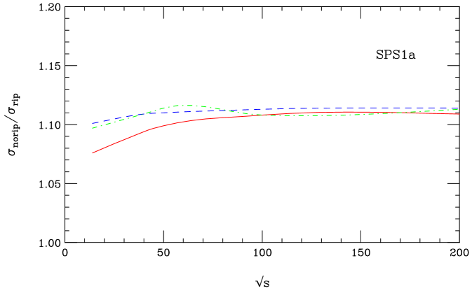
Figure 1: Cross sections with the inconsistent electroweak parameters relative to that with the consistent SLHA ripping scheme described in the text, as function of the hadronic center-of-mass energy. The red (solid) curve is for $\chi^{+}_{1}\chi^{-}_{1}$ pairs, the blue (dashed) curve for $\chi^{+}_{1}\chi^{-}_{1}$ production, and the green (dot-dashed) curve for The cuts of Eqs. (20) and (21) were imposed on the two jets.

We quantify the impact of the different electroweak parameter schemes in Fig. 1, where we show the relative rates of three particular WBF chargino and neutralino production cross sections with and without the SLHA ripping scheme described above. For the SUSY spectrum, we select the generic SPS1a parameter point. At realistic collider energies the technical gauge-invariance violation leads to cross section deviations at a fairly constant level of ${\cal O}(10\%)$ for LHC through VLHC (200 TeV) energies. The flat behavior indicates that we do not yet see unitarity violation numerically at LHC or VLHC energies. Nevertheless, ${\cal O}(10\%)$ corrections from the scheme change exhaust the typical QCD error bars to WBF cross sections Han:1992hr .

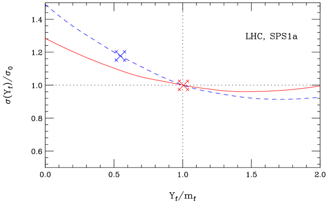
Figure 2: Cross section with varying Yukawa coupling relative to that with $\sigma_{0}(Y_{f}=m_{f})$ for WBF $\tilde{\tau}^{+}_{1}\tilde{\tau}^{-}_{1}$ (red solid) and $\tilde{b}_{1}\tilde{b}^{*}_{1}$ (blue dashed) production. The cuts of Eqs. (20) and (21) are imposed on the two jets. The crosses represent the points where the Yukawa coupling is extracted from the masses and $A_{f}$, as described in the text.

Similar to the above–described problem with electroweak gauge invariance and unitarity, another issue arises in the squark–Higgs and slepton–Higgs couplings. The symmetric scalar mass matrix is completely defined by three entries, usually chosen as two mass eigenvalues and the mixing angle. They can be computed from the left- and right-handed soft–breaking masses, the quark Yukawa coupling, the trilinear mass parameter $A_{q}$ and the Higgs-sector parameters $\mu$ and $\tan\beta$. However, for example in the $\tilde{f}\tilde{f}^{*}h^{0}$ coupling the same parameters $m_{f}$, $A_{f}$, $\mu$, $\tan\beta$ appear in a different combination from the off-diagonal mass matrix entry. If we compute the matrix element for the production process $WW\to\tilde{t}_{i}\tilde{t}_{j}$, these Lagrangian parameters appear in the couplings to an $s$-channel Higgs, but they also enter implicitly through the stop mixing angle (given fixed stop masses). Again, there is potential for a mismatch in the matrix element. In contrast to the electroweak parameter mismatch described above, three-scalar couplings cannot spoil unitarity in $2\to 2$ scattering processes. Although the mismatch breaks SUSY between the top and stop couplings, since the SUSY violation in the three-scalar coupling is soft, this does not reintroduce a quadratic Higgs mass divergence at higher loop order.

There is again a way around this, but it is not as straightforward as in the neutralino/chargino sector. We must choose one SUSY parameter to be extracted from the squark and slepton mass matrices, assuming fixed mass eigenvalues. Because the stau and stop mass matrices are not necessarily evaluated at the same scale, the universal parameters $\tan\beta$ and $\mu$ should not be redefined as effective parameters to cure the mismatch in the stau and stop sectors simultaneously. On the other hand, the renormalization of $A_{f}$ has a strong impact on the perturbative convergence of the light Higgs mass $m_{h}$, while attempting to preserve SUSY by replacing the Yukawa coupling $m_{f}$ as it enters the $\tilde{f}\tilde{f}^{*}h$ coupling also requires a shift in the Yukawa coupling $f\bar{f}h$. Strictly speaking, these couplings are fixed by gauge invariance. However, we also know that, taking Higgs production and decay as an example, calculations using the running $\overline{\rm MS}$ Yukawa couplings significantly improves the perturbative behavior. Given these complications, and given that keeping the mismatch corresponds to only a small shift of a soft–breaking Lagrangian parameter, we use the usual $\overline{\rm DR}$ parameters $m_{f}$, $A_{f}$, $\mu$, $\tan\beta$ in the susy–madgraph couplings $\tilde{f}\tilde{f}\{h,H,A\}$. On the other hand, for practical purposes it will probably be preferable to use the running Yukawa coupling in the $f\bar{f}h$ couping as well as in its $\tilde{f}\tilde{f}^{*}h$ counterpart.

We investigate the practical impact of this inconsistency via the rate change of WBF sfermion pair production (even though the rates are too small to be observed). For stau pairs, the rate change is typically at the per mille level, because of the small tau Yukawa coupling. As another check we construct matrix elements for WBF $\tilde{b}_{1}\tilde{b}^{*}_{1}$ production, even though this is a colored final state. The rate changes for the SPS points vary from negligible (SPS 2,6) to almost a factor of 4 (SPS 4). We show the cross section rates with varying Yukawa coupling relative to those with $Y_{f}=m_{f}$ in Fig. 2 for LHC $\tilde{\tau}^{+}_{1}\tilde{\tau}^{-}_{1}$ and $\tilde{b}_{1}\tilde{b}^{*}_{1}$ production at SPS1a. We see that the Yukawa coupling extracted from the masses and from $A_{f}$ is indeed the expected $\overline{\rm DR}$ or $\overline{\rm MS}$ running mass at the high scale given by the SUSY masses.

II.4 Interplay of WBF and non-WBF processes

As an example, we discuss neutralino pair production, with representative Feynman diagrams shown in Fig. 3. The $WW$-fusion component proceeds via both a $t$–channel diagram involving a mixed gaugino and higgsino $W^{\pm}\widetilde{\chi}^{0}_{i}\widetilde{\chi}^{\mp}_{j}$ coupling, and $s$-channel $Z$ and Higgs boson diagrams mediated via a higgsino-induced $Z\widetilde{\chi}^{0}_{i}\widetilde{\chi}^{0}_{j}$ coupling. The heavy Higgs diagrams essentially do not contribute, as the $HVV$ coupling is proportional to $\cos(\beta-\alpha)$, which vanishes rapidly for large Higgs masses $m_{A}\gtrsim 160$ GeV. The $t$-channel diagrams of the $ZZ$-fusion processes are induced by the higgsino content alone, and have only Higgs bosons in the $s$-channel.

There is a class of bremsstrahlung diagrams where the incoming quarks exchange an electroweak gauge boson, and a quark line emits a $Z$ boson which decays into a neutralino pair: Fig. 3(c). One would naïvely estimate this contribution to be small (after the jet cuts), but there are gauge cancellations between the diagrams which cannot be neglected.

There also exist diagrams where a pair of incoming quarks exchange a gauge boson in the $t$–channel, and one quark line splits to a neutralino and a squark, which decay to neutralino plus quark, Fig. 3(d). In other words, this is a double-bremsstrahlung contribution, induced by the gaugino content of the neutralino. However, for the SPS scenarios, the squarks are heavier than the weak inos, so these diagrams constitute higher-order electroweak resonant neutralino-squark production. Moreover, this contribution does not produce the typical forward jets with central neutralinos, and is a separate gauge set of diagrams. Therefore, we do not include this contribution. Strictly speaking, for production of light neutralinos in scenarios with relatively light squarks (beyond the SPS benchmark points) these diagrams can be non-negligible.

For chargino pair production, the story is much the same, although $s$–channel $Z$ boson diagrams now also have a gaugino component. For slepton/sneutrino production the $WW$ and $ZZ$ fusion diagrams as well as the $Z$-bremsstrahlung are identical to the neutralino case, but the double–bremsstrahlung diagrams do not exist.

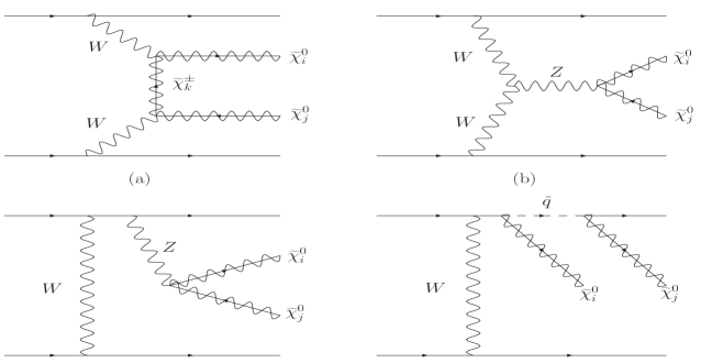
Figure 3: Representative Feynman diagrams for WBF neutralino pair production at a hadron collider: (a) $t$-channel chargino exchange; (b) $s$-channel $Z$ boson (or Higgs bosons, not shown); (c) $Z$ bremsstrahlung; (d) double–neutralino bremsstrahlung, which in most cases is a higher-order electroweak correction to on-shell squark-neutralino production.

As a check of the consistent generation of amplitudes by susy–madgraph , we test the $U(1)_{EM}$ (electromagnetic) gauge invariance of WBF production of MSSM particles. To test electromagnetic gauge invariance, we generate matrix elements for WBF production plus a photon for a number of weak ino and sfermion pairs. These are $(2\to 5)$ processes, which would be impossible to calculate without automated tools such as susy-madgraph. We then set the photon polarization vector numerically to its four-momentum, and simultaneously set all particle widths to zero, to confirm that the matrix element vanishes.

Although we had hoped that the EM gauge invariance of the generated amplitudes with one additional photon emission would demonstrate the need to include non-WBF amplitudes, mainly because the photon is partly an electroweak ($W^{3}$) boson, we found that the WBF and non-WBF amplitudes give rise to separately EM gauge invariant sets in all the processes we studied. It is interesting that there are further $U(1)_{EM}$ gauge-invariant subsets, some of which are the set of all diagrams involving a four-point $VVSS$ coupling – that is, of two gauge bosons and two MSSM scalars – as well as diagrams involving two scalars and $s$-channel Higgs propagators, as they arise from the SUSY Lagrangian $D$-terms, which are separately gauge invariant.

Checking only the $U(1)_{EM}$ gauge-invariance of the WBF processes is, therefore, not a verification that calculations neglecting bremsstrahlung diagrams is gauge invariant with respect to the full electroweak theory. For this one has to check the exact electroweak Ward identities for each process. This is not as simple as replacing the vector boson wave function with its momenta, as it is in the photon case. Unfortunately, testing the full electroweak gauge invariance of WBF processes is beyond the scope of this paper, as it requires further development of automated matrix element tools.

While previous calculations WBFino ; WBFsf1 ; WBFsf2 are therefore $U(1)_{EM}$ gauge-invariant, some of their results are incorrect due to large cancellations between diagram subsets, most notably for slepton-sneutrino production. We quantify this in the next Section.

III Weak boson fusion cross section results

A characteristic of WBF is that the incoming quarks are scattered at relatively small angles, but at typical transverse momentum of order $\sim M_{V}/2$. These scattered partons can easily be identified as jets in CMS cms_tdr and ATLAS atlas_tdr for $p_{T}\gtrsim 20\;{\rm GeV}$. We thus impose generic observability kinematic cuts on the (parton–level) scattered quarks:

$$p_{T}(j)>20\,{\rm GeV}\,,\qquad|\eta(j)|<5.0\;.$$ (20)

Unless the WBF process involves an internal photon propagator, which occurs only for charged particle production, almost all the cross section will pass these cuts. A further characteristic of WBF is that the two jets lie in opposite hemispheres, i.e. far forward and far backward, with large pseudorapidity separation between them. We can therefore impose the typical WBF separation cut

$$|\eta(j_{1})-\eta(j_{2})|>4.2\,,$$ (21)

which corresponds to a pseudorapidity separation of 3 units between the jet cone edges, using a typical LHC jet cones size of radius 0.6. This cut typically suppresses the WBF rate by a factor 3-4. SUSY-QCD backgrounds which include a pair of hard jets can be a few orders of magnitude larger than the WBF cross section before cuts. However, they are typically suppressed by 2-3 orders of magnitude by the WBF cuts. Normally, for a WBF analysis one imposes further constraints to ensure the WBF-produced decay products lie between the two jets, and the two forward jets form a large invariant mass. These cuts usually result in little additional loss of the signal. Because they are not necessary for our illustrative purposes here, we ignore such refinement of the signal rates. Forward-tagged jets are typically identified with these cuts with an efficiency of $\epsilon_{\rm tag}=0.86$, predicted by detector simulation, for low-luminosity running. This number might decrease somewhat for high-luminosity running Gianotti:2002xx .

We use leading-order CTEQ6L1 parton densities Pumplin:2002vw in our calculations, with factorization scale $\mu_{f}=(m_{1}+m_{2})/2$, where $m_{1}$ and $m_{2}$ are the masses of the heavy particle pair produced. The electroweak parameters except for $G_{F}$ are taken from the SLHA model files, as described in the previous section. We investigate all SPS points sps , MSSM parameter space benchmarks designed to represent a number of canonical scenarios to align experimental studies and phenomenology. We consider them to be only starting points for investigation, with no assumption that the scenarios are more likely to be realized in nature than any other.

III.1 Charginos and neutralinos

Neutralinos and charginos can be pair-produced in WBF, for their rates we always impose the tagging jet cuts of Eqs.(20) and (21). Most cross sections are at the attobarn [ab] level, with a few exceptions. Any cross section below 1 fb is almost certainly going to be unobservable, unless it has a large branching ratio to a particularly distinctive final state that can be observed with high detection efficiency, such as multiple electrons or muons. Even then it may have sizable backgrounds from cascade decays of colored SUSY particles produced at QCD strength. We comment on possible noteworthy cases.

We first show the neutralino pair production cross sections in Table 1, which are almost universally at the few-attobarn level. In SPS scenarios, the lightest neutralino is mostly bino, which reduces the coupling to weak bosons, while the higgsinos are heavy. The single exception to tiny neutralino pair cross sections in all SPS scenarios is $\tilde{\chi}^{0}_{2}\tilde{\chi}^{0}_{2}$ production, where the $\tilde{\chi}^{0}_{2}$ is mostly wino with a sizable higgsino fraction. For this case, rates typically range from a tenth of a femtobarn to half a femtobarn. At SPS9, the $\chi^{0}_{2}$ decays mainly to $\ell^{+}\ell^{-}\tilde{\chi}^{0}_{1}(\ell=e,\mu,\tau)$, which results in a sizable detection efficiency of due to the 4-lepton final state with large missing transverse momentum. Since there are very few Standard Model backgrounds which could produce this signature, SUSY backgrounds are the dominant source and likely small. There is some chance this channel could be observed, although with very low statistics unless one considers the LHC luminosity upgrade, SLHC Gianotti:2002xx .

However, as we show in Table 5, the Drell-Yan (DY) rate for $\tilde{\chi}^{0}_{2}\tilde{\chi}^{0}_{2}$ production is far larger Prospino . Unfortunately, the DY and WBF production mechanisms are not very complementary, in the sense that both processes involve the same gaugino–induced coupling to light-flavor quarks and the higgsino–induced coupling to gauge bosons. The similar-size rate for WBF $\tilde{\chi}^{0}_{1}\tilde{\chi}^{0}_{1}$ production at SPS9 is likely uninteresting, as the WBF $Z\to\nu\bar{\nu}$ rate is much larger Eboli:2000ze .

We next show the chargino pair production cross sections in Table 2. For opposite-sign production, where we do not apply the forward tagging jet cuts as the signature is already highly distinctive, they are at most around a femtobarn for $\tilde{\chi}^{+}_{1}\tilde{\chi}^{-}_{1}$ at SPS1a and SPS9. However, given that the WBF $W^{+}W^{-}$ background is several orders of magnitude larger, we do not expect this signal to be observable. Moreover, WBF production of opposite-sign charginos is again much smaller than the direct DY production. Much more interesting are the same–sign chargino rates, also shown in Table 2. While the signal rates stay below a femtobarn even for $\tilde{\chi}^{+}_{1}\tilde{\chi}^{+}_{1}$, the Standard Model WBF $W^{+}W^{+}$ background is now similar in size to the signal. Instead, the main background would more likely come from SUSY cascades, for example from gluino pairs or squark pairs which decay to like–sign dileptons. Those production cross sections are typically above $\sim 100$ pb Prospino , but the branching fractions which lead to dileptons are usually tiny. If like–sign chargino pairs were clearly identifiable at LHC, it would provide conclusive evidence that the neutralinos appearing in the $t$-channel are Majorana fermions, although this would first require separate evidence that the chargino or the neutralino candidates are in fact fermions. We are not aware of any other way of demonstrating this at the LHC, and extraction of this information out of cascade decays would likely be tedious. Of course, a future linear collider operating in $e^{-}e^{-}$ mode would provide definitive proof of the Majorana nature of the neutralinos.

A complete study of signal and backgrounds for same-sign chargino production is on the way. The analysis breaks down into two dominant regions of parameter space for the signal: where the chargino decays predominantly to $W^{\pm}\tilde{\chi}^{0}_{1}$ followed by a leptonic $W$ boson decay; and where it decays preferentially to $\tilde{\tau}^{\pm}\nu_{\tau}$ and the stau ultimately decays to a lepton and the lightest neutralino. In both cases, the $\tilde{\chi}^{0}_{1}$ gives rise to significant missing transverse energy. The final state is then a pair of far-forward/backward high-$p_{T}$ jets, a pair of same-sign central leptons (also expected to be high-$p_{T}$ due to the large mass of the cascade parent), and significant missing transverse energy. There would also be very little additional jet activity, due to the electroweak nature of the scattering process, as mentioned in the Introduction. The efficiency for such a signal would be extremely high. The Standard Model WBF $W^{\pm}W^{\pm}$ background is also of ${\cal O}(1)$ fb strong-WW , but should display markedly different lepton kinematics. SUSY backgrounds would arise primarily from QCD squark and gluino production, which are often collectively at the tens to hundreds of picobarn level. However, only a small fraction of these will give high-$p_{T}$ forward jets from the cascade decay to jets plus charginos, and much of the sample will have additional high-$p_{T}$ jets which can be vetoed. The lepton kinematics will again be significantly different, as the typical relatively light charginos (compared to the squarks and gluinos) will yield much higher-$p_{T}$ leptons.

Finally, we show the mixed chargino-neutralino production cross sections in Tables 3 and 4. These are also at the attobarn level, the only exception being $\chi^{\pm}_{1}\chi^{0}_{2}$ production, with a typical rate of ${\cal O}(1)$ fb. However, this should be compared to the DY rate of many hundreds of femtobarn as shown in Table 5.

SPS	1a0	1b0	20	30	40	50	60	70	80	90
$\chi^{0}_{1}\chi^{0}_{1}$	0.0030	00	00	00	00	0.0010	00	0.0010	00	0.460
$\chi^{0}_{1}\chi^{0}_{2}$	0.0180	0.0010	0.0020	0.0010	0.0040	0.0030	0.0030	0.0080	0.0030	00
$\chi^{0}_{1}\chi^{0}_{3}$	0.0020	00	00	00	0.0010	00	0.0010	0.0030	0.0010	0.0020
$\chi^{0}_{1}\chi^{0}_{4}$	0.0020	00	00	00	0.0010	00	0.0010	0.0010	0.0010	0.0020
$\chi^{0}_{2}\chi^{0}_{2}$	0.520	0.100	0.240	0.100	0.260	0.290	0.0390	0.0570	0.150	00
$\chi^{0}_{2}\chi^{0}_{2}$	0.0490	0.0080	0.0090	0.0080	0.0260	0.0080	0.0090	0.0170	0.0160	00
$\chi^{0}_{2}\chi^{0}_{4}$	0.0650	0.0110	0.0110	0.0110	0.0340	0.0090	0.0230	0.0450	0.0220	00
$\chi^{0}_{3}\chi^{0}_{3}$	0.0060	0.0010	0.0010	0.0010	0.0040	0.0010	0.0040	0.0090	0.0030	00
$\chi^{0}_{3}\chi^{0}_{4}$	0.0080	0.0010	0.0010	0.0010	0.0040	0.0010	0.0050	0.0130	0.0030	00
$\chi^{0}_{4}\chi^{0}_{4}$	0.0070	0.0010	0.0010	0.0010	0.0040	0.0010	0.0080	0.0200	0.0030	00

Table 1: Cross sections [fb] for WBF neutralino pair production at LHC, for all MSSM benchmark SPS points, using the kinematic cuts of Eqs. (20) and (21). Cross sections are shown to two significant digits or rounded to the nearest attobarn, and those smaller than half an attobarn are shown as zero.

SPS	1a0	1b0	20	30	40	50	60	70	80	90
$\chi^{+}_{1}\chi^{-}_{1}$	1.60	0.260	0.630	0.270	0.740	0.770	0.130	0.230	0.420	1.30
$\chi^{+}_{1}\chi^{-}_{2}$	0.0560	0.0100	0.0110	0.0100	0.0290	0.0100	0.0150	0.0280	0.0190	0.0020
$\chi^{+}_{2}\chi^{-}_{2}$	0.0350	0.0070	0.0040	0.0060	0.0200	0.0030	0.0300	0.0680	0.0150	00
$\chi^{+}_{1}\chi^{+}_{1}$	0.930	0.220	0.480	0.230	0.510	0.570	0.0670	0.0770	0.310	0.880
$\chi^{+}_{1}\chi^{+}_{2}$	0.130	0.0220	0.0280	0.0220	0.0700	0.0150	0.0720	0.140	0.0490	0.0020
$\chi^{+}_{2}\chi^{+}_{2}$	0.0010	00	00	00	0.0010	00	0.0110	0.0320	0.0010	00
$\chi^{-}_{1}\chi^{-}_{1}$	0.280	0.0560	0.130	0.0580	0.140	0.160	0.0170	0.0200	0.0830	0.250
$\chi^{-}_{1}\chi^{-}_{2}$	0.0400	0.0060	0.0050	0.0060	0.0210	0.0050	0.0180	0.0360	0.0140	0.0010
$\chi^{-}_{2}\chi^{-}_{2}$	00	00	00	00	00	00	0.0020	0.0070	00	00

Table 2: Cross sections [fb] for WBF opposite-sign and same-sign chargino pair production at LHC, for all MSSM benchmark SPS points, using the kinematic cuts of Eqs. (20) and (21) for opposite-sign charginos only (see text). Cross sections are shown to two significant digits or rounded to the nearest attobarn, and those smaller than half an attobarn are shown as zero.

SPS	1a0	1b0	20	30	40	50	60	70	80	90
$\chi^{+}_{1}\chi^{0}_{1}$	0.0150	0.0010	0.0010	0.0010	0.0040	0.0020	0.0030	0.0100	0.0030	0.530
$\chi^{+}_{1}\chi^{0}_{2}$	0.640	0.100	0.260	0.110	0.300	0.310	0.0440	0.0740	0.170	00
$\chi^{+}_{1}\chi^{0}_{3}$	0.0420	0.0070	0.0070	0.0070	0.0210	0.0070	0.0080	0.0180	0.0130	0.0010
$\chi^{+}_{1}\chi^{0}_{4}$	0.0440	0.0070	0.0080	0.0070	0.0240	0.0060	0.0120	0.0220	0.0150	0.0010
$\chi^{+}_{2}\chi^{0}_{1}$	0.0030	00	00	00	0.0010	00	0.0010	0.0010	0.0010	0.0010
$\chi^{+}_{2}\chi^{0}_{2}$	0.0290	0.0050	0.0050	0.0050	0.0150	0.0040	0.0100	0.0210	0.0100	00
$\chi^{+}_{2}\chi^{0}_{3}$	0.0070	0.0010	0.0010	0.0010	0.0040	0.0010	0.0050	0.0110	0.0030	00
$\chi^{+}_{2}\chi^{0}_{4}$	0.0080	0.0010	0.0010	0.0010	0.0040	0.0010	0.0080	0.0210	0.0030	00

Table 3: Cross sections [fb] for WBF positive-sign chargino plus neutralino pair production at LHC, for all MSSM benchmark SPS points, using the kinematic cuts of Eqs. (20) and (21). Cross sections are shown to two significant digits or rounded to the nearest attobarn, and those smaller than half an attobarn are shown as zero.

SPS	1a0	1b0	20	30	40	50	60	70	80	90
$\chi^{-}_{1}\chi^{0}_{1}$	0.0090	0.0010	0.0010	0.0010	0.0020	0.0010	0.0020	0.0060	0.0020	0.320
$\chi^{-}_{1}\chi^{0}_{2}$	0.390	0.0590	0.150	0.0620	0.180	0.190	0.0260	0.0440	0.0970	00
$\chi^{-}_{1}\chi^{0}_{3}$	0.0270	0.0040	0.0050	0.0040	0.0140	0.0050	0.0060	0.0120	0.0090	0.0010
$\chi^{-}_{1}\chi^{0}_{4}$	0.0270	0.0050	0.0050	0.0040	0.0150	0.0040	0.0070	0.0140	0.0090	0.0010
$\chi^{-}_{2}\chi^{0}_{1}$	0.0020	00	00	00	0.0010	00	00	0.0010	0.0010	0.0010
$\chi^{-}_{2}\chi^{0}_{2}$	0.0180	0.0030	0.0030	0.0030	0.0100	0.0030	0.0060	0.0130	0.0060	00
$\chi^{-}_{2}\chi^{0}_{3}$	0.0040	0.0010	00	0.0010	0.0020	0.0010	0.0030	0.0070	0.0020	00
$\chi^{-}_{2}\chi^{0}_{4}$	0.0050	0.0010	00	0.0010	0.0030	00	0.0050	0.0120	0.0020	00

Table 4: Cross sections [fb] for WBF negative-sign chargino plus neutralino pair production at LHC, for all MSSM benchmark SPS points, using the kinematic cuts of Eqs. (20) and (21). Cross sections are shown to two significant digits or rounded to the nearest attobarn, and those smaller than half an attobarn are shown as zero.

	SPS 1a		SPS8
	0  DY0	WBF0	0  DY0	WBF0
$\chi^{0}_{2}\chi^{0}_{2}$	0025.40	0.520	0002.900	0.150
$\chi^{+}_{1}\chi^{-}_{1}$	7050	1.60	2120	0.420
$\chi^{+}_{1}\chi^{0}_{2}$	8280	0.640	2760	0.170
$\chi^{-}_{1}\chi^{0}_{2}$	4740	1.260	1420	0.310

Table 5: Drell-Yan (DY) and WBF pair production cross sections [fb] for two representative MSSM benchmark SPS points. The DY results were calculated with Prospino2.0 Prospino at NLO.

III.2 Sleptons and sneutrinos

The second type of supersymmetric WBF processes is the production of charged sleptons and sneutrinos, again with the tagging jet cuts of Eqs. (20) and (21). Smuon cross sections are identical to those for selectrons, as their masses are identical, so we omit them in our tables.

Sneutrino pair production rates, shown in Table 6, are at the attobarn level and universally too small to be observed. The charged slepton cross sections and the mixed cases (cf. Tables 7 and 8) show similarly limited promise (in contradiction with Refs. WBFsf1 ; WBFsf2 ). At least part of this discrepancy is due to large cancellations between the pure-WBF diagrams and bremsstrahlung, where the incoming quarks scatter off each other via a weak boson, and the sparticle pair arises from $Z/W$-Bremsstrahlung off a quark line. The cancellation is practically nil for the neutral current ($ZZ$ fusion) in slepton pair production, as well as sneutrino pairs, but a little more than a factor 3 in the charged current ($WW$ fusion), which dominates, leaving an overall cancellation of about a factor 3. The cancellation is much larger for mixed sneutrino-slepton pairs, about a factor 30. Refs. WBFsf1 ; WBFsf2 considered only the WBF diagrams and so did not notice the cancellations. We emphasize that these cancellations reflect electroweak gauge invariance, which we discussed previously.

A useful comparison is to note that the Drell-Yan rates for selectron and stau pairs, shown in Table 9, are in the few tens of fb range for many SPS points. One might have hoped to use just the WBF sneutrino pair signals, which would often give missing energy plus forward-tagged jet signals, but because of the ultra-low signal rates, this will again be swamped by WBF $Z\to\nu\bar{\nu}$ boson production Eboli:2000ze .

SPS	1a0	1b0	20	30	40	50	60	70	80	90
$\tilde{\nu}_{e}\tilde{\nu}^{*}_{e}$	000.0280	000.0040	00	000.0070	0.0010	000.0110	000.0030	000.0110	000.0030	0.0020
$\tilde{\nu}_{\tau}\tilde{\nu}^{*}_{\tau}$	000.0270	000.0040	00	000.0070	0.0020	000.0110	000.0030	000.0110	000.0030	0.0020

Table 6: Cross sections [fb] for WBF sneutrino pair production at LHC, for all MSSM benchmark SPS points. Cross sections are shown to two significant digits or rounded to the nearest attobarn, and those smaller than half an attobarn are shown as zero.

SPS	1a0	1b0	20	30	40	50	60	70	80	90
$\tilde{e}_{L}^{+}\tilde{e}_{L}^{-}$	0.0520	0.0080	00	0.0140	0.0030	0.0220	0.0060	0.0220	0.0070	0.0040
$\tilde{e}_{R}^{+}\tilde{e}_{R}^{-}$	0.0450	0.0060	00	0.0210	0.0010	0.0170	0.0080	0.0690	0.0230	0.0010
$\tilde{\tau}_{1}^{+}\tilde{\tau}_{1}^{-}$	0.0530	0.0160	00	0.0230	0.0060	0.0190	0.0080	0.0750	0.0250	0.0020
$\tilde{\tau}_{1}^{+}\tilde{\tau}_{2}^{-}$	0.0070	0.0030	00	0.0010	0.0010	0.0020	00	0.0020	00	0.0010
$\tilde{\tau}_{2}^{+}\tilde{\tau}_{2}^{-}$	0.0430	0.0060	00	0.0140	0.0030	0.0200	0.0060	0.0210	0.0060	0.0020

Table 7: Cross sections [fb] for WBF charged slepton pair production at LHC, for all MSSM benchmark SPS points. Cross sections are shown to two significant digits or rounded to the nearest attobarn, and those smaller than half an attobarn are shown as zero.

SPS	1a0	1b0	20	30	40	50	60	70	80	90
$\tilde{e}_{L}^{+}\tilde{\nu}_{e}$	0.0260	0.0030	00	0.0060	0.0010	0.0100	0.0020	0.0100	0.0030	0.0020
$\tilde{\tau}_{1}^{+}\tilde{\nu}_{\tau}$	0.0050	0.0030	00	0.0010	0.0010	0.0010	00	0.0020	00	0.0010
$\tilde{\tau}_{2}^{+}\tilde{\nu}_{\tau}$	0.0230	0.0030	00	0.0060	0.0010	0.0090	0.0020	0.0100	0.0030	0.0010

Table 8: Cross sections [fb] for WBF charged slepton plus sneutrino pair production at LHC, for all MSSM benchmark SPS points. Cross sections are shown to two significant digits or rounded to the nearest attobarn, and those smaller than half an attobarn are shown as zero. We neglect showing the charge-conjugate processes as the cross sections are trivially small.

	SPS 1a		SPS8
process	0  DY0	WBF0	0  DY0	WBF0
$\tilde{e}_{L}^{+}\tilde{e}_{L}^{-}$	22.50	0.0520	002.490	0.0070
$\tilde{e}_{R}^{+}\tilde{e}_{R}^{-}$	29.00	0.0450	14.30	0.0230
$\tilde{\tau}_{1}^{+}\tilde{\tau}_{1}^{-}$	34.40	0.0530	16.00	0.0250
$\tilde{\tau}_{2}^{+}\tilde{\tau}_{2}^{-}$	18.30	0.0430	002.400	0.0060

Table 9: Cross sections [fb] for Drell-Yan (DY) v. WBF slepton pair production at LHC, for two representative MSSM benchmark SPS points. Cross sections are shown to two significant digits or rounded to the nearest attobarn, and those smaller than half an attobarn are shown as zero. The DY results were calculated with Prospino Prospino at NLO.

IV Conclusions

We have presented a thorough investigation of weak boson fusion production of colorless SUSY particles at the LHC. We find the cross sections to be almost universally unobservably small for all SPS scenarios, usually at the few-attobarn level, especially in the case of sleptons and sneutrinos. The smallness of the cross sections is partly due to large cancellations which take place at the amplitude level between WBF-type diagrams and bremsstrahlung diagrams.

There remain two or three exceptions, where the rates are potentially interesting: $\tilde{\chi}^{0}_{2}\tilde{\chi}^{0}_{2}$ production, which would give a highly distinctive four-lepton final state in many MSSM scenarios; and same-sign chargino production $\tilde{\chi}^{\pm}_{i}\tilde{\chi}^{\pm}_{i}$. The latter case is especially intriguing, because it can constitute definitive proof already at LHC that the neutralinos in the $t$-channel are Majorana fermions. This is a crucial test for a candidate SUSY discovery. It might also provide information on the relative hierarchy of the wino and higgsino mass parameters. We sketched how such an analysis would proceed, identifying the dominant final state channels as a function of MSSM parameterization and outlining the major relevant backgrounds.

To perform these calculations, we developed the matrix element generator susy–madgraph which includes the complete MSSM with $R$-parity and without additional $CP$ violation, and does not assume any particular SUSY breaking scheme. It relies on the input from any SUSY spectrum generator in the SLHA format. We tested the MSSM implementation by comparing with the literature for all known $2\to 2$ collider scattering processes, and additionally via unitarity of scattering amplitudes at high energy and $U(1)_{EM}$ gauge invariance. We furthermore derived analytical sum rules for neutralino and chargino electroweak gauge couplings from unitarity in all modes of $VV\to\tilde{\chi}\tilde{\chi}$ scattering.

We identified an issue of electroweak gauge invariance using SLHA input during development, on account of the unitarity checks: the default output of SUSY spectrum generators, combined with the default use of electroweak parameters for collider calculations, forms an inconsistent set of electroweak parameters. This misalignment can lead to sizable deviations in physical cross sections, relative to the known level of QCD perturbative uncertainty in the overall rates. susy–madgraph uses electroweak parameters taken from the neutralino and chargino mixing matrices to form a consistent set.

Appendix A MadGraph II technical details

madgraph  Stelzer:1994ta is a package which generates matrix elements for a user-input scattering process at a specified order in $\alpha_{s}$ and $\alpha$. The Fortran output it provides calls the helas Murayama:1992gi library of helicity amplitude subroutines, which can calculate any possible dimension-4 Lagrangian term. It is extremely versatile, allowing as many external particles as one has computing power to handle, and allowing the user to require certain intermediate states while restricting others. It maintains all helicity correlations throughout.

The original version had the Standard Model explicitly incorporated into the Fortran code. To facilitate additions beyond the Standard Model such as SUSY, madgraph was rewritten such that it could read model information from an input file, and also handle Majorana fermions. These new features are incorporated into the release of madgraph ii , designed to work with madevent  Maltoni:2002qb , and briefly described below. The new version also now provides sub-amplitudes in leading-$N_{c}$ color flows that allow it to be interfaced to standard parton-shower Monte Carlo programs such as pythia pythia , herwig herwig or sherpa sherpa .

The existence of Majorana fermions in SUSY required another significant modification to the code. madgraph ’s use of helas requires a well-defined continuous fermion flow for the calculation of amplitudes and their proper interference. This continuous flow is not automatically satisfied by processes that involve Majorana fermions. Therefore, for a given process madgraph ii defines a continuous fermion flow Denner:1992me , chosen randomly from the two possible direction for any fermion line. For every fermion, madgraph also defines a charge conjugate fermion with the opposite flow. Using this complete set of fermions, and requiring continuity of the fictitious fermion flow, madgraph ii is able to generate all of the appropriate diagrams, with the proper interference structure. In this scheme, conflicting fermion flows (“clashing arrows”) are avoided by choosing a fermion flow randomly from the two possible directions, charge-conjugating the external wavefunction on one end of the fermion flow to match the chosen direction, and calculating the charge-conjugated vertex at the point of clashing arrows.

The Standard Model Lagrangian in madgraph ii is specified in two files, defining the particle content and the dimension-4 interactions, respectively. The user must set the defined couplings in a separate Fortran routine, with values to be passed to the matrix elements by common block. The first file, particles.dat, defines all particles in the model. The next few lines show the format of the space-delineated file.

d       d~        F        S      ZERO  ZERO    T   d    1
t       t~        F        S      TMASS TWIDTH  T   t    6
e-      e+        F        S      ZERO  ZERO    S   e    11
g       g         V        C      ZERO  ZERO    O   _    21
w-      w+        V        W      WMASS WWIDTH  S   W    -24
h       h         S        D      HMASS HWIDTH  S   h    25
p uu~dd~ss~cc~g

The first two entries define the characters to be used for the particle and antiparticle respectively. Notice in the case of a gluon it is the same symbol. The third entry gives the spin of the particle, choices are F for spin 1/2 fermions, V for spin 1 vectors and S for spin 0 scalars. The fourth entry defines the type of line in the Feynman diagram, SCWD correspond to solid, curly, wavy, and dashed respectively. The next two entries are text strings representing the particles mass and width. The seventh entry gives the color information, valid options are STO, representing color singlet, triplet or octet. The eighth entry is the text to be displayed on the Feynman diagram labeling the line, and the last entry is a number representing the particles ID to be used in interfacing with the QCD Les Houches Accord. In this format the complete set of Standard Model particles can be specified with just 17 lines.

At the LHC it is particularly useful to generate a set of subprocesses by summing over groups of particles, e.g. partons in the proton, or final–state jets. The last line above defines the symbol p to represent the sum over the light quarks and gluon. There can not be any spaces between the particles that are to be summed over.

The second file necessary to define a model is interactions.dat. As the name implies this file contains information about the allowed interactions. madgraph ii currently allows for 3- and 4-particle vertices to be implemented using the space-delimited format shown below.

d d g GG QCD
g g g G  QCD
g g g g G G QCD QCD
d d a  GAD QED
d u w- GWF QED
u d w+ GWF QED

The first line shows the vertex for a $d\bar{d}g$ QCD interaction. The first three entries are the particles appearing at the dimension-4 vertex. The ordering convention for fermion-fermion-boson interactions is first the incoming fermion, followed by the outgoing fermion, and the outgoing boson last. This is also illustrated in the interactions of the $W^{+}$ and $W^{-}$. The fourth entry contains the coupling strength for the interaction as it appears in the Fortran file, and the last entry specifies the type of coupling. This final string can be used to limit the diagrams to a certain order if $\alpha$ or $\alpha_{s}$. The four–gluon vertex illustrates a four-particle interaction. The first four entries define the particles involved in the interaction, the product of the fifth and sixth entries gives the couplings for the interaction, and the last two entries specify the couplings involved.

This is all the information required to define an interaction. The color structure of the vertex is inferred based on the color of the particles, and the Lorentz structure is inferred based on their spins. This format is compact, and the complete Standard Model (using diagonal CKM and MNS matrices) is specified with only 58 lines.

susy–madgraph is the madgraph ii package with two data files (as described above) which completely specify the MSSM Lagrangian. Moreover, it includes a Fortran routine which reads in the MSSM parameters from an SLHA files, and another which calculates the MSSM couplings. The input file may be generated by any MSSM spectrum generator. If one wants to include particle decays in the matrix elements, their widths must be specified in the SLHA file, and are read in automatically by the code. The couplings are assumed to conserve $CP$, but are written in the include file in such a way as to facilitate later inclusion of $CP$-violation, if the user chooses to add it. Chargino and neutralino mixing matrices are defined to be real. Negative neutralino masses appearing in the propagators do not introduce any errors for the Majorana scheme we implemented.

Appendix B Neutralino and Chargino Feynman Rules

In this appendix we give the explicit Feynman rules and couplings needed to evaluate the example sum rule for the process $W^{-}Z\to\widetilde{\chi}^{-}_{1}\widetilde{\chi}^{0}_{1}$ given as an example at the end of Section II.2. Unfortunately, there are (at least) two sets of conventions for the chargino and neutralino mixing matrices present in the literature, namely Refs. gunion_haber ; TP_thesis and Ref. MSSMnote . We give all formulas in both conventions.

B.1 Neutralino and Chargino Mixing

The chargino mass matrix according to Ref. MSSMnote reads

$$M_{C} = \left(\begin{array}[]{cc}M_{2}&\sqrt{2}m_{W}c_{\beta}\\ &\\ \sqrt{2}m_{W}s_{\beta}&\mu\end{array}\right).$$ (25)

and can be diagonalized using two unitary matrices ${U^{C}_{R}}^{\dagger}M_{C}U^{C}_{L}={\rm diag}(m_{\widetilde{\chi}^{-}_{j}})$.

The unitary mixing matrices $U^{C}_{L,R}$ can be expressed in terms of two mixing angles. As long as these mixing matrices are real, one of the mass eigenvalues can in principle be negative. In that case a phase can be introduced in one of the mixing matrices (e.g. $U^{C}_{R}$), or (as long as $CP$ is conserved) we can perform the matrix element calculation with negative mass eigenvalues, simply by analytically continuing the expressions for the matrix element. Note that in helaswe have to provide positive mass values for the spinor calculations. The analytic continuation holds only for the matrix element.

The chargino mixing matrices can easily be translated into the conventions used in Refs. gunion_haber ; TP_thesis , with the chargino mixing matrix Eq. (19). In that case we use the unitary matrices $U$ and $V$ to diagonalize the transpose of the chargino mixing matrix defined in Eq. (25) $U^{*}{\cal M}_{C}^{T}V^{-1}$. The translation rule becomes:

$$U_{L}^{C}=U^{\dagger}\;,\qquad\qquad U_{R}^{C}=V^{T}\;.$$ (26)

The neutralino mass matrix in both sets of conventions is identical, so we just copy the expression from Eq. (19):

$$M_{N} = \left(\begin{array}[]{cccc}M_{\tilde{B}}&0&-m_{Z}s_{w}c_{\beta}&m_{Z}s_{w}s_{\beta}\\ 0&M_{\tilde{W}}&m_{Z}c_{w}c_{\beta}&-m_{Z}c_{w}s_{\beta}\\ -m_{Z}s_{w}c_{\beta}&m_{Z}c_{w}c_{\beta}&0&-\mu\\ m_{Z}s_{w}s_{\beta}&-m_{Z}c_{w}s_{\beta}&-\mu&0\\ \end{array}\right)\;.$$ (31)

It is diagonalized as ${U^{N}_{R}}^{\dagger}M_{N}U^{N}_{L}={\rm diag}(m_{\widetilde{\chi}^{0}_{j}})\,$. Because the neutralinos are Majorana fermions, the mass matrix $M_{N}$ is symmetric. Hence, up to a matrix of phase factors $P$, two unitary matrices $U^{N}_{L}$ and $U^{N}_{R}$ can be chosen as $U^{N}_{L}=U_{N}P^{*}$ and $U^{N}_{R}=U_{N}^{*}P$. Again, if $CP$ is conserved and we are willing to work with negative neutralino mass eigenvalues using analytic continuation of the matrix element expression, we can choose $P=1$. Alternatively, we can absorb the phase of the mass eigenvalue into a then-complex mixing matrix.

Again, we can translate the neutralino mixing matrices in the conventions of Refs. gunion_haber ; TP_thesis . There, the mass matrix in the bino–wino basis is diagonalized by a unitary transformation $N^{*}{\cal M}_{N}N^{-1}$. The mixing matrices are now related by:

$$U_{L}^{N}\equiv U^{N}=N^{\dagger}\;,\qquad\qquad U_{R}^{N}=(U_{L}^{N})^{*}=N^{T}\;.$$ (32)

B.2 Couplings for interactions with gauge bosons

Using the above definitions, we write out the couplings of gauge bosons to neutralinos and charginos for both set of conventions defined above. The symbol $U$ without any superscript refers to the chargino mixing matrix according to Refs. gunion_haber ; TP_thesis . Note that the fermion order in helasand in the sum rules is $g_{L,R}^{f_{\rm out}f_{\rm in}V}$, while in the susy–madgraph file interactions.dat it is $g_{R,L}^{f_{\rm in}f_{\rm out}V}$, where $f_{\rm in,out}$ are not necessarily both particle (as opposed to antiparticle). Instead, they are the particle or antiparticle for the rule as read directly off a Feynman diagram of the interaction vertex. This is important to remember in constructing chargino rules for susy–madgraph . The mixed chargino–neutralino–$W$ couplings are:

$$g_{L}^{\widetilde{\chi}^{0}_{i}\widetilde{\chi}^{-}_{j}W} = \left(g_{L}^{\widetilde{\chi}^{-}_{j}\widetilde{\chi}^{0}_{i}W}\right)^{*}=-g\left[\left(U^{N}_{L}\right)_{2i}^{*}\left(U^{C}_{L}\right)_{1j}+\frac{1}{\sqrt{2}}\left(U^{N}_{L}\right)_{3i}^{*}\left(U^{C}_{L}\right)_{2j}\right]$$

$$\phantom{\left(g_{R}^{\widetilde{\chi}^{-}_{j}\widetilde{\chi}^{0}_{i}W}\right)^{*}}=-g\left[N_{i2}\;U_{j1}+\frac{1}{\sqrt{2}}N_{i3}\;U_{j2}\right]\;,$$

$$g_{R}^{\widetilde{\chi}^{0}_{i}\widetilde{\chi}^{-}_{j}W} = \left(g_{R}^{\widetilde{\chi}^{-}_{j}\widetilde{\chi}^{0}_{i}W}\right)^{*}=-g\left[\left(U^{N}_{R}\right)_{2i}^{*}\left(U^{C}_{R}\right)_{1j}-\frac{1}{\sqrt{2}}\left(U^{N}_{R}\right)_{4i}^{*}\left(U^{C}_{R}\right)_{2j}\right]$$

$$\phantom{\left(g_{L}^{\widetilde{\chi}^{-}_{j}\widetilde{\chi}^{0}_{i}W}\right)^{*}}=-g\left[N_{i2}^{*}\;V_{j1}-\frac{1}{\sqrt{2}}N_{i4}^{*}\;V_{j2}\right]\;.$$

All neutralino and chargino mixing matrices are defined above and $g$ is the usual weak gauge coupling. The chargino couplings to a photon or a $Z$ boson are proportional to the gauge couplings $g_{Z}=g/c_{w}$, with the usual weak mixing angle $c_{w}=\cos\theta_{w}$ and $s_{w}=\sin\theta_{w}$:

$$g_{L}^{\widetilde{\chi}^{-}_{i}\widetilde{\chi}^{-}_{j}Z} = g_{Z}\left[\left(U^{C}_{L}\right)^{*}_{1i}\left(U^{C}_{L}\right)_{1j}+\frac{1}{2}\left(U^{C}_{L}\right)^{*}_{2i}\left(U^{C}_{L}\right)_{2j}-s_{w}^{2}\delta_{ij}\right]$$

$$= g_{Z}\left[U^{*}_{i1}\;U_{j1}+\frac{1}{2}U^{*}_{i2}\;U_{j2}-s_{w}^{2}\delta_{ij}\right]\;,$$

$$g_{R}^{\widetilde{\chi}^{-}_{i}\widetilde{\chi}^{-}_{j}Z} = g_{Z}\left[\left(U^{C}_{R}\right)^{*}_{1i}\left(U^{C}_{R}\right)_{1j}+\frac{1}{2}\left(U^{C}_{R}\right)^{*}_{2i}\left(U^{C}_{R}\right)_{2j}-s_{w}^{2}\delta_{ij}\right]$$

$$= g_{Z}\left[V^{*}_{i1}\;V_{j1}+\frac{1}{2}V^{*}_{i2}\;V_{j2}-s_{w}^{2}\delta_{ij}\right]\;,$$

$$g^{\widetilde{\chi}^{-}_{i}\widetilde{\chi}^{-}_{i}A}_{L} = g^{\widetilde{\chi}^{-}_{i}\widetilde{\chi}^{-}_{i}A}_{R}=e\;.$$ (37)

Finally, the neutralino coupling to the $Z$ is:

$$g_{L}^{\widetilde{\chi}^{0}_{i}\widetilde{\chi}^{0}_{j}Z} = -\frac{1}{4}g_{Z}\left[\left(U^{N}_{L}\right)^{*}_{3i}\left(U^{N}_{L}\right)_{3j}-\left(U^{N}_{L}\right)^{*}_{4i}\left(U^{N}_{L}\right)_{4j}\right]\;,$$ (38)

$$= -\frac{1}{4}g_{Z}\left[N_{i3}\;N^{*}_{j3}-N_{i4}\;N^{*}_{j4}\right]\;,$$

$$g_{R}^{\widetilde{\chi}^{0}_{i}\widetilde{\chi}^{0}_{j}Z} = -g_{L}^{\widetilde{\chi}^{0}_{j}\widetilde{\chi}^{0}_{i}Z}\;.$$ (39)

Due to the Majorana nature of the neutralinos, the indices $i,j$ should be taken as $i<j$, and there is an additional factor of 2 for $i=j$ in Eqs. (38) and (39). For the sum rules in Feynman gauge we need the Goldstone couplings to $W,Z$, neutralinos and charginos:

$$g^{W^{-}Z\omega^{+}}=-g^{W^{+}Z\omega^{-}}=-ig_{Z}m_{W}s_{w}^{2}$$ (40)

$$g_{L}^{\widetilde{\chi}^{0}_{i}\widetilde{\chi}^{-}_{j}\omega^{+}} = \left(g_{R}^{\widetilde{\chi}^{-}_{j}\widetilde{\chi}^{0}_{i}\omega^{+}}\right)^{*}$$

$$= -\frac{\displaystyle i}{\sqrt{\displaystyle 2}}g\left[\left(U^{N}_{R}\right)^{*}_{2i}\left(U^{C}_{L}\right)_{2j}-\sqrt{2}\left(U^{N}_{R}\right)^{*}_{3i}\left(U^{C}_{L}\right)_{1j}+\frac{\displaystyle s_{w}}{\displaystyle c_{w}}\left(U^{N}_{R}\right)^{*}_{1i}\left(U^{C}_{L}\right)_{2j}\right]c_{\beta}$$

$$= -\frac{\displaystyle i}{\sqrt{\displaystyle 2}}g\left[N^{*}_{i2}U_{j2}-\sqrt{2}N^{*}_{i3}U_{j1}+\frac{\displaystyle s_{w}}{\displaystyle c_{w}}N^{*}_{i1}U_{j2}\right]c_{\beta}$$

$$g_{R}^{\widetilde{\chi}^{0}_{i}\widetilde{\chi}^{-}_{j}\omega^{+}} = \left(g_{L}^{\widetilde{\chi}^{-}_{j}\widetilde{\chi}^{0}_{i}\omega^{+}}\right)^{*}$$

$$= -\frac{\displaystyle i}{\displaystyle\sqrt{2}}g\left[\left(U^{N}_{R}\right)_{2i}\left(U^{C}_{R}\right)_{2j}+\sqrt{2}\left(U^{N}_{L}\right)^{*}_{4i}\left(U^{C}_{R}\right)_{1j}+\frac{\displaystyle s_{w}}{\displaystyle c_{w}}\left(U^{N}_{R}\right)_{1i}\left(U^{C}_{R}\right)_{2j}\right]s_{\beta}$$

$$= -\frac{\displaystyle i}{\displaystyle\sqrt{2}}g\left[N_{i2}V_{j2}+\sqrt{2}N^{*}_{i4}V_{j1}+\frac{\displaystyle s_{w}}{\displaystyle c_{w}}N_{i1}V_{j2}\right]s_{\beta}$$

References

-
(1)
For reviews see:
W. Kilian,
Electroweak Symmetry Breaking,
Springer 2005;
A. Djouadi, arXiv:hep-ph/0503172 and arXiv:hep-ph/0503173. -
(2)
For reviews of supersymmetry, see:
S. P. Martin,
arXiv:hep-ph/9709356;
I. J. R. Aitchison, arXiv:hep-ph/0505105. - (3) http://www-cdf.fnal.gov/physics/exotic/exotic.html; http://www-d0.fnal.gov/public/new/new_public.html.
- (4) S. Dawson, E. Eichten and C. Quigg, Phys. Rev. D 31, 1581 (1985).
-
(5)
W. Beenakker, R. Höpker, M. Spira and P. M. Zerwas,
Nucl. Phys. B 492, 51 (1997);
W. Beenakker, M. Krämer, T. Plehn, M. Spira and P. M. Zerwas, Nucl. Phys. B 515, 3 (1998);
W. Beenakker et al., Phys. Rev. Lett. 83, 3780 (1999) -
(6)
H. Bachacou, I. Hinchliffe and F. E. Paige,
Phys. Rev. D 62, 015009 (2000);
B. C. Allanach, C. G. Lester, M. A. Parker and B. R. Webber, JHEP 0009, 004 (2000);
B. K. Gjelsten, D. J. Miller and P. Osland, JHEP 0412, 003 (2004);
B. K. Gjelsten, D. J. Miller and P. Osland, JHEP 0506, 015 (2005);
D. J. Miller, P. Osland and A. R. Raklev, arXiv:hep-ph/0510356. -
(7)
A. J. Barr,
Phys. Lett. B 596, 205 (2004);
J. M. Smillie and B. R. Webber, JHEP 0510, 069 (2005);
A. J. Barr, arXiv:hep-ph/0511115. -
(8)
R. Lafaye, T. Plehn and D. Zerwas,
arXiv:hep-ph/0404282;
P. Bechtle, K. Desch and P. Wienemann, arXiv:hep-ph/0412012. - (9) G. A. Blair, W. Porod and P. M. Zerwas, Phys. Rev. D 63, 017703 (2001)
- (10) K. Hagiwara, F. Krauss, T. Plehn, D. Rainwater, J. Reuter, S. Schumann, and W. Kilian [CATPISS collaboration] arXiv:hep-ph/0512260; for a collection of reference processes see: http://141.30.17.245/hep/hep/pages/external/susy_comparison.html
- (11) T. Plehn, D. Rainwater and P. Skands, arXiv:hep-ph/0510144.
-
(12)
R. N. Cahn, S. D. Ellis, R. Kleiss and W. J. Stirling,
Phys. Rev. D 35, 1626 (1987);
V. D. Barger, T. Han and R. J. N. Phillips, Phys. Rev. D 37, 2005 (1988);
R. Kleiss and W. J. Stirling, Phys. Lett. B 200, 193 (1988);
D. Froideveaux, in Proceedings of the ECFA Large Hadron Collider Workshop, Aachen, Germany, 1990, ed. G. Jarlskog and D. Rein (CERN report 90-10, 1990), Vol II, p. 444;
M. H. Seymour, ibid, p. 557;
U. Baur and E.W.N. Glover, Nucl. Phys. B 347, 12 (1990) and Phys. Lett. B 252, 683 (1990);
V. Barger, K. Cheung, T. Han, J. Ohnemus and D. Zeppenfeld, Phys. Rev. D 44, 1426 (1991). -
(13)
D. Rainwater and D. Zeppenfeld,
JHEP 9712, 005 (1997) and
Phys. Rev. D 60, 113004 (1999)
[Erratum-ibid. D 61, 099901 (2000)];
D. Rainwater, D. Zeppenfeld and K. Hagiwara, Phys. Rev. D 59, 014037 (1999);
T. Plehn, D. Rainwater and D. Zeppenfeld, Phys. Rev. D 61, 093005 (2000)
and Phys. Rev. Lett. 88, 051801 (2002);
N. Kauer, T. Plehn, D. Rainwater and D. Zeppenfeld, Phys. Lett. B 503, 113 (2001);
T. Plehn and D. Rainwater, Phys. Lett. B 520, 108 (2001). -
(14)
V. D. Barger, K. Cheung, T. Han and R. J. N. Phillips,
Phys. Rev. D 42, 3052 (1990);
D. A. Dicus, J. F. Gunion and R. Vega, Phys. Lett. B 258, 475 (1991);
D. A. Dicus, J. F. Gunion, L. H. Orr and R. Vega, Nucl. Phys. B 377, 31 (1992). - (15) T. Plehn, D. L. Rainwater and D. Zeppenfeld, Phys. Lett. B 454, 297 (1999).
- (16) A. Alves, O. Eboli, T. Plehn and D. L. Rainwater, Phys. Rev. D 69, 075005 (2004).
-
(17)
A. Datta, P. Konar and B. Mukhopadhyaya,
Phys. Rev. D 65, 055008 (2002);
A. Datta, P. Konar and B. Mukhopadhyaya, Phys. Rev. Lett. 88, 181802 (2002). - (18) A. Datta and K. Huitu, Phys. Rev. D 67, 115006 (2003).
-
(19)
D. Choudhury et al., Phys. Rev. D 68, 075007 (2003);
P. Konar and B. Mukhopadhyaya, Phys. Rev. D 70, 115011 (2004). -
(20)
see e.g. :
W. Kilian, T. Plehn, P. Richardson and E. Schmidt,
Eur. Phys. J. C 39, 229 (2005);
K. Cheung and J. Song, Phys. Rev. D 72, 055019 (2005). - (21) F. Maltoni and T. Stelzer, JHEP 0302, 027 (2003).
- (22) J. F. Gunion and H. E. Haber, Nucl. Phys. B 272, 1 (1986) [Erratum-ibid. B 402, 567 (1993)].
- (23) T. Plehn, arXiv:hep-ph/9809319.
- (24) G.-C. Cho and K. Hagiwara, unpublished.
- (25) J. Rosiek, Phys. Rev. D 41, 3464 (1990) [Erratum-hep-ph/9511250].
- (26) M. Kuroda, arXiv:hep-ph/9902340.
- (27) V. D. Barger, T. Han, T. J. Li and T. Plehn, Phys. Lett. B 475, 342 (2000).
- (28) B. Allanach, P. Skands et al., JHEP 0407, 036 (2003); T. Hahn, arXiv:hep-ph/0408283; J. A. Aguilar-Saavedra et al., to appear in Eur.Phys.J. C, [arXiv:hep-ph/0511344].
- (29) B. C. Allanach, Comput. Phys. Commun. 143, 305 (2002).
- (30) A. Djouadi, J. L. Kneur and G. Moultaka, arXiv:hep-ph/0211331.
- (31) M. Mühlleitner, A. Djouadi and Y. Mambrini, arXiv:hep-ph/0311167.
- (32) W. Kilian, T. Ohl and J. Reuter, http://www-ttp.physik.uni-karlsruhe.de/whizard
- (33) T. Gleisberg, S. Höche, F. Krauss, A. Schälicke, S. Schumann and J. C. Winter, JHEP 0402, 056 (2004).
-
(34)
T. Plehn, M. Spira and P. M. Zerwas,
Nucl. Phys. B 479, 46 (1996)
[Erratum-ibid. B 531, 655 (1998)];
A. Krause, T. Plehn, M. Spira and P. M. Zerwas, Nucl. Phys. B 519, 85 (1998). - (35) T. Fritzsche, T. Plehn and D. Stöckinger, in preparation.
- (36) T. Han, G. Valencia and S. Willenbrock, Phys. Rev. Lett. 69, 3274 (1992).
- (37) CMS TP, report CERN/LHCC/94-38 (1994).
- (38) ATLAS TDR, report CERN/LHCC/99-15 (1999).
- (39) F. Gianotti et al., Eur. Phys. J. C 39, 293 (2004).
- (40) J. Pumplin, D. R. Stump, J. Huston, H. L. Lai, P. Nadolsky and W. K. Tung, JHEP 0207, 012 (2002)
- (41) B. C. Allanach et al., in Proc. of the APS/DPF/DPB Summer Study on the Future of Particle Physics (Snowmass 2001) ed. N. Graf, Eur. Phys. J. C 25, 113 (2002).
- (42) O. J. P. Eboli and D. Zeppenfeld, Phys. Lett. B 495, 147 (2000).
- (43) T. Stelzer, F. Long, Comput. Phys. Commun. 81 (1994) 357.
- (44) H. Murayama, I. Watanabe and K. Hagiwara, KEK-91-11
-
(45)
H. U. Bengtsson and T. Sjostrand,
Comput. Phys. Commun. 46, 43 (1987);
T. Sjostrand, L. Lonnblad, S. Mrenna and P. Skands, arXiv:hep-ph/0308153. -
(46)
G. Marchesini et al., Comput. Phys. Commun. 67, 465 (1992);
G. Corcella et al., arXiv:hep-ph/0210213. -
(47)
A. Denner, H. Eck, O. Hahn and J. Küblbeck,
Nucl. Phys. B 387, 467 (1992)
and Phys. Lett. B 291, 278 (1992).