On The Direct Detection of Dark Matter-
Exploring all the signatures of the neutralino-nucleus interaction

Abstract

Various issues related to the direct detection of supersymmetric dark matter are reviewed. Such are: 1) Construction of supersymmetric models with a number of parameters, which are constrained from the data at low energies as well as cosmological observations. 2) A model for the nucleon, in particular the dependence on the nucleon cross section on quarks other than u and d. 3) A nuclear model, i.e. the nuclear form factor for the scalar interaction and the spin response function for the axial current. 4) Information about the density and the velocity distribution of the neutralino (halo model). Using the present experimental limits on the rates and proper inputs in 3)-4) we derive constraints in the nucleon cross section, which involves 1)-2). Since the expected event rates are extremely low we consider some additional signatures of the neutralino nucleus interaction, such as the periodic behavior of the rates due to the motion of Earth (modulation effect), which, unfortunately, is characterized by a small amplitude. This leads us to examine the possibility of suggesting directional experiments, which measure not only the energy of the recoiling nuclei but their direction as well. In these, albeit hard, experiments one can exploit two very characteristic signatures: a)large asymmetries and b) interesting modulation patterns. Furthermore we extended our study to include evaluation of the rates for other than recoil searches such as: i) Transitions to excited states, ii) Detection of recoiling electrons produced during the neutralino-nucleus interaction and iii) Observation of hard X-rays following the de-excitation of the ionized atom.

1 Introduction

The combined MAXIMA-1 MAXIMA-1 , BOOMERANG BOOMERANG , DASI DASI , COBE/DMR Cosmic Microwave Background (CMB) observations COBE , the recent WMAP data SPERGEL and SDSS SDSS imply that the Universe is flat flat01 and and that most of the matter in the Universe is dark, i.e. exotic.

$$\Omega_{b}=0.044\pm 0.04,\Omega_{m}=0.27\pm 0.04,\Omega_{\Lambda}=0.69\pm 0.08$$

for baryonic matter , cold dark matter and dark energy respectively. An analysis of a combination of SDSS and WMAP data yields SDSS $\Omega_{m}\approx 0.30\pm 0.04(1\sigma)$. Crudely speaking and easy to remember

$$\Omega_{b}\approx 0.05,\Omega_{CDM}\approx 0.30,\Omega_{\Lambda}\approx 0.65$$

Additional indirect information comes from the rotational curves Jung . The rotational velocity of an object increases so long is surrounded but matter. Once outside matter the velocity of rotation drops as the square root of the distance. Such observations are not possible in our own galaxy. The observations of other galaxies, similar to our own, indicate that the rotational velocities of objects outside the luminous matter do not drop. So there must be a halo of dark matter out there. Since the non exotic component cannot exceed $40\%$ of the CDM  Benne , there is room for exotic WIMP’s (Weakly Interacting Massive Particles).
In fact the DAMA experiment  BERNA2 has claimed the observation of one signal in direct detection of a WIMP, which with better statistics has subsequently been interpreted as a modulation signal BERNA1 .These data, however, if they are due to the coherent process, are not consistent with other recent experiments, see e.g. EDELWEISS and CDMS EDELWEISS . It could still be interpreted as due to the spin cross section, but with a new interpretation of the extracted nucleon cross section. The above developments are in line with particle physics considerations. Thus, in the currently favored supersymmetric (SUSY) extensions of the standard model, the most natural WIMP candidate is the LSP, i.e. the lightest supersymmetric particle. In the most favored scenarios the LSP can be simply described as a Majorana fermion, a linear combination of the neutral components of the gauginos and Higgsinos Jung -Hab-Ka .

Since this particle is expected to be very massive, $m_{\chi}\geq 30GeV$, and extremely non relativistic with average kinetic energy $T\leq 100KeV$, it can be directly detected mainly via the recoiling of a nucleus (A,Z) in the elastic scattering process:

$$\chi\,+\,(A,Z)\,\to\,\chi\,+\,(A,Z)^{*}$$ (1)

($\chi$ denotes the LSP). In order to compute the event rate one needs the following ingredients:

1. An effective Lagrangian at the elementary particle (quark) level obtained in the framework of supersymmetry  Jung , ref2 and Hab-Ka . One starts with representative input in the restricted SUSY parameter space as described in the literature, e.g. Ellis et al EOSS04 , Bottino et al, Kane et al., Castano et al. and Arnowitt et al ref2 as well as elsewhere GOODWIT -UK01 . We will not, however, elaborate on how one gets the needed parameters from supersymmetry, since this topic will be covered by another lecture in this school by professor Lahanas. For the reader’s convenience, however, we will give a description in sec. 3 of the basic SUSY ingredients needed to calculate LSP-nucleus scattering cross section. Our own SUSY input parameters can be found elsewhere Gomez .

2. A procedure in going from the quark to the nucleon level, i.e. a quark model for the nucleon. The results depend crucially on the content of the nucleon in quarks other than u and d. This is particularly true for the scalar couplings as well as the isoscalar axial coupling  Dree -Chen . Such topics will be discussed in sec. 4.

3. computation of the relevant nuclear matrix elements Ress -SUHONEN03 using as reliable as possible many body nuclear wave functions. By putting as accurate nuclear physics input as possible, one will be able to constrain the SUSY parameters as much as possible. The situation is a bit simpler in the case of the scalar coupling, in which case one only needs the nuclear form factor.

4. Convolution with the LSP velocity Distribution. To this end we will consider here Maxwell-Boltzmann Jung (MB) velocity distributions, with an upper velocity cut off put in by hand. Other distributions are possible, such as non symmetric ones, like those of Drukier Druk and Green GREEN02 , or non isothermal ones, e.g. those arising from late in-fall of dark matter into our galaxy, like Sikivie’s caustic rings SIKIVIE . In any event in a proper treatment the velocity distribution ought to be consistent with the dark matter density in the context of the Eddington theory OWVER .

After this we will specialize our study in the case of the nucleus ${}^{127}I$, which is one of the most popular targets BERNA2 , KVdubna .

Since the expected rates are extremely low or even undetectable with present techniques, one would like to exploit the characteristic signatures provided by the reaction. Such are:

1. The modulation effect, i.e the dependence of the event rate on the velocity of the Earth

2. The directional event rate, which depends on the velocity of the sun around the galaxy as well as the the velocity of the Earth. has recently begun to appear feasible by the planned experiments UKDMC ,DRIFT .

3. Detection of other than nuclear recoils, such as

   • Detection of $\gamma$ rays following nuclear de-excitation, whenever possible eji93 ,VQS04 .

   • Detection of ionization electrons produced directly in the LSP-nucleus collisions VE05 ,MVE05 .

   • Observations of hard X-rays producedEMV05 , when the inner shell electron holes produced as above are filled.

In all calculations we will, of course, include an appropriate nuclear form factor and take into account the influence on the rates of the detector energy cut off. We will present our results a function of the LSP mass, $m_{\chi}$, in a way which can be easily understood by the experimentalists.

2 The Nature of the LSP

Before proceeding with the construction of the effective Lagrangian we will briefly discuss the nature of the lightest supersymmetric particle (LSP) focusing on those ingredients which are of interest to dark matter.

In currently favorable supergravity models the LSP is a linear combination Jung of the neutral four fermions ${\tilde{B}},{\tilde{W}}_{3},{\tilde{H}}_{1}$ and ${\tilde{H}}_{2}$ which are the supersymmetric partners of the gauge bosons $B_{\mu}$ and $W^{3}_{\mu}$ and the Higgs scalars $H_{1}$ and $H_{2}$. Admixtures of s-neutrinos are expected to be negligible.

In the above basis the mass-matrix takes the form Jung ; Hab-Ka

$$\left(\begin{array}[]{cccc}M_{1}&0&-m_{z}c_{\beta}s_{w}&m_{z}s_{\beta}s_{w}\\ 0&M_{2}&m_{z}c_{\beta}c_{w}&-m_{z}s_{\beta}c_{w}\\ -m_{z}c_{\beta}s_{w}&m_{z}c_{\beta}c_{w}&0&-\mu\\ m_{z}s_{\beta}s_{w}&-m_{z}c_{\beta}c_{w}&-\mu&0\end{array}\right)$$ (2)

In the above expressions $c_{W}=cos\theta_{W}$, $s_{W}=sin\theta_{W}$, $c_{\beta}=cos\beta$, $s_{\beta}=sin\beta$, where $tan\beta=\langle\upsilon_{2}\rangle/\langle\upsilon_{1}\rangle$ is the ratio of the vacuum expectation values of the Higgs scalars $H_{2}$ and $H_{1}$. $\mu$ is a dimensionful coupling constant which is not specified by the theory (not even its sign).

By diagonalizing the above matrix we obtain a set of eigenvalues $m_{j}$ and the diagonalizing matrix $C_{ij}$ as follows

$$\left(\begin{array}[]{c}{\tilde{B}}_{R}\\ {\tilde{W}}_{3R}\\ {\tilde{H}}_{1R}\\ {\tilde{H}}_{2R}\end{array}\right)=(C^{R}_{ij})\left(\begin{array}[]{c}\chi_{1R}\\ \chi_{2R}\\ \chi_{3R}\\ \chi_{4R}\end{array}\right)\qquad\left(\begin{array}[]{c}{\tilde{B}}_{L}\\ {\tilde{W}}_{2L}\\ {\tilde{H}}_{1L}\\ {\tilde{H}}_{2L}\end{array}\right)=\left(C_{ij}\right)\left(\begin{array}[]{c}\chi_{1L}\\ \chi_{2L}\\ \chi_{3L}\\ \chi_{4L}\end{array}\right)$$ (3)

with $C^{R}_{ij}=C^{*}_{ij}e^{i\lambda_{j}}$ The phases are $\lambda_{i}=0,\pi$ depending on the sign of the eigenmass.

Another possibility to express the above results in photino-zino basis ${\tilde{\gamma}},{\tilde{Z}}$ via

$${\tilde{W}}_{3}=sin\theta_{W}{\tilde{\gamma}}-cos\theta_{W}{\tilde{Z}}~{}~{},~{}~{}{\tilde{B}}_{0}=cos\theta_{W}{\tilde{\gamma}}+sin\theta_{W}{\tilde{Z}}$$ (4)

In the absence of supersymmetry breaking $(M_{1}=M_{2}=M$ and $\mu=0)$ the photino is one of the eigenstates with mass $M$. One of the remaining eigenstates has a zero eigenvalue and is a linear combination of ${\tilde{H}}_{1}$ and ${\tilde{H}}_{2}$ with mixing $sin\beta$. In the presence of SUSY breaking terms the ${\tilde{B}},{\tilde{W}}_{3}$ basis is superior since the lowest eigenstate $\chi_{1}$ or LSP is primarily ${\tilde{B}}$. From our point of view the most important parameters are the mass $m_{x}$ of LSP and the mixing $C_{j1},j=1,2,3,4$ which yield the $\chi_{1}$ content of the initial basis states.
We are now in a position to find the interaction of $\chi_{1}$ with matter. We distinguish three possibilities involving Z-exchange, s-quark exchange and Higgs exchange.

3 The Feynman Diagrams Entering the Direct Detection of LSP.

The diagrams involve Z-exchange, s-quark exchange and Higgs exchange.

3.1 The Z-exchange contribution.

This can arise from the interaction of Higgsinos with $Z$ (see Fig. 1) which can be read from Eq. C86 of Ref. Hab-Ka

$${\it L}=\frac{g}{cos\theta_{W}}\frac{1}{4}[{\tilde{H}}_{1R}\gamma_{\mu}{\tilde{H}}_{1R}-{\tilde{H}}_{1L}\gamma_{\mu}{\tilde{H}}_{1L}-({\tilde{H}}_{2R}\gamma_{\mu}{\tilde{H}}_{2R}-{\tilde{H}}_{2L}\gamma_{\mu}{\tilde{H}}_{2L})]Z^{\mu}$$ (5)

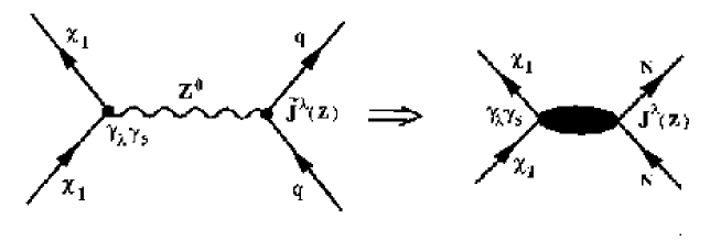
Figure 1: The LSP-quark interaction mediated by Z-exchange.

Using Eq. (3) and the fact that for Majorana particles ${\bar{\chi}}\gamma_{\mu}\chi=0$, we obtain

$${\it L}=\frac{g}{cos\theta_{W}}\frac{1}{4}(|C_{31}|^{2}-|C_{41}|^{2}){\bar{\chi}}_{1}\gamma_{\mu}\gamma_{5}\chi_{1}Z^{\mu}$$ (6)

which leads to the effective 4-fermion interaction

$${\it L}_{eff}=\frac{g}{cos\theta_{W}}\frac{1}{4}2(|C_{31}|^{2}-|C_{41}|^{2})(-\frac{g}{2cos\theta_{W}}\frac{1}{q^{2}-m^{2}_{Z}}{\bar{\chi}}_{1}\gamma^{\mu}\gamma_{5}\chi_{1})J^{Z}_{\mu}$$ (7)

where the extra factor of 2 comes from the Majorana nature of $\chi_{1}$. The neutral hadronic current $J^{Z}_{\lambda}$ is given by

$$J^{Z}_{\lambda}=-{\bar{q}}\gamma_{\lambda}\{\frac{1}{3}sin^{2}\theta_{W}-\Big{[}\,\frac{1}{2}(1-\gamma_{5})-sin^{2}\theta_{W}\Big{]}\tau_{3}\}q$$ (8)

at the nucleon level it can be written as

$${\tilde{J}}_{\lambda}^{Z}=-{\bar{N}}\gamma_{\lambda}\{\,sin^{2}\theta_{W}-g_{V}(\frac{1}{2}-sin^{2}\theta_{W})\tau_{3}+\frac{1}{2}g_{A}\gamma_{5}\tau_{3}\}N$$ (9)

Thus we can write

$${\it L}_{eff}=-\frac{G_{F}}{\sqrt{2}}({\bar{\chi}}_{1}\gamma^{\lambda}\gamma^{5}\chi_{1})J_{\lambda}(Z)$$ (10)

where

$$J_{\lambda}(Z)={\bar{N}}\gamma_{\lambda}[f^{0}_{V}(Z)+f^{1}_{V}(Z)\tau_{3}+f^{0}_{A}(Z)\gamma_{5}+f^{1}_{A}(Z)\gamma_{5}\tau_{3}]N$$ (11)

and

$$f^{0}_{V}(Z) = 2(|C_{31}|^{2}-|C_{41}|^{2})\frac{m^{2}_{Z}}{m^{2}_{Z}-q^{2}}sin^{2}\theta_{W}$$ (12)

$$f^{1}_{V}(Z) = -2(|C_{31}|^{2}-|C_{41}|^{2})\frac{m^{2}_{Z}}{m^{2}_{Z}-q^{2}}g_{V}(\frac{1}{2}-sin^{2}\theta_{W})$$ (13)

$$f^{0}_{A}(Z) = 0~{}~{},~{}~{}f^{1}_{A}(Z)=2(|C_{31}|^{2}-|C_{41}|^{2})\frac{m^{2}_{Z}}{m^{2}_{Z}-q^{2}}\,\,\frac{1}{2}g_{A}$$ (14)

with $g_{V}=1.0$ and $g_{A}=1.24$. We can easily see that

$$f^{1}_{V}(Z)/f^{0}_{V}(Z)=-g_{V}(\frac{1}{2sin^{2}\theta_{W}}-1)\simeq-1.15$$

Note that the suppression of this Z-exchange interaction compared to the ordinary neutral current interactions arises from the smallness of the mixing $C_{31}$ and $C_{41}$, a consequence of the fact that the Higgsinos are normally quite a bit heavier than the gauginos. Furthermore, the two Higgsinos tend to cancel each other.

We should also mention that the vector contribution, the time component of which can lead to coherence, contributes only to order $\upsilon/c\approx 10^{-3}$ due to the Majorana nature of the LSP. Thus to leading order only the axial current can contribute to the direct detection of the neutralino.

3.2 The $s$-quark Mediated Interaction

The other interesting possibility arises from the other two components of $\chi_{1}$, namely ${\tilde{B}}$ and ${\tilde{W}}_{3}$. Their corresponding couplings to $s$-quarks (see Fig. 2) can be read from the appendix C4 of Ref. Hab-Ka

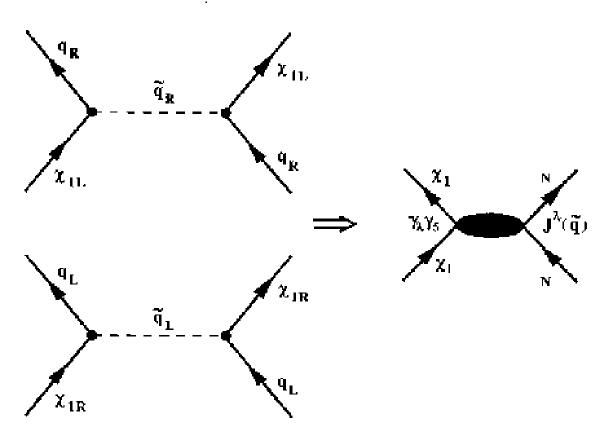
Figure 2: The LSP-quark interaction mediated by s-quark exchange.

They are

$${\it L}_{eff} = -g\sqrt{2}\{{\bar{q}}_{L}[T_{3}{\tilde{W}}_{3R}-tan\theta_{W}(T_{3}-Q){\tilde{B}}_{R}]{\tilde{q}}_{L}$$ (15)

$$- tan\theta_{W}{\bar{q}}_{R}Q{\tilde{B}}_{L}{\tilde{q}}_{R}\}+HC$$

where ${\tilde{q}}$ are the scalar quarks (SUSY partners of quarks). A summation over all quark flavors is understood. Using Eq. (3) we can write the above equation in the $\chi_{i}$ basis. Of interest to us here is the part

$${\it L}_{eff} = g\sqrt{2}\{(tan\theta_{W}(T_{3}-Q)C^{R}_{11}-T_{3}C^{R}_{21}){\tilde{q}}_{L}\chi_{1R}{\tilde{q}}_{L}$$ (16)

$$+ tan\theta_{W}C_{11}Q{\bar{q}}_{R}\chi_{1L}{\tilde{q}}_{R}\}$$

The above interaction is almost diagonal in the quark flavor. There exists, however, mixing between the s-quarks ${\tilde{q}}_{L}$ and ${\tilde{q}}_{R}$ (of the same flavor) i.e.

$${\tilde{q}}_{L}=cos\theta_{{\tilde{q}}}{\tilde{q}}_{1}+sin\theta_{{\tilde{q}}}{\tilde{q}}_{2}~{},~{}{\tilde{q}}_{R}=-sin\theta_{{\tilde{q}}}{\tilde{q}}_{1}+cos\theta_{{\tilde{q}}}{\tilde{q}}_{2}$$ (17)

with

$$tan2\theta_{{\tilde{u}}}=\frac{m_{u}(A+\mu cot\beta)}{m^{2}_{u_{L}}-m^{2}_{{\tilde{u}}_{R}}+m^{2}_{z}cos2\beta/2}~{},~{}tan2\theta_{{\tilde{d}}}=\frac{m_{d}(A+\mu tan\beta)}{m^{2}_{d_{R}}-m^{2}_{{\tilde{d}}_{R}}+m^{2}_{Z}cos2\beta/2}$$ (18)

Thus Eq. (16) becomes

$${\it L}_{eff} = g\sqrt{2}\left\{[B_{L}cos\theta_{{\tilde{q}}}\right.{\bar{q}}_{L}\chi_{1R}-B_{R}sin\theta_{{\tilde{q}}}{\bar{q}}_{R}\chi_{1L}]{\tilde{q}}_{1}$$

$$+ [B_{L}sin\theta_{{\tilde{q}}}{\bar{q}}_{L}\chi_{1R}+B_{R}cos\theta_{{\tilde{q}}}{\bar{q}}_{R}\chi_{1L}]\left.{\tilde{q}}_{2}\right\}$$

with

$B_{L}(q)=-\frac{1}{6}C^{R}_{11}tan\theta_{\omega}-\frac{1}{2}C^{R}_{21},\,\,\,q=u\ \ (charge\ \ 2/3)$

$B_{L}(q)=-\frac{1}{6}C^{R}_{11}tan\theta_{\omega}+\frac{1}{2}C^{R}_{21},\ \ \ q=d\ \ (charge\ \ -1/3)$

$B_{R}(q)=\frac{2}{3}tan\theta_{\omega}C_{11},\ \ \ q=u\ \ (charge\ \ 2/3)$

$B_{R}(q)=-\frac{1}{3}tan\theta_{\omega}C_{11},\ \ \ q=d\ \ (charge\ \ -1/3)$

The effective four fermion interaction takes the form

$${\it L}_{eff}=(g\sqrt{2})^{2}\{(B_{L}cos\theta_{\tilde{q}}{\bar{q}}_{L}\chi_{1R}-B_{R}sin\theta_{\tilde{q}}{\bar{q}}_{R}\chi_{1L})$$ (19)

$$\frac{1}{q^{2}-m_{{\tilde{q}}_{1}^{2}}}(B_{L}cos\theta_{q}{\bar{\chi}}_{1R}q_{L}-B_{R}sin\theta_{{\tilde{q}}}{\bar{\chi}}_{1L}q_{R})$$

$$+(B_{L}sin\theta_{q}q_{L}\chi_{1R}+cos\theta_{\tilde{q}}{\bar{q}}_{R}\chi_{1L})\frac{1}{q^{2}-m_{{\tilde{q}}_{2}^{2}}}$$

$$(B_{L}sin\theta_{q}{\bar{\chi}}_{1R}q_{L}+B_{R}cos\theta_{\tilde{q}}{\bar{\chi}}_{1L}q_{R})\}$$

The above effective interaction can be written as

$${\it L}_{eff}={\it L}_{eff}^{LL+RR}+{\it L}_{eff}^{LR}$$ (20)

The first term involves quarks of the same chirality and is not much effected by the mixing (provided that it is small). The second term involves quarks of opposite chirality and is proportional to the s-quark mixing.

The part ${\it L}_{eff}^{LL+RR}$

Employing a Fierz transformation ${\it L}_{eff}^{LL+RR}$ can be cast in the more convenient form

$${\it L}_{eff}^{LL+RR}= (g\sqrt{2})^{2}2(-\frac{1}{2})\{|B_{L}|^{2}$$ (21)

$$(\frac{cos^{2}\theta_{\tilde{q}}}{q^{2}-m_{{\tilde{q}}_{1}^{2}}}+\frac{sin^{2}\theta_{\tilde{q}}}{q^{2}-m_{{\tilde{q}}_{2}^{2}}}){\bar{q}}_{L}\gamma_{\lambda}q_{L}\chi_{1R}\gamma^{\lambda}\chi_{1R}$$

$$+|B_{R}|^{2}(\frac{sin^{2}\theta_{\tilde{q}}}{q^{2}-m_{{\tilde{q}}_{1}^{2}}}+\frac{cos^{2}{\theta_{\tilde{q}}}}{q^{2}-m_{{\tilde{q}}_{2}^{2}}}){\bar{q}}_{R}\gamma_{\lambda}q_{R}\chi_{1L}\gamma^{\lambda}\chi_{1L}\}$$

The factor of 2 comes from the Majorana nature of LSP and the (-1/2) comes from the Fierz transformation. Equation (21) can be written more compactly as

$${\it L}_{eff} = -\frac{G_{F}}{\sqrt{2}}2\{{\bar{q}}\gamma_{\lambda}(\beta_{0R}+\beta_{3R}\tau_{3})(1+\gamma_{5})q$$ (22)

$$- {\bar{q}}\gamma_{\lambda}(\beta_{0L}+\beta_{3L}\tau_{3})(1-\gamma_{5})q\}({\bar{\chi}}_{1}\gamma^{\lambda}\gamma^{5}\chi_{1}\}$$

with

$$\beta_{0R} = \Big{(}\frac{4}{9}\chi^{2}_{{\tilde{u}}_{R}}+\frac{1}{9}\chi^{2}_{{\tilde{d}}_{R}}\Big{)}|C_{11}tan\theta_{W}|^{2}$$

$$\beta_{3R} = \Big{(}\frac{4}{9}\chi^{2}_{{\tilde{u}}_{R}}-\frac{1}{9}\chi^{2}_{{\tilde{d}}_{R}}\Big{)}|C_{11}tan\theta_{W}|^{2}$$ (23)

$$\beta_{0L} = |\frac{1}{6}C^{R}_{11}tan\theta_{W}+\frac{1}{2}C^{R}_{21}|^{2}\chi^{2}_{{\tilde{u}}_{L}}+|\frac{1}{6}C^{R}_{11}tan\theta_{W}-\frac{1}{2}C^{R}_{21}|^{2}\chi^{2}_{{\tilde{d}}_{L}}$$

$$\beta_{3L} = |\frac{1}{6}C^{R}_{11}tan\theta_{W}+\frac{1}{2}C^{R}_{21}|^{2}\chi^{2}_{{\tilde{u}}_{L}}-|\frac{1}{6}C^{R}_{11}tan\theta_{W}-\frac{1}{2}C^{R}_{21}|^{2}\chi^{2}_{{\tilde{d}}_{L}}$$

with

$$\chi^{2}_{qL}=c^{2}_{\tilde{q}}\frac{m_{W}^{2}}{m_{{\tilde{q}}^{2}_{1}}-q^{2}}+s^{2}_{{\tilde{q}}}\frac{m_{W}^{2}}{m_{{\tilde{q}}^{2}_{2}}-q^{2}}~{}~{},~{}~{}\chi^{2}_{qR}=s^{2}_{\tilde{q}}\frac{m_{W}^{2}}{m_{{\tilde{q}}^{2}_{1}}-q^{2}}+c^{2}_{\tilde{q}}\frac{m_{W}^{2}}{m_{{\tilde{q}}^{2}_{2}}-q^{2}}$$ (24)

where $c_{\tilde{q}}=cos\theta_{\tilde{q}},\,\ s_{\tilde{q}}=sin\theta_{\tilde{q}}$. The above parameters are functions of the four-momentum transfer which in our case is negligible.
Eq (22) it is often written as:

$${\it L}_{eff}=-\frac{G_{F}}{\sqrt{2}}2\ \left[{\bar{u}}\gamma_{\lambda}(d^{0}(u)+\gamma_{5}d(u))u+{\bar{d}}\gamma_{\lambda}(d^{0}(d)+\gamma_{5}d(d))d\right]({\bar{\chi}}_{1}\gamma^{\lambda}\gamma^{5}\chi_{1}\}$$ (25)

where

$$d^{0}(u)=\beta_{0R}+\beta_{3R}-\beta_{0L}-\beta_{3L},d(u)=\beta_{0R}+\beta_{3R}+\beta_{0L}+\beta_{3L}$$ (26)

$$d^{0}(d)=\beta_{0R}-\beta_{3R}-\beta_{0L}+\beta_{3L},d(u)=\beta_{0R}-\beta_{3R}+\beta_{0L}-\beta_{3L}$$ (27)

Proceeding as in sec. 3.1 we can obtain the effective Lagrangian at the nucleon level as

$${\it L}_{eff}^{LL+RR}=-\frac{G_{F}}{\sqrt{2}}({\bar{\chi}}_{1}\gamma^{\lambda}\gamma^{5}\chi_{1})J_{\lambda}({\tilde{q}})$$ (28)

$$J_{\lambda}({\tilde{q}})={\bar{N}}\gamma_{\lambda}\{f^{0}_{V}({\tilde{q}})+f^{1}_{V}({\tilde{q}})\tau_{3}+f^{0}_{A}({\tilde{q}})\gamma_{5}+f^{1}_{A}({\tilde{q}})\gamma_{5}\tau_{3})N$$ (29)

with

$$f^{0}_{V}=6(\beta_{0R}-\beta_{0L}),\qquad f^{1}_{V}=2g_{V}(\beta_{3R}-\beta_{3L})$$

$$f^{0}_{A}=2g^{0}_{A}(\beta_{0R}+\beta_{0L}),\qquad f^{1}_{A}=2g_{A}(\beta_{3R}+\beta_{3L})$$ (30)

with $g_{v}=1.0$ and $g_{A}=1.25$. The quantity $g^{0}_{A}$ depends on the quark model for the nucleon. It can be anywhere between 0.12 and 1.00 (see below 4.2).

We should note that this interaction is more suppressed than the ordinary weak interaction by the fact that the masses of the s-quarks are usually larger than that of the gauge boson $Z^{0}$. In the limit in which the LSP is a pure bino ($C_{11}=1,C_{21}=0$) we obtain

$$\beta_{0R}=tan^{2}\theta_{W}\Big{(}\frac{4}{9}\chi^{2}_{u_{R}}+\frac{1}{9}\chi^{2}_{{\tilde{d}}_{R}}\Big{)}~{},~{}\beta_{3R}=tan^{2}\theta_{W}\Big{(}\frac{4}{9}\chi^{2}_{u_{R}}-\frac{1}{9}\chi^{2}_{{\tilde{d}}_{R}}\Big{)}$$ (31)

$$\beta_{0L}=\frac{tan^{2}\theta_{W}}{36}(\chi^{2}_{{\tilde{u}}_{L}}+\chi^{2}_{{\tilde{d}}_{L}})~{},~{}\beta_{3L}=\frac{tan^{2}\theta_{W}}{36}(\chi^{2}_{{\tilde{u}}_{L}}-\chi^{2}_{{\tilde{d}}_{L}})$$ (32)

Assuming further that $\chi_{{\tilde{u}}_{R}}=\chi_{{\tilde{d}}_{R}}=\chi_{{\tilde{u}}_{L}}=\chi_{{\tilde{d}}_{L}}$ we obtain

$$f^{1}_{V}({\tilde{q}})/f^{0}_{V}({\tilde{q}})\simeq+\frac{2}{9}~{},~{}f^{1}_{A}({\tilde{q}})/f^{0}_{A}({\tilde{q}})\simeq+\frac{6}{11}$$ (33)

If, on the other hand, the LSP were the photino ($C_{11}=cos\theta_{W},C_{21}=sin\theta_{W},C_{31}=C_{41}=0$) and the s-quarks were degenerate there would be no coherent contribution ($f^{0}_{V}=0$ if $\beta_{0L}=\beta_{0R}$).

As we have mentioned in the previous section, to leading order, only the axial current contributes to the direct detection of the neutralino.

The part ${\it L}_{eff}^{LR}$

From Eq. (19) we obtain

$${\it L}_{eff}^{LR} = -(g\sqrt{2})^{2}sin2\theta_{\tilde{q}}B_{L}(q)B_{R}(q)\frac{1}{2}[\frac{1}{q^{2}-m_{{\tilde{q}}_{1}^{2}}}-\frac{1}{q^{2}-m_{{\tilde{q}}_{2}^{2}}}]$$

$$({\bar{q}}_{L}\chi_{1R}{\bar{\chi}}_{1L}q_{R}+{\bar{q}}_{R}\chi_{1L}{\bar{\chi}}_{1R}q_{L})$$

Employing a Fierz transformation we can cast it in the form

$${\it L}_{eff}=-\frac{G_{F}}{\sqrt{2}}\sum_{q}\beta(q)\left[({\bar{q}}q{\bar{\chi}}_{1}\chi_{1}+{\bar{q}}\gamma_{5}q{\bar{\chi}}_{1}\gamma_{5}\chi_{1}-({\bar{q}}\sigma_{\mu\nu}q)({\bar{\chi}}_{1}\sigma^{\mu\nu}\chi_{1}))\right]$$ (35)

where

$$\beta(u)=\frac{2}{3}tan\theta_{W}C_{11}\{2sin2\theta_{\tilde{u}}[\frac{1}{6}CR_{11}tan\theta_{W}+\frac{1}{2}CR_{21}]\Delta_{\tilde{u}}$$ (36)

$$\beta(d)=sin2\theta_{\tilde{d}}[\frac{1}{6}CR_{11}tan\theta_{W}-\frac{1}{2}C^{R}_{21}]\Delta_{\tilde{d}}\}$$ (37)

Where in the last expressions $u$ indicates quarks with charge 2/3 and d quarks with charge -1/3. In all cases

$\Delta_{\tilde{u}}=\frac{(m^{2}_{{\tilde{u}}_{1}}-m^{2}_{{\tilde{u}}_{2}})M^{2}_{W}}{(m^{2}_{{\tilde{u}}_{1}}-q^{2})(m^{2}_{{\tilde{u}}_{2}}-q^{2})}$

and an analogous equation for $\Delta_{\tilde{d}}$.

The appearance of scalar terms in s-quark exchange ref1 has been first noticed by Griest GRIEST . It has also been noticed there that one should consider explicitly the effects of quarks other than u and d Dree in going from the quark to the nucleon level. We first notice that with the exception of $t$ s-quark the ${\tilde{q}}_{L}-{\tilde{q}}_{R}$ mixing small. Thus

$$sin2\theta_{\tilde{u}}\Delta{\tilde{u}}\simeq\frac{2m_{u}(A+\mu cot\beta)m^{2}_{W}}{(m^{2}_{{\tilde{u}}_{L}}-q^{2})(m^{2}_{{\tilde{u}}_{R}}-q^{2})}~{},~{}sin2\theta_{\tilde{d}}\Delta{\tilde{d}}\simeq\frac{2m_{d}(A+\mu tan\beta)m^{2}_{W}}{(m^{2}_{{\tilde{d}}_{L}}-q^{2})(m^{2}_{{\tilde{d}}_{R}}-q^{2})}$$ (38)

In going to the nucleon level and ignoring the negligible pseudoscalar and tensor components we only need modify the above expressions for all quarks, with the possible exception of the $t$ quarks, by the substitution $m_{q}\rightarrow f_{q}m_{N}$ (see sec. 4.1). For the t s-quark the mixing is complete, which implies that the amplitude is independent of the top quark mass. Hence in the case of the top quark we may not get an extra enhancement in going from the quark to the nucleon level. In any case this way we get

$${\it L}_{eff}=\frac{G_{F}}{\sqrt{2}}[f^{0}_{S}({\tilde{q}}){\bar{N}}N+f^{1}_{S}({\tilde{q}}){\bar{N}}\tau_{3}N]{\bar{\chi}}_{1}\chi_{1}$$ (39)

with

$$f^{0}_{S}({\tilde{q}})=\frac{f_{u}\beta(u)+f_{d}\beta(d)}{2}+\sum_{q=s,c,b,t}f_{q}\beta(q)$$ (40)

$$f^{1}_{S}({\tilde{q}})=\frac{f_{u}\beta(u)-f_{d}\beta(d)}{2}$$ (41)

(see sec. 4.1 for details). In the allowed SUSY parameter space considered in this work this contribution can be neglected in front of the Higgs exchange contribution. This happens because for quarks other than t the s-quark mixing is small. For the t-quark, as it has already been mentioned, we have large mixing, but we do not get the advantage of the mass enhancement.

3.3 The Intermediate Higgs Contribution

The coherent scattering can be mediated via the intermediate Higgs particles which survive as physical particles (see Fig. 3).

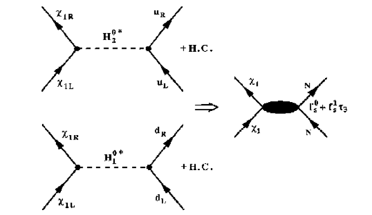
Figure 3: The LSP-quark interaction mediated by Higgs exchange.

The relevant interaction can arise out of the Higgs-Higgsino-gaugino interaction which takes the form

$${\it L}_{H\chi\chi} = \frac{g}{\sqrt{2}}\Big{(}{\bar{\tilde{W}}}^{3}_{R}{\tilde{H}}_{2L}H^{0*}_{2}-{\bar{\tilde{W}}}^{3}_{R}{\tilde{H}}_{1L}H^{0*}_{1}$$ (42)

$$- tan\theta_{w}({\bar{\tilde{B}}}_{R}{\tilde{H}}_{2L}H^{0*}_{2}-{\bar{\tilde{B}}}_{R}{\tilde{H}}_{1L}H^{0*}_{1})\Big{)}+H.C.$$

Proceeding as above we can express ${\tilde{W}}$ an ${\tilde{B}}$ in terms of the appropriate eigenstates and retain the LSP to obtain

$${\it L} = \frac{g}{\sqrt{2}}\Big{(}(C^{R}_{21}-tan\theta_{w}C^{R}_{11})C_{41}{\bar{\chi}}_{1R}\chi_{1L}H^{o*}_{2}$$ (43)

$$- (C^{R}_{21}-tan\theta_{w}C^{R}_{11})C_{31}{\bar{\chi}}_{1R}\chi_{1L}H^{o*}_{1}\Big{)}+H.C.$$

We can now proceed further and express the fields ${H^{0}_{1}}^{*}$, ${H^{0}_{2}}^{*}$ in terms of the physical fields $h$, $H$ and $A.$ The term which contains $A$ will be neglected, since it yields only a pseudoscalar coupling which does not lead to coherence.

Thus we can write

$${\cal L}_{eff}=-\frac{G_{F}}{\sqrt{2}}{\bar{\chi}}\chi\,{\bar{N}}[f^{0}_{s}(H)+f^{1}_{s}(H)\tau_{3}]N$$ (44)

where

$$f^{0}_{S}(H)=\frac{1}{2}(g_{u}+g_{d})+g_{s}+g_{c}+g_{b}+g_{t}$$ (45)

$$f^{1}_{S}(H)=\frac{1}{2}(g_{u}-g_{d})$$ (46)

with

$$g_{a_{i}}=\big{[}g_{1}(h)\frac{cos\alpha}{sin\beta}+g_{2}(H)\frac{sin\alpha}{sin\beta}\big{]}\frac{m_{a_{i}}}{m_{N}},\quad a_{i}=u,c,t$$ (47)

$$g_{\kappa_{i}}=\big{[}-g_{1}(h)\frac{sin\alpha}{cos\beta}+g_{2}(H)\frac{cos\alpha}{cos\beta}\big{]}\frac{m_{\kappa_{i}}}{m_{N}},\quad\kappa_{i}=d,s,b$$ (48)

$$g_{1}(h)=4(C^{R}_{11}tan\theta_{W}-C^{R}_{21})(C_{41}cos\alpha+C_{31}sin\alpha)\frac{m_{N}m_{W}}{m^{2}_{h}-q^{2}}$$ (49)

$$g_{2}(H)=4(C^{R}_{11}tan\theta_{W}-C^{R}_{21})(C_{41}sin\alpha-C_{31}cos\alpha)\frac{m_{N}m_{W}}{m^{2}_{H}-q^{2}}$$ (50)

where $m_{N}$ is the nucleon mass, and the parameters $m_{h}$, $m_{H}$ and $\alpha$ depend on the SUSY parameter space (see Table 1).

4 Going from the Quark to the Nucleon Level

As we have already mentioned, one has to be a bit more careful in handling quarks other than $u$ and $d$.

4.1 The scalar interaction

As we have seen the scalar couplings of the LSP to the quarks are proportional to their mass Dree . One encounters in the nucleon not only sea quarks ($u{\bar{u}},d{\bar{d}}$ and $s{\bar{s}}$) but the heavier quarks also due to QCD effects  Dree00 . This way one obtains the scalar Higgs-nucleon coupling by using effective parameters $f_{q}$ defined as follows:

$$\Big{<}N|m_{q}\bar{q}q|N\Big{>}=f_{q}m_{N}$$ (51)

where $m_{N}$ is the nucleon mass. The parameters $f_{q},~{}q=u,d,s$ can be obtained by chiral symmetry breaking terms in relation to phase shift and dispersion analysis. The isoscalar component can be obtained by considering the following quantities :

1. The phenomenologically determined mass ratios:

   $$\frac{m_{u}}{m_{d}}=0.553\pm 0.043~{}~{},~{}~{}\frac{m_{s}}{m_{d}}=18.9\pm 0.08$$ (52)

2. The quantities :

   $$z=\frac{B_{u}-B_{s}}{B_{d}-B_{s}}\approx 1.49~{}~{},~{}~{}y=\frac{2B_{s}}{B_{d}+B_{u}}$$ (53)

   One then finds that:

   $$\frac{B_{u}}{B_{d}}=\frac{2z-(z-1)y}{2+(z-1)y}\mbox{ for protons}~{},~{}\frac{B_{u}}{B_{d}}=\frac{2+(z-1)y}{2z-(z-1)y}\mbox{ for neutrons}$$ (54)

   with $B_{q}=<N|\bar{q}q|N>$

3. The pion-nucleon sigma-term, $\sigma_{\pi N}$:
   this term is obtained from the isospin even $\pi$-N scattering amplitude with vanishing external momenta. It is defined by the scalar quark density operator averaged over the nucleon or equivalently by $\sigma_{\pi N}(t=0)$, the scalar form factor of the nucleon at zero momentum transfer squared. The value of the sigma term is deduced from the analysis of two quantities: $\sigma_{\pi N}(t=2M_{\pi}^{2})$ the scalar form factor at the Cheng-Dashen point, which is experimentally accessible, and the difference $\Delta_{\sigma}=\sigma_{\pi N}(2M_{\pi}^{2})-\sigma_{\pi N}(0)=15.2\pm 0.4$ MeV SAINIO91 ,GASSER82 as induced by explicit chiral symmetry breaking. Experimentally, after efforts of many years, the value of the sigma-tern is still quite uncertain GASSER82 . The canonical value of the $\pi N$ sigma term with

   $$\sigma_{\pi N}={m_{u}+m_{d}\over 2}(B_{u}+B_{d})=(45\pm 8)~{}MeV$$ (55)

   is deduced from an earlier analyses with $\sigma_{\pi N}(t=2M_{\pi}^{2})=60\pm 8$ SAINIO91 . During the last few years analyses of also more recent pion-nucleon scattering data lead to an increase in the value of scalar form factor at the Cheng-Dashen point $\sigma_{\pi N}(M_{\pi}^{2})$ with $88\pm 15$ MeV Kaufmann:dd , $71\pm 9$ MeV Olsson:1999jt , $79\pm 7$ MeV Pavan:2001wz and $(80-90)$ MeV Olsson:2002 . Thus the recent analyses suggest a value for the pion-nucleon sigma term of about

   $$\sigma_{\pi N}={m_{u}+m_{d}\over 2}(B_{u}+B_{d})=(56-75)~{}MeV$$ (56)

   .

4. Theoretical analysis of the $\sigma_{\pi N}$ term:
   In the context of chiral perturbation one can show that:

   $$\sigma_{\pi N}={\sigma_{0}\over 1-y}~{},~{}\sigma_{0}=(35\pm 5)~{}MeV$$ (57)

   Eqs. (55) and (56) together with Eq. (57) will provide the range of variation in the parameter y. Taking:

   $$m_{u}=5.1~{}MeV~{}~{},m_{d}=9.3~{}MeV$$ (58)

   together with y will in turn provide by Eq. 54 the range of variation of the ratio $B_{u}/B_{d}$. The uncertainties in Eqs. (55,56,57) provide a wide range in which the parameter y can vary. In other words the experimental and theoretical uncertainties permit us, we will exploit the possible consequences of variation in y to SUSY dark matter detection. For $\sigma_{\pi N}$ we choose $45,~{}55,~{}65$ and $75$ MeV to reflect the range of values set by Eqs. (55) and (56). Thus from Eq. (57) we extract the corresponding y parameters with $0.22\pm 0.11,~{}0.36\pm 0.09,~{}046\pm 0.08$ and $0.53\pm 0.07$, respectively. Then we will combine these values with Eq. 54 to get the desired values of $f_{q}$ given below.

From the above analysis we get in the case of the proton:

$$f^{p}_{d}=\frac{\Sigma_{\pi N}}{0.756~{}m_{p}}[1+\frac{2z-(z-1)y}{2+(z-1)y}]^{-1}$$ (59)

$$f^{p}_{u}=0.553~{}f^{p}_{d}~{}[\frac{2z-(z-1)y}{2+(z-1)y}]~{},~{}f^{p}_{s}=\frac{\Sigma_{\pi N}}{0.756~{}m_{p}}~{}\frac{19}{2}~{}y$$ (60)

$$f^{p}_{s}=\frac{\Sigma_{\pi N}}{0.756~{}m_{p}}~{}\frac{19}{2}~{}y$$ (61)

In the case of the neutron our expressions are analogous, the ratio $B_{u}/B_{d}$ getting the inverse value.
For the heavy quarks, to leading order via quark loops and gluon exchange with the nucleon, one finds:

$f_{Q}=2/27(1-\quad\sum_{q}f_{q})$

There is a correction to the above parameters coming from loops involving s-quarks Dree00 . The leading contribution can be absorbed into the definition, if the functions $g_{1}(h)$ and $g_{2}(H)$ as follows :

$g_{1}(h)\rightarrow g_{1}(h)[1+\frac{1}{8}(2\frac{m^{2}_{Q}}{m^{2}_{W}}-\frac{sin(\alpha+\beta)}{cos^{2}\theta_{W}}\frac{sin\beta}{cos\alpha})]$

$g_{2}(H)\rightarrow g_{1}(h)[1+\frac{1}{8}(2\frac{m^{2}_{Q}}{m^{2}_{W}}+\frac{cos(\alpha+\beta)}{cos^{2}\theta_{W}}\frac{sin\beta}{sin\alpha})]$

for $Q=c$ and $t$ For the b-quark we get:

$g_{1}(h)\rightarrow g_{1}(h)[1+\frac{1}{8}(2\frac{m^{2}_{b}}{m^{2}_{W}}-\frac{sin(\alpha+\beta)}{cos^{2}\theta_{W}}\frac{cos\beta}{cos\alpha})]$

$g_{2}(H)\rightarrow g_{1}(h)[1+\frac{1}{8}(2\frac{m^{2}_{b}}{m^{2}_{W}}-\frac{cos(\alpha+\beta)}{cos^{2}\theta_{W}}\frac{cos\beta}{sin\alpha})]$

In addition to the above effects one has to consider QCD effects. These effects renormalize the contribution of the quark loops as follows Dree00 :

$f_{QCD}(q)=\frac{1}{4}\frac{\beta(\alpha_{s})}{1+\gamma_{m}(\alpha_{s})}$

with

$\beta(\alpha_{s})=\frac{\alpha_{s}}{3\pi}[1+\frac{19}{4}{\alpha_{s}}{\pi}]$ , $\gamma_{m}(\alpha_{s})=2\frac{\alpha_{s}}{\pi}$

Thus

$f_{QCD}(q)=1+\frac{11}{4}\frac{\alpha_{s}}{\pi}$

The QCD correction associated with the s-quark loops is:

$f_{QCD}(\tilde{q})=1+\frac{25}{6}\frac{\alpha_{s}}{\pi}$

The above corrections depend on Q since $\alpha_{s}$ must be evaluated at the scale of $m_{Q}$.
It convenient to introduce the factor$f_{QCD}(\tilde{q})/f_{QCD}(q)$ into the factors $g_{1}(h)$ and $g_{2}(H)$ and the factor of $f_{QCD}(q)$ into the the quantities $f_{Q}$. If, however, one restricts oneself to the large $tan\beta$ regime, the corrections due to the s-quark loops is independent of the parameters $\alpha$ and $\beta$ and significant only for the t-quark.

For a more detailed discussion we refer the reader to Refs. Dree ; Dree00 . We thus obtain the results presented in Table 1.

Table 1: The parameters $f^{p}_{q}$ and $f^{p}_{Q}$ (upper part) as well as $f^{n}_{q}$ and $f^{n}_{Q}$ (lower part) for the twelve cases discussed in the text.

$\#$	$f^{p}_{d}$	$f^{p}_{u}$	$f^{p}_{s}$	$f^{p}_{c}$	$f^{p}_{b}$	$f^{p}_{t}$		$f^{n}_{d}$	$f^{n}_{u}$	$f^{n}_{s}$	$f^{n}_{c}$	$f^{n}_{b}$	$f^{n}_{t}$
1	0.026	0.021	0.067	0.098	0.104	0.161		0.037	0.014	0.066	0.098	0.104	0.161
2	0.027	0.020	0.133	0.087	0.092	0.144		0.037	0.015	0.133	0.086	0.092	0.143
3	0.028	0.020	0.199	0.075	0.080	0.126		0.036	0.015	0.199	0.075	0.080	0.126
4	0.033	0.025	0.199	0.078	0.083	0.132		0.044	0.018	0.199	0.077	0.083	0.122
5	0.034	0.024	0.265	0.068	0.072	0.117		0.044	0.019	0.265	0.067	0.172	0.117
6	0.031	0.025	0.332	0.057	0.061	0.106		0.043	0.017	0.332	0.057	0.062	0.102
7	0.040	0.028	0.331	0.061	0.065	0.109		0.051	0.022	0.331	0.060	0.065	0.109
8	0.041	0.028	0.400	0.051	0.055	0.095		0.051	0.023	0.400	0.050	0.055	0.095
9	0.047	0.028	0.470	0.041	0.047	0.081		0.051	0.023	0.400	0.050	0.055	0.095
10	0.047	0.027	0.462	0.045	0.050	0.090		0.050	0.023	0.470	0.040	0.044	0.060
11	0.048	0.032	0.532	0.036	0.040	0.076		0.058	0.027	0.532	0.035	0.040	0.076
12	0.049	0.032	0.603	0.026	0.030	0.063		0.057	0.027	0.603	0.026	0.030	0.063

We notice that there exist differences between the proton and neutron components. These, however, cannot be taken as the sole contribution to isovector contribution, since all quantities were derived with isoscalar operators. So the isovector contribution will be discussed elsewhere. Here we will limit ourselves to the isoscalar component $f_{q}=(f^{p}_{q}+f^{n}_{q})/2$

4.2 The axial current contribution

The amplitudes $a_{p}=f^{0}_{A}+f^{1}_{A}$ and $a_{n}=f^{0}_{A}-f^{1}_{A}$ are defined by JELLIS :

$$a_{N}=\sum_{q=u,d,s}d_{q}\Delta q_{N}$$ (62)

$$2s_{\mu}\Delta q_{N}=\left<N|\bar{q}\gamma_{\mu}\gamma_{5}q|N\right>$$ (63)

where $s_{\mu}$ is the nucleon spin and $d_{q}$ the relevant spin amplitudes at the quark level obtained in a given SUSY model.
The isoscalar and the isovector axial current couplings at the nucleon level, $f^{0}_{A}$, $f^{1}_{A}$, are obtained from the corresponding ones given by the SUSY models at the quark level, $f^{0}_{A}(q)$, $f^{1}_{A}(q)$, via renormalization coefficients $g^{0}_{A}$, $g_{A}^{1}$, i.e. $f^{0}_{A}=g_{A}^{0}f^{0}_{A}(q),f^{1}_{A}=g_{A}^{1}f^{1}_{A}(q).$ The renormalization coefficients are given terms of $\Delta q$ defined above JELLIS , via the relations

$$g_{A}^{0}=\Delta u+\Delta d+\Delta s=0.77-0.49-0.15=0.13~{},~{}g_{A}^{1}=\Delta u-\Delta d=1.26$$

We see that, barring very unusual circumstances at the quark level, the isoscalar contribution is negligible. It is for this reason that one might prefer to work in the isospin basis.

5 The nucleon cross sections

With the above ingredients we are in a position to evaluate the nucleon cross sections.

• The scalar cross section. As we have mentioned this is primarily due to the Higgs exchange.

  $$\sigma^{S}_{p,\chi^{0}}=\sigma_{0}|{f^{0}_{S}}+{f^{1}_{S}}|^{2}~{},~{}\sigma^{S}_{n,\chi^{0}}=\sigma_{0}|{f^{0}_{S}}-{f^{1}_{S}}|^{2}$$ (64)

  with

  $$\sigma_{0}=\frac{1}{2\pi}(G_{F}m_{p})^{2}=0.77\times 10^{-38}cm^{2}=0.77\times 10^{-2}pb$$ (65)

  Since, however, the process is dominated by quarks other than $u$ and $d$, the isovector contribution is negligible. So we can talk about the nucleon cross section.

• The proton spin cross section is given by:

  $$\sigma^{spin}_{p,\chi^{0}}=3\sigma_{0}|{f^{0}_{A}}+{f^{1}_{A}}|^{2}=3\sigma_{0}|a_{p}|^{2}$$ (66)

6 The allowed SUSY Parameter Space

It is clear from the above discussion that the nucleon cross section depends:

• The the quark structure of the nucleon
  The allowed range of the parameters $f_{q}$ may induce variations in the nucleon cross section as large as an order of magnitude.

• The parameters of supersymmetry.
  This is the most crucial input. One starts with a set of parameters at the GUT scale and predicts the low energy observable via the renormalization group equations (RGE). Conversely starting from the low energy phenomenology one can constrain the input parameters at the GUT scale.

The parameter space is the most crucial. In SUSY models derived from minimal SUGRA the allowed parameter space is characterized at the GUT scale by five parameters:

• two universal mass parameters, one for the scalars, $m_{0}$, and one for the fermions, $m_{1/2}$.

• $tan\beta$.

• The trilinear coupling $A_{0}$ (or $m^{pole}_{t}$) and

• The sign of $\mu$ in the Higgs self-coupling $\mu H_{1}~{}H2$.

The experimental constraints are

1. The LSP relic abundance (including co-annihilations):

   $$0.09\leq\Omega_{LSP}h^{2}\leq 0.22\mbox{ (previous)},~{}0.09\leq\Omega_{LSP}h^{2}\leq 0.124\mbox{ (WMAP)}$$

2. the $b\rightarrow s\gamma$ constraint (CLEO, BELLE)

   $$2\times 10^{-4}\leq BR\leq 4.1\times 10^{-4}$$

3. The Higgs mass:$~{}~{}~{}\geq 114.1~{}GeV$. This applies on the standard model Higgs. So For SUSY one must correct for factor $\sin^{2}{(\alpha-\beta)}$ where $\alpha$ is the Higgs mixing angle. So this imposes limits on $\tan{\beta}$

4. Limits on $g_{s}-2$ $(e^{-},e^{+})$ experiments (E821 at BNL)

   $$a_{\mu}=(g_{\mu}-2)/2=(33.7\pm 11.2)\times 10^{-10}$$

   yields ($2\sigma$ level):

   $$11.3\times 10^{-10}\leq\delta a_{\mu}(SUGRA)\leq 56.1\times 10^{-10}$$

5. The fermion masses:
   $m_{t}(pole)=175~{}GeV~{},~{}m_{b}(m_{b})=4.25~{}GeV\Rightarrow$
   $m_{b}(m_{Z})=2.888~{}GeV,~{}m_{\tau}(M_{Z})=1.7463~{}GeV$

We are not going to elaborate further on this interesting aspect, since it will be covered by another contribution to these proceedings by A. Lahanas.

7 Rates

The differential non directional rate can be written as

$$dR_{undir}=\frac{\rho(0)}{m_{\chi}}\frac{m}{Am_{N}}d\sigma(u,\upsilon)|{\boldmath\upsilon}|$$ (67)

where A is the nuclear mass number, $\rho(0)\approx 0.3GeV/cm^{3}$ is the LSP density in our vicinity, m is the detector mass, $m_{\chi}$ is the LSP mass and $d\sigma(u,\upsilon)$ is the differential cross section.

The directional differential rate, i.e. that obtained, if nuclei recoiling in the direction $\hat{e}$ are observed, is given by JDVSPIN04 :

$$dR_{dir}=\frac{\rho(0)}{m_{\chi}}\frac{m}{Am_{N}}|\upsilon|\hat{\upsilon}.\hat{e}~{}\Theta(\hat{\upsilon}.\hat{e})~{}\frac{1}{2\pi}~{}d\sigma(u,\upsilon\ \delta(\frac{\sqrt{u}}{\mu_{r}\upsilon\sqrt{2}}-\hat{\upsilon}.\hat{e})$$

where $\Theta(x)$ is the Heaviside function.

The differential cross section is given by:

$$d\sigma(u,\upsilon)==\frac{du}{2(\mu_{r}b\upsilon)^{2}}[(\bar{\Sigma}_{S}F(u)^{2}+\bar{\Sigma}_{spin}F_{11}(u)]$$ (68)

where $u$ the energy transfer $Q$ in dimensionless units given by

$$u=\frac{Q}{Q_{0}}~{}~{},~{}~{}Q_{0}=[m_{p}Ab]^{-2}=40A^{-4/3}~{}MeV$$ (69)

with $b$ is the nuclear (harmonic oscillator) size parameter. $F(u)$ is the nuclear form factor and $F_{11}(u)$ is the spin response function associated with the isovector channel.

The scalar cross section is given by:

$$\bar{\Sigma}_{S}=(\frac{\mu_{r}}{\mu_{r}(p)})^{2}\sigma^{S}_{p,\chi^{0}}A^{2}\left[\frac{1+\frac{f^{1}_{S}}{f^{0}_{S}}\frac{2Z-A}{A}}{1+\frac{f^{1}_{S}}{f^{0}_{S}}}\right]^{2}\approx\sigma^{S}_{N,\chi^{0}}(\frac{\mu_{r}}{\mu_{r}(p)})^{2}A^{2}$$ (70)

(since the heavy quarks dominate the isovector contribution is negligible). $\sigma^{S}_{N,\chi^{0}}$ is the LSP-nucleon scalar cross section. The spin Cross section is given by:

$$\bar{\Sigma}_{spin}=(\frac{\mu_{r}}{\mu_{r}(p)})^{2}\sigma^{spin}_{p,\chi^{0}}~{}\zeta_{spin},\zeta_{spin}=\frac{1}{3(1+\frac{f^{0}_{A}}{f^{1}_{A}})^{2}}S(u)$$ (71)

$$S(u)\approx S(0)=[(\frac{f^{0}_{A}}{f^{1}_{A}}\Omega_{0}(0))^{2}+2\frac{f^{0}_{A}}{f^{1}_{A}}\Omega_{0}(0)\Omega_{1}(0)+\Omega_{1}(0))^{2}\,]$$ (72)

The couplings $f^{1}_{A}$ ($f^{0}_{A}$) and the nuclear matrix elements $\Omega_{1}(0)$ ($\Omega_{0}(0)$) associated with the isovector (isoscalar) components are normalized so that, in the case of the proton at $u=0$, they yield $\zeta_{spin}=1$.

With these definitions in the proton neutron representation we get:

$$\zeta_{spin}=\frac{1}{3}S^{{}^{\prime}}(0)$$ (73)

$$S^{{}^{\prime}}(0)=\left[(\frac{a_{n}}{a_{p}}\Omega_{n}(0))^{2}+2\frac{a_{n}}{a_{p}}\Omega_{n}(0)\Omega_{p}(0)+\Omega^{2}_{p}(0)\right]$$ (74)

where $\Omega_{p}(0)$ and $\Omega_{n}(0)$ are the proton and neutron components of the static spin nuclear matrix elements. In extracting limits on the nucleon cross sections from the data we will find it convenient to write:

$$\sigma^{spin}_{p,\chi^{0}}~{}\zeta_{spin}=\frac{\Omega^{2}_{p}(0)}{3}|\sqrt{\sigma_{p}}+\frac{\Omega_{n}}{\Omega_{p}}\sqrt{\sigma_{n}}e^{i\delta}|^{2}$$ (75)

In Eq. (75) $\delta$ the relative phase between the two amplitudes $a_{p}$ and $a_{n}$. The static spin matrix elements are obtained in the context of a given nuclear model. Some such matrix elements of interest to the planned experiments are given in table 2. The shown results are obtained from Divari DIVA00 , Ressel et al (*) Ress , the Finish group (**) SUHONEN03 and the Ioannina team (+) ref1 , KVprd .

Table 2: The static spin matrix elements for various nuclei. For ³He see Moulin, Mayet and Santos Santos ,SANTOS04 . For the other light nuclei the calculations are from DIVARI DIVA00 . For ⁷³Ge and ¹²⁷I the results presented are from Ressel et al Ress (*) and the Finish group et al SUHONEN03 (**). For ²⁰⁷Pb they were obtained by the Ioannina team (+). ref1 , KVprd .

	3 He	19F	29Si	23Na	73Ge	127I∗	127I∗∗	207Pb+
$\Omega_{0}(0)$	1.244	1.616	0.455	0.691	1.075	1.815	1.220	0.552
$\Omega_{1}(0)$	-1.527	1.675	-0.461	0.588	-1.003	1.105	1.230	-0.480
$\Omega_{p}(0)$	-0.141	1.646	-0.003	0.640	0.036	1.460	1.225	0.036
$\Omega_{n}(0)$	1.386	-0.030	0.459	0.051	1.040	0.355	-0.005	0.516
$\mu_{th}$		2.91	-0.50	2.22
$\mu_{exp}$		2.62	-0.56	2.22
$\frac{\mu_{th}(spin)}{\mu_{exp}}$		0.91	0.99	0.57

The spin ME are defined as follows:

$$\Omega_{p}(0)=\sqrt{\frac{J+1}{J}}\prec J~{}J|\sigma_{z}(p)|J~{}J\succ~{}~{},~{}~{}\Omega_{n}(0)=\sqrt{\frac{J+1}{J}}\prec J~{}J|\sigma_{z}(n)|J~{}J\succ$$ (76)

where $J$ is the total angular momentum of the nucleus and $\sigma_{z}=2S_{z}$. The spin operator is defined by $S_{z}(p)=\sum_{i=1}^{Z}S_{z}(i)$, i.e. a sum over all protons in the nucleus, and $S_{z}(n)=\sum_{i=1}^{N}S_{z}(i)$, i.e. a sum over all neutrons. Furthermore

$$\Omega_{0}(0)=\Omega_{p}(0)+\Omega_{n}(0)~{}~{},~{}~{}\Omega_{1}(0)=\Omega_{p}(0)-\Omega_{n}(0)$$ (77)

8 Expressions for the Rates

To obtain the total rates one must fold with LSP velocity distribution and integrate the above expressions over the energy transfer from $Q_{min}$ determined by the detector energy cutoff to $Q_{max}$ determined by the maximum LSP velocity (escape velocity, put in by hand in the Maxwellian distribution), i.e. $\upsilon_{esc}=2.84~{}\upsilon_{0}$ with $\upsilon_{0}$ the velocity of the sun around the center of the galaxy($229~{}Km/s$).

For a given velocity distribution f($\upsilon$^′), with respect to the center of the galaxy, one can find the velocity distribution in the Lab f($\upsilon$,$\upsilon$_E) by writing $\upsilon$${}^{{}^{\prime}}$= $\upsilon$$\,+\,$ $\upsilon$${}_{E}\,,$ $\upsilon$_E=$\upsilon$₀+ $\upsilon$₁, with $\upsilon$ ${}_{1}\,$ the Earth’s velocity around the sun.

It is convenient to choose a coordinate system so that $\hat{x}$ is radially out in the plane of the galaxy, $\hat{z}$ in the sun’s direction of motion and $\hat{y}=\hat{x}\times\hat{z}$.

Since the axis of the ecliptic lies very close to the $x,y$ plane ($\omega=186.3^{0}$) only the angle $\gamma=29.8^{0}$ (see Fig. 4) becomes relevant. Thus the velocity of the earth around the sun is given by

$$\mbox{\boldmath$\upsilon$}_{E}=\mbox{\boldmath$\upsilon$}_{0}\hat{z}+\mbox{\boldmath$\upsilon$}_{1}(\,sin{\alpha}\,{\bf\hat{x}}-cos{\alpha}\,cos{\gamma}\,{\bf\hat{y}}+cos{\alpha}\,sin{\gamma}\,{\bf\hat{z}}\,)$$ (78)

where $\alpha$ is phase of the earth’s orbital motion.

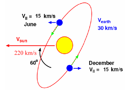
Figure 4: The galactic plane is perpendicular to the paper containing the sun’s velocity. The normal to the two planes form an angle $\gamma^{{}^{\prime}}=\pi/2-\gamma\approx\pi/6$. The modulation is affected by the projection of the Earth’s velocity along the sun’s velocity. Thus the velocity of the detector relative to the center of the galaxy is $220+15=235$ km/s around June 3nd (when the maximum of the event rate is expected) and $220-15=205$ km/s around December 3 (minimum of the event rate).

The LSP velocity distribution f($\upsilon$^′) is not known. Many velocity distributions are employed. In the present work we will adopt the standard practice and assume it to be Gaussian:

$$f(\mbox{\boldmath$\upsilon$}^{\prime})=\frac{1}{(\sqrt{\pi}\mbox{\boldmath$\upsilon_{0}$})^{3}}e^{-(\mbox{\boldmath$\upsilon$}^{\prime}/\mbox{\boldmath$\upsilon_{0}$})^{2}}$$ (79)

Since $\upsilon$${}_{1}\ll$$\upsilon$₀ we will ignore, for the moment, the motion of the Earth. Then the total (non directional) rate is given by

$$R=\bar{R}\,t(a,Q_{min})\,$$ (80)

$$\bar{R}=\frac{\rho(0)}{m_{\chi^{0}}}\frac{m}{Am_{p}}~{}(\frac{\mu_{r}}{\mu_{r}(p)})^{2}~{}\sqrt{\langle v^{2}\rangle}[\sigma_{p,\chi^{0}}^{S}~{}A^{2}+\sigma_{p,\chi^{0}}^{spin}~{}\zeta_{spin}]$$

The SUSY parameters have been absorbed in $\bar{R}$. The parameter $t$ takes care of the nuclear form factor and the folding with LSP velocity distribution Verg00 ; Verg01 ; JDVSPIN04 ; JDV06 . It depends on $Q_{min}$, i.e. the energy transfer cutoff imposed by the detector and $a=[\mu_{r}b\upsilon_{0}\sqrt{2}]^{-1}$.
In the present work we find it convenient to re-write it as:

$$R=\bar{K}\left[c_{coh}(A,\mu_{r}(A))\sigma_{p,\chi^{0}}^{S}+c_{spin}(A,\mu_{r}(A))\sigma_{p,\chi^{0}}^{spin}~{}\zeta_{spin}\right]$$ (81)

where

$$\bar{K}=\frac{\rho(0)}{100\mbox{ GeV}}\frac{m}{m_{p}}~{}\sqrt{\langle v^{2}\rangle}\simeq 160~{}10^{-4}~{}(pb)^{-1}y^{-1}\frac{\rho(0)}{0.3GeVcm^{-3}}\frac{m}{1Kg}\frac{\sqrt{\langle v^{2}\rangle}}{280kms^{-1}}$$ (82)

and

$$c_{coh}(A,\mu_{r}(A))=\frac{100\mbox{ GeV}}{m_{\chi^{0}}}\left[\frac{\mu_{r}(A)}{\mu_{r}(p)}\right]^{2}A~{}t_{coh}(A)$$ (83)

$$c_{spin}(A,\mu_{r}(A))=\frac{100GeV}{m_{\chi^{0}}}\left[\frac{\mu_{r}(A)}{\mu_{r}(p)}\right]^{2}\frac{t_{spin}(A)}{A}$$ (84)

The parameters $c_{coh}(A,\mu_{r}(A))$, $c_{spin}(A,\mu_{r}(A))$, which give the relative merit for the coherent and the spin contributions in the case of a nuclear target compared to those of the proton, have already been tabulated JDV06 for energy cutoff $Q_{min}=0,~{}10$ keV.
Via Eq. (81) we can extract the nucleon cross section from the data (see below).
Neglecting the isoscalar contribution and using $\Omega^{2}_{1}=1.22$ and $\Omega^{2}_{1}=2.8$ for ¹²⁷I and ¹⁹F respectively the extracted nucleon cross sections satisfy:

$$\frac{\sigma^{spin}_{p,\chi^{0}}}{\sigma^{S}_{p,\chi^{0}}}=\left[\frac{c_{coh}(A,\mu_{r}(A))}{c_{spin}(A,\mu_{r}(A))}\right]\frac{3}{\Omega^{2}_{1}}\Rightarrow\approx\times 10^{4}~{}(A=127)~{},~{}\approx\times 10^{2}~{}(A=19)$$ (85)

It is for this reason that the limit on the spin nucleon cross section extracted from both targets is much poorer.

The factors $c19=c_{coh}(19,\mu_{r}(19))$, $s19=c_{spin}(19,\mu_{r}(19))$, $c19=c_{coh}(73,\mu_{r}(73))$, $s73=c_{spin}(73,\mu_{r}(73))$ and $c127=c_{coh}(127,\mu_{r}(127))$, $s127=c_{spin}(127,\mu_{r}(127))$ for two values of $Q_{min}$ and $s3=c_{spin}(3,\mu_{r}(3))$ for $Q_{min}=0$ can be found elsewhere JDV06 .

9 Bounds on the scalar proton cross section

Before proceeding with the analysis of the spin contribution we would like to discuss the limits on the scalar proton cross section. In what follows we will employ for all targets BCFS02 -PAVAN01 the limit of CDMS II for the Ge target CDMSII04 , i.e. $<2.3$ events for an exposure of $52.5$ Kg-d with a threshold of $10$ keV. This event rate is similar to that for other systems SGF05 . The thus obtained limits are exhibited in Fig. 5.

$\sigma_{p}\rightarrow 10^{-5}$pb

$m_{\chi}\rightarrow$ GeV $\sigma_{p}\rightarrow 10^{-5}$pb $m_{\chi}\rightarrow$ GeV

Figure 5: The limits on the scalar proton cross section for A$=127$ on the left and A$=73$ on the right as functions of $m_{\chi}$. The continuous (dashed) curves correspond to $Q_{min}=0~{}(10)$ keV respectively. Note that the advantage of the larger nuclear mass number of the A$=127$ system is counterbalanced by the favorable form factor dependence of the A$=73$ system.

10 Exclusion Plots in the $a_{p},a_{n}$ and $\sigma_{p},\sigma_{n}$ Planes

From the data one can extract a restricted region in the $\sigma_{p},\sigma_{n}$ plane, which depends on the event rate and the LSP mass. Some such exclusion plots have already appeared SGF05 -GIUGIR05 . One can plot the constraint imposed on the quantities $|a_{p}+\frac{\Omega_{n}}{\Omega_{p}}a_{n}|$ and$|\sqrt{\sigma_{p}}+\frac{\Omega_{n}}{\Omega_{p}}\sqrt{\sigma_{n}}e^{i\delta}|^{2}$ derived from the experimental limits via relations:

$$| \sqrt{\sigma_{p}}+\frac{\Omega_{n}}{\Omega_{p}}\sqrt{\sigma_{n}})e^{i\delta}|^{2}\preceq\sigma_{bound}(A)~{}r(m_{\chi},A),$$

$$\sigma_{bound}(A)=\frac{R}{\bar{K}}\frac{3}{\Omega^{2}_{p}}\frac{10^{-5}pb}{c^{100}_{spin}(A,\mu_{r}(A))}~{},~{}r(m_{\chi},A)=\frac{c^{100}_{spin}(A,\mu_{r}(A))}{c_{spin}(A,\mu_{r}(A))}$$

where $\delta$ is the phase difference between the two amplitudes and ${c^{100}_{spin}(A,\mu_{r}(A))}$ is the value of ${c_{spin}(A,\mu_{r}(A))}$ evaluated for the LSP mass of $100$ GeV. Furthermore

$$|a_{p}+\frac{\Omega_{n}}{\Omega_{p}}a_{n}|\preceq a_{bound}(A)~{}\left[r(m_{\chi},A)\right]^{1/2}~{},~{}a_{bound}(A)=\left[\frac{\sigma_{bound}(A)}{3\sigma_{0}}\right]^{1/2}$$ (87)

The constraints will be obtained using the functions ${c^{100}_{spin}(A,\mu_{r}(A))}$, obtained without energy cut off , $Q_{min}=0$, even though the experiments have energy cut offs greater than zero. Furthermore even though we know of no model such that $e^{i\delta}$ is complex, for completeness we will examine below this case as well. Such plots depend on the relative magnitude of the spin matrix elements. They will be given in units of the A-dependent quantity $\sigma_{bound}(A)$ for the nucleon cross sections and the dimensionless quantity $a_{bound}$ for the amplitudes respectively. Before we proceed further we should mention that, if both protons and neutrons contribute, the standard exclusion plot, must be replaced by a sequence of plots, one for each LSP mass or via three dimensional plots. We found it is adequate to provide one such plot for a standard LSP mass, e.g. $100$ GeV, and zero energy threshold. The interested reader can find the scale for any other case in work already published JDV06 . The situation is exhibited in Figs 6-8 in the interesting case of the A=127 system using the nuclear matrix elements of Ressel et al given in Table 2. For other targets we refer to the literature JDV06 .
One can understand the asymmetry in the plot due to the fact that $\Omega_{p}$ is much larger than $\Omega_{n}$. In other words if $\sigma_{p}$ happens to be very small a large $\sigma_{n}$ will be required to accommodate the data. In the example considered here, however, the extreme values differ only by $20\%$ from the values on the axes, which arise, if one assumes that one mechanism at a time (proton or neutron) dominates.

$a_{n}\rightarrow 0.65$

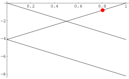
$a_{p}\rightarrow 0.65$ $a_{n}\rightarrow 0.65$ $a_{p}\rightarrow 0.65$

Figure 6: The boundary in the $a_{p},a_{n}$ plane extracted from the data for the target ${}^{127}I$ is shown assuming that the amplitudes are relatively real. The scale depends on the event rate and the LSP mass. Shown here is the scale for $m_{\chi}=100$ GeV. Note that the allowed region is confined when the amplitudes are of the same sign (left plot), but they are not confined when the amplitudes are of opposite sign. The allowed space now is i) The small triangle and ii) The space between the two parallel lines and on the right of the line that intercepts them. We also indicate by a dot the point $a_{p}=-a_{n}$ favored by the spin structure of the nucleon. The nuclear ME employed were those of Ressel and Dean (see table 2)

$\sigma_{n}\rightarrow 5.0\times 10^{-3}$ pb

$\sigma_{n}\rightarrow 5.0\times 10^{-3}$ pb

$\sigma_{p}\rightarrow 5.0\times 10^{-3}$ pb

Figure 7: The same as in Fig. 6 for the $\sigma_{p},\sigma_{n}$ plane. On the left the allowed region is that below the curve (the amplitudes are relatively real and have the same sign) . In the plots on the right the amplitudes are relatively real and of opposite sign. The allowed region is i) between the higher segment of the hyperbola and the straight line and ii) Between the straight line and the lower segment of the curve. The nuclear ME employed were those of Ressel and Dean (see table 2)

$\sigma_{n}\rightarrow 5.0\times 10^{-3}$ pb

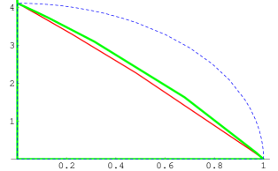
$\sigma_{p}\rightarrow 5.0\times 10^{-3}$ pb

Figure 8: The same as in Fig. 7 assuming that the amplitudes are not relatively real, but are characterized by a phase difference $\delta$. The allowed space is now confined. The results shown for the thin solid, thick solid and dashed curves correspond to $\delta=\pi/3,~{}\pi/6$ and $\pi/2$ respectively .

11 The modulation effect.

As we have mentioned the expected event rate is so low that, even if one goes underground, the background is formidable. Especially since the signal coming from the detection of the energy energy of the recoiling nucleus has the same shape as that of the background. One, therefore, looks for specific signatures associated with the reaction. Since the event rate depends on the relative velocity between the LSP and the target, a periodic seasonal dependence is expected due to the motion of the Earth around the sun. What counts is the the is the projection of the velocity of the earth on the sun’s velocity (see Fig. 4).
If the effects of the motion of the Earth around the sun are included, the total non directional rate is given by

$$R=\bar{K}\left[c_{coh}(A,\mu_{r}(A))\sigma_{p,\chi^{0}}^{S}(1+h(a,Q_{min})cos{\alpha})\right]$$ (88)

and an analogous one for the spin contribution. $h$ is the modulation amplitude, which is quite small, less than $2\%$ and it depends on the velocity distribution, the nuclear form factor and, for a given target, on the LSP mass. $\alpha$ is the phase of the Earth, which is zero around June 2nd. In the case of the target ¹²⁷I the modulation amplitude is shown in Fig. 9.

$h\rightarrow$

$h\rightarrow$

$m_{\chi}\rightarrow$ ($GeV$)

Figure 9: The modulation amplitude $h$ as a function of the LSP mass in the case of ${127}$I for $Q_{min}=0$ on the left and $Q_{min}=10$ keV on the right. We should mention that the average LSP energy for an LSP mass $m_{\chi}=100$ GeV is $\simeq 40$ keV. For the definitions see text.

We see that the modulation amplitude is small, especially for $Q_{min}=0$. Furthermore its sign is uncertain, since it depends on the LSP mass. The modulation amplitude increases as the threshold cut off energy increases, but, unfortunately, this occurs at the expense of the total number of counts. Furthermore many experimentalists worry that there are may be seasonal variations in the relevant backgrounds as well.

12 Transitions to excited states

As we have mentioned the average neutralino energy scales with its mass. It is $\simeq 40$ keV for $m_{\chi}=100$ GeV. Thus the neutralino energy is not high enough to excite the nucleus. In some rare cases involving odd mass nuclei there exist excited states at low energies, which can be populated in the LSP-nucleus collision due to the high velocity tail of the neutralino velocity distribution. From an experimental point of view this is very interesting eji93 , since the signature of the $\gamma-$ray emission following the nuclear de-excitation is much easier than nuclear recoils. An interesting target is ¹²⁷I, which has an excited state at $\simeq 50$ keV. It has recently been found VQS04 that the branching ratio to this excited state is appreciable from an experimental point of view.

BRR$\rightarrow$

BRR$\rightarrow$

$m_{\chi}\rightarrow$ ($GeV$) .

Figure 10: The ratio of the rate to the excited state divided by that of the ground state as a function of the LSP mass (in GeV) for ${}^{127}I$. It was found that the static spin matrix element of the transition from the ground to the excited state is a factor of 1.9 larger than that involving the ground state. The spin response functions $F_{11}(u)$ were assumed to be the same. On the left we show the results for $Q_{min}=0$ and on the right for $Q_{min}=10~{}KeV$. In the last case, due to the detector energy cut, off the denominator (recoil rate) is reduced, while the numerator (the rate to the excited state) is not affected.

13 The directional rates

As we have already mentioned one may attempt to measure not only the energy of the recoiling nucleus, but observe its direction of recoil. Admittedly such experiments are quite hard DRIFT , but they are expected to provide unambiguous signature against background rejection. Since the sun is moving around the galaxy in a directional experiment, i.e. one in which the direction of the recoiling nucleus is observed, one expects a strong correlation of the event rate with the motion of the sun JDVSPIN04 . In fact the directional rate can be written as:

$$R_{dir}=\frac{\kappa}{2\pi}\bar{R}~{}t\,[1+h_{m}cos{(\alpha-\alpha_{m}~{}\pi)}]$$ (89)

where $h_{m}$ is the modulation and $\alpha_{m}$ is the ”shift” in the phase of the Earth $\alpha$, since now the maximum occurs at $\alpha=\alpha_{m}\pi$. $\kappa/(2\pi)$ is the reduction factor of the unmodulated directional rate relative to the non-directional one. The parameters $\kappa~{},~{}h_{m}~{},~{}\alpha_{m}$ depend on the direction of observation:

$$\hat{e}=(\sin{\Theta}\cos{\Phi}~{},~{}\sin{\Theta}\sin{\Phi}~{},~{}\cos{\Theta})$$

The parameter $\kappa t$ for a typical LSP mass $100~{}GeV$ is shown in Fig. 11 as a function of the angle $\Theta$ for the targets $A=19$ and $A=127$. We see that the change of the rate as a function of the angle $\Theta$ for the Maxwellian LSP velocity distribution is quite dramatic. This figure is important in the analysis of the angular correlations, since, among other things, there is always un uncertainty in the determination of the angle in a directional experiment.

$t_{dir}\rightarrow$

$\Theta\rightarrow$ $t_{dir}\rightarrow$ $\Theta\rightarrow$

Figure 11: The quantity $\kappa t$ as a function of the angle $\Theta$, the polar angle from the sun’s direction of motion, for $A=19$ on the left and $A=127$ on the right. The results presented correspond to an LSP mass of $100~{}GeV$.

We prefer to use the parameters $\kappa$ and $h_{m}$, since, being ratios, are expected to be less dependent on the parameters of the theory. We exhibit the dependence of the parameters $t$, $h$, $\kappa,h_{m}$, and $\alpha_{m}$, which are essentially independent of the LSP mass for target $A=19$, in Table 3 (for the other light systems the results are almost identical).

The asymmetry is quite large. For a Gaussian velocity distribution we find:

$$As=\frac{R(-z)-R(+z)}{R(-z)+R(+z)}\approx 0.97$$

In the other directions it depends on the phase of the Earth and is equal to almost twice the modulation. For a heavier nucleus the situation is a bit complicated. Now the parameters $\kappa$ and $h_{m}$ depend on the LSP mass JDVSPIN04 . It is clear that, if such experiments will ever be performed, such signatures cannot be mimicked by background events.

Table 3: The parameters $t$, $h$, $\kappa,h_{m}$ and $\alpha_{m}$ for the isotropic Gaussian velocity distribution and $Q_{min}=0$. The results presented are associated with the spin contribution, but those for the coherent mode are similar. The results shown are for the light systems. For intermediate and heavy nuclei there is a dependence on the LSP mass. $+x$ is radially out of the galaxy ($\Theta=\pi/2,\Phi=0$), $+z$ is in the sun’s direction of motion ($\Theta=0$) and $+y$ is vertical to the plane of the galaxy ($\Theta=\pi/2,\Phi=\pi/2$) so that $(x,y,z)$ is right-handed. $\alpha_{m}=0,1/2,1,3/2$ means that the maximum occurs on the 2nd of June, September, December and March respectively.

type	t	h	dir	$\kappa$	$h_{m}$	$\alpha_{m}$
			+z	0.0068	0.227	1
dir			+(-)x	0.080	0.272	3/2(1/2)
			+(-)y	0.080	0.210	0 (1)
			-z	0.395	0.060	0
all	1.00
all		0.02

14 Observation of electrons produced during the LSP-nucleus collisions

Since the detection of recoiling nuclei is quite hard one may look for other events. One such possibility is the observation of ionization electrons produced directly during the LSP nuclear collisions VE05 , MVE05 . Due to the properties of the bound electron wf, the event rate peaks at very low electron energies. One therefore must be able to achieve very low energy thresholds. In order to avoid uncertainties arising from the constraint SUSY parameter space we have opted to present the ratio of the event rate for producing electrons divided by the standard coherent recoil rate. This ratio is exhibited as a function of the electron threshold energy in Fig. 12. We see that for large atomic number Z and sufficiently low threshold energy this ratio may exceed unity.

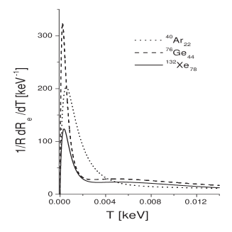
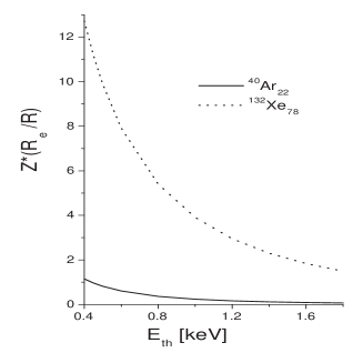
Figure 12: On the left we show the differential rate for ionization electrons, divided by the total rate associated with the nuclear recoils, as a function of the electron energy $T$ (in keV) for various atoms. On the right we show the total rate for producing electrons divided by the corresponding rate for nuclear recoil as a function of the threshold energy. The event rate is per atom, i.e. all electrons in the atom have been considered. The results exhibited were obtained for a typical LSP mass $m_{\chi}=100$ GeV.

.

It has also been found that inner 1s electrons can be ejected with a non negligible probability EMV05 . The produced electron holes can be filled via the Auger process or a sizable fraction can proceed via very hard (32 keV) X-ray emission. The detection of such X-rays, in or without coincidence with nuclear recoils, will provide a signature very hard to miss, if SUSY allows for detectable recoil rates.

15 Conclusions

In this review we have dealt with various issues involving the direct detection of supersymmetric dark matter. The standard experiments employ various techniques of measuring the energy of the recoiling nuclei after their elastic scattering with the dark matter candidates. We have seen that the evaluation of the event rates involves a number of issues: 1) A supersymmetric model with a number of parameters, which at present can only be constrained from laboratory data at low energies as well as cosmological observations. 2) The dependence of the nucleon cross section on quarks other than u and d. 3) A proper nuclear model, which involves the nuclear form factor in the case of the the scalar interaction and the spin response function for the axial current. 4) Information about the density and the velocity distribution of the neutralino (halo model).
Using the present experimental limits on the event rate and suitable inputs in 3)-4) we have derived constraints in the nucleon cross sections. Since the obtained event rates are extremely low, we have examined some additional signatures inherent in the neutralino nucleus interaction, such as the periodic behavior of the rates due to the motion of Earth (modulation effect). Since, unfortunately, this is characterized by a small amplitude, we were lead to examine the possibility of directional experiments. Tese, in addition to the recoil energy, will also attempt to measure the direction of the recoiling nuclei. The event rate in a given direction is $\sim 6\pi$ smaller than that of the standard experiments, but one maybe able to exploit two novel characteristic signatures: a) large asymmetries and b) interesting modulation patterns.
Proceeding further we extended our study to include evaluation of the rates for other than recoil searches such as: i) Transitions to excited states and the observation of de-excitation $\gamma$ rays, ii) detection of the recoiling electrons produced during the neutralino-nucleus collision and iii) observation of hard X-rays, following the de-excitation of the ionized atom.
With all the above signatures one hopes that, if the supersymmetric models do not conspire to lead to large suppression of the amplitudes, the direct direction of dark matter may soon follow.

References

-
(1)
S. Hanary et al: Astrophys. J. 545, L5 (2000);
J.H.P Wu et al: Phys. Rev. Lett. 87, 251303 (2001);
M.G. Santos et al: Phys. Rev. Lett. 88, 241302 (2002). -
(2)
P.D. Mauskopf et al: Astrophys. J. 536, L59 (2002);
S. Mosi et al: Prog. Nuc.Part. Phys. 48, 243 (2002);
S.B. Ruhl al, astro-ph/0212229 and references therein. -
(3)
N.W. Halverson et al: Astrophys. J. 568, 38 (2002)
L.S. Sievers et al: astro-ph/0205287 and references therein. - (4) G. Smoot et al (COBE Collaboration): Astrophys. J. 396, L1 (1992).
- (5) D. Spergel et al: Astrophys. J. Suppl. 148, 175 (2003).
- (6) M. Tegmark et al: Phys.Rev. D 69, 103501 (2004).
- (7) A. Jaffe et al: Phys. Rev. Lett. 86, 3475 (2001).
- (8) G. Jungman, M. Kamionkowski, and K. Griest: Phys. Rep. 267, 195 (1996).
- (9) D. Bennett et al.: Phys. Rev. Lett. 74, 2967 (1995).
- (10) R. Bernabei et al: Phys. Lett. B 389, 757 (1996).
- (11) R. Bernabei et al: Phys. Lett. B 424, 195 (1998).
-
(12)
A. Benoit et al, [EDELWEISS collaboration]: Phys. Lett. B 545, 43
(2002);
V. Sanglar,[EDELWEISS collaboration] arXiv:astro-ph/0306233;
D.S. Akerib et al,[CDMS Collaboration]: Phys. Rev D 68, 082002 (2003); arXiv:astro-ph/0405033. - (13) G. Kane et al: Phys. Rev. D 49, 6173 (1994).
-
(14)
A. Bottino et al., Phys. Lett B 402, 113 (1997).
R. Arnowitt. and P. Nath, Phys. Rev. Lett. 74, 4952 (1995); Phys. Rev. D 54, 2394 (1996); hep-ph/9902237;
V.A. Bednyakov, H.V. Klapdor-Kleingrothaus and S.G. Kovalenko, Phys. Lett. B 329, 5 (1994). - (15) J. Ellis, K. A. Olive, Y. Santoso, and V. C. Spanos: Phys.Rev. D 70, 055005 (2004).
- (16) M. W. Goodman and E. Witten: Phys. Rev. D 31, 3059 (1985).
- (17) P. Ullio and M. Kamioknowski: JHEP 0103, 049 (2001).
-
(18)
M.E.Gómez and J.D. Vergados, Phys. Lett. B 512 , 252 (2001);
hep-ph/0012020.
M.E. Gómez, G. Lazarides and Pallis, C., Phys. Rev.D 61, 123512 (2000) and Phys. Lett. B 487, 313 (2000). - (19) M. Drees and N. N. Nojiri, Phys. Rev. D 48, 3843 (1993); Phys. Rev. D 47, 4226 (1993).
- (20) T.P. Cheng, Phys. Rev. D 38, 2869 (1988); H-Y. Cheng, Phys. Lett. B 219, 347 (1989).
- (21) M.T. Ressell et al., Phys. Rev. D 48, 5519 (1993); M.T. Ressell and D.J. Dean, Phys. Rev. C 56, 535 (1997).
- (22) E. Homlund and M. Kortelainen and T.S. Kosmas and J. Suhonen and J. Toivanen, Phys. Lett B, 584,31 (2004); Phys. Atom. Nucl. 67, 1198 (2004).
-
(23)
A. K. Drukier et al, Phys. Rev. D, 33, 3495 (1986);
J.I. Collar et al., Phys. Lett B 275, 181 (1992). - (24) A. Green: Phys. Rev. D 66, 083003 (2002).
-
(25)
P. Sikivie, I. Tkachev and Y. Wang, Phys. Rev. Let. 75, 2911
(1995); Phys. Rev. D 56, 1863 (1997)
P. Sikivie, Phys. Let. b 432, 139 (1998); astro-ph/9810286. - (26) D. Owen and J. D. Vergados: Astrophys. J. 589, 17 (2003); astro-ph/0203923.
- (27) J.D. Vergados and T.S. Kosmas, Physics of Atomic nuclei, Vol. 61, No 7, 1066 (1998) (from Yadernaya Fisika, Vol. 61, No 7, 1166 (1998).
- (28) K.N. Buckland, M.J. Lehner and G.E. Masek, in Proc. 3nd Int. Conf. on Dark Matter in Astro- and part. Phys. (Dark2000), Ed. H.V. Klapdor-Kleingrothaus, Springer Verlag (2000).
-
(29)
The NAIAD experiment B. Ahmed et al, Astropart. Phys. 19 (2003)
691; hep-ex/0301039
B. Morgan, A. M. Green and N. J. C. Spooner, Phys. Rev. D 71 (2005) 103507; astro-ph/0408047. - (30) H. Ejiri, K. Fushimi, and H. Ohsumi: Phys. Lett. B 317, 14 (1993).
- (31) J. Vergados, P.Quentin, and D. Strottman: IJMPE 14, 751 (2005).
- (32) J. Vergados and H. Ejiri: Phys. Lett. B 606, 305 (2005); hep-ph/0401151.
- (33) C. C. Moustakidis, J. Vergados, and H. Ejiri: Nucl. Phys. B 727, 406 (2005).
- (34) H. Ejiri and Ch.C. Moustakidis and J.D. Vergados, Dark matter search by exclusive studies of X-rays following WIMPs nuclear interactions, (to appear in Phys. Lett.); hep-ph/0507123.
- (35) J. D. Vergados: Part. Nucl. Lett. 106, 74 (2001); hep-ph/0010151.
- (36) K. Griest: Phys. Rev. Lett 61, 666 (1988).
- (37) A. Djouadi and M. K. Drees, Phys. Lett. B 484, 183 (2000); S. Dawson, Nucl. Phys. B 359, 283 (1991); M. Spira it et al, Nucl. Phys. B453, 17 (1995).
- (38) J. Gasser and H. Leutwyler and M.E. Sainio, Phys. Lett. B 253 (1991) 260; ibid B 253 (1991) 260.
- (39) J. Gasser and H. Leutwyler: Phys. Rep. 87, 77 (1982).
- (40) W. B. Kaufmann and G. E. Hite: Phys. Rev. C 60, 055294 (1999).
- (41) M. G. Olsson: Phys. Lett. B 482, 50 (2000); arXiv:hep-ph/0001203.
- (42) M. M. Pavan, I. I. Strakovsky, R. L. Workman, and R. A. Arndt: PiN Newslett. 16, 110 (2002); arXiv:hep-ph/0111066.
- (43) M. G. Olsson and W. B. Kaufmann: PiN Newslett. 16, 382 (2002); arXiv:hep-ph/0111066.
- (44) The Strange Spin of the Nucleon, J. Ellis and M. Karliner, hep-ph/9501280.
- (45) J. D. Vergados: J.Phys. G 30, 1127 (2004).
- (46) P. C. Divari, T. Kosmas, J. D. Vergados, and L. Skouras: Phys. Rev. C 61, 044612 (2000).
- (47) T. Kosmas and J. Vergados: Phys. Rev. D 55, 1752 (1997).
- (48) E. Moulin, F. Mayet, and D. Santos: Phys. Lett. B 614, 143 (2005).
- (49) D. Santos et al, The MIMAC-He3 Collaboration, A New 3He Detector for non Baryonic Dark Matter Search, Invited talk in idm2004 (to appear in the proceedings).
- (50) J. D. Vergados: Phys. Rev. D 62, 023519 (2000).
- (51) J. D. Vergados: Phys. Rev. D 63, 06351 (2001).
- (52) J.D. Vergados, Direct SUSY Dark Matter Detection- Constraints on the Spin Cross Section, hep-ph/0512305.
- (53) P. Belli, R. Cerulli, N. Fornego, and S. Scopel: Phys. Rev. D 66, 043503 (2002); hep-ph/0203242.
- (54) M. M. Pavan, R.A. Arndt, I.I. Strakovsky and R.L. Workman, hep=ph/0111066.
- (55) D. S. Akerib et al (CDMS Collaboration): Phys.Rev.Lett. 93, 211301 (2004).
- (56) C. Savage, P. Gondolo, and K. Freese: Phys. Rev. D 70, 123513 (2004).
- (57) F. Giuliani and T. Girard: Phys.Lett. B 588, 151 (2004).