ZU–TH 02/06

January 2006

Towards $e^{+}e^{-}\to 3$ jets at NNLO by sector decomposition
G. Heinrich
Institut für Theoretische Physik, Universität Zürich, Winterthurerstrasse 190,
CH-8057 Zürich, Switzerland

A method based on sector decomposition has been developed to calculate the double real radiation part of the process $e^{+}e^{-}\to 3$ jets at next-to-next-to-leading order. It is shown in an example that the numerical cancellation of soft and collinear poles works well. The method is flexible to include an arbitrary measurement function in the final Monte Carlo program, such that it allows to obtain differential distributions for different kinds of observables. This is demonstrated by showing 3–, 4– and 5–jet rates at order $\alpha_{s}^{3}$ for a subpart of the process.

1 Introduction

Experiments at LEP have shown that the measurement of jet rates and shape observables in $e^{+}e^{-}$ collisions allow for very stringent tests of the Standard Model, in particular of predictions relying largely on Quantum Chromodynamics (QCD)[1], allowing for example a very precise determination of the strong coupling constant $\alpha_{s}$. A precise knowledge of $\alpha_{s}$ in turn is of major importance at hadron colliders, especially at the LHC. However, the measurements from jets and shapes in $e^{+}e^{-}$ collisions, although being very precise, have not been included in the world average value for $\alpha_{s}$, because it is based only on measurements where next-to-next-to leading order (NNLO) theory predictions are available[2], while for $e^{+}e^{-}\to 3$ jets, full NNLO predictions do not exist yet.

A future International Linear Collider will allow for precision measurements at the per-mille level, which offer the possibility of a determination of $\alpha_{s}$ with unprecedented precision. However, this will only be possible if the theoretical error can keep up with such a precision. As the present error on the NLO prediction for $e^{+}e^{-}\to 3$ jets is dominated by scale uncertainties[3, 4, 5, 6], the calculation of the NNLO corrections to this process will surely lead to an important gain in precision.

After the virtual two-loop corrections entering this calculation have become available[7, 8, 9], the bottleneck now is given by the real radiation part where up to two partons can become theoretically unresolved (soft and/or collinear), leading to infrared singularities upon phase space integration. These singularities have to be subtracted and cancelled with the ones from the virtual contributions before a Monte Carlo program can be constructed. At NNLO, the infrared singularities can be entangled in a complicated way, which renders the extraction of the poles a formidable task. Two different approaches can be followed to achieve this task:

1. Construction of a subtraction scheme where the subtraction terms are integrated analytically in $D=4-2\epsilon$ dimensions over the unresolved phase space, thus extracting the poles in $1/\epsilon$. The main advantages of this approach are the following: It allows maximal (i.e. analytical) control over the pole terms, and it insures a minimal number of subtraction terms, as the latter are constructed manually by considering all physical situations where a singular configuration is approached. The drawbacks of this method are given by the fact that constructing such a scheme is a highly non-trivial and tedious task, especially in view of the fact that it is different for each colour structure. Further, the analytic integration over subtraction terms may become impossible when applying the method to other processes where several mass scales are involved.

2. Sector decomposition, where the poles are isolated by an automated routine and the pole coefficients are integrated numerically. The advantages of this approach reside in the fact that the extraction of the infrared poles is algorithmic, being the same for all colour factors, and that the subtraction terms can be arbitrarily complicated as they are integrated only numerically. On the other hand, the algorithm which isolates the poles increases the number of original functions and in general does not lead to the minimal number of subtraction terms, thus producing rather large expressions.

Approach 1. has been pursued by several groups in different variations[10, 11, 12, 13, 14, 15, 16, 17, 18, 19, 20, 21, 22, 23], and the implementation of the method based on antenna subtraction[19, 23] into a Monte Carlo program is presently underway[24]. The sector decomposition approach has seen a very rapid development recently. Sector decomposition is a general method to disentangle overlapping singularities in parameter space, originally used by K. Hepp[25] for overlapping ultraviolet singularities. It has been very successfully applied to various types of multi-loop integrals since[26, 27, 28, 29, 30, 31, 32]. Its application to NNLO phase space integrals, first proposed in[33], already lead to a number of promising results  [15, 34, 35, 36, 37, 32].

The present paper deals with the application of sector decomposition to the double real radiation part of the process $e^{+}e^{-}\to 3$ jets at NNLO, which involves subprocesses of the type $\gamma^{*}\to 5$ partons. The matrix elements for the processes $\gamma^{*}\to q\bar{q}ggg$ and $\gamma^{*}\to q\bar{q}q^{\prime}\bar{q}^{\prime}g$ are huge, such that the calculation also involves non-trivial book-keeping and file handling tasks, which are not addressed in this article. The intention of this paper is to show that a method has been developed which can deal with $1\to 5$ parton processes efficiently, such that the construction of a fully differential Monte Carlo program for the process $e^{+}e^{-}\to 3$ jets at NNLO is merely a matter of putting pieces together, which will be left to a future publication. Therefore, we only consider one sample topology (including the full tensor structure) as part of the full matrix element. For this topology, we first calculate the fully inclusive integral over the 5-parton phase space, leading to poles up to $1/\epsilon^{4}$. In order to prove the correctness of the result, we also calculate all possible cuts of this diagram with less than five particles in the final state. For the contribution from $\gamma^{*}\to 4$ partons, we use the result obtained in [35] by sector decomposition. The KLN theorem[38, 39] guarantees that the sum of all possible cuts of the UV renormalised diagram is finite. This is demonstrated in section 2. However, the method is not limited to calculate only inclusive cross sections. As the singularities are disentangled by an algebraic algorithm, the inclusion of an arbitrary (infrared safe) measurement function – at the stage of the numerical evaluation of the finite functions produced by sector decomposition – does not present a problem. This is shown in section 3. As an illustration of the action of the measurement function, the ${\cal O}(\alpha_{s}^{3})$ 3–, 4– and 5–jet rates are shown for the sample matrix element as a function of the cut parameter $y^{\rm cut}$ within the JADE algorithm[40]. Section 4 contains the conclusions. Details of the calculation are given in appendix A.

2 Cancellation of Divergences

As explained above, the method presented here addresses the main difficulty in calculating the real radiation part of $e^{+}e^{-}\to 3$ jets at NNLO, which is the isolation and subtraction of the infrared poles which occur when integrating the squared amplitude over the phase space for $\gamma^{*}\to 5$ partons.

In order to check the correctness of the results for the integrals over the $1\to 5$ particle phase space, one can exploit the fact that the sum over all cuts of a given (UV renormalised) topology must be infrared finite. In order to demonstrate these cancellations, let us consider as an example the diagram depicted in Fig. 1, occurring in the part $\sim C_{F}^{3}$ of the squared amplitude for $e^{+}e^{-}\to 3$ jets at NNLO.

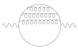
Figure 1: The ladder diagram

Summing over all cuts of this diagram and performing UV renormalisation, we obtain the condition

$$T_{1\to 5}+z_{1}\,T_{1\to 4}+z_{2}\,T_{1\to 3}+z_{3}\,T_{1\to 2} = \mbox{finite}\;,$$ (2.1)

where $T_{1\to i}$ denotes the diagram with $i$ cut lines as shown in Figure 2.

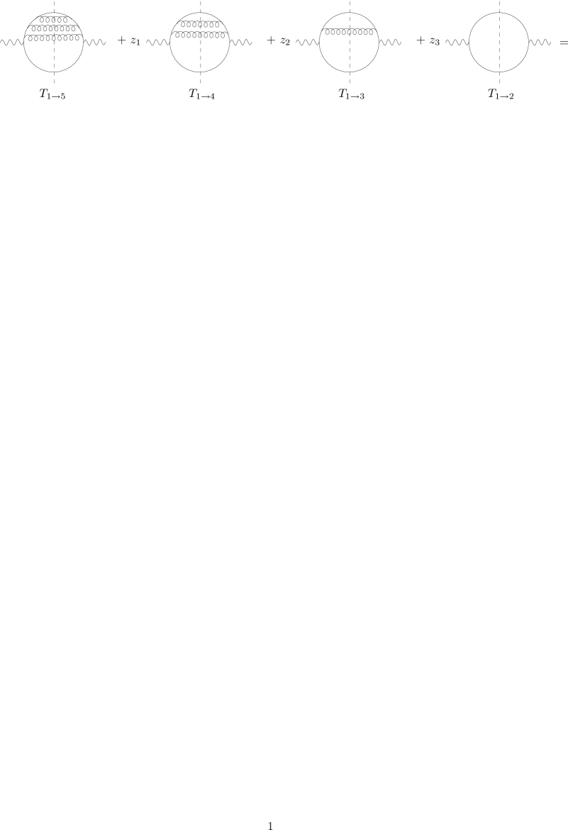
Figure 2: Cancellation of IR divergences in the sum over all cuts of the renormalised graph

2.1 UV renormalisation

For $i=1,2$, the renormalisation constants $z_{i}$ (in Feynman gauge) already have been calculated in [35], to be given by

$$z_{1} = C_{F}\frac{\alpha_{s}}{4\pi}\,\frac{1}{\epsilon}$$ (2.2)

$$z_{2} = C_{F}^{2}\left(\frac{\alpha_{s}}{4\pi}\right)^{2}\,\left(\frac{1}{2\epsilon^{2}}-\frac{1}{4\epsilon}\right)$$ (2.3)

The 3-loop renormalisation constant $z_{3}$ will be derived in the following. Using the graphical BHPZ notation as in ref.[35], 3-loop renormalisation of the fermion selfenergy implies that the combination of graphs as shown in Fig. 3 is finite.

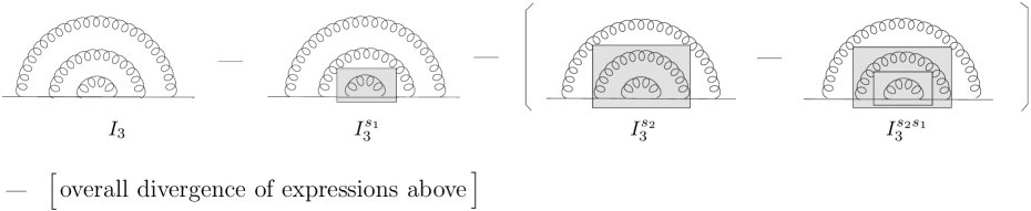
Figure 3: UV renormalisation of the quark propagator at ${\cal O}(\alpha_{s}^{3})$

The explicit calculation yields:

$$I_{3} = i\not p\,C_{F}^{3}\left(\frac{\alpha_{s}}{4\pi}\right)^{3}\,\left(\frac{-p^{2}}{\mu^{2}}\right)^{-3\epsilon}\frac{4(1-\epsilon)^{3}}{\Gamma^{3}(1+\epsilon)}\,G(1,1,0)G(1+2\epsilon,1,1)$$ (2.4)

$$\times \Bigl{\{}G(\epsilon,1,0)+G(1+\epsilon,1,0)-G(1+\epsilon,1,1)\Bigr{\}}$$

$$G(\alpha,\beta,n) = \frac{\Gamma(\alpha+\beta-D/2)}{\Gamma(\alpha)\Gamma(\beta)}\,\frac{\Gamma(D/2-\alpha+n)\,\Gamma(D/2-\beta)}{\Gamma(D-\alpha-\beta+n)}\quad,\quad D=4-2\epsilon$$

$$I_{3}^{s_{1}} = i\not p\,C_{F}^{3}\left(\frac{\alpha_{s}}{4\pi}\right)^{3}\,\left(\frac{-p^{2}}{\mu^{2}}\right)^{-2\epsilon}\frac{(1-\epsilon)^{2}\Gamma^{3}(1-\epsilon)\Gamma(1+2\epsilon)}{\epsilon^{3}\Gamma^{2}(1+\epsilon)\Gamma(3-3\epsilon)}$$ (2.5)

$$I_{3}^{s_{2}} = i\not p\,C_{F}^{3}\left(\frac{\alpha_{s}}{4\pi}\right)^{3}\,\left(\frac{-p^{2}}{\mu^{2}}\right)^{-\epsilon}\frac{(1-\epsilon)\Gamma^{2}(1-\epsilon)}{\epsilon^{3}\Gamma(2-2\epsilon)}\left\{\frac{1}{2}+\frac{5}{4}\epsilon-\epsilon\log{(-p^{2}/\mu^{2})}\right\}$$ (2.6)

$$I_{3}^{s_{2}s_{1}} = i\not p\,C_{F}^{3}\left(\frac{\alpha_{s}}{4\pi}\right)^{3}\,\left(\frac{-p^{2}}{\mu^{2}}\right)^{-\epsilon}\frac{(1-\epsilon)\Gamma^{2}(1-\epsilon)}{\epsilon^{3}\Gamma(2-2\epsilon)}\left\{1+\epsilon-\epsilon\log{(-p^{2}/\mu^{2})}\right\}$$ (2.7)

The overall divergences $J^{s_{i}}_{3}=$ overall div $[I^{s_{i}}_{3}]$ of the diagrams above are thus given by

$$J_{3} = i\not p\,C_{F}^{3}\left(\frac{\alpha_{s}}{4\pi}\right)^{3}\,\Bigl{\{}\frac{1}{6\epsilon^{3}}+\frac{3}{4\epsilon^{2}}-\frac{1}{2\epsilon^{2}}\log{(-p^{2}/\mu^{2})}$$ (2.8)

$$+\frac{1}{\epsilon}\,[\frac{79}{24}-\frac{\pi^{2}}{2}-\frac{9}{4}\log{(-p^{2}/\mu^{2})}+\frac{3}{4}\log^{2}{(-p^{2}/\mu^{2})}]\Bigr{\}}$$

$$J_{3}^{s_{1}} = i\not p\,C_{F}^{3}\left(\frac{\alpha_{s}}{4\pi}\right)^{3}\,\Bigl{\{}\frac{1}{2\epsilon^{3}}+\frac{5}{4\epsilon^{2}}-\frac{1}{\epsilon^{2}}\log{(-p^{2}/\mu^{2})}$$ (2.9)

$$+\frac{1}{\epsilon}\,[\frac{31}{8}-\frac{\pi^{2}}{6}-\frac{5}{2}\log{(-p^{2}/\mu^{2})}+\log^{2}{(-p^{2}/\mu^{2})}]\Bigr{\}}$$

$$J_{3}^{s_{2}} = i\not p\,C_{F}^{3}\left(\frac{\alpha_{s}}{4\pi}\right)^{3}\,\Bigl{\{}\frac{1}{2\epsilon^{3}}+\frac{7}{4\epsilon^{2}}-\frac{3}{2\epsilon^{2}}\log{(-p^{2}/\mu^{2})}$$ (2.10)

$$+\frac{1}{\epsilon}\,[\frac{9}{4}-\frac{\pi^{2}}{12}-\frac{3}{2}\log{(-p^{2}/\mu^{2})}+\frac{5}{4}\log^{2}{(-p^{2}/\mu^{2})}]\Bigr{\}}$$

$$J_{3}^{s_{2}s_{1}} = i\not p\,C_{F}^{3}\left(\frac{\alpha_{s}}{4\pi}\right)^{3}\,\Bigl{\{}\frac{1}{\epsilon^{3}}+\frac{2}{\epsilon^{2}}-\frac{2}{\epsilon^{2}}\log{(-p^{2}/\mu^{2})}$$ (2.11)

$$+\frac{1}{\epsilon}\,[3-\frac{\pi^{2}}{6}-3\log{(-p^{2}/\mu^{2})}+\frac{3}{2}\log^{2}{(-p^{2}/\mu^{2})}]\Bigr{\}}\;.$$

Note that we have adopted the $\overline{\rm{MS}}$ prescription

$$\alpha=C_{\overline{\rm{MS}}}\,\alpha^{0},\alpha_{s}=C_{\overline{\rm{MS}}}\,\alpha_{s}^{0}\,,\;C_{\overline{\rm{MS}}}=\Gamma(1+\epsilon)\,\left(\frac{4\pi}{\mu^{2}}\right)^{\epsilon}\;.$$

From eqs. (2.8) to (2.11) we can now derive $z_{3}$ as

$$i\not p\,z_{3} = J_{3}-J_{3}^{s_{1}}-(J_{3}^{s_{2}}-J_{3}^{s_{2}s_{1}})$$

$$\Rightarrow z_{3} = C_{F}^{3}\left(\frac{\alpha_{s}}{4\pi}\right)^{3}\,\left(\frac{1}{6\epsilon^{3}}-\frac{1}{4\epsilon^{2}}+\frac{1}{6\epsilon}\right)\;.$$ (2.12)

The non-local logarithmic terms cancel, as guaranteed by the BHPZ theorem[41, 25, 42].

2.2 Combining the renormalised diagrams

In order to verify eq. (2.1), we have to integrate the ladder diagrams corresponding to the process $\gamma^{*}\to i$ partons over the $1\to i$ particle phase space. Up to $i=4$, this has been done already in ref.[35], where $T_{1\to 4}$ has been calculated by sector decomposition. The important new ingredient here is the calculation of $T_{1\to 5}$. Before showing this calculation in more detail, let us first construct the expressions entering eq. (2.1) for $i<5$. From ref.[35], we have

$$T_{1\to 2} = 2\,\alpha\,q^{2}\,\left(\frac{q^{2}}{\mu^{2}}\right)^{-\epsilon}\,\frac{(1-\epsilon)\Gamma(1-\epsilon)}{\Gamma(1+\epsilon)\Gamma(2-2\epsilon)}$$ (2.13)

$$T_{1\to 3} = -z_{1}\,T_{1\to 2}\,\left(\frac{q^{2}}{\mu^{2}}\right)^{-\epsilon}\frac{2\,(1-\epsilon)^{2}\Gamma(1-\epsilon)^{2}}{\Gamma(1+\epsilon)\Gamma(3-3\epsilon)}$$ (2.14)

$$T_{1\to 4} = (\epsilon\,z_{1})^{2}\,T_{1\to 2}\,\left(\frac{q^{2}}{\mu^{2}}\right)^{-2\epsilon}\frac{1}{\Gamma(1+\epsilon)^{2}\Gamma(1-2\epsilon)}\,\left\{\frac{1}{2\epsilon^{2}}+\frac{11}{4\epsilon}+7.869\right\}$$ (2.15)

Combination of these results with the renormalisation constants given in section 2.1 leads to

$$z_{1}\,T_{1\to 4}+z_{2}\,T_{1\to 3}+z_{3}\,T_{1\to 2}=$$ (2.16)

$$C_{F}^{3}\left(\frac{\alpha_{s}}{4\pi}\right)^{3}\,T_{1\to 2}\left\{\frac{1}{6\epsilon^{3}}+\frac{1}{2\epsilon^{2}}\,[3-\log{\left(\frac{q^{2}}{\mu^{2}}\right)}]+\frac{1}{\epsilon}\,[5.608-\frac{9}{2}\log{\left(\frac{q^{2}}{\mu^{2}}\right)]+\frac{3}{4}\log^{2}{\left(\frac{q^{2}}{\mu^{2}}\right)}}\,+\,\mbox{finite}\right\}$$

What remains to be shown now is that the 5-parton contribution $T_{1\to 5}$ exactly cancels the poles in (2.16).

2.3 Calculation of the 5-particle contribution

The graph $T_{1\to 5}$ is calculated numerically by sector decomposition. To this aim, the phase space integrals are brought to a form where all integrations are from zero to one, as described in more detail in appendix A. Note that the parametrisation given here is particularly convenient for the denominator structure of our sample topology. In order to deal with the full matrix element, several parametrisations have been worked out, each one optimised to be applied to a certain class of denominators. An automated subroutine scans the denominators of a given matrix element and applies the appropriate parametrisation. In this way, the full expression naturally is split into tractable subparts.

After having performed the transformations of the phase space integration variables as explained in appendix A.1, the $1\to 5$ phase space in $D$ dimensions is given by eq.(A.7):

$$\int d\Phi_{1\to 5}^{D} = {\cal K}^{(5)}_{\Gamma}(q^{2})^{2D-5}\int_{0}^{1}\prod\limits_{i=2}^{10}dt_{i}\,[t_{5}(1-t_{5})]^{-1-\epsilon}[t_{8}(1-t_{8})t_{10}(1-t_{10})]^{-\frac{1}{2}-\epsilon}$$ (2.17)

$$[t_{2}\,t_{6}(1-t_{6})(1-t_{7})]^{1-2\epsilon}[(1-t_{2})t_{3}(1-t_{3})t_{4}(1-t_{4})t_{9}(1-t_{9})]^{-\epsilon}\,t_{7}^{2-3\epsilon}$$

$${\cal K}^{(5)}_{\Gamma} = \frac{2\pi^{4\epsilon}}{(4\pi)^{9}\Gamma(-2\epsilon)\Gamma(2-2\epsilon)}\;.$$

Singularities only occur at the boundaries $t_{i}=0,1$. Further, one can split the integrations at $t_{i}=1/2$ and remap the variables to the unit cube to assure that all potential singularities occur only for $t_{i}\to 0$. However, as this procedure doubles the number of integrals for each $t_{i}$, it is only done for those variables where a singularity at $t_{i}=1$ is possible at all, in order to avoid a proliferation of terms.

The matrix element typically contains terms of the structure

$$I = \int_{0}^{1}dx\int_{0}^{1}dy\,x^{-1-\epsilon}\,(x+y)^{-1}\;,$$

where a naive subtraction of the singularity for $x\to 0$ of the form

$$\int_{0}^{1}dx\int_{0}^{1}dy\,x^{-1-\epsilon}f(x,y) = -\frac{1}{\epsilon}\int_{0}^{1}dy\,\ f(0,y)+\int_{0}^{1}dx\int_{0}^{1}dy\,x^{-\epsilon}\,\frac{f(x,y)-f(0,y)}{x}$$

fails, because the singularities for $x\to 0$ and $y\to 0$ are overlapping. This is where sector decomposition shows its virtues. The working mechanism of sector decomposition already has been explained in detail in[27] and therefore will be outlined only shortly here. The basic idea is to first split the integration region into sectors where the variables $x$ and $y$ are ordered.

$$I=\int_{0}^{1}dx\int_{0}^{1}dy\,x^{-1-\epsilon}\,(x+y)^{-1}\,[\underbrace{\Theta(x-y)}_{(1)}+\underbrace{\Theta(y-x)}_{(2)}]$$

Then remapping the integration domain to the unit cube, the singularities in our simple example are already disentangled: After the substitutions $y=x\,t$ in sector (1) and $x=y\,t$ in sector (2), one has

$$I = \int_{0}^{1}dx\,x^{-1-\epsilon}\int_{0}^{1}dt\,(1+t)^{-1}+\int_{0}^{1}dy\,y^{-1-\epsilon}\int_{0}^{1}dt\,t^{-1-\epsilon}\,(1+t)^{-1}\;.$$

For more complicated functions, several iterations of this procedure may be necessary, but it is easily implemented into an automated subroutine. Once all singularities are factored out, the result can be expanded in $\epsilon$, where the subtraction of the pole terms naturally leads to plus distributions by the identity

$$x^{-1+\kappa\epsilon}=\frac{1}{\kappa\,\epsilon}\,\delta(x)+\sum_{n=0}^{\infty}\frac{(\kappa\epsilon)^{n}}{n!}\,\left[\frac{\ln^{n}(x)}{x}\right]_{+}\;\mbox{ where }\int_{0}^{1}dx\,\left[f(x)/x\right]_{+}=\int_{0}^{1}dx\,\frac{f(x)-f(0)}{x}\;.$$

In this way, a Laurent series in $\epsilon$ is obtained, where the pole coefficients are sums of finite parameter integrals which can be evaluated numerically.

Note that the numerator structure of the matrix element can only improve the infrared pole structure, such that it can be included later, at the stage of the expansion in $\epsilon$. It also should be mentioned that for some phase space parametrisations, required to tackle the full matrix element, square-root terms in the denominator are unavoidable. Such terms can spoil the simple scaling behaviour which is crucial for the algorithm to work. However, one can always find (nonlinear) variable transformations such that these terms can be mapped to a form which is amenable to sector decomposition.

Applying the method to our sample diagram, and requiring a numerical precision of 1%, the following result is obtained after an integration time of about 20 minutes on a 2.8 GHz Pentium IV PC:

$$T_{1\to 5} = -C_{F}^{3}\left(\frac{\alpha_{s}}{4\pi}\right)^{3}\,T_{1\to 2}\left\{\frac{0.16662}{\epsilon^{3}}+\frac{1}{\epsilon^{2}}\,[1.4993-0.4999\,\log{\left(\frac{q^{2}}{\mu^{2}}\right)}]\right.$$ (2.18)

$$\left.+\frac{1}{\epsilon}\,[5.5959-4.4978\,\log{\left(\frac{q^{2}}{\mu^{2}}\right)}+0.74978\,\log^{2}{\left(\frac{q^{2}}{\mu^{2}}\right)}]\,+\,\mbox{finite}\right\}\;.$$

Combining eqs. (2.16) and (2.18) we see that all poles cancel within the numerical precision.

3 Inclusion of a measurement function

The isolation of infrared poles by sector decomposition is an algebraic procedure, leading to a set of finite functions for each pole coefficient as well as for the finite part. The finite part can be written to a Monte Carlo program and combined with any infrared safe measurement function. To this aim, one has to take the limit $D\to 4$ of the $D$-dimensional phase space, which is non-trivial because in $D=4$, the Gram determinant of five light-like momenta vanishes, which means that only 8 Mandelstam invariants are independent, whereas in $D=4-2\epsilon$ one has 9 independent invariants, i.e. 9 independent phase space integration variables, and sector decomposition acts in $D=4-2\epsilon$ dimensions. How this problem is solved is explained in appendix A.2. It is also described there how the four-momenta of the particles in the final state in terms of energies and angles are reconstructed from the phase space integration variables $t_{i}$. Note that the variables $t_{i}$ are transformed in the course of sector decomposition, such that for each function which is an endpoint of the sector decomposition tree, the expressions for the invariants $s_{ij}$ in terms of the final Monte Carlo integration variables look different. This requires careful (automated) book-keeping, but does not constitute a principal problem.

Further, it has to be assured that the subtraction terms only come to action in phase space regions which are allowed by the measurement function. To illustrate this point, consider the simple one-dimensional example where the measurement function is just a step function $\Theta(x-a),\,a>0$, and the “matrix element” after sector decomposition is given by a plus distribution $[f(x)/x]_{+}$. If we naively combine the plus distribution with our measurement function, we obtain

$$\int_{0}^{1}\,dx\,\frac{f(x)-f(0)}{x}\,\Theta(x-a)=f(0)\,\ln{a}+\int_{a}^{1}\,dx\,\frac{f(x)}{x}\;.$$ (3.1)

On the other hand, the $f(0)$ term stems from the subtraction of a singularity at $x=0$, which is now killed by our measurement function anyway, such that inclusion of the $f(0)$ term would lead to a wrong result. Therefore, the correct way to include the measurement function is of course

$$\int_{0}^{1}dx\,\frac{f(x)\Theta(x-a)-f(0)\Theta(-a)}{x}\;.$$ (3.2)

However, this does not mean that the $\epsilon$–expansions and subtractions have to be redone each time the measurement function is changed. It can be achieved by including symbolic functions in the $\epsilon$–expansion which, depending on the generated phase space point in the Monte Carlo program, take on the appropriate values.

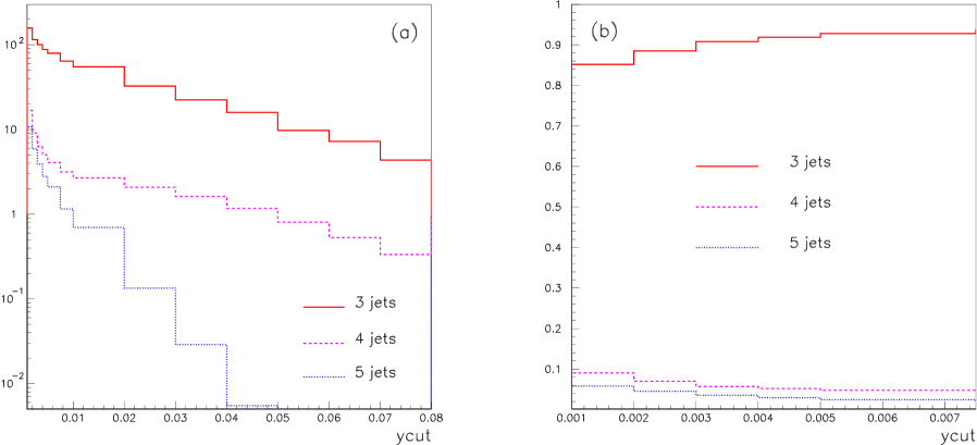
Figure 4: 3–, 4– and 5–jet rates at order $\alpha_{s}^{3}$ for the sample matrix element

As an example, the JADE algorithm[40] to define 3–, 4– and 5–jet events has been implemented into a Monte Carlo program built upon the output of sector decomposition, using the multi-dimensional integration package BASES[43]. For the plots in Figs. 4a and 4b, the diagram discussed in this paper (summed over all cuts) served as a toy matrix element, but it should be emphasised that the same Monte Carlo program can be used to calculate the full process $e^{+}e^{-}\to 3,4,5$ jets at order $\alpha_{s}^{3}$, once the contributions from the other topologies are implemented. Further, the architecture of the program is such that the JADE algorithm can be easily replaced by a different jet algorithm, and shape observables can also be defined.

Figures 4a and 4b show the 3–, 4– and 5–jet rates at order $\alpha_{s}^{3}$, as a function of the jet separation parameter $y^{\rm cut}$. In Figure 4a, the y-axis is in arbitrary units, whereas in Figure 4b the rates are normalised to the sum of the 3–, 4– and 5–jet rates. The renormalisation scale $\mu^{2}$ has been set equal to $q^{2}$, the center of mass energy of the $e^{+}e^{-}$ system. As in the previous section, the numerical precision is 1%. Figure 4a shows that the 5–jet rate drops drastically as $y^{\rm cut}$ increases, as to be expected. The 3-jet rate decreases only slowly, as only few events are classified as 2–jet events and thus rejected for values of $y^{\rm cut}\leq 0.08.$ Figure 4b demonstrates how the 3-jet rate decreases in favour of the 4– and 5–jet rates if $y^{\rm cut}$ becomes very small.

4 Conclusions and Outlook

In this paper, a method based on sector decomposition to calculate the double real radiation part of the process $e^{+}e^{-}\to 3$  jets at ${\cal O}(\alpha_{s}^{3})$ has been presented. The sector decomposition algorithm serves to isolate, by an automated algebraic subroutine, the infrared poles which occur upon phase space integration if one or several particles in the final state become soft and/or collinear. In this way, one is dispensed from the manual construction of a subtraction scheme. The cancellation of the poles is shown by numerical calculation of the pole coefficients.

For the process $e^{+}e^{-}\to 3$  jets at NNLO, integration over a phase space with up to five particles in the final state is necessary, where up to two particles can become soft and collinear. It has been proven that the program handles the isolation and subtraction of the poles correctly by considering all possible cuts of a specific diagram which is a subpart of the colour structure $\sim C_{F}^{3}$ contained in the full matrix element at order $\alpha_{s}^{3}$. Summing over all the cuts, the poles cancel within the numerical precision.

The finite part has been implemented into a Monte Carlo program which allows the inclusion of a measurement function in order to obtain differential distributions for arbitrary (infrared safe) observables. As an example, the 3–, 4– and 5–jet rates at order $\alpha_{s}^{3}$ as a function of the jet separation parameter $y^{\rm cut}$ are shown for the subpart of the full matrix element treated in this paper. As this toy matrix element already shows most of the problems which occur in the double real radiation part, while the one-loop virtual corrections combined with the $1\to 4$ phase space, as well as the two-loop virtual part combined with the $1\to 3$ phase space, are relatively easy (because the virtual integrals only lead to renormalisation factors), it is an ideal testing ground for the method presented here to tackle massless $1\to 5$ processes. For the calculation of the full matrix element, the expressions to be integrated numerically in the double real radiation part will of course be much larger, but the method described in this paper can handle them in the same way. The virtual corrections will also be more complicated, but can be treated with sector decomposition applied to loop integrals[27], for the kinematics of $e^{+}e^{-}$ annihilation. Therefore the problem is basically reduced to large file handling, book-keeping and implementation time/CPU time.

For the parts of the full matrix element considered so far, the numerical stability is very good. A reason might be that the subtractions within the sector decomposition method are local in the sense of plus distributions, i.e. the singular limits in each integration variable are directly subtracted.

CPU time will become an issue for the treatment of the full process, but as the method relies on a division of the amplitude squared into different “topologies” corresponding to different classes of denominator structures, the problem is naturally split into smaller subparts. If such a “trivial parallelisation” is not sufficient, there is still the possibility to parallelise the evaluation of the functions produced by sector decomposition.

As the method is based on a universal algorithm acting on integration variables, and does not require analytic integration over complicated functions, it will surely see a number of interesting applications in the future, in particular in what concerns the production of massive particles.

Appendix A Massless 5-parton Phase Space

A.1 Phase space $1\to 5$ in $D\not=4$ dimensions

The phase space for the decay of one off-shell particle with momentum $q$ into $N$ massless particles with momenta $p_{1},\ldots,p_{N}$ in $D$ dimensions is given by

$$\int d\Phi_{1\to N}^{D} = (2\pi)^{N-D(N-1)}\int\prod\limits_{j=1}^{N}d^{D}p_{j}\,\delta^{+}(p_{j}^{2})\delta\Bigl{(}q-\sum\limits_{i=1}^{N}p_{i}\Bigr{)}$$ (A.1)

$$= (2\pi)^{N-D(N-1)}\,2^{1-N}\int\prod\limits_{j=1}^{N-1}d^{D-1}\vec{p}_{j}\,\frac{\Theta(E_{j})}{E_{j}}\,\delta^{+}([q-\sum\limits_{i=1}^{N-1}p_{i}]^{2})\;.$$

For $N=5$, we parametrise the momenta in $D$ dimensions as (ordering of the vector components:
$(E,(D-4),x,y,z)$)

$$q = (q,\vec{0}^{(D-1)})$$

$$p_{1} = E_{1}\,(1,\vec{0}^{(D-2)},1)$$

$$p_{2} = E_{2}\,(1,\vec{0}^{(D-3)},\sin\theta_{1},\cos\theta_{1})$$

$$p_{3} = E_{3}\,(1,\vec{0}^{(D-4)},\sin\theta_{2}\sin\theta_{4},\sin\theta_{2}\cos\theta_{4},\cos\theta_{2})$$

$$p_{4} = E_{4}\,(1,(\vec{0}^{(D-5)},\sin\theta_{6}\sin\theta_{5}\sin\theta_{3}),\cos\theta_{6}\sin\theta_{5}\sin\theta_{3},\cos\theta_{5}\sin\theta_{3},\cos\theta_{3})$$

$$p_{5} = q-p_{1}-p_{2}-p_{3}-p_{4}$$ (A.2)

Inserting this parametrisation into (A.1) and carrying out integrations over azimuthal angles leads to

$$\int d\Phi_{1\to 5}^{D} = (2\pi)^{5-4D}2^{-4}V(D-1)V(D-2)V(D-3)V(D-4)$$ (A.3)

$$\int\prod\limits_{j=1}^{4}dE_{j}\,\Theta(E_{j})\,d\theta_{1}\ldots d\theta_{6}\left[E_{1}E_{2}E_{3}E_{4}\sin\theta_{1}\sin\theta_{2}\sin\theta_{3}\right]^{D-3}$$

$$\left[\sin\theta_{4}\sin\theta_{5}\right]^{D-4}(\sin\theta_{6})^{D-5}\,\delta^{+}([q-\sum\limits_{i=1}^{4}p_{i}]^{2})$$

$$\mbox{where }\,V(D) = 2\pi^{\frac{D}{2}}/\Gamma(\frac{D}{2})\;.$$

Introducing the scaled invariants $y_{i}$ as new integration variables

$$y_{1}=s_{12}/q^{2},y_{2}=s_{13}/q^{2},y_{3}=s_{23}/q^{2},y_{4}=s_{14}/q^{2},y_{5}=s_{24}/q^{2},$$

$$y_{6}=s_{34}/q^{2},y_{7}=s_{15}/q^{2},y_{8}=s_{25}/q^{2},y_{9}=s_{35}/q^{2},y_{10}=s_{45}/q^{2}$$

leads to the Jacobian

$$|\det J| = 2^{10}q^{4}\left[E_{1}E_{2}E_{3}E_{4}\sin\theta_{1}\sin\theta_{2}\sin\theta_{3}\right]^{3}\left[\sin\theta_{4}\sin\theta_{5}\right]^{2}\sin\theta_{6}\;.$$

The Jacobian can be expressed in terms of the determinant of the Gram matrix $G_{ij}=2p_{i}\cdot p_{j}$

$$\det G = -2^{5}q^{2}\left[E_{1}E_{2}E_{3}E_{4}\sin\theta_{1}\sin\theta_{2}\sin\theta_{3}\sin\theta_{4}\sin\theta_{5}\sin\theta_{6}\right]^{2}$$

$$\Rightarrow|\det J| = \sqrt{2^{15}q^{6}\,(-\det G)}\,\left[E_{1}E_{2}E_{3}E_{4}\sin\theta_{1}\sin\theta_{2}\sin\theta_{3}\right]^{2}\sin\theta_{4}\sin\theta_{5}\;.$$

After these variable transformations, the phase space is given by

$$\int d\Phi_{1\to 5}^{D} = (2\pi)^{5-4D}2^{-2-2D}V(D-1)V(D-2)V(D-3)V(D-4)(q^{2})^{2D-5}$$ (A.4)

$$\int\prod\limits_{j=1}^{10}dy_{j}\,\delta(1-\sum\limits_{i=1}^{10}y_{i})\,(-\Delta_{5})^{\frac{D}{2}-3}\Theta(-\Delta_{5})$$

where

$$-\Delta_{5} = y_{10}^{2}y_{1}y_{2}y_{3}+y_{9}^{2}y_{1}y_{4}y_{5}+y_{8}^{2}y_{2}y_{4}y_{6}+y_{7}^{2}y_{3}y_{5}y_{6}+y_{6}^{2}y_{1}y_{7}y_{8}$$ (A.5)

$$+y_{5}^{2}y_{2}y_{7}y_{9}+y_{4}^{2}y_{3}y_{8}y_{9}+y_{3}^{2}y_{4}y_{7}y_{10}+y_{2}^{2}y_{5}y_{8}y_{10}+y_{1}^{2}y_{6}y_{9}y_{10}$$

$$+y_{10}\,[y_{2}y_{3}y_{5}y_{7}+y_{1}y_{3}y_{6}y_{7}+y_{2}y_{3}y_{4}y_{8}+y_{1}y_{2}y_{6}y_{8}+y_{1}y_{3}y_{4}y_{9}+y_{1}y_{2}y_{5}y_{9}]$$

$$+y_{9}\,[y_{4}y_{5}(y_{3}y_{7}+y_{2}y_{8})+y_{1}y_{6}(y_{5}y_{7}+y_{4}y_{8})]+y_{6}y_{7}y_{8}(y_{3}y_{4}+y_{2}y_{5})$$

$$= -\frac{1}{2}\,\det G/(q^{2})^{5}\;.$$

Note that $V(D-4)=2\pi^{-\epsilon}/\Gamma(-\epsilon)={\cal O}(\epsilon)$ is compensated by a spurious pole from $(-\Delta_{5})^{-1-\epsilon}$.

For the phase space integration over the full $1\to 5$ matrix element relevant for the calculation of $e^{+}e^{-}\to 3$ jets at NNLO, we choose different parametrisations optimised for certain types of denominators occurring in the matrix element. In the following we only give the parametrisation which is relevant for the topology under consideration in this article. In this parametrisation, we eliminate $y_{1}$ by $\delta(1-\sum\limits_{i=1}^{10}y_{i})$ and substitute $y_{6}$ and $y_{7}$ in favour of $x_{6}=s_{134}/q^{2}$, $t_{7}=s_{1345}/q^{2}$. After these substitutions, the constraint $\Theta(-\Delta_{5})$ is solved for $y_{5}$, leading to

$$y_{5}^{\pm}=y_{5}^{0}\pm\sqrt{R_{5}}\;.$$

Then the condition $R_{5}\geq 0$ is solved for $y_{8}$ and the condition $(y_{8}^{+}-y_{8}^{-})\geq 0$ is solved for $y_{10}$. Making variable transformations such that all integration limits over the new variables $t_{i}$ are from zero to one, we finally obtain

$$s_{1345}/q^{2} = t_{7}$$

$$s_{134}/q^{2} = t_{6}\,t_{7}$$

$$s_{13}/q^{2} = t_{6}\,t_{7}\,(1-t_{2})$$

$$s_{23}/q^{2} = t_{3}\,(1-t_{7})(1-t_{2}t_{4})(t_{6}\,(1-t_{9})+t_{9})$$

$$s_{14}/q^{2} = t_{2}\,t_{4}\,t_{6}\,t_{7}$$

$$s_{24}/q^{2} = y_{5}^{-}+(y_{5}^{+}-y_{5}^{-})\,t_{5}$$

$$s_{34}/q^{2} = t_{2}\,t_{6}\,t_{7}\,(1-t_{4})$$

$$s_{15}/q^{2} = t_{7}\,(1-t_{6})\,[1-t_{9}\,(1-t_{2}t_{4})]-y_{10}$$

$$s_{25}/q^{2} = y_{8}^{-}+(y_{8}^{+}-y_{8}^{-})\,t_{8}$$

$$s_{35}/q^{2} = t_{7}\,t_{9}\,(1-t_{6})(1-t_{2}t_{4})$$

$$s_{45}/q^{2} = y_{10}^{-}+(y_{10}^{+}-y_{10}^{-})\,t_{10}$$ (A.6)

$$y_{8}^{\pm} = y_{8}^{0}\pm d_{8}/2$$

$$y_{8}^{0} = (1-t_{6})\,(1-t_{7})\,\{t_{9}+t_{3}\,[t_{6}\,(1-t_{9})-t_{9}]\}/(t_{6}\,(1-t_{9})+t_{9})$$

$$d_{8} = y_{8}^{+}-y_{8}^{-}=4\,(1-t_{6})\,(1-t_{7})\,\sqrt{(1-t_{3})\,t_{3}\,t_{6}\,(1-t_{9})\,t_{9}}/(t_{6}\,(1-t_{9})+t_{9})$$

$$y_{10}^{\pm} = y_{10}^{0}\pm d_{10}/2$$

$$y_{10}^{0} = t_{2}\,t_{7}\,(1-t_{6})\,\{1-t_{9}-t_{4}\,[1-t_{9}(2-t_{2})\,]\}/(1-t_{2}\,t_{4})$$

$$d_{10} = y_{10}^{+}-y_{10}^{-}=4\,t_{7}\,t_{2}\,(1-t_{6})\,\sqrt{(1-t_{2})\,(1-t_{4})\,t_{4}\,(1-t_{9})\,t_{9}}/(1-t_{2}\,t_{4})\;.$$

The solution of $\Delta_{5}=0$, $y_{5}^{\pm}$, is rather lengthy and thus will not be given explicitly.

In terms of the new variables, the phase space is given by

$$\int d\Phi_{1\to 5}^{D} = {\cal K}^{(5)}_{\Gamma}(q^{2})^{2D-5}\int_{0}^{1}\prod\limits_{j=2}^{10}dt_{j}\,[t_{5}(1-t_{5})]^{-1-\epsilon}[t_{8}(1-t_{8})t_{10}(1-t_{10})]^{-\frac{1}{2}-\epsilon}$$ (A.7)

$$[t_{2}\,t_{6}(1-t_{6})(1-t_{7})]^{1-2\epsilon}[(1-t_{2})t_{3}(1-t_{3})t_{4}(1-t_{4})t_{9}(1-t_{9})]^{-\epsilon}\,t_{7}^{2-3\epsilon}$$

$${\cal K}^{(5)}_{\Gamma} = (2\pi)^{5-4D}2^{-2-2D}2^{-8\epsilon}V(D-1)V(D-2)V(D-3)V(D-4)$$

$$= \frac{\pi^{4\epsilon}}{2^{17}\pi^{9}\Gamma(-2\epsilon)\Gamma(2-2\epsilon)}\;.$$

A.2 Phase space $1\to 5$ in $D=4$ dimensions

In $D=4$ dimensions, the Gram determinant $\Delta_{5}$ is zero due to the fact that already 4 independent light-like momenta $p_{i}\in\{p_{1},\ldots,p_{5}\}$ span Minkowski space. This leads to a nonlinear constraint between the Mandelstam variables $y_{i}$, as can be seen from eq. (A.5). The momenta in $D=4$ can parametrised as in eq. (A.2), but with $\theta_{6}=0$ (and no $(D-4)$-dimensional component). The constraint $\Theta(-\Delta_{5})$ in eq. (A.4) becomes $\delta(-\Delta_{5})$, leading to $y_{5}=y_{5}^{\pm}$ instead of $y_{5}^{-}+(y_{5}^{+}-y_{5}^{-})\,t_{5}$, that is, $t_{5}$ takes only the values 0 or 1. Therefore, a consistent way to obtain the 4-dimensional phase space from the $D$-dimensional one is to integrate over $t_{5}$ in (A.7) before any sector decomposition is performed, cancelling the spurious pole coming from the $t_{5}$ integration with $V(D-4)$ contained in ${\cal K}^{(5)}_{\Gamma}$. The matrix element ME will always be of the form ME$=A_{0}+A_{1}\,y_{5}+A_{2}\,y_{5}^{2}$ because in all cases where $y_{5}$ is in the denominator, a different parametrisation will be chosen, such that the same arguments hold for a different invariant $y_{i}$ with $i\not=5$. Using the fact that in our case $A_{2}=0$ and writing $y_{5}$ as $y_{5}=y_{5}^{+}\,t_{5}+y_{5}^{-}\,(1-t_{5})$ we obtain

$$\int d\Phi_{1\to 5}^{D}\,{\rm{ME}}=$$

$$R^{(5)}_{\Gamma}\,(q^{2})^{2D-5}\int_{0}^{1}\prod\limits_{j=2}^{10}dt_{j}\,\left\{[A_{0}+y_{5}^{+}A_{1}]+[A_{0}+y_{5}^{-}A_{1}]\right\}[t_{8}(1-t_{8})t_{10}(1-t_{10})]^{-\frac{1}{2}-\epsilon}$$

$$[t_{2}\,t_{6}(1-t_{6})(1-t_{7})]^{1-2\epsilon}[(1-t_{2})t_{3}(1-t_{3})t_{4}(1-t_{4})t_{9}(1-t_{9})]^{-\epsilon}\,t_{7}^{2-3\epsilon}$$ (A.8)

$$R^{(5)}_{\Gamma}={\cal K}^{(5)}_{\Gamma}\,\frac{\Gamma(-\epsilon)\,\Gamma(1-\epsilon)}{\Gamma(1-2\epsilon)}\frac{(2\pi)^{4\epsilon}}{(4\pi)^{8}\Gamma^{2}(1/2-\epsilon)\Gamma(2-2\epsilon)}$$ (A.9)

The new prefactor $R^{(5)}_{\Gamma}$ is finite in the limit $\epsilon\to 0$. The matrix element only depends on the eight independent variables $t_{2},\ldots,t_{4},t_{6},\ldots,t_{10}$ now and sector decomposition in those variables will isolate the “physical” infrared poles. Therefore we can still use the parametrisation (A.6) in $D=4$, the only difference being that $s_{24}/q^{2}$ is given by $y_{5}^{+}$ respectively $y_{5}^{-}$.

In order to construct a Monte Carlo program of (partonic) event generator type, it is useful to express the four momenta again in terms of angles and energies. The corresponding expressions in terms of Mandelstam variables are

$$E_{1} = \frac{q^{2}-s_{2345}}{2q},\;E_{2}=\frac{q^{2}-s_{1345}}{2q},\;E_{3}=\frac{q^{2}-s_{1245}}{2q},\;E_{4}=\frac{q^{2}-s_{1235}}{2q}$$

$$\cos\theta_{1} = -1+2\,(s_{1345}s_{2345}-s_{345})/(1-s_{1345})/(1-s_{2345})$$

$$\cos\theta_{2} = -1+2\,(s_{1245}s_{2345}-s_{245})/(1-s_{1245})/(1-s_{2345})$$

$$\cos\theta_{3} = -1+2\,(s_{1235}s_{2345}-s_{235})/(1-s_{1235})/(1-s_{2345})$$

The expression for $\cos\theta_{4}$ and $\cos\theta_{5}$ are more complicated and will not be given explicitly.

Taking the limit $\epsilon\to 0$ in (A.8), the phase space integral over a matrix element ME in the above parametrisation is given by

$$\int d\Phi_{1\to 5}^{D=4}\,{\rm{ME}} = \frac{(q^{2})^{3}}{4^{8}\pi^{9}}\int\prod\limits_{j=2,j\not=5}^{10}dt_{j}\,\left\{{\rm{ME}}\Big{|}_{t_{5}=0}+{\rm{ME}}\Big{|}_{t_{5}=1}\right\}$$ (A.10)

$$[t_{8}(1-t_{8})t_{10}(1-t_{10})]^{-\frac{1}{2}}\,t_{2}\,t_{6}\,t_{7}^{2}\,(1-t_{6})(1-t_{7})\;.$$

References

- [1] G. Dissertori, I. G. Knowles, and M. Schmelling, High energy experiments and theory , Oxford, UK, Clarendon (2003).
- [2] S. Bethke, Nucl. Phys. Proc. Suppl. 135, 345 (2004), hep-ex/0407021.
- [3] G. Kramer and B. Lampe, Fortschr. Phys. 37, 161 (1989).
- [4] R. K. Ellis, D. A. Ross, and A. E. Terrano, Nucl. Phys. B178, 421 (1981).
- [5] K. Fabricius, I. Schmitt, G. Kramer, and G. Schierholz, Zeit. Phys. C11, 315 (1981).
- [6] Z. Kunszt, P. Nason, G. Marchesini, and B. R. Webber, Proceedings of the 1989 LEP Physics Workshop, Geneva, Switzerland, Feb 1989.
- [7] L. W. Garland, T. Gehrmann, E. W. N. Glover, A. Koukoutsakis, and E. Remiddi, Nucl. Phys. B627, 107 (2002), hep-ph/0112081.
- [8] L. W. Garland, T. Gehrmann, E. W. N. Glover, A. Koukoutsakis, and E. Remiddi, Nucl. Phys. B642, 227 (2002), hep-ph/0206067.
- [9] S. Moch, P. Uwer, and S. Weinzierl, Phys. Rev. D66, 114001 (2002), hep-ph/0207043.
- [10] D. A. Kosower, Phys. Rev. D67, 116003 (2003), hep-ph/0212097.
- [11] D. A. Kosower, Phys. Rev. Lett. 91, 061602 (2003), hep-ph/0301069.
- [12] S. Weinzierl, JHEP 03, 062 (2003), hep-ph/0302180.
- [13] S. Weinzierl, JHEP 07, 052 (2003), hep-ph/0306248.
- [14] D. A. Kosower, Phys. Rev. D71, 045016 (2005), hep-ph/0311272.
- [15] A. Gehrmann-De Ridder, T. Gehrmann, and G. Heinrich, Nucl. Phys. B682, 265 (2004), hep-ph/0311276.
- [16] A. Gehrmann-De Ridder, T. Gehrmann, and E. W. N. Glover, Nucl. Phys. B691, 195 (2004), hep-ph/0403057.
- [17] W. B. Kilgore, Phys. Rev. D70, 031501 (2004), hep-ph/0403128.
- [18] S. Frixione and M. Grazzini, JHEP 06, 010 (2005), hep-ph/0411399.
- [19] A. Gehrmann-De Ridder, T. Gehrmann, and E. W. N. Glover, Nucl. Phys. Proc. Suppl. 135, 97 (2004), hep-ph/0407023.
- [20] A. Gehrmann-De Ridder, T. Gehrmann, and E. W. N. Glover, Phys. Lett. B612, 36 (2005), hep-ph/0501291.
- [21] A. Gehrmann-De Ridder, T. Gehrmann, and E. W. N. Glover, Phys. Lett. B612, 49 (2005), hep-ph/0502110.
- [22] G. Somogyi, Z. Trocsanyi, and V. Del Duca, JHEP 06, 024 (2005), hep-ph/0502226.
- [23] A. Gehrmann-De Ridder, T. Gehrmann, and E. W. N. Glover, JHEP 09, 056 (2005), hep-ph/0505111.
- [24] A. Gehrmann-De Ridder, T. Gehrmann, E. W. N. Glover, and G. Heinrich, work in progress.
- [25] K. Hepp, Commun. Math. Phys. 2, 301 (1966).
- [26] M. Roth and A. Denner, Nucl. Phys. B479, 495 (1996), hep-ph/9605420.
- [27] T. Binoth and G. Heinrich, Nucl. Phys. B585, 741 (2000), hep-ph/0004013.
- [28] T. Binoth and G. Heinrich, Nucl. Phys. B680, 375 (2004), hep-ph/0305234.
- [29] A. Denner and S. Pozzorini, Nucl. Phys. B717, 48 (2005), hep-ph/0408068.
- [30] G. Heinrich and V. A. Smirnov, Phys. Lett. B598, 55 (2004), hep-ph/0406053.
- [31] M. Czakon, J. Gluza, and T. Riemann, Phys. Rev. D71, 073009 (2005), hep-ph/0412164.
- [32] C. Anastasiou, K. Melnikov, and F. Petriello, (2005), hep-ph/0505069.
- [33] G. Heinrich, Nucl. Phys. Proc. Suppl. 116, 368 (2003), hep-ph/0211144.
- [34] C. Anastasiou, K. Melnikov, and F. Petriello, Phys. Rev. D69, 076010 (2004), hep-ph/0311311.
- [35] T. Binoth and G. Heinrich, Nucl. Phys. B693, 134 (2004), hep-ph/0402265.
- [36] C. Anastasiou, K. Melnikov, and F. Petriello, Phys. Rev. Lett. 93, 032002 (2004), hep-ph/0402280.
- [37] C. Anastasiou, K. Melnikov, and F. Petriello, Nucl. Phys. B724, 197 (2005), hep-ph/0501130.
- [38] T. Kinoshita, J. Math. Phys. 3, 650 (1962).
- [39] T. D. Lee and M. Nauenberg, Phys. Rev. 133, B1549 (1964).
- [40] JADE collaboration, S. Bethke, et al., Phys. Lett. B213, 235 (1988).
- [41] N. N. Bogoliubov and O. S. Parasiuk, Acta Math. 97, 227 (1957).
- [42] W. Zimmermann, Commun. Math. Phys. 15, 208 (1969).
- [43] S. Kawabata, Comp. Phys. Commun. 88, 309 (1995).