The electrical conductivity of a pion gas

Abstract

The electrical conductivity of a pion gas at low temperatures is studied in the framework of Linear Response and Chiral Perturbation Theory. The standard ChPT power counting has to be modified to include pion propagator lines with a nonzero thermal width in order to properly account for collision effects typical of Kinetic Theory. With this modification, we discuss the relevant chiral power counting to be used in the calculation of transport coefficients. The leading order contribution is found and we show that the dominant higher order ladder diagrams can be treated as perturbative corrections at low temperatures. We find that the DC conductivity $\sigma(T)$ is a decreasing function of $T$, behaving for very low $T$ as $\sigma(T)\sim e^{2}m_{\pi}\sqrt{m_{\pi}/T}$, consistently with nonrelativistic Kinetic Theory. When unitarization effects are included, $\sigma(T)$ increases slowly as $T$ approaches the chiral phase transition. We compare with related works and discuss some physical consequences, especially in the context of the low-energy hadronic photon spectrum in Relativistic Heavy Ion Collisions.

I Introduction

Transport coefficients provide relevant information about the nonequilibrium response of a system to an external perturbation. In particular, the electrical conductivity measures the response to electromagnetic fields, the DC conductivity corresponding to constant fields, i.e., to the limit of vanishing external frequency and momentum. In this work we will be interested in the electrical conductivity of a pion gas at low temperatures, as that formed after a Relativistic Heavy Ion Collision has hadronized and cooled down below the chiral phase transition. In this regime, the medium constituents are predominantly light mesons, whose very low-energy dynamics is described by Chiral Perturbation Theory (ChPT) we79 ; gale84 . We remark that ChPT is a low-energy expansion performed in terms of $p^{2}/\Lambda_{\chi}^{2}$ with $p$ a typical meson energy or temperature and $\Lambda_{\chi}\sim 4\pi f_{\pi}\simeq$ 1.2 GeV and it has been successfully applied to light meson dynamics and also to describe several aspects of the low-$T$ pion gas gale87 ; gole89 ; schenk93 ; glp02 ; dglp02 .

In principle, ChPT should provide a meaningful expansion for any thermal observable. However, as we will show below, transport coefficients like the electrical conductivity are intrinsically nonperturbative and require a suitable modification of the naive chiral power counting scheme to account for collision effects in the plasma, as dictated by Kinetic Theory. Similar features have been found in the analysis of transport coefficients at high temperatures in weakly coupled theories jeon95 ; amy00 ; valle02 . In fact, from elementary Kinetic Theory landau we expect the electrical conductivity to behave like $\sigma\sim e^{2}N_{ch}\tau/m$ for a gas of charged particles of mass $m$ with density $N_{ch}$ and mean free time $\tau\sim 1/\Gamma$ with $\Gamma$ the particle width. Since in ChPT the pion width is formally $\Gamma={\cal O}(p^{6})$ gole89 ; schenk93 this indicates the need for considering non-leading corrections. In addition, the presence of nonperturbative insertions, typically of ${\cal O}(1/\Gamma)$, could spoil the naive power counting of perturbation theory, requiring the sum of an infinite set of diagrams to get the correct proportionality constant for transport coefficients. This is indeed the case for high $T$ in scalar jeon95 and gauge valle02 theories, where it has been shown that the sum of certain ladder diagrams provide the dominant contribution and coincide with the leading order obtained using directly a Kinetic Theory approach amy00 . In Lattice Gauge Theory, there are also estimates of the electrical conductivity for lower temperatures but still above the QCD phase transition gupta04 . As for other transport coefficients for the meson gas, the shear viscosity has been calculated in pra93 ; davesne96 ; dosa02 ; dolla04 in the Kinetic Theory framework.

One of the main motivations of our work is then to analyze to what extent the previous observations apply at low temperatures in a pion gas, within the ChPT formalism. The fact that we are not dealing with a coupling constant expansion but with a low temperature and energy one will introduce important differences in the analysis of ladder diagrams. As a further interesting point, the DC electrical conductivity is directly related to the small energy limit of the emission rate of photons from the plasma formed after a Relativistic Heavy Ion Collision alam01 . The photon emission rate is a very relevant observable, since the photons leave the plasma almost without interaction, so that they carry important information about the Quark-Gluon-Plasma aurenche98 ; amy01 ; gelis04 ; blage05 and the hadronic phase alam01 ; steele96 ; steele97 ; rawa99 ; turaga04 . Our analysis is in principle applicable to get an estimate of the very low energy photon rate steaming from the pion gas. In this context, we will compare with related results in the literature and with experimental information.

The plan of the paper is the following: in section II we will sketch the basic formalism used throughout this work, in section III the leading order for the DC conductivity for low temperatures will be obtained, emphasizing the role played by the thermal width and the low-$T$ diagram power counting. Higher order diagrams which could be relevant will be analyzed in section IV, where we will show in detail that for low temperatures one can treat those diagrams as perturbative corrections in the ChPT framework. The role of unitarity will be explored in section V where we will also comment on possible consequences of our results in the context of the photon emissivity of the hadronic gas. Our conclusions are summarized in section VI. We have also included an Appendix with some useful results for thermal loop correlators needed in the main text.

II Basic Formalism

We consider a pion gas at temperature $T$ fully thermalized, i.e, with vanishing pion chemical potentials. The response of this system to an external classical electromagnetic field $A^{\mu}_{cl}$ can be described within the formalism of Linear Response Theory, which gives the total thermal averaged electromagnetic current to first order in the external field (Kubo’s formula) lebellac as:

$$<J^{tot}_{\mu}(\vec{x},t)>=-i\int d^{4}x^{\prime}A^{\nu}_{cl}(x^{\prime})\Delta^{R}_{\mu\nu}(x-x^{\prime})$$ (1)

where $\Delta^{R}_{\mu\nu}(\vec{x},t)=\theta(t)<[J^{EM}_{\mu}(x),J^{EM}_{\nu}(0)]>$ is the retarded current-current correlator.

Here we will always treat photons as an external source, i.e, not thermalized with the pion gas. This is consistent with the idea that photons (and leptons) escape the plasma almost without interacting, since their interactions are weak. This assumption is commonly used when describing for instance dilepton or photon production, where the electromagnetic part of the rate is always decoupled from the strong contribution alam01 . Therefore, and consistently with the above, we will retain only the leading order contributions in the electric charge. In other words, we are ignoring rescattering of photons throughout the plasma.

With the gauge choice of the external field $A^{0}_{cl}=0$, the spatial current in Fourier space is proportional to the classical electric field:

$$<J^{tot}_{k}(\omega,\vec{q})>=\frac{\Delta^{R}_{kj}(\omega,\vec{q})}{\omega}E_{cl}^{j}(\omega,\vec{q})\equiv\sigma_{kj}(\omega,\vec{q})E_{cl}^{j}(\omega,\vec{q})$$ (2)

where $\sigma_{kj}$ defines the conductivity tensor. In position space:

$$<J^{tot}_{k}(\vec{x},t)> = \int d^{4}x^{\prime}K_{kj}(\vec{x}-\vec{x^{\prime}},t-t^{\prime})E^{j}_{cl}(\vec{x^{\prime}},t^{\prime})$$

$$K_{ij}(\vec{x},t) = \int\frac{d\omega d^{3}\vec{q}}{(2\pi)^{4}}\ \frac{\Delta^{R}_{ij}(\omega,\vec{q})}{\omega}\ e^{-i\omega t}e^{i\vec{q}\vec{x}}$$ (3)

We will be interested here in the DC conductivity, defined as the linear response to a constant electric field, i.e., independent of time and space. In that case, one defines the real scalar conductivity $\sigma$ as $\mbox{Re}\,\sigma_{kj}=g_{kj}\sigma$ where:

$$\sigma=\frac{1}{6}\lim_{\omega\rightarrow 0^{+}}\lim_{|\vec{q}|\rightarrow 0^{+}}\frac{\rho_{k}^{k}(\omega,|\vec{q}|)}{\omega}$$ (4)

where $\rho=2\mbox{Im}\,(i\Delta^{R})$ is the current-current spectral function (see Appendix). In (4) it has been also used that, by Euclidean covariance, $(\Delta^{R})_{ij}(\omega,\vec{0})=\frac{g_{ij}}{3}(\Delta^{R})_{k}^{k}(\omega,\vec{0})$. We remark that the order in which the zero energy and momentum limits are taken in (4) are meant to ensure a physically meaningful answer and correspond to an electric field slightly nonstatic but constant in space. For instance, in the reverse order static charges would rearrange to give a vanishing electric current mahan . However, the small energy and momentum limits are sometimes ill-defined as showed below and then one has to be careful with their physical interpretation.

The DC conductivity is given in terms of a retarded correlator. We will work in the Imaginary Time Formalism (ITF) of Thermal Field Theory at finite temperature $T$ and calculate the corresponding time-ordered products, which give the retarded Green functions when the external frequencies $i\omega_{n}=2\pi nT$ ($n\in{\mathbb{Z}}$) are continued analytically to continuous values as $i\omega_{n}\rightarrow\omega+i\epsilon$ lebellac ; evansbaier . We remark that the ITF has the advantage of dealing with the same fields, vertices and diagrams as the $T=0$ theory, with properly modified Feynman rules. However, one has to make sure that the IT expressions obtained after summing over internal Matsubara frequencies are analytic in the external frequencies off the real axis. That will be the case for all the quantities considered here, as showed below. Our ITF notation and methods for the calculation of transport coefficients will follow closely those in valle02 . An alternative procedure is to work within the Real Time Formalism (RTF) for which the time contours include the real axis rt . On the one hand, the number of degrees of freedom in the RTF doubles, corresponding to the values of the fields above and below the real axis and this complicates the diagrammatic evaluation. On the other hand, the results in the RTF are already obtained for real energies, so that no analytic continuation is needed and retarded Green functions can be obtained from the time-ordered products by simple diagrammatic rules kobes . An example of a transport coefficient evaluated in the RTF can be found in wahe99 for the shear viscosity in the $\lambda\phi^{4}$ theory.

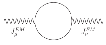
Figure 1: Leading order diagram for the calculation of the DC electrical conductivity in ChPT without collision effects.

III The DC conductivity in ChPT to leading order

III.1 The ideal gas contribution

Following the strict ChPT power counting, we should then start by considering the lowest order lagrangian ${\cal O}(p^{2})$ (the non-linear sigma model) coupled to an external photon. The lagrangian is given in gale84 . In the imaginary-time formalism we just take the same interaction vertices and electromagnetic current with the usual replacements for the Feynman rules, i.e, replacing all zeroth momentum components by discrete frequencies $k^{0}\rightarrow i\omega_{n}=2\pi inT$ and the loop integrals by Matsubara sums, i.e., $\int\!\frac{dk^{0}}{2\pi}\rightarrow iT\sum_{n=-\infty}^{\infty}$.

The dominant diagram to the current-current spectral function is that in Figure 1, which gives the following imaginary-time contribution to the spatial current-current correlation function :

$$\left[\Delta_{\beta}\right]^{0}_{jk}(i\nu_{m},|\vec{q}|)=e^{2}T\sum_{n=-\infty}^{\infty}\int\frac{d^{3}\vec{p}}{(2\pi)^{3}}\frac{(2p+q)_{j}(2p+q)_{k}}{\left[\omega_{n}^{2}+|\vec{p}|^{2}+m_{\pi}^{2}\right]\left[(\omega_{n}+\nu_{m})^{2}+|\vec{p}+\vec{q}|^{2}+m_{\pi}^{2}\right]}$$ (5)

with $m_{\pi}\simeq$ 140 MeV the pion mass. For small external momenta, we can drop the $q$ dependence in the numerator, so that we are led to the loop integral (37) with $k=1$, analyzed in the Appendix. With the results showed there, one has to this order:

$$\frac{\rho_{k}^{k}(\omega,|\vec{q}|)}{\omega}(\omega\rightarrow 0^{+},|\vec{q}|\rightarrow 0^{+})=\\ -\frac{e^{2}}{\pi}\theta(|\vec{q}|^{2}-\omega^{2})\frac{F_{1}\left[\omega^{2}/|\vec{q}|^{2};T\right]}{|\vec{q}|}$$

with $F_{1}$ defined in (45). We observe that the small energy and momentum limits give an ill-defined answer, due to the product of the vanishing denominator and the step function (see our comments in the Appendix). In other words, there are regions arbitrarily close to the origin in the $(\omega,|\vec{q}|)$ plane where we get different limits for the spectral function: it vanishes for the timelike region $|\vec{q}|^{2}<\omega^{2}$ and grows with $1/|\vec{q}|$ in the spacelike one $|\vec{q}|^{2}>\omega^{2}$. Therefore, in this case instead of specifying a particular order in taking the limits, we consider the Fourier transform of the contribution (III.1) back to position space, according to (3). We take electric fields slowly varying both in time and space, so that only the small $\omega$ and $|\vec{q}|$ limit of the spectral function is relevant. When doing so, we get a divergent contribution for the conductivity $\sigma=-\frac{e^{2}F_{1}(0;T)}{3\pi^{2}}\int_{0}^{\infty}dr$ to leading order in the derivative expansion of the electric field, where the dependence with the spatial length of the system is explicitly shown. This is physically expected since, as commented in the introduction, we are considering pions with zero width or infinite mean free path. In fact, this is nothing but the ideal gas result (no collisions) since by considering only the diagram in Figure 1 we are not taking into account the effect of pion interactions. Actually, to this order one would get the same answer, say, in scalar QED. Therefore in an ideal gas, the charged free pions travel throughout all the gas without interacting giving an infinite conductivity. Thus, for an external field constant over an infinite region, we should consider the effect of pion interactions so that the DC conductivity is actually proportional to the (finite) pion mean free path. This will require a more careful evaluation of ChPT diagrams, as we will show below.

III.2 Beyond the ideal gas: finite pion width.

Our previous discussion makes it clear that in order to get finite and physically sensible results for the DC conductivity, one has to consider the effect of a finite pion width. In the medium, the pion dispersion relation is $p^{2}=m_{\pi}^{2}+g(p_{0},|\vec{p}|;T)$ with $g$ a complex function. The pion width is $\Gamma_{p}(|\vec{p}|)=-\mbox{Im}\,g(E_{p},|\vec{p}|)/(2E_{p})<<E_{p}$ in ChPT with $E_{p}=\sqrt{|\vec{p}|^{2}+m_{\pi}^{2}}$ and we will neglect the ChPT corrections to $\mbox{Re}\,g$, since they are not relevant for our purposes. The lowest order contribution to $\mbox{Im}\,g$ in ChPT is ${\cal O}(p^{6})$ and can be calculated either by Kinetic Theory arguments gole89 or by evaluating the relevant diagrams schenk93 like the two-loop contribution shown in Figure 2a. The detailed results for $\Gamma_{p}$ can be found in those references. For most of our purposes here it will be enough to consider the dilute gas regime where $n_{B}(E_{p})\approx\exp(-E_{p}/T)<<1$:

$$\Gamma_{p}^{DG}=\frac{1}{2}\int\frac{d^{3}\vec{k}}{(2\pi)^{3}}\sigma^{\pi\pi}_{tot}(s)\frac{\sqrt{s(s-4m_{\pi}^{2})}}{2E_{k}E_{p}}\exp(-E_{k}/T)$$ (6)

where the Mandelstam variable $s=(E_{k}+E_{p})^{2}-|\vec{k}+\vec{p}|^{2}\geq 4m_{\pi}^{2}$ and $\sigma^{\pi\pi}_{tot}$ is the total elastic pion-pion cross section, that can be expressed as:

$$\sigma^{\pi\pi}_{tot}(s)=\frac{32\pi}{3s}\sum_{J=0}^{\infty}\sum_{I=0}^{2}(2J+1)(2I+1)|t_{IJ}|^{2}$$ (7)

in terms of partial waves of definite isospin $I$ and angular momentum $J$, for which we follow the same conventions for pion scattering as e.g. in gale84 . To lowest order in ChPT, i.e, $|t|^{2}={\cal O}(p^{4})$:

$$\sigma^{\pi\pi}_{tot}(s)=\frac{5s}{48\pi f_{\pi}^{4}}\left[1-\frac{16m_{\pi}^{2}}{5s}+\frac{37m_{\pi}^{4}}{10s^{2}}\right]$$ (8)

where $f_{\pi}\simeq 93$ MeV is the pion decay constant. Since the integrand in (6) is weighted by the Bose-Einstein factor, we expect that taking the leading order for $\sigma^{\pi\pi}_{tot}$ is enough for relatively low temperatures. We will comment below on the effect of considering higher order terms, for instance those respecting unitarity.

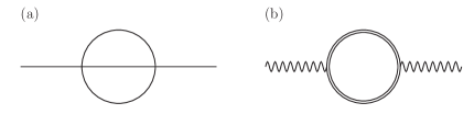
Figure 2: (a) A two-loop diagram contributing to the pion width. (b) Leading order current correlator with dressed pion lines.

The result (6) shows clearly how the pion traveling along the (dilute) medium with momentum $\vec{p}$ acquires a finite width by collisions with the medium constituents, the factor $\sqrt{s(s-4m_{\pi}^{2})}/(2E_{k}E_{p})$ being proportional to the relative velocity between the particles with momentum $p$ and $k$, expressed in relativistic form gole89 .

We consider then a pion propagator whose spectral function (see Appendix) is:

$$\rho_{\pi}(\omega,|\vec{p}|)=2\mbox{Im}\,iG^{R}(\omega,|\vec{p}|)=\frac{\Gamma_{p}}{E_{p}}\left[\frac{1}{(\omega-E_{p})^{2}+\Gamma_{p}^{2}}-\frac{1}{(\omega+E_{p})^{2}+\Gamma_{p}^{2}}\right]$$ (9)

Thus, the complex propagator is:

$$G(z,|\vec{p}|)=\frac{1}{E_{p}^{2}-\left[z+i\Gamma_{p}\mbox{sgn}(\mbox{Im}\,z)\right]^{2}}$$ (10)

for $\mbox{Im}\,z\neq 0$, which has a cut on the real axis and is analytic everywhere else in the complex $z$ plane.

We will denote by a double line, the pion propagator “dressed” with a nonzero width $\Gamma_{p}$, so that the leading order contribution to the current-current correlator is now given by diagram (b) in Figure 2. Its imaginary-time contribution is now

$$\left[\Delta_{\beta}\right]_{j}^{j}(i\nu_{m},|\vec{q}|=0)=\\ 4e^{2}T\sum_{n=-\infty}^{\infty}\int\frac{d^{3}\vec{p}}{(2\pi)^{3}}|\vec{p}|^{2}G_{\beta}(i\omega_{n},|\vec{p}|)G_{\beta}(i\omega_{n}+i\nu_{m},|\vec{p}|)$$

where $G_{\beta}[i\omega_{n}]=G[i\omega_{n}]$ in (10) for $n\neq 0$ and $G_{\beta}(n=0)=1/(\Gamma_{p}^{2}+E_{p}^{2})$ and where the $|\vec{q}|\rightarrow 0^{+}$ limit is now free of the ambiguities of the ideal gas case. We will evaluate the Matsubara sum in (III.2) following the same procedure as in valle02 . In this case, the result can be expressed in terms of integrals along the two cuts of $G$ at $\mbox{Im}\,z=0$ and $\mbox{Im}\,z=-\nu_{m}$ of the corresponding discontinuities of the $G$ function. The result is an analytic function for $i\nu_{m}$ off the real axis, so that we find for the retarded correlator ($\Delta^{R}(\omega)=-i\Delta_{\beta}(i\nu_{m}\rightarrow\omega+i\epsilon$)):

$$\left[\Delta^{R}\right]_{j}^{j}(\omega,|\vec{q}|=0) = 4e^{2}\int\frac{d^{3}\vec{p}}{(2\pi)^{3}}|\vec{p}|^{2}\left\{G_{\beta}(0)\left[G^{R}(\omega)-G^{A}(-\omega)\right]\right.$$ (11)

$$+ \int_{-\infty}^{\infty}\frac{dy}{2\pi}n_{B}(y)\left.\left[G^{R}(y)+G^{A}(y)\right]\left[G^{R}(y+\omega)-G^{A}(y-\omega)\right]\right\}$$

where we have omitted the $|\vec{p}|$ dependence in the propagators. Now, it is not difficult to see that the leading order term in the previous expression in the limits $\omega\rightarrow 0^{+}$ and $\Gamma<<E_{p}$ is an ${\cal O}(1/\Gamma)$ contribution coming from the products $G^{R}G^{A}$ which in this limit behave like a $\delta$ function:

$$\int_{-\infty}^{\infty}dyG^{R}(y)G^{A}(y)F(y)\simeq\frac{\pi}{4E_{p}^{2}\Gamma_{p}}\left[F(E_{p})+F(-E_{p})\right]$$ (12)

for $\Gamma_{p}<<E_{p}$.

This type of “pinching poles” contribution is crucial for the analysis of the conductivity. On the one hand, it is expected from Kinetic Theory considerations, as discussed in the introduction. On the other hand, it will lead to consider the effect of higher order diagrams, as we will do in the following sections. Up to this point, our result are analogous to those in jeon95 ; valle02 before specifying the explicit form of $\Gamma_{p}$ and discussing the power counting. Similar “pinching poles” contributions are obtained in real-time formalism calculations wahe99 ; amy01 .

Thus, we get for the DC conductivity to leading order:

Figure 3: Leading order for the DC conductivity. The left panel shows the dilute gas approximation (solid line) compared to the exact numerical result obtained by equation (13) with the full width calculated in gole89 ; schenk93 and to the $T<<m_{\pi}$ limit (dashed line) given by (16). In the right panel, the behaviour near $T\sim m_{\pi}$ is showed, where the dashed line is given by equation (17).

$$\sigma^{(0)}=\frac{e^{2}}{3T}\int\frac{d^{3}\vec{p}}{(2\pi)^{3}}\frac{|\vec{p}|^{2}}{E_{p}^{2}\Gamma_{p}}n_{B}(E_{p})\left[1+n_{B}(E_{p})\right]$$ (13)

where we have used that $n_{B}^{\prime}(x)=-n_{B}(x)\left[1+n_{B}(x)\right]/T$ and $n_{B}(-x)\left[1+n_{B}(-x)\right]=n_{B}(x)\left[1+n_{B}(x)\right]$. In Figure 3 we have plotted the leading order conductivity taking for $\Gamma_{p}$ the exact expression given in gole89 ; schenk93 including all factors of $n_{B}$, comparing it with the different approximations considered below.

The result (13) is very important for our purposes. It gives a finite and well-defined answer for the conductivity, with the correct dependence on the pion width and the density as expected from Kinetic Theory arguments. However, as commented before, the nonperturbative nature of the DC conductivity, reflected in the $1/\Gamma$ dependence, will make it necessary to examine higher order diagrams.

Let us evaluate the previous result for the conductivity in the dilute gas regime, which is valid for the range of temperatures of interest here. Thus, we replace the results (6) and (8) in (13), where we neglect the $n_{B}^{2}$ term. The result is showed in Figure 3 (solid line) where it is clear that the dilute gas regime in this case is an excellent approximation for temperatures below the pion mass. The conductivity of the pion gas grows for decreasing $T$, approaching the ideal gas limit discussed in section III.1. Note that both the pion density and the pion width vanish exponentially for $T\rightarrow 0^{+}$, so that it was not clear what should be the remaining $T$-dependence of their ratio. As we will show later, for very low temperatures $T<<m_{\pi}$, $\sigma\sim m_{\pi}\sqrt{m_{\pi}/T}$. This behaviour is nothing but the nonrelativistic limit predicted by Kinetic Theory arguments and indicates that there could be nonperturbative contributions of higher order diagrams in the very low $T$ region, where the typical $1/\Gamma$ insertions become larger.

For this reason, in the next section we will concentrate on the $T<<m_{\pi}$ limit. As we shall see, in this limit the analysis becomes simpler and our power counting arguments will be more clearly illustrated.

III.3 Very low temperatures

In the $T<<m_{\pi}$ limit, the relevant integrals in the previous expressions are dominated by the very low momentum region, weighted by $n_{B}(E_{k})\approx\exp(-m_{\pi}/T)\exp(-k^{2}/2m_{\pi}T)$. Thus, if we change $p\rightarrow\sqrt{m_{\pi}T}p$ in (13) and $k\rightarrow\sqrt{m_{\pi}T}k$ in (6), every power of a three-momentum integration variable $\vec{p}/m_{\pi}$ in those integrals counts as $\sqrt{m_{\pi}T}/m_{\pi}=\sqrt{T/m_{\pi}}$ and is therefore suppressed. Taking into account that in this limit $\sqrt{s(s-4m_{\pi}^{2})}\approx 2m_{\pi}|\vec{p}-\vec{k}|$ in (6), the angular integration in the expression for the thermal width can be performed and the low-$T$ result can be expressed in terms of error functions:

$$\Gamma_{p}^{LT}=\frac{m_{\pi}^{4}T^{2}}{E_{p}f_{\pi}^{4}}\exp(-m_{\pi}/T)f(\hat{p})$$ (14)

with

$$f(\hat{p})=\frac{23}{512\pi^{3}}\left[\exp(-\hat{p}^{2}/2)+\sqrt{\frac{\pi}{2}}\frac{1+\hat{p}^{2}}{\hat{p}}\mbox{Erf}(\hat{p}/\sqrt{2})\right]$$ (15)

and $\hat{p}=p/\sqrt{m_{\pi}T}$. What is important from this expression is that for $E_{p}\approx m_{\pi}$, $\Gamma_{p}\sim m_{\pi}^{3}T^{2}/f_{\pi}^{4}\exp(-m_{\pi}/T)$ times a dimensionless function of $\hat{p}$ only so that we get readily the dependence with $T,m_{\pi},f_{\pi}$ of the thermal width for very low temperatures, as the product $\Gamma\sim nv\sigma^{\pi\pi}_{tot}$ with $n\sim(\sqrt{m_{\pi}T})^{3}$ (mean density) and $v\sim\sqrt{m_{\pi}T}/m_{\pi}$ (mean velocity) in the nonrelativistic limit of very small pion momentum compared to its mass. We recall that the same nonrelativistic behaviour is recovered at very low temperatures for the shear viscosity, which grows with $\sqrt{T}$ dosa02 ; dolla04 .

Replacing the above result for the width in the $T<<m_{\pi}$ limit of (13) yields:

$$\sigma^{(0)}_{LT}=e^{2}m_{\pi}\frac{f_{\pi}^{4}}{6\pi^{2}m_{\pi}^{4}}\sqrt{\frac{m_{\pi}}{T}}\int_{0}^{\infty}d\hat{p}\frac{\hat{p}^{4}}{f(\hat{p})}\exp(-\hat{p}^{2}/2)\simeq 2.7e^{2}m_{\pi}\sqrt{\frac{m_{\pi}}{T}}$$ (16)

Therefore, for low $T$ we get a $\sqrt{m_{\pi}/T}$ behaviour for the conductivity in units of $m_{\pi}$. This result will be crucial for our chiral power counting analysis of higher terms in the DC conductivity and gives the behaviour near the origin plotted in Figure 3 where we compare (16) with the dilute gas approximation.

III.4 Higher temperatures

For temperatures up to the pion mass we can trust the dilute gas approximation, as shown in Figure 3. On the other hand, we do not expect ChPT to work much beyond that range. A fit to the numerical results for temperatures around $m_{\pi}$ assuming a single power form $aT^{b}$ gives:

$$\sigma^{(0)}(T)\simeq 0.82\ e^{2}m_{\pi}\left(\frac{f_{\pi}}{m_{\pi}}\right)^{4}\left(\frac{m_{\pi}}{T}\right)^{2.11}\qquad(T\raise 1.29167pt\hbox{$<$\kern-7.5pt\lower 4.30554pt\hbox{$\sim$}}m_{\pi})$$ (17)

The above behaviour with $T$ can be understood as follows. Consider the high temperature limit $T>>m_{\pi}$ in our previous expressions, which amounts to ignore the pion mass. Thus, for an integrand of the form $f(p)n_{B}(p)$, this is a better approximation for functions $f$ dominated by their high energy behaviour. In fact, in some cases the high-$T$ curve is approached for not very high temperatures, even when the dilute gas approximation still remains valid and it is not a bad approximation to neglect the pion mass in the dilute gas expressions, in order to get, at least qualitatively the behaviour for $T\raise 1.29167pt\hbox{$<$\kern-7.5pt\lower 4.30554pt\hbox{$\sim$}}m_{\pi}$. Consider for instance the total density of charged pions $N_{ch}=(1/\pi^{2})\int dkk^{2}n_{B}(E_{k})$. In the $T>>m_{\pi}$ limit we replace $n_{B}(E_{k})\simeq 1/(\exp(k/T)-1)$ and obtain $N_{ch}\simeq 2\zeta(3)T^{3}/\pi^{2}=2.4T^{3}/\pi^{2}$ whereas taking both the dilute gas and high-$T$ approximations, i.e. $n_{B}(E_{k})\simeq\exp(-k/T)$, gives $N_{ch}\simeq 2T^{3}/\pi^{2}$, which around $T\sim m_{\pi}$ is only about a 10$\%$ away from the exact curve. Something similar happens with the pion width $\Gamma_{p}$, for which the high-$T$ limit in the dilute gas expression (6) with the lowest order cross section in (8) gives $\Gamma_{p}\simeq 5T^{4}p/(12\pi^{3}f_{\pi}^{4})$. Note that it is crucial for this argument that the cross section grows with energy which in fact is not the physical case, since unitarity bounds the partial waves. Therefore, we see that implementing correctly the unitarity behaviour may change the behaviour of the thermal width and hence of the conductivity for intermediate and higher temperatures. We will examine this aspect in section V. Ignoring those possible corrections, the mean thermal width $\bar{\Gamma}=\int\Gamma_{p}n_{B}(E_{p})/\int n_{B}(E_{p})\simeq 5T^{5}/(4\pi^{3}f_{\pi}^{4})$ in this limit, in agreement with the analysis in gole89 . Therefore, we expect qualitatively for the conductivity $\sigma\sim e^{2}N_{ch}/(m_{\pi}\bar{\Gamma})\sim e^{2}m_{\pi}(f_{\pi}/m_{\pi})^{4}(m_{\pi}/T)^{2}$ as our above result (17) roughly confirms. Performing the same approximations, i.e., dilute gas in the chiral limit, directly in the expression (13) gives $\sigma^{(0)}=2\pi e^{2}f_{\pi}^{4}/(5T^{3})$ which is worse than the fit (17) at $T\raise 1.29167pt\hbox{$<$\kern-7.5pt\lower 4.30554pt\hbox{$\sim$}}m_{\pi}$, mostly because the integrand in (13) grows much slower with $p$ than in the case of the width.

We also note here that at higher temperatures, i.e, closer to the chiral phase transition, one has to be careful with the approach we are following throughout this work, since the thermal width becomes comparable to the mass, as a consequence of the loss of validity of ChPT. In fact, using our previous high-$T$ expression for the width gives $\bar{\Gamma}\simeq m_{\pi}/25$ at $T=$ 100 MeV but $\bar{\Gamma}\simeq 1.2m_{\pi}$ at $T=$200 MeV.

IV Higher order diagrams

Our previous analysis shows that the leading contributions to the DC electrical conductivity come from nonperturbative $1/\Gamma$ insertions for every pair of pion lines carrying equal momentum as the external four-momentum vanishes (double lines). Therefore, it is not obvious that diagrams of higher order in the chiral power counting are still suppressed with respect to the leading order analyzed in the previous section.

We recall that according to Weinberg’s power counting, the chiral power of a given diagram with two external photon lines is $e^{2}p^{D}$ with $D=2N_{L}+\sum_{d=2}(d-2)N_{d}$, $N_{L}$ being the number of loops and $N_{d}$ the number of vertices coming from the lagrangian of order $p^{d}$ in derivatives and meson masses. However, the presence of “pinching poles” modifies this picture. Let us assign a “nonperturbative” factor $Y$ to the contribution of every two internal double lines to the conductivity, so that we define $\sigma^{(0)}=e^{2}m_{\pi}Y$ and we call $X={\cal O}(p^{2})$ a chiral power, typically $X\simeq[m_{\pi}/(4\pi f_{\pi})]^{2}$. Thus, the diagram in Figure 2b analyzed in the previous section is ${\cal O}(Y)$ instead of the ${\cal O}(X)$ assigned by Weinberg’s power counting.

The next task is then to identify those diagrams which are dominant with this new power counting. In the case of a scalar $\lambda\phi^{4}$ theory, one has jeon95 $Y=1/\lambda^{2}$ and the dominant contributions are ladder diagrams of the type showed in Figure 4, which are all ${\cal O}(1/\lambda^{2})$ and have to be resummed, giving the results expected from Kinetic Theory. Other diagrams which naively could give larger contributions, like the “bubble” diagrams showed in Figure 5 have been shown to be subdominant. The same conclusion about the dominance of ladder diagrams holds in gauge theories amy00 ; valle02 ; amy01 .

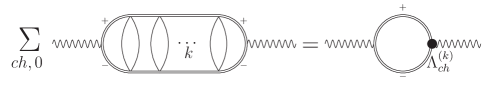
Figure 4: Ladder diagrams contributing to the electrical conductivity.

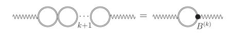
Figure 5: A generic bubble diagram with $k+1$ bubbles ($k\geq 1$).

The arguments based on the topology of the diagrams in the scalar theory apply directly to our case, so that we are led to examine the same class of diagrams. However, it must be pointed out that in ChPT there are important differences: first, we are actually dealing with a double counting in $X$ and $Y$ as explained before, which is a consequence of the importance of chiral loops in the power counting. Second, we are allowed to have derivative vertices and multiple vertices coming from lagrangians of different orders. And finally, there are two types of particles, charged and neutral, running in the internal lines and loops. This motivates our detailed analysis below, which main conclusions will be that here the ladder diagrams also dominate over other diagrams like the bubble ones, but their influence is not as important as it could be and can be safely considered subdominant with respect to the leading order result, within the ChPT validity range.

Let us start by considering then the ladder diagrams showed in Figure 4 where all the vertices come from the $d=2$ lagrangian. Note that only the internal lines running along the ladder can carry equal momentum when the external momentum vanishes, so that we keep the double line notation for those lines and the single line for the rung loops. Our power counting gives then ${\cal O}(X^{n}Y^{n+1})$ for the diagram with $n$ rungs. Therefore, those diagrams could in principle be of the same or even higher order than the zeroth order diagram analyzed in the previous section, depending of the relative size between $X$ and $Y$. Now recall that according to our previous analysis, the nonperturbative $Y$ factors are bigger the smaller the temperature, where typically $Y\sim\sqrt{m_{\pi}/T}$. It is therefore at very low $T$ where we have to be more concerned about these contributions. The detailed analysis in this regime is done in the next section, where we will see that at low $T$ one has to account also for the Bose-Einstein distributions emerging from the loops, which will give rise to additional suppressions.

IV.1 Ladder diagrams at very low $T$

For the analysis of the generic ladder diagram showed in Figure 4 we will follow similar steps as in valle02 . The contribution of the diagram with $k$ rungs to the current-current correlator is now:

$$\left[\Delta^{(k)}_{\beta}\right]_{j}^{j}(i\nu_{m},\vec{0})=e^{2}T\sum_{n=-\infty}^{\infty}\int\frac{d^{3}\vec{p}_{1}}{(2\pi)^{3}}2\vec{p}_{1}\cdot\vec{\Lambda}_{ch}^{(k)}(i\omega_{n}+i\nu_{m},i\omega_{n},\vec{p}_{1})$$

$$\times G_{\beta}(i\omega_{n},|\vec{p}_{1}|)G_{\beta}(i\omega_{n}+i\nu_{m},|\vec{p}_{1}|)$$ (18)

where $\vec{\Lambda}_{ch}^{(k)}$ is the effective $\pi^{+}\pi^{-}\gamma$ vertex made of $k$ rungs, as depicted in Figure 4, where the sum is made over all possible ways of inserting internal lines and vertices corresponding to charged and neutral pions, respecting charge conservation and including the corresponding combinatoric factors. Note that the two pairs of lines attached to the external lines are always charged, denoted in the figure by $+,-$ symbols. The lowest order effective vertex is $\vec{\Lambda}_{ch}^{(0)}=2\vec{p}_{1}$.

The effective vertices satisfy a recurrence relation which ultimately leads to integral equations corresponding to linearized Boltzmann equations jeon95 ; valle02 . The same equations for the effective vertices are obtained in the real-time formalism wahe99 ; amy01 . In our present case, the integral equations become a little more involved due to the presence of neutral and charged particles, as well as derivative vertices. However, for $T<<m_{\pi}$ an important simplification takes place: The leading order of the sum in Figure 4 for a given number of rungs $k$ is proportional to a single diagram where all vertices are replaced by constant vertices $m_{\pi}^{2}/f_{\pi}^{2}$ and therefore the spectral function of the rung integral is given by that of the loop correlator $J_{0}$ in (46), analyzed in the Appendix.

Let us justify our previous statement. We have seen in the previous section that the presence of a pair of double lines forces its momentum to be on shell at $p_{0}=\pm E_{p}$. Thus, consider the one-loop subgraph made of two “incoming” double lines and two “outgoing” ones. The two vertices contain different combinations of powers of two momenta or two masses in each vertex, where the momenta can be “external” (double lined) $p_{1},p_{2}$ or “internal” $k$ and $k+p_{1}\pm p_{2}$ (see details below). In addition, as we will see below, the integrals over $p_{1}$ and $p_{2}$ contain Bose-Einstein factors that, according to our very low $T$ counting, suppress powers of $\vec{p}_{1,2}/m_{\pi}$. Therefore, the leading contribution for $T<<m_{\pi}$ in $m_{\pi}^{4}$ or $p_{1,2}^{4}$ vertices is proportional to $m_{\pi}^{4}J_{0}(k)$, since $E_{1,2}\simeq m_{\pi}$. As for the powers involving “internal” momenta, using that $E_{1}+E_{2}\simeq 2m_{\pi}>>|\vec{p_{1}}-\vec{p_{2}}|>>E_{1}-E_{2}={\cal O}(|\vec{p}|_{1,2}^{2}/m_{\pi})$ and the relationship among the different one-loop thermal integral with momentum powers in the numerator discussed in Appendix A of glp02 , we have checked explicitly that we are left, to leading order, only with $m_{\pi}^{4}J_{0}$, $m_{\pi}^{3}J_{1}$ or $m_{\pi}^{2}J_{2}$ contributions to the imaginary part (spectral function) of the loops, which, as our analysis below will show, provides the relevant contributions to the ladder diagrams. The imaginary part of the $J_{\alpha}$ integrals is given in the Appendix. For $T<<m_{\pi}$ we can replace the Bose-Einstein distributions by Boltzmann exponentials and the relevant integrals can be explicitly evaluated, with the result that both for the thermal and for the unitarity cuts, the leading order of $\mbox{Im}\,J^{R}_{\alpha}$ are proportional to $m_{\pi}^{\alpha}\mbox{Im}\,J^{R}_{0}$ for $\alpha=1,2$.

Therefore, for $T<<m_{\pi}$ we have

$$\vec{\Lambda}_{ch}^{(k)}=\left(\frac{m_{\pi}}{f_{\pi}}\right)^{4k}\alpha^{(k)}\vec{\Lambda}^{(k)}$$ (19)

with $\alpha^{(k)}$ a purely numerical factor and

$$\vec{\Lambda}^{(k)}(i\omega_{m}+i\nu_{m},i\omega_{m},\vec{p}_{1}) = \int_{-\infty}^{\infty}\frac{d\omega^{\prime}}{2\pi}\int\frac{d^{3}\vec{p}_{2}}{(2\pi)^{3}}\rho(\omega^{\prime},|\vec{p}_{2}-\vec{p}_{1}|)T\sum_{n=-\infty}^{\infty}\vec{\Lambda}^{(k-1)}(i\omega_{n}+i\nu_{m},i\omega_{n},\vec{p}_{2})$$ (20)

$$\times \frac{G_{\beta}(i\omega_{n},|\vec{p}_{2}|)G_{\beta}(i\omega_{n}+i\nu_{m},|\vec{p}_{2}|)}{\omega^{\prime}-i(\omega_{n}-\omega_{m})}$$

where $\rho(\omega,|\vec{q}|)=2\mbox{Im}\,J_{0}^{R}(\omega,|\vec{q}|)=2\mbox{Im}\,I^{R}(\omega,|\vec{q}|;0)$ according to our notation in the Appendix. The above recurrence relation is depicted in Figure 6 and allows us to proceed along similar steps as in valle02 . By induction, we have that the only singularities of $\vec{\Lambda}^{(k)}(z+i\nu_{m},z,\vec{p})$ are the same two cuts as the propagator product in (20), i.e, at $\mbox{Im}\,z=0$ and at $\mbox{Im}\,z=-\nu_{m}$. This allows to perform the frequency sum in (18) in a similar manner as we did in the previous section and also the sum in the equation for the effective vertex (20), where in the latter case we have to consider, in addition to the cuts contribution, the pole contribution at $z=\omega^{\prime}+i\omega_{m}$. As in valle02 , the previous arguments on the analytic structure of the effective vertex imply that the analytic continuation $i\nu_{m}\rightarrow\omega+i\epsilon$ is well defined. Altogether, we find for the low-$T$ conductivity to leading order in $1/\Gamma$, using (12):

$$\sigma^{(k)}=\frac{e^{2}\alpha^{(k)}}{3T}\left(\frac{m_{\pi}}{f_{\pi}}\right)^{4k}\int\frac{d^{3}\vec{p}_{1}}{(2\pi)^{3}}\frac{|\vec{p}_{1}|^{2}}{E_{1}^{2}\Gamma_{1}}n_{B}(E_{1})\left[1+n_{B}(E_{1})\right]A^{(k)}(|\vec{p}_{1}|)$$ (21)

with

$$A^{(k)}(|\vec{p}_{1}|) = \frac{1}{|\vec{p}_{1}|^{2}}\int\frac{d^{3}\vec{p}_{2}}{(2\pi)^{3}}\frac{\vec{p}_{1}\cdot\vec{p}_{2}}{8E_{2}^{2}\Gamma_{2}}A^{(k-1)}(|\vec{p}_{2}|)\left\{\left[n_{B}(E_{2}-E_{1})-n_{B}(E_{2})\right]\rho\left(E_{2}-E_{1},|\vec{p}_{2}-\vec{p}_{1}|\right)\right.$$ (22)

$$- \left.\left[n_{B}(E_{2}+E_{1})-n_{B}(E_{2})\right]\rho\left(E_{2}+E_{1},|\vec{p}_{2}+\vec{p}_{1}|\right)\right\}$$

where we have also used that $\rho(\omega^{\prime})=-\rho(-\omega^{\prime})$ and we have denoted for the effective vertex $\vec{\Lambda}^{(k)}(x+i\epsilon,x-i\epsilon,\vec{p})=2\vec{p}\tilde{A}^{(k)}(|\vec{p}|;x)$ and $A^{(k)}(|\vec{p}|)=(\tilde{A}^{(k)}(|\vec{p}|;E_{p})+\tilde{A}^{(k)}(|\vec{p}|;-E_{p}))/2$ so that $A^{(0)}=1$. For simplicity, we have denoted $E_{1,2}=E_{p_{1},p_{2}}$ and so on for $\Gamma_{1,2}$ and omitted their explicit dependence with $|\vec{p}_{1}|,|\vec{p}_{2}|$.

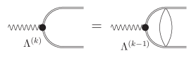
Figure 6: Recurrence relation between ladder vertices.

Let us comment on the result (22). The two terms in the right hand side correspond to evaluate the imaginary part of the rung loop at $p_{1}\pm p_{2}$ for on-shell $p_{1,2}$ “external” momenta. That is, those contributions arise from the $s,t$ channels of the $\pi\pi$ elastic scattering amplitude of the double lines in Figure 6, to one loop. Here we call by convenience ${\cal S}\equiv(E_{1}+E_{2},|\vec{p}_{1}+\vec{p}_{2}|)$ and ${\cal T}\equiv(E_{1}-E_{2},|\vec{p}_{1}-\vec{p}_{2}|)$. This interpretation will be very useful in our analysis of the different ChPT diagrams. In fact, note that the remaining $u$-channel contribution would be given by the contribution to the effective vertex of the bubble diagrams in Figure 5, since the loop integral of the bubble does not depend on $p_{1}$ and $p_{2}$, only on the external photon momentum $q$, i.e, we can identify ${\cal U}\equiv(\omega,\vec{0})$. Now we remark (see Appendix) that the imaginary part $\rho(E,|\vec{Q}|)$ is nonzero both for $E^{2}\geq|\vec{Q}|^{2}+4m_{\pi}^{2}$ (“unitarity” cut) and for $E^{2}\leq|\vec{Q}|^{2}$ (“thermal” cut). Since $s={\cal S}^{2}\geq 2m_{\pi}^{2}$, the $s$-channel is given by the unitarity contribution in (40) with $E=E_{1}+E_{2},\vec{Q}=\vec{p}_{1}+\vec{p}_{2}$, while $t={\cal T}^{2}\leq 2m_{\pi}^{2}$ and thus the $t$-channel is given by the thermal part in (43) with $E=E_{1}-E_{2},\vec{Q}=\vec{p}_{1}-\vec{p}_{2}$. Note that a consequence of this analysis is that, as announced, the bubble diagrams in Figure 5 are indeed suppressed in the $\omega\rightarrow 0^{+}$ limit since $u={\cal U}^{2}=\omega^{2}$ does not fall within any of the two cuts. This will be confirmed in section IV.3.

At very low $T$, there are further simplifications of the above equations, namely $n^{2}(E_{1,2}),n(E_{1}+E_{2})<<n(E_{1,2})\simeq\exp(-E_{1,2})/T$. Consistently, in the ${\cal S}$-channel, we can neglect the $T$-dependent part in the unitarity contribution (40). In the ${\cal T}$ channel, we can approximate in (43) the logarithm in the right hand side by $e^{-y_{0}/T}\left(1-e^{-|E_{1}-E_{2}|}\right)=e^{-(y_{0}+|E_{1}-E_{2}|)/T}/n_{B}(|E_{1}-E_{2}|)$. Since $y_{0}\geq m_{\pi}$, the leading contribution in that term comes from the $n_{B}(E_{2}-E_{1})$ term in (22), giving a net ${\cal O}(e^{-2m_{\pi}/T})$ contribution, the same as in the ${\cal S}$-channel and in the $\Gamma_{1}\Gamma_{2}$ in the denominator. The latter approximations are valid in the dilute gas regime, which as commented previously, extends to $T\raise 1.29167pt\hbox{$<$\kern-7.5pt\lower 4.30554pt\hbox{$\sim$}}m_{\pi}$. In addition, for $T<<m_{\pi}$ in the ${\cal S}$-channel, the product of the Bose-Einstein distributions $n(E_{1})n(E_{2})$ implies $E_{1,2}\simeq m_{\pi}+[|\vec{p}_{1,2}|^{2}/(2m_{\pi})]$ and hence $\sigma_{2p}\simeq|\vec{p}_{1}-\vec{p}_{2}|/(2m_{\pi})$. Finally, we have for $T<<m_{\pi}$:

$$\sigma^{(k)}_{LT}=e^{2}\alpha^{(k)}\frac{m_{\pi}}{3}\left(\frac{f_{\pi}}{m_{\pi}}\right)^{4}\sqrt{\frac{m_{\pi}}{T}}\int\frac{d^{3}\vec{y}_{1}}{(2\pi)^{3}}\frac{y_{1}^{2}}{f(y_{1})}A_{LT}^{(k)}\left(\sqrt{m_{\pi}T}y_{1}\right)\exp\left(-\frac{y_{1}^{2}}{2}\right)$$ (23)

$$A_{LT}^{(k)}\left(\sqrt{m_{\pi}T}y_{1}\right)=\frac{1}{32\pi y_{1}^{2}}\int\frac{d^{3}\vec{y}_{2}}{(2\pi)^{3}}\frac{\vec{y}_{1}\cdot\vec{y}_{2}}{|\vec{y}_{1}-\vec{y}_{2}|f(y_{2})}A_{LT}^{(k-1)}(\sqrt{m_{\pi}T}y_{2})\exp\left(-\frac{y_{2}^{2}}{2}\right)$$

$$\times\left\{\frac{|\vec{y}_{1}-\vec{y}_{2}|^{2}}{4}+\exp\left[\frac{1}{4}\left(y_{1}^{2}+y_{2}^{2}-\frac{1}{2}\frac{(y_{1}^{2}-y_{2}^{2})^{2}}{|\vec{y}_{1}-\vec{y}_{2}|^{2}}-\frac{1}{2}|\vec{y}_{1}-\vec{y}_{2}|^{2}\right)\right]\right\}$$

(24)

for $k\geq 1$, where the function $f$ is defined in (15) and we have rescaled $\vec{p}_{1,2}=\sqrt{m_{\pi}T}\vec{y}_{1,2}$ ($y_{1,2}\equiv|\vec{y}_{1,2}|$).

From the previous equations (23)-(24) we can draw one of our main conclusions: the low-$T$ effective vertex $A_{LT}^{(k)}\left(\sqrt{m_{\pi}T}y_{1}\right)$ is $T$-independent and hence, from (23) the correct order for the contribution of the $k$-rung ladder to the conductivity in our power counting scheme is $\sigma_{LT}^{(k)}=e^{2}m_{\pi}{\cal O}(X^{k}\sqrt{m_{\pi}/T})=e^{2}m_{\pi}{\cal O}(X^{k}Y)$ rather than the ${\cal O}(X^{k}Y^{k+1})$ following from direct inspection, as discussed at the beginning of this section. The independence of the LT effective vertex on $T$ follows from (24) by induction, since $A^{0}=1$. Then, the only dependence with $T$ in $\sigma_{LT}^{(k)}$ is the $1/\sqrt{T}$, the same as the lowest order (16). We can also understand why the “direct” counting misses $k$ inverse powers of $Y$. The reason is that the contribution from the spectral functions introduce an extra $\sqrt{T/m_{\pi}}$ factor inside the integrand in (24). These factors come from $\rho_{\cal S}\sim|\vec{p}_{1}-\vec{p}_{2}|/m_{\pi}$ and $\rho_{\cal T}\sim T/|\vec{p}_{1}-\vec{p}_{2}|$ before rescaling the integration variables. This reflects the fact that the imaginary parts are small at low $T$ due to the presence of the Bose-Einstein factors and represents one of the main differences between our analysis and the standard one in a coupling constant perturbation theory. The remaining ${\cal O}(X^{k})$ contribution comes from having $k$ chiral loops. To check explicitly our conclusions, we have evaluated numerically the one-rung contribution $k=1$ in (23)-(24) setting $\alpha^{(1)}=1$. We obtain $\sigma_{LT}^{(1)}/\sigma_{LT}^{(0)}\simeq 0.06$. The reason why this gives a slightly higher value than expected by power counting is the presence of a collinear effect in the ${\cal T}$-channel, coming from the region $\vec{y}_{1}\simeq\vec{y}_{2}$ in (24). The integral is convergent but that region enhances its value with respect to the ${\cal S}$ channel. In fact, for $k=1$ the ${\cal T}$-channel contribution is about five times larger than the ${\cal S}$-channel one, which has the expected chiral reduction mentioned above. Collinear effects of this kind are characteristic of these analysis and play a crucial role in gauge theories moore04 ; aurenche98 . In our case, this numerical enhancement does not spoil the perturbative nature of these contributions.

We can then conclude that the ladder diagrams at very low $T$, although representing the main contribution beyond leading order, are perturbative in the ChPT scheme. In numerical terms, the very low $T$ conductivity is given by (16) with a theoretical uncertainty of only about 5% in the multiplying coefficient.

IV.2 Ladder diagrams for $T\raise 1.29167pt\hbox{$<$\kern-7.5pt\lower 4.30554pt\hbox{$\sim$}}m_{\pi}$

Our previous analysis shows that the ladder diagrams are still chirally perturbative in the very low $T$ region, even though we should not miss the fact that their correct counting gives a much larger contribution than their standard ChPT one, namely $\sigma^{(k)}/\sigma^{(0)}={\cal O}(p^{2k})$ instead of the ${\cal O}(p^{4k})$ given by Weinberg’s theorem. The reason is the presence of the nonperturbative $Y$ factors, as we have seen. Following our chiral counting arguments for temperatures of the order of $m_{\pi}$, we realize first that now $Y\sim{\cal O}(1)$ around $T\sim m_{\pi}$. This means that we expect again $\sigma^{(k)}/\sigma^{(0)}={\cal O}(p^{2k})$ for the $k$-ladder diagram, coming from the rung loops. It must be reminded though that for these temperatures, the simplification of reducing any ladder diagram to one with constant vertices does not hold. In fact, for higher temperatures we expect derivative vertices to become increasingly important, but as long as $T$ remains within the ChPT applicability range (not much above the pion mass) we can consider all those diagrams perturbatively suppressed.

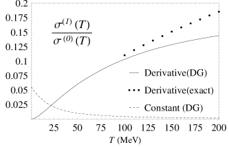
Figure 7: Estimation of the contribution of ladder diagrams for higher temperatures, with and without derivative vertices. The points correspond to the exact expressions without using the dilute gas approximation.

To check our previous comment we have evaluated numerically the ladder diagram with one rung and constant vertices, setting in (21)-(22) $k=1$ and $\alpha^{(1)}=1$ and performing only the dilute gas approximations mentioned in the previous section but not those specific of $T<<m_{\pi}$. We have also considered, for comparison, the contribution of a ladder diagram with one rung but with one possible combination of derivative vertices, namely, that obtained by taking $k=1$ in (21)-(22) but replacing the constant $(m_{\pi}/f_{\pi})^{4}$ factor by $|\vec{p}_{1}|^{4}/f_{\pi}^{4}$ in the integrand. The results are showed in Figure 7, where we have showed for comparison some points calculated without using the dilute gas approximation. Clearly, the derivative vertices become the more important ones at moderate and high temperatures, showing that the ladder diagrams have to be summed at temperatures close to the phase transition, where the ChPT power counting fails.

IV.3 Other diagrams

Following our previous arguments, it is not difficult to conclude that, as far as the ladder diagrams analyzed in sections IV.1 and IV.2 are perturbatively controlled in the chiral expansion, so are the same diagrams with vertices coming from the lagrangians ${\cal L}_{d}$ with $d>2$ and also ladder diagrams with rung loops made with more than four pion vertices.

As for the bubble diagram showed in Figure 5 which could in principle give nonperturbative contributions of ${\cal O}(Y^{n})$, our previous discussion based on the scattering of internal lines has already suggested that these diagrams do not receive contributions of ${\cal O}(1/\Gamma)$ to the conductivity. Let us show this in more detail. First, we define a $k$-bubble effective vertex $\vec{B}^{(k)}$ with $k\geq 1$ (see Figure 5) exactly as we have done in (18) for the ladder vertices $\vec{\Lambda}^{(k)}$. Given the structure of the bubble vertices, one readily realizes that, unlike the ladder ones, $\vec{B}^{(k)}(i\omega_{n}+i\nu_{m},i\omega_{n},\vec{p})$ is independent of the frequency and momentum of the external pion leg $(i\omega_{n},\vec{p})$ if only constant four-pion vertices are considered. Therefore, the contribution of those diagrams to the conductivity vanishes by parity, for instance by making $\vec{p}_{1}\rightarrow-\vec{p}_{1}$ in the integral analogous to (18). Thus, one needs derivative vertices to yield a nonvanishing contribution. In fact, following the parity argument, the only contributions of a $k+1$-bubble diagram which do not vanish by parity are those where all the four-pion vertices contain the factor $\vec{p}_{i}\cdot\vec{p}_{i+1}$ ($i=1,\dots,k$) where $p_{i}$ is the momentum running through the $i$-th bubble. We remark that we are considering only pion vertices coming from ${\cal L}_{2}$, higher order vertices being suppressed by Weinberg’s power counting and the same holds for bubbles made with more pion lines, say with vertices with more than four pions. Thus, the bubble effective vertices satisfy a recurrence relation of the form:

$$\vec{B}^{(k)}(i\nu_{m},\vec{p})=\int\frac{d^{3}\vec{p}_{2}}{(2\pi)^{3}}\frac{\vec{p}\cdot\vec{p}_{2}}{f_{\pi}^{2}}\ T\sum_{n=-\infty}^{\infty}\vec{B}^{(k-1)}(i\nu_{m},\vec{p}_{2})G_{\beta}(i\omega_{n},|\vec{p}_{2}|)G_{\beta}(i\omega_{n}+i\nu_{m},|\vec{p}_{2}|)$$ (25)

In fact, we should take into account that here can be also neutral pion loops in bubble diagrams with more than two bubbles, implying different vertex and combinatoric numerical factors in front of $\vec{p}_{i}\cdot\vec{p}_{i+1}$ for the $\pi^{0}\pi^{0}\pi^{+}\pi^{-}$, $\pi^{+}\pi^{-}\pi^{+}\pi^{-}$ and $(\pi^{0})^{4}$ vertices. Thus, we really have to define two effective vertices $\gamma\pi^{+}\pi^{-}$ and $\gamma\pi^{0}\pi^{0}$, the latter starting with one bubble and one has then two coupled recurrence relations between those vertices, instead of the single one in (25). However, that merely complicates the calculation but does not change our main conclusion, namely that bubble diagrams are subdominant. Hence, for simplicity, let us show it for the case in which all $4\pi$ vertices contribute simply as $\vec{p}_{i}\cdot\vec{p}_{i+1}/f_{\pi}^{2}$ and all internal lines are charged. Proceeding then as in section IV.1, we realize that the calculation is particularly simple now since the vertex (25) is still independent of the frequency of the external leg $i\omega_{m}$ and therefore there is no pole contribution, unlike (20). Then, the Matsubara sum is just the same as that in (III.2). We get, after analytic continuation $i\nu_{m}\rightarrow\omega+i\epsilon$ and to leading order in $1/\Gamma$ and $\omega\rightarrow 0^{+}$:

$$\vec{B}^{(k)}(\omega,\vec{p})=\frac{i\omega}{T}\int\frac{d^{3}\vec{p}_{2}}{(2\pi)^{3}}\frac{\vec{p}\cdot\vec{p_{2}}}{f_{\pi}^{2}}\frac{n(E_{2})\left[1+n(E_{2})\right]}{4E_{2}^{2}\Gamma_{2}}\vec{B}^{(k-1)}(\omega,\vec{p}_{2})\equiv\frac{i\omega\vec{p}}{f_{\pi}^{2}}F^{(k-1)}(\omega;T)$$ (26)

for $k\geq 1$, where the last line holds by Euclidean covariance and defines the scalar function $F$, which satisfies then the recurrence relation:

$$F^{(k)}(\omega;T)=\frac{i\omega I(T)}{f_{\pi}^{2}}F^{(k-1)}(\omega;T)=2I(T)\left[\frac{i\omega I(T)}{f_{\pi}^{2}}\right]^{k}$$ (27)

where $I(T)$ is the integral appearing in the lowest order conductivity in (13), namely $\sigma^{(0)}=4e^{2}I(T)$ and we have used that $B_{j}^{(0)}=\Lambda_{j}^{(0)}=2p_{j}$ so that $F^{(0)}=2I(T)$.

From the above results, we note that the two main differences between the bubble effective vertices and the ladder ones are, first, that for small $\omega$, the contribution of the $k+1$-bubble diagram to the conductivity is ${\cal O}(\omega^{k})$ and, second, that the bubble effective vertices are not all real, $B^{(k)}$ is real for $k$ even and purely imaginary for $k$ odd, to leading order in $1/\Gamma$. This confirms our discussion in section IV.1 about the role of the different diagrams as related to the “scattering” of the internal pion lines. The one-bubble diagram amounts to the tree level contribution to the scattering in ChPT which is always real. The first diagram giving a nonvanishing contribution to the scattering spectral function is the two-bubble one, but it vanishes as $\omega\rightarrow 0^{+}$ as corresponds to the ${\cal U}$ channel.

The simple form of the bubble vertices allows to perform explicitly their contribution to the conductivity, since they form basically a geometric series according to (27). The fact that bubble diagrams can be summed is a well-established result and holds also in other analysis of transport coefficients jeon95 . In fact, we remark that in our case it is consistent to sum them, following our power counting arguments, since the bubble diagrams are neither reduced by chiral loops like the ladder ones (all lines are double) nor by higher order pion vertices if all pion vertices come from ${\cal L}_{2}$.

Thus, the contribution of the sum of the bubble diagrams to the conductivity is of the form:

$$\sigma_{bub} = \frac{e^{2}}{3}\lim_{\omega\rightarrow 0^{+}}\frac{1}{T}\int\frac{d^{3}\vec{p}}{(2\pi)^{3}}\frac{n(E_{p})\left[1+n(E_{p})\right]}{4E_{p}^{2}\Gamma_{p}}\mbox{Re}\,\sum_{k=1}^{\infty}2\vec{p}\cdot\vec{B}^{(k)}(\omega,\vec{p})$$ (28)

$$= 2e^{2}\lim_{\omega\rightarrow 0^{+}}\mbox{Re}\,\sum_{k=1}^{\infty}F^{(k)}(\omega)=\sigma^{(0)}(T)\lim_{\omega\rightarrow 0^{+}}\mbox{Re}\,\frac{i\omega I(T)/f_{\pi}^{2}}{1-i\omega I(T)/f_{\pi}^{2}}$$

$$= {\cal O}(\omega^{2})\sigma^{(0)}(T)$$

and the same conclusion, i.e, $\sigma_{bub}={\cal O}(\omega^{2})\sigma^{(0)}(T)$ is reached when considering the full contributions of charged and neutral diagrams, as commented before. We wish to stress that the leading order in the bubble vertices comes from the “pinching poles” in products $G_{R}G_{A}$ and carries the ${\cal O}(\omega/\Gamma)$ contributions analyzed above. Taking the next to leading order could give a nonvanishing contribution as $\omega\rightarrow 0^{+}$ but with no $1/\Gamma$ terms (the $I(T)$ integrals above) and therefore suppressed by the ordinary chiral power counting of the loops so that, typically, the $\omega I(T)$ factors in the sum (28) would be replaced by an ${\cal O}(p^{2})$ contribution. Therefore, our conclusion is that the bubble diagrams are subdominant for all temperatures within the validity range of ChPT.

V Unitarity, high $T$ behaviour and photon production

One of the conclusions of the preceding sections is that the behaviour of the conductivity with temperature is greatly influenced by that of the thermal width, as expected from physical arguments. At the same time, the thermal width in the dilute gas regime (6) grows with $T$ according to the growing of the partial waves and cross-section with energies. We have been using the low-energy leading order in ChPT (8) which grows with energy $s$. However, we know that partial waves should be bounded in energy, as a consequence of unitarity. We recall that the unitarity condition for the $S$-matrix translates into

$$\mbox{Im}\,t_{IJ}(s)=\sigma_{2p}(s)|t_{IJ}|^{2}$$ (29)

for the elastic $\pi\pi$ scattering partial waves ($s\geq 4m_{\pi}^{2}$ and below any inelastic threshold) where $\sigma_{2p}(s)=\sqrt{1-4m_{\pi}^{2}/s}$ is the two-pion phase space. The unitarity condition (29) implies that the modulus and the phase $\delta_{IJ}$ (the phase shifts) of the partial waves are related as $|t_{IJ}|=\sin\delta_{IJ}/\sigma_{2p}$ which means in particular that $|t_{IJ}|$ is bounded as energy increases, as commented above.

The ChPT partial waves only satisfy unitarity perturbatively, for instance $\mbox{Im}\,t_{IJ}^{(4)}=\sigma_{2p}|t_{IJ}^{(2)}|^{2}$ where the chiral expansion is $t_{IJ}=t_{IJ}^{(2)}+t_{IJ}^{(4)}+\dots$. They are not bounded and they cannot reproduce a resonant behaviour, like those appearing in the $I=J=0$ (the $\sigma$ or $f_{0}(600)$) and $I=J=1$ channels (the $\rho(770)$). However, it is possible to construct amplitudes satisfying exact unitarity and matching the low-energy ChPT expansion. In doing so, we will follow the so called Inverse Amplitude Method (IAM) iam relying on its remarkable success to describe meson-meson scattering data up to 1 GeV and to generate the low lying resonances gp02 . We remark that through this unitarization procedures, physical resonances are generated dynamically with masses and widths in agreement with those listed in the Particle Data Book pdg . Furthermore, the unitarization procedure can be extended to finite temperature, providing a consistent description of the thermal properties of resonances, such as the widening of the $\rho$ in the thermal bath dglp02 . The IAM unitarized partial waves for $\pi\pi$ elastic scattering are simply given by $t^{IAM}=[t^{(2)}]^{2}/(t^{(2)}-t^{(4)})$. The same formula is valid at finite temperature, where the fourth order thermal amplitudes have been calculated in glp02 .

We are then interested in the effect of unitarity on our previous results. The first important comment is that unitarity is not expected to change our low $T$ results, where only the low-energy region of the $\pi\pi$ scattering contributes. We expect more significant corrections for $T$ near $m_{\pi}$. The effect of unitarity on the pion width has already been discussed in schenk93 . As it follows from our previous comments, the unitarized width $\Gamma_{p}$ has a softer behaviour with $p$, which, according to our arguments in section III.4 means a larger contribution to the conductivity as $T$ increases, as compared with the non-unitarized one.

We replace then the unitarized IAM partial waves in (7) in order to obtain the unitarized width (6) and conductivity (13). Several comments are in order here. First, we are considering only the contribution of the partial waves with lower angular momentum, i.e., $IJ=00,11,20$. Partial waves with $J>1$ are negligible for $\sqrt{s}\leq$ 1 GeV gp02 and so they are for the temperatures involved here. Second, we are not including the finite temperature corrections to the partial waves calculated in glp02 . The reason is that those are dilute gas corrections to the partial waves and therefore would contribute at ${\cal O}(n_{B}^{2})$ to the thermal width in (6), i.e, at the same order that other contributions that we have neglected. However, we should bear in mind that thermal corrections to the amplitudes describe correctly important features such as the changes in the mass and width of the thermal resonances, as it has been indeed observed in Relativistic Heavy Ion Collisions, so that their effect could be qualitatively important. Finally, we are using the same set of chiral parameters for the $d=4$ lagrangian as in dglp02 , ensuring that the mass and width of the $\rho$ agree with the $T=0$ values in pdg .

Figure 8: We show the result obtained in the dilute gas regime with the unitarized partial waves (solid line) compared to the perturbative ones up to ${\cal O}(p^{4})$ (dashed line).

The results of the unitarized conductivity are showed in Figure 8, where we compare with the non-unitarized one including ${\cal O}(p^{4})$ terms in the partial waves, i.e., $t=t^{(2)}+t^{(4)}$. The most relevant feature is that for temperatures about the pion mass, the curve for the conductivity changes notably its behaviour with respect to the perturbative one for $T\raise 1.29167pt\hbox{$>$\kern-7.5pt\lower 4.30554pt\hbox{$\sim$}}$ 100 MeV. As expected from our previous comments, the unitarized conductivity decreases much more slowly with temperature. In fact, extrapolating this result for high enough $T$, the conductivity starts increasing with $T$, although very slowly as it can be seen in Figure 8. Therefore, unitarity, and ultimately the presence of resonances in the medium, is responsible for the change of behaviour from the low $T$ to the high $T$ phases. In this sense, we notice that the main effect arising from unitarization comes from the $00$ channel which has the vacuum quantum numbers and is therefore more sensible to changes near the chiral phase transition. We also remark that this softening of the temperature behaviour when unitarization effects are taken into account holds also for the shear viscosity dolla04 .

Although clearly we should not trust our approximations much beyond $T\simeq$ 150 MeV, it is interesting to note that all the high-$T$ analysis in the QGP phase shows a typical linear increasing behaviour $\sigma\propto T$ amy00 , which follows simply from high-$T$ dimensional analysis. Therefore, when we include unitarity (which may not be the only relevant effect at these temperatures), the conductivity slowly tends to its expected high-$T$ behaviour. In fact, extrapolating our results to arbitrarily high temperature yields a linear behaviour for $T\sim$ 600 MeV.

The high-$T$ QCD analysis are not applicable to temperatures close to the transition, say $T\sim$ 200 MeV, where one should in principle appeal either to lattice results or to phenomenological models. The lattice calculation in gupta04 predicts $\sigma\simeq 0.35T$ for $T\simeq 1.5T_{c}$. However, one should be careful when interpreting results coming from the lattice in the $\omega\rightarrow 0^{+}$ limit of the current-current correlators resco . In fact, there are notable discrepancies between different lattice analysis. For instance, the conductivity extrapolated from the dilepton rate in karsch02 for $T\simeq 1.5T_{c},3T_{c}$ vanishes identically, as pointed out in blage05 . This is equivalent to state that the photon spectrum vanishes at vanishing energy from the timelike region (see our comments in section V.1).

Our results show the behaviour from below the chiral phase transition, although with our present level of approximation we can only make qualitative statements at this point. On the one hand, we predict a nonzero conductivity, which, as we discuss in the next section, is compatible with having a sizable contribution to the photon emissivity from the hadronic phase. On the other hand, although unitarity makes the conductivity grow with $T$ as we approach the chiral phase transition (note that the nonunitarized result vanishes asymptotically) the values we obtain are still much smaller than those in gupta04 . For instance, we have $\sigma/T\simeq 0.007$ around $T=$ 200 MeV. Apart from possible ambiguities in the lattice analysis, we should bear in mind that several effects that we have not accounted for in our perturbative treatment, like resummation of ladder diagrams or the contribution of heavier particles, become important at those temperatures.

V.1 Photon production

Another possibility to extract physical information related to the electrical conductivity is to consider the photon emissivity coming from the hadronic phase. The photon differential rate emerging from an equilibrated system is directly related with the EM current-current correlator as alam01 :

$$\omega\frac{dR_{\gamma}}{d^{3}\vec{q}}=\frac{1}{8\pi^{3}}n_{B}(\omega)\rho^{\mu}_{\mu}(\omega=|\vec{q}|)$$ (30)

The Ward Identity $q^{\mu}\rho_{\mu\nu}=0$ implies $\rho^{0}_{0}(\omega\neq 0,\vec{q}=0)=0$ so that the electrical conductivity provides direct information about the vanishing energy limit ($\omega\rightarrow 0^{+}$) in the static region gupta04 ; blage05 simply as $\omega dR_{\gamma}/d^{3}\vec{q}(\omega\rightarrow 0^{+},\vec{q}=0)=3T\sigma(T)/(4\pi^{3})$, i.e, a nonzero conductivity implies a constant value for the photon yield near the origin.

With this motivation in mind, we will compare our results for the conductivity for temperatures physically relevant in a Relativistic Heavy Ion environment with some recent theoretical and experimental analysis of the low-energy hadronic photon spectrum. Among the theoretical works, one can find the virial expansion approach followed in steele96 with nonstrange mesons only, extended in steele97 to include baryon density. More recent analysis follow the conventional Kinetic Theory approach, where all possible photon-producing reactions of the type $1+2\rightarrow 3+\gamma$ are evaluated, 1,2,3 being meson degrees of freedom $\pi,\rho,K,...$ parametrized in an effective lagrangian with explicit resonances included alam01 ; rawa99 ; turaga04 . The present experimental data are described remarkably well for $\omega>$200 MeV when all the relevant processes are evaluated and finite density effects are accounted for turaga04 . However, it is worth mentioning that recent analysis of the WA98 experiment wa98 at CERN have produced data at lower transverse momentum, showing a slight systematic enhancement with respect to theoretical predictions. At those low energies, the hadronic gas contribution seems to dominate over the QGP one.

The low-energy rate with nonstrange mesons in steele96 , which deals then with the same degrees of freedom as our approach, reaches a maximum value of about 3 $\times 10^{-5}$ GeV^-2fm^-5 (for $T=$150 MeV) at $\omega\sim$ 400 MeV and then drops to zero at the origin. When including baryons in the same approach steele97 the behaviour is the same but the maximum is at $\omega\sim$ 200 MeV and grows up to about 4 $\times 10^{-4}$ GeV^-2fm^-4. The results in rawa99 for the hadronic gas are similar to those in steele96 ; steele97 except that the curve with baryon density decreases monotonically for $\omega\geq$ 200 MeV. In turaga04 , more relevant channels have been included, the most interesting result being that there are also meson contributions that do not vanish when approaching the origin, for instance those involving $\pi\rho a_{1}$ mesons. The latter contributions amount to almost twice more photons near the origin that in the earlier work rawa99 . We remark that the prediction in turaga04 is the one used in the experimental WA98 paper wa98 to compare with data and it remains below the lowest energy points. Using the unitarized width, we get for the vanishing energy photon rate $3T\sigma/(4\pi^{3})\simeq 3.7\times 10^{-3}$ GeV^-2fm^-4 at $T=$150 MeV. Therefore, we predict a sizable value of the hadronic photon rate at the origin. A linear extrapolation of the low energy curve ($\omega\simeq$ 200 MeV) in turaga04 to the origin gives a value of about 2 $\times 10^{-3}$ GeV^-2fm^-4 at $T=$150 MeV. This is an indication that our prediction lies in the correct range.

We will now try to establish a more direct comparison with experimental data, bearing in mind that our approach only gives information about the value very close to the origin. One then has to integrate the photon rate in (30) over space-time and average over the photon rapidity turaga04 in order to obtain the experimentally measured photon yield $\omega dN_{\gamma}/d^{3}\vec{q}$ as a function of $q_{T}$, the component of the photon momentum transverse to the collision axis in the laboratory frame. Obviously, the results depend heavily on the hydrodynamical space-time evolution for the conditions applicable to a particular experiment. We will just give here rough estimates and for that purpose we will neglect transverse flow and assume a simple Bjorken’s hydrodynamical description lebellac ; petho02 so that $\omega=q_{T}\cosh(y-\eta)$ with $y$ and $\eta$ the photon and fluid rapidities respectively. Therefore, our value at $\omega\rightarrow 0^{+}$ translates directly into the value of the yield at $q_{T}\rightarrow 0^{+}$. As for the space-time integration, we use the typical value lebellac ; petho02 for the nuclear transverse radius $R_{A}\simeq$ 1.3 fm $A^{1/3}\simeq$ 7.7 fm for ²⁰⁸Pb and change to proper time $\tau$ and rapidity $\eta$ coordinates. In the Bjorken’s limit and for $q_{T}\rightarrow 0^{+}$, there is no dependence with rapidity so that we have simply to multiply by the expansion velocity petho02 $\Delta\eta_{nucl}=2\mbox{arccosh}(\sqrt{s}/(2AGeV)\simeq 10.1$ for the WA98 collision energy $\sqrt{s}=158$ A GeV. With these approximations, the photon yield at the origin is given by:

$$\omega\frac{dN_{\gamma}}{d^{3}\vec{q}}(q_{T}\rightarrow 0^{+})\simeq\pi R_{A}^{2}\Delta\eta_{nucl}\int_{\tau_{i}}^{\tau_{f}}\frac{3T(\tau)\sigma(T(\tau))}{4\pi^{3}}\tau d\tau$$ (31)

A crude estimate is obtained by assuming a purely thermal hadronic phase, i.e., a constant temperature. Taking proper time values $\tau_{i}=$ 1 fm/$c$ and $\tau_{f}=$ 13 fm/$c$ turaga04 and $T=150$ MeV, this gives $dN_{\gamma}/d^{3}\vec{q}(q_{T}=0)\simeq 5.8\times 10^{2}$. A more realistic approximation is to take the cooling law of an ideal gas $T(\tau)=T_{i}(\tau_{i}/\tau)^{1/3}$ lebellac which is probably still rather crude for mesons at moderate or high temperatures. Taking $\tau_{i}=$ 3 fm/$c$, more appropriate for the hadronic phase, $\tau_{f}=$ 13 fm/$c$ and $T_{i}=$ 170 MeV, we get $T_{f}=$ 104 MeV which is of the order of the freeze-out temperature. Inserting this law in (31) with the unitarized conductivity in Fig.8 we obtain $dN_{\gamma}/d^{3}\vec{q}(q_{T}=0)\simeq 5.6\times 10^{2}$ although this result is very sensitive to variations in temperature.

Taking the two points of smallest $p_{T}$ in wa98 and simply extrapolating them to the origin with a straight line gives $dN_{\gamma}/d^{3}\vec{q}(q_{T}=0)\simeq 5\times 10^{2}$. Therefore, our results are compatible with the recent data, in the sense of a naive linear extrapolation from the origin and not forgetting that we are bordering the applicability range of our approach, in addition to the many approximations performed to arrive to a number comparable with experiment. In any case, our analysis would suggest that purely thermal cuts in pion-pion annihilation (there is no $T=0$ real photon production from $\pi\pi$ annihilation for energies below $2m_{\pi}$) with a nonzero pion thermal width may be a relevant effect . In this sense, it should be borne in mind that the pion thermal width is not considered in steele96 ; steele97 ; alam01 ; rawa99 ; turaga04 since it does not play any role at the energies of interest for the photon yield considered in those works. On the other hand, our approach could be too limited to describe correctly the effect of some resonances like the $a_{1}$. It is even unclear whether our prediction at small energies has simply to be added to previous hadronic ones, since we are extracting the photon rate from the self-energy and not from individual processes. What is more clear in this respect is that the contribution analyzed here does not come from baryonic sources.

VI Conclusions

In this work we have analyzed the DC electrical conductivity of a pion gas at low temperatures within the framework of Chiral Perturbation Theory. The nonperturbative nature of transport coefficients is reflected in the need of including the thermal pion width in the calculations, in order to avoid “pinching poles” singularities. Physically, this allows to account for the relevant in-medium pion collisions and gives rise to the leading order contribution in the inverse width consistently with Kinetic Theory. The leading order in ChPT shows a decreasing behaviour with temperature, behaving like $\sigma\sim\sqrt{m_{\pi}/T}$ for $T<<m_{\pi}$ as expected from the nonrelativistic limit of Kinetic Theory. For higher temperatures, $\sigma\sim(m_{\pi}/T)^{2}$ for $T\raise 1.29167pt\hbox{$<$\kern-7.5pt\lower 4.30554pt\hbox{$\sim$}}m_{\pi}$ if unitarity corrections are not included in elastic pion scattering.

A very important part of our analysis has been the role of higher order diagrams which, although naively suppressed, are enhanced by powers of the inverse width. As it happens in other theories, the dominant diagrams are uncrossed ladder ones, which in our case can be interpreted in terms of pion scattering of the internal lines. A careful evaluation of the ladder diagrams shows that they can be still considered perturbative in ChPT at low temperatures. This is particularly important at very low temperatures $T<<m_{\pi}$ where the nonperturbative contributions are larger. In that regime we have been able to show exactly that ladder diagrams are perturbative, so that they merely renormalize the coefficient of the $1/\sqrt{T}$ behaviour of the conductivity by subleading corrections in ChPT. Although collinearly enhanced, our numerical analysis shows that these corrections are typically around 5%. As temperature increases, ladder diagrams become more important, the most relevant contributions coming from ladders with derivative vertices. At temperatures near the chiral phase transition it is not clear that ladder diagrams can be neglected, since ChPT is not applicable. In fact, at those high temperatures we expect other effects to become important, like the presence of kaon states.

Another important point concerns unitarity. We have showed that the conductivity changes qualitatively its behaviour with temperature for $T>$100 MeV as a consequence of implementing unitarity of the partial waves in the thermal width. This provides a more physical picture as far as the behaviour of partial waves with energy and the presence of resonances in the thermal bath are concerned. The unitarized conductivity increases slowly for increasing $T$, which seems to be consistent with lattice and analytical analysis far beyond the transition point. In fact, the most important contribution in this respect comes from the partial wave corresponding to the $f_{0}(600)$ with vacuum quantum numbers $I=J=0$. We have also considered some possible consequences of our results regarding the photon spectrum. The lack of precise experimental and lattice knowledge about the zero frequency limit, together with the own limitations of our approach do not allow to draw very quantitative conclusions. However, our analysis implies that there should be sizable effects for very low energy hadronic photon production and this result is consistent with recent theoretical low-energy analysis and compatible with naive extrapolations of experimental data. In our opinion, this makes the analysis presented here useful in order to understand some of the current discrepancies regarding the low-energy results. However, this is just but the first step and we will pursue a more detailed analysis in the near future, including some effects discarded here that could be important in more realistic situations, like the presence of kaon states, nonzero pion and baryon chemical potentials or thermal modifications of resonances.

Summarizing, despite its limitations as the temperature approaches the phase transition, we believe that our present work provides a useful and physically relevant example where the diagrammatic approach to transport coefficients can be implemented in a controlled way. More realistic applications to physical observables such as the photon spectrum are under way and will be reported elsewhere.

*

Appendix A Thermal correlators

A.1 General Properties

We review here some of the results needed throughout the text, mostly to fix our conventions and notation. For a given, rotationally invariant, correlator $\Delta(z,|\vec{q}|)$ analytical for any complex $z$ off the real axis, it is convenient to introduce its spectral function as:

$$\Delta(z,|\vec{q}|)=\int_{-\infty}^{\infty}\frac{d\omega^{\prime}}{2\pi}\frac{\rho(\omega^{\prime},|\vec{q}|)}{\omega^{\prime}-z}$$ (32)

The advanced and retarded correlators are then given by :

$$\Delta^{R,A}(\omega,|\vec{q}|)=\mp i\Delta(z=\omega\pm i\epsilon,|\vec{q}|)$$ (33)

where $\omega\in{\mathbb{R}}$. Note that, with our definitions $\rho=2\mbox{Re}\,\Delta^{R}=2\mbox{Im}\,(i\Delta^{R})$.

On the other hand, the imaginary-time correlator is given by the values on the discrete Matsubara frequencies:

$$\Delta_{\beta}(i\omega_{n},|\vec{q}|)=\Delta(z=i\omega_{n},|\vec{q}|)$$ (34)

When performing a perturbative calculation in the imaginary-time formalism, one can express the final result as an analytic function off the real axis, once all the sums over internal frequencies have been performed. Then, the imaginary-time result is continued analytically to external real frequencies simply from (33) and (34) as:

$$\Delta^{R,A}(\omega,|\vec{q}|)=\mp i\Delta_{\beta}(i\omega_{n}\rightarrow\omega\pm i\epsilon,|\vec{q}|)$$ (35)

The usual case is that when the correlator is a two-point function, like the field $\phi$ itself or a conserved current. In that case one has in position space:

$$G^{R,A}(t,\vec{x}) = \pm\theta(\pm t)<[\phi(t,\vec{x}),\phi(0)]>$$

$$G_{\beta}(\tau,\vec{x}) = <T_{C}\phi(-i\tau,\vec{x})\phi(0)>$$

$$\rho(t,\vec{x}) = <[\phi(t,\vec{x}),\phi(0)]>$$ (36)

where the brackets denote thermal expectation values, $t\in{\mathbb{R}}$ and $T_{C}$ denotes time ordering along the imaginary-time contour $C$ defined as the straight line $\tau\in[0,\beta]$. Note that, from the above equations, $\rho(\omega,|\vec{q}|)=-\rho(-\omega,|\vec{q}|)$, as expected for scalar spectral functions.

A.2 Loop integrals

In the analysis of the conductivity, we find loops involving the imaginary-time correlators:

$$I(i\omega_{m},|\vec{Q}|;k)=iT\sum_{n=-\infty}^{\infty}\int\frac{d^{3}\vec{p}}{(2\pi)^{3}}\frac{|\vec{p}|^{2k}}{\left[\omega_{n}^{2}+|\vec{p}|^{2}+m^{2}\right]\left[(\omega_{n}+\omega_{m})^{2}+|\vec{p}+\vec{Q}|^{2}+m^{2}\right]}$$ (37)

with $k=0,1$.

Performing the Matsubara sum in the usual way lebellac , one arrives to a function analytical in $i\omega_{m}$ off the real axis, so that we find for the retarded correlator:

$$\mbox{Im}\,I^{R}(\omega,|\vec{Q}|;k)=\pi\sum_{s_{1},s_{2}=\pm 1}\int\frac{d^{3}\vec{p}}{(2\pi)^{3}}|\vec{p}|^{2k}\frac{s_{1}s_{2}}{4E_{p}E_{p+Q}}\left[1+n\left(s_{1}E_{p}\right)+n\left(s_{2}E_{p+Q}\right)\right]$$

$$\times\delta\left[\omega-s_{1}E_{p}-s_{2}E_{p+Q}\right]$$ (38)

where $E_{q}^{2}=|\vec{q}|^{2}+m^{2}$ and $n_{B}(x)=\left(e^{\beta x}-1\right)^{-1}$ is the Bose-Einstein distribution function. The two $s_{1}=s_{2}$ contributions require $s\geq 4m^{2}$ ($s=\omega^{2}-|\vec{Q}|^{2}$) and give the unitarity cut appearing in the analysis of thermal scattering glp02 . Performing the angular integrations with the delta function, it can be written as:

$$\left[\mbox{Im}\,I^{R}(\omega,|\vec{Q}|;k)\right]_{unit}=\frac{\mbox{sgn}(\omega)\theta(s-4m^{2})}{16\pi|\vec{Q}|}\int_{y_{-}}^{y_{+}}dy\left(y^{2}-m^{2}\right)^{k}\left[1+n_{B}(y)+n_{B}(|\omega|-y)\right]$$ (39)

where $y_{\pm}=(|\omega|\pm|\vec{Q}|\sigma_{2p}(s))/2\geq m$ for $s\geq 4m^{2}$ and $\sigma_{2p}(s)=\sqrt{1-4m^{2}/s}$ is the phase space of two particles of equal mass $m$.

The case $k=0$ can be solved in terms of elementary functions:

$$\left[\mbox{Im}\,I^{R}(\omega,|\vec{Q}|;0)\right]_{unit}=\frac{\mbox{sgn}(\omega)\theta(s-4m^{2})}{16\pi}\left[\sigma_{2p}(s)+\frac{2T}{|\vec{Q}|}\log\left[\frac{1-\exp(-y_{+}/T)}{1-\exp(-y_{-}/T)}\right]\right]$$ (40)

On the other hand, in the limit $|\vec{Q}|\rightarrow 0^{+}$ (center of mass limit in the scattering case) we find:

$$\left[\mbox{Im}\,I^{R}(\omega,|\vec{Q}|\rightarrow 0^{+};k)\right]_{unit}=\frac{\mbox{sgn}(\omega)\theta(s-4m^{2})}{16\pi}\sigma_{T}(\omega)\left[\left(\frac{|\omega|}{2}\right)^{2}-m^{2}\right]^{k}$$ (41)

where $\sigma_{T}(\omega)=\sigma_{2p}(\omega^{2})\left[1+2n_{B}(|\omega|/2)\right]$ is the two-particle thermal phase space, which can be interpreted in terms of enhancement and absorption in the thermal bath glp02 .

Let us analyze now the two $s_{1}=-s_{2}$ contributions. First, it is not difficult to see that these two integrals are identical and contribute only for $s\leq 0$. Unlike the unitarity cut, this cut is purely thermal, i.e, is only present for $T\neq 0$. Integrating the delta function, their contribution to $\mbox{Im}\,I^{R}$ is:

$$\left[\mbox{Im}\,I^{R}(\omega,|\vec{Q}|;k)\right]_{ther} = -\frac{\mbox{sgn}(\omega)\theta(-s)}{16\pi|\vec{Q}|}\int_{y_{0}}^{\infty}dy\left[n_{B}(y+|\omega|)-n_{B}(y)\right]$$ (42)

$$\times \left[(y^{2}-m^{2})^{k}+((y+|\omega|)^{2}-m^{2})^{k}\right]$$

where $y_{0}=-y_{-}=(-|\omega|+|\vec{Q}|\sigma_{2p}(s))/2\geq m$ for $s\neq 0$. For $k=0$:

$$\left[\mbox{Im}\,I^{R}(\omega,|\vec{Q}|;0)\right]_{ther}=\frac{T}{8\pi|\vec{Q}|}\mbox{sgn}(\omega)\theta(-s)\log\left[\frac{1-e^{-(y_{0}+|\omega|)/T}}{1-e^{-y_{0}/T}}\right]$$ (43)

Now, taking the limit $|\vec{Q}|\rightarrow 0^{+}$ with $m$ and $T$ fixed implies necessarily $\omega\rightarrow 0^{+}$ since this is a space-like contribution. More precisely, $y_{0}\simeq\frac{m|\vec{Q}|}{\sqrt{-s}}$, so that:

$$\left[\mbox{Im}\,I^{R}(\omega\rightarrow 0^{+},|\vec{Q}|\rightarrow 0^{+};k)\right]_{ther}=-\frac{1}{8\pi}\theta(-s)\frac{\omega}{|\vec{Q}|}\left[F_{k}\left[\omega^{2}/|\vec{Q}|^{2};T\right]+{\cal O}\left(\frac{|\omega|}{m},\frac{|\omega|}{T}\right)\right]$$ (44)

where:

$$F_{k}(x;T)=\int_{\frac{m}{\sqrt{1-x}}}^{\infty}dy(y^{2}-m^{2})^{k}n_{B}^{\prime}(y)$$ (45)

for $0\leq x<1$. Note that $F_{k}(x)<0$, $\lim_{x\rightarrow 1^{-}}F_{k}(x)=0$ and that the small energy and momentum limits (44) do not coincide necessarily with taking directly $|\vec{Q}|=0$ with $\omega\neq 0$, which gives a vanishing contribution due to the step function.

Following similar steps as above, it is not difficult to obtain the imaginary part of loop integrals with more powers of $i\omega_{n}$ in the numerator:

$$J_{\alpha}(i\omega_{m},|\vec{Q}|)=iT\sum_{n=-\infty}^{\infty}\int\frac{d^{3}\vec{p}}{(2\pi)^{3}}\frac{(i\omega_{n})^{\alpha}}{\left[\omega_{n}^{2}+|\vec{p}|^{2}+m^{2}\right]\left[(\omega_{n}+\omega_{m})^{2}+|\vec{p}+\vec{Q}|^{2}+m^{2}\right]}$$ (46)

with $\alpha$ a positive integer or zero. We have analyzed the $\alpha=0$ case previously. For arbitrary $\alpha$ we get:

$$\left[\mbox{Im}\,J^{R}_{\alpha}(\omega,|\vec{Q}|)\right]_{unit}=\frac{\left[\mbox{sgn}(\omega)\right]^{\alpha+1}\theta(s-4m^{2})}{16\pi|\vec{Q}|}\int_{y_{-}}^{y_{+}}dy(-y)^{\alpha}\left[1+n_{B}(y)+n_{B}(|\omega|-y)\right]$$ (47)

$$\left[\mbox{Im}\,J^{R}_{\alpha}(\omega,|\vec{Q}|)\right]_{ther}=-\frac{\left[\mbox{sgn}(\omega)\right]^{\alpha+1}\theta(-s)}{16\pi|\vec{Q}|}\int_{y_{0}}^{\infty}dy\left[y^{\alpha}+(-1)^{\alpha}(y+|\omega|)^{\alpha}\right]$$

$$\times\left[n_{B}(y+|\omega|)-n_{B}(y)\right]$$ (48)

References

- (1) S. Weinberg, Physica A96, 327 (1979).
- (2) J. Gasser and H. Leutwyler, Annals Phys. 158, 142 (1984).
- (3) J. Gasser and H. Leutwyler, Phys. Lett. B184, 83 (1987); P.Gerber and H.Leutwyler, Nucl. Phys. B321, 387 (1989).
- (4) J.L.Goity and H.Leutwyler, Phys. Lett. B228, 517 (1989).
- (5) A. Schenk, Phys. Rev. D47, 5138 (1993).
- (6) A. Gómez Nicola, F. J. Llanes-Estrada and J. R. Peláez, Phys. Lett. B550, 55 (2002).
- (7) A.Dobado, A.Gómez Nicola, F.Llanes-Estrada and J.R.Peláez, Phys. Rev. C66, 055201 (2002).
- (8) S.Jeon, Phys. Rev. D52, 3591 (1995).
- (9) P.Arnold, G.D.Moore and L.G.Yaffe, JHEP 0011:001 (2000).
- (10) M.A.Valle Basagoiti, Phys. Rev. D66, 045005 (2002).
- (11) E.M.Lifshitz and L.P.Pitaevskii, Physical Kinetics (Pergamon Press 1981).
- (12) S.Gupta, Phys. Lett. B597, 57-62 (2004).
- (13) M.Prakash, M.Prakash, R.Venugopalan and G.M.Welke, Phys. Rev. Lett. 70, 1228 (1993).
- (14) D.Davesne, Phys. Rev. C53, 3069 (1996).
- (15) A.Dobado and S.N.Santalla, Phys. Rev. D65, 096011 (2002).
- (16) A.Dobado and F.J.LLanes-Estrada,Phys. Rev. D69, 116004 (2004).
- (17) J.Alam et al, Ann.Phys.286, 159-248 (2001) and references therein.
- (18) P.Aurenche, F.Gelis, R.Kobes and H.Zaraket, Phys. Rev. D58, 085003 (1998).
- (19) P.Arnold, G.D.Moore and L.G.Yaffe, JHEP 0111:057 (2001).
- (20) F.Gelis, H.Niemi, P.V.Ruuskanen and S.S.Räsänen, J.Phys.G.Nucl.Part.Phys. 30, S1031-S1035 (2004).
- (21) J. P. Blaizot and F. Gelis, Eur. Phys. J. C43, 375 (2005).
- (22) J.V.Steele, H.Yamagishi and I.Zahed, Phys. Lett. B384 255 (1996).
- (23) J.V.Steele, H.Yamagishi and I.Zahed, Phys. Rev. D56, 5605 (1997).
- (24) R.Rapp and J.Wambach, Eur. Phys. J. A6, 415 (1999).
- (25) S.Turbide, R.Rapp, C.Gale, Phys. Rev. C69, 014903 (2004).
- (26) M.Le Bellac, Thermal Field Theory (Cambridge University Press, 1996).
- (27) G.D.Mahan, Many-Particle Physics (Kluwer Academic , Plenum US, 2000).
- (28) T.S.Evans, Nucl. Phys. B374, 340 (1992); R.Baier and A.Niégawa, Phys. Rev. D49, 4107 (1994).
- (29) J.Schwinger, J.Math.Phys. 2, 407 (1961); L.V.Keldysh, Sov.Phys.JETP 20, 1018 (1965); Y.Takahashi and H.Umezawa, Collect.Phenom.2, 55 (1975); A.J.Niemi and G.W.Semenoff, Ann.Phys.(N.Y.) 152, 105 (1984); Nucl. Phys. B230, 181 (1984).
- (30) R.Kobes, Phys. Rev. D42, 562 (1990); Phys. Rev. D43, 1269 (1991).
- (31) E.Wang and U.Heinz, Phys. Lett. B471, 208 (1999).
- (32) G.D.Moore, J.Phys.G. 30 S775-S782 (2004).
- (33) T. N. Truong, Phys. Rev. Lett. 61, 2526 (1988); Phys. Rev. Lett. 67, 2260 (1991); A. Dobado, M.J.Herrero and T.N. Truong, Phys. Lett. B235, 134 (1990); A.Dobado and J.R. Peláez, Phys. Rev. D47, 4883 (1993); Phys. Rev. D56, 3057 (1997).
- (34) A.Gómez Nicola and J.R.Peláez, Phys. Rev. D65:054009 (2002).
- (35) S. Eidelman et al., Phys. Lett. B592, 1 (2004).
- (36) G. Aarts and J. M. Martinez Resco, JHEP 0204, 053 (2002).
- (37) F.Karsch, E.Laermann, P.Petreczky, S.Stickan and I.Wetzorke, Phys. Lett. B530 (2002) 147-152.
- (38) M. M. Aggarwal et al. [WA98 Collaboration], Phys. Rev. Lett. 93, 022301 (2004).
- (39) T.Peitzmann and M.Thoma, Phys.Rep.364, 175 (2002).