A Model of Dark Energy and Dark Matter

Abstract

A dynamical model for the dark energy is presented in which the “quintessence” field is the axion, $a_{Z}$, of a spontaneously broken global $U(1)_{A}^{(Z)}$ symmetry whose potential is induced by the instantons of a new gauge group $SU(2)_{Z}$. The $SU(2)_{Z}$ coupling becomes large at a scale $\Lambda_{Z}\sim 10^{-3}\,eV$ starting from an initial value $M$ at high energy which is of the order of the Standard Model (SM) couplings at the same scale $M$. A perspective on a possible unification of $SU(2)_{Z}$ with the SM will be briefly discussed. We present a scenario in which $a_{Z}$ is trapped in a false vacuum characterized by an energy density $\sim(10^{-3}\,eV)^{4}$. The lifetime of this false vacuum is estimated to be extremely large. Other estimates relevant to the “coincidence issue” include the ages of the universe when the $a_{Z}$ potential became effective, when the acceleration “began” and when the energy density of the false vacuum became comparable to that of (baryonic and non-baryonic) matter. Other cosmological consequences include a possible candidate for the weakly interacting (WIMP) Cold Dark Matter as well as a scenario for leptogenesis. A brief discussion on possible laboratory detections of some of the particles contained in the model will also be presented.

I Introduction

The nature of the dark energy (responsible for an accelerating universe acceleration ) is one of the deepest problem in contemporary cosmology. Supernovae observations at redshifts $1.25\leq z\leq 1.7$ when combined with cosmic microwave background (CMB) and cluster data gave an equation of state $w=p/\rho=-1.02+0.13-0.19$ riess and are consistent with a generic $\Lambda\,CDM$ model where $w=-1$ independently of $z$. Most recently, distance measurements of 71 high redshift Type Ia supernovae by the Supernova Legacy Survey (SNLS) up to $z=1$ combined with measurements of baryon acoustic oscillations by the Sloan Digital Sky Survey also fits a flat $\Lambda\,CDM$ with constant $w=-1.023\pm 0.090\pm 0.054$ snls . Future proposed measurements to test whether or not $w$ is time-varying will be of crucial importance. Various forms of Quintessence had been proposed to describe the present accelerating universe sahni . A generic feature of these models is the presence of a time-varying $w$. However, it is a known fact that the dark energy is subdominant at higher values of redshift which makes it much harder to detect the $z$-dependence of $w$ doran . Until this is resolved, it is practically impossible to distinguish the class of quintessence models with time-varying $w$ from one in which $w$ is practically constant and is equal to $-1$. However, one should keep in mind that several quintessence models typically predict $w>-1$ now with many of them having $w\gtrsim-0.8$. In fact, one can try to reconstruct the quintessence potential as had been done recently by sahlen whose analysis of recent data appeared to favor a cosmological constant.

Is there a quintessence scenario in which $w=-1$ for a large range of $z$ and which mimics the $\Lambda\,CDM$ model? Can such a scenario make predictions that go beyond the accelerating universe issue and that can be tested experimentally? These are the types of questions we wish to address in this paper.

There exists a well-known phenomenon that can be readily applied to the search for models that mimic $\Lambda\,CDM$: The idea of the false vacuum. It has been used in the construction of models of early inflation (although a “standard model” is yet to be found) kolb . In its simplest version, the potential of a scalar field (whose nature depends on a given model) develops two local minima: a “false” and a “true” one, as the temperature drops below a certain critical value. In this class of models, the universe is trapped in the false vacuum and the total energy density of the universe is soon dominated by the energy of this false vacuum, leading to an exponential expansion. For the early inflation case, models have been constructed to deal with the so-called graceful exit problem, i.e. how to go from the false vacuum to the true vacuum without creating gross inhomogeneities, resulting in a class of so-called new inflationary scenarios (see kolb for an extensive list of references).

Is the fact that present measurements appear to be consistent with a flat $\Lambda\,CDM$ model with a constant $w=-1$ an indication that we have been and are still living in a false vacuum with an energy density $\rho_{vac}\sim(10^{-3}\,eV)^{4}$? If that is the case, when did we get trapped in that false vacuum and when are we getting out of it? And where does this false vacuum come from?

In this paper, we would like to explore the above possibility and present a model for the false vacuum scenario. First, we will postulate the existence of an unbroken gauge group $SU(2)_{Z}$ su2 and show that, starting with a gauge coupling comparable in value to the Standard Model (SM) couplings at some high energy scale ($\sim 10^{16}\,GeV$), it becomes strongly interacting at a scale $\sim 10^{-3}\,eV$. This new gauge group $SU(2)_{Z}$ zophos can be seen to come from the breaking $E_{6}$ bj into $SU(2)_{Z}\otimes SU(6)$, where $SU(6)$ can, as one possible scenario, first break down to $SU(3)_{c}\otimes SU(3)_{L}\otimes U(1)$ and then to $SU(3)_{c}\otimes SU(2)_{L}\otimes U(1)_{Y}$, the details of which will be dealt with in a separate paper hung2 . Next, we will list the particle content of our model and present an argument showing how the $SU(2)_{Z}$ instanton-induced axion potential can provide a model for the aforementioned false vacuum with the desired energy density jain . We will compute the transition rate to the true vacuum and show that it is plausible that the universe was trapped in this false vacuum and will be accelerating for a very, very long time. We then show that the particle spectrum of the model contains fermions which have the necessary characteristics of being candidates for a WIMP Cold Dark Matter. Finally, we will briefly discuss the possibility of SM leptogenesis in our model where the SM lepton number violation comes from the asymmetry in the decay of a “messenger” scalar field which carries both $SU(2)_{Z}$ and $SU(2)_{L}$ quantum numbers. A more detailed version of this leptogenesis scenario will appear in a separate paper hung3 . We will end with a brief discussion of the possibility of detection for the messenger field and the $SU(2)_{Z}$ fermions (CDM candidates).

II $SU(2)_{Z}$ as a new strong intersection at extremely low energy

In this section, we would like to discuss the possibility of a new asymtotically-free gauge group, $SU(2)_{Z}$, which can grow strong at an extremely low energy scale such as $\sim 10^{-3}\,eV$, starting with a coupling of the same order as the Standard Model couplings at high energies and, in particular, at some “GUT” scale $\sim 10^{16}\,GeV$ su2 . We first show how, using the particle content of the model, the $SU(2)_{Z}$ gauge coupling evolves from an initial value which is close to those of the SM couplings at a typical GUT scale $M$ to $\alpha_{Z}=g_{Z}^{2}/4\,\pi\sim 1$ at a scale $\Lambda_{Z}\sim 10^{-3}\,eV$. (In a GUT scenario like the $E_{6}$ example mentioned above, $\Lambda_{Z}$ could be seen as being generated from the GUT scale $M$.) Turning things around, one can ask the following question: If one would like to have $\alpha_{Z}=g_{Z}^{2}/4\,\pi\sim 1$ at a scale $\sim 10^{-3}\,eV$, what should the initial value of $\alpha_{Z}$ be at high energies in order for this condition to be fulfilled? As we shall see below, it turns out that this initial value is correlated with the $SU(2)_{Z}$ particle content and on the masses of the SM-singlet $SU(2)_{Z}$ fermions in an interesting way: $\alpha_{Z}(M)$ decreases as the masses of the $SU(2)_{Z}$ fermions increase. If we wish $\alpha_{Z}(M)$ to be close in value to the SM couplings, we find the masses of these fermions to be in the $GeV$ region, an interesting range for the dark matter as we shall see below. We will then discuss a possible origin of $SU(2)_{Z}$ from a grand unified point of view with more details to be presented elsewhere hung2 .

II.1 The $SU(2)_{Z}$ model and its particle content

The gauge group that we are concerned with is

$$G_{SM}\otimes SU(2)_{Z}\,,$$ (1)

where

$$G_{SM}=SU(3)\otimes SU(3)_{L}\otimes U(1)_{Y}\,.$$ (2)

The $SU(2)_{Z}$ particle content is as follows.

• Two fermions: $\psi^{(Z)}_{(L,R),i}=(1,1,0,3)$ under $SU(3)\otimes SU(2)_{L}\otimes U(1)_{Y}\otimes SU(2)_{Z}$, where $i=1,2$. The reasons for having two such fermions will be made clear below when we discuss the evolution of the $SU(2)_{Z}$ gauge coupling.

• Messenger scalar fields: $\varphi^{(Z)}=(\varphi^{(Z),0},\varphi^{(Z),-})=(1,2,Y_{\varphi}=-1,\,2)$ or two ${\tilde{\bm{\varphi}}}_{i}^{(Z)}=({\tilde{\bm{\varphi}}}^{(Z),0},{\tilde{\bm{\varphi}}}^{(Z),-}_{i})=(1,2,Y_{\tilde{\varphi}}=-1,\,3)$ under $SU(3)\otimes SU(2)_{L}\otimes U(1)_{Y}\otimes SU(2)_{Z}$, where $i=1,2$. Again the reason for having two ${\tilde{\bm{\varphi}}}$ (one of which will be assumed to be much heavier than the other) will be made clear below. Briefly spaeking, it has to do with the SM leptogenesis mechanism proposed at the end of the manuscript. For this reason, the scenario with two ${\tilde{\bm{\varphi}}}$ is more attractive than that in which one has only a $SU(2)_{Z}$ doublet $\varphi^{(Z)}$. We discuss both cases in the section on the gauge coupling evolution for completeness and for the purpose of comparison.

• Complex singlet scalar field: $\phi_{Z}=(1,1,0,1)$.

Finally, the SM particles are assumed to be singlets under $SU(2)_{Z}$, namely

• $q_{L}=(3,2,1/3,1)$; $u_{R}=(3,1,2/3,1)$; $d_{R}=(3,1,-1/3,1)$.

• $l_{L}=(1,2,-1,1)$; $e_{R}=(1,1,-2,1)$.

The above notations are meant to be generic for each SM family. We do not list the right-handed neutrinos, which we believe to exist, since they are singlets under $G_{SM}\otimes SU(2)_{Z}$ and are not relevant for the present analysis.

A few words are in order concerning the above choices. The fermions are chosen to be triplets of $SU(2)_{Z}$ in order to “slow down’ the evolution of the $SU(2)_{Z}$ coupling. The messenger scalar fields are chosen for two purposes: 1) to contribute to the $\beta$ function of $SU(2)_{Z}$ and 2) to connect the aforementioned fermions to their SM counterparts. The singlet complex scalar field is introduced in the manner of Peccei-Quinn PQ . The instanton-induced “axion-potential” is used to model the dark energy, as we shall see below.

II.2 The Lagrangian of the model

The Lagrangian for $G_{SM}\otimes SU(2)_{Z}$ is

$${\cal L} = {\cal L}_{SM}+{\cal L}^{Z}_{kin}+{\cal L}_{yuk}+{\cal L}_{CP}-V(|\tilde{\bm{\varphi}}^{(Z)}|^{2}\;{\rm or}\;|\varphi^{(Z)}|^{2})$$ (3)

$$-V(|\phi_{Z}|^{2})\,,$$

where ${\cal L}_{SM}$ is the well-known SM Lagangian, which does not need to be explicitely written down here, and where

$${\cal L}^{Z}_{kin} = -\frac{1}{4}{\bf G}_{\mu\nu}^{(Z)}.{\bf G}^{(Z),\mu\nu}+(\sum_{i}\frac{1}{2}(D_{\mu}\,\tilde{\bm{\varphi}}_{i}^{(Z)})^{{\dagger}}.(D^{\mu}\,\tilde{\bm{\varphi}}_{i}^{(Z)})\,$$ (4)

$${\rm or}\;\frac{1}{2}(D_{\mu}\,\varphi^{(Z)})^{{\dagger}}(D^{\mu}\,\varphi^{(Z)}))$$

$$+\sum_{i}i\bar{\psi}^{(Z)}_{(L,R),i}\not\!D\psi^{(Z)}_{(L,R),i}\,,$$

$${\cal L}_{yuk} = \sum_{i}\,\sum_{m}(g_{\tilde{\varphi}_{1}\,m}^{i}\,\bar{l}_{L}^{m}\,\tilde{\bm{\varphi}}_{1}^{(Z)}\,\psi^{(Z)}_{i,R}+g_{\tilde{\varphi}_{2}\,m}^{i}\,\bar{l}_{L}^{m}\,\tilde{\bm{\varphi}}_{2}^{(Z)}\,\psi^{(Z)}_{i,R})$$ (5)

$$+\sum_{i}K_{i}\,\bar{\psi}^{(Z)}_{L,i}\,\psi^{(Z)}_{R,i}\,\phi_{Z}+h.c.\,,$$

$${\cal L}_{CP}=\frac{\theta_{Z}}{32\,\pi^{2}}{\bf G}_{\mu\nu}^{(Z)}.\tilde{{\bf G}}^{(Z),\mu\nu}\,.$$ (6)

The covariant derivative acting on $\varphi$ is given by

$$D_{\mu}\varphi^{(Z)}=(\partial_{\mu}-ig\frac{\bm{\tau}}{2}.{\bf W}_{\mu}+i\frac{g^{{}^{\prime}}}{2}B_{\mu}-ig_{Z}\frac{\bm{\tau}}{2}.{\bf A}^{(Z)}_{\mu})\varphi^{(Z)}\,,$$ (7a)

$$D_{\mu}\tilde{\bm{\varphi}}_{i}^{(Z)}=((\partial_{\mu}-ig\frac{\bm{\tau}}{2}.{\bf W}_{\mu}+i\frac{g^{{}^{\prime}}}{2}B_{\mu}-ig_{Z}{\bf T}.{\bf A}^{(Z)}_{\mu})\tilde{\bm{\varphi}}_{i}^{(Z)}\,,$$ (7b)

and that acting on $\psi^{(Z)}_{(L,R),i}$ is given by

$$D_{\mu}\psi^{(Z)}_{(L,R),i}=(\partial_{\mu}-ig_{Z}{\bf T}.{\bf A}^{(Z)}_{\mu})\psi^{(Z)}_{(L,R),i}\,,$$ (8)

where $(T^{i})_{jk}=i\,\epsilon^{ijk}$. In Eqs. (4,6, 7, 8), we use boldfaces to express explicitely the triplet nature of the $SU(2)_{Z}$ gauge fields and $\tilde{\varphi}$. Also, in Eq. (4,5), the sum over $m$ means that we are summing over the number of SM families while the sum over $i$ means that we are summing over the two $SU(2)_{Z}$ fermions and the two triplet scalars. The coefficients $g_{\tilde{\varphi}_{1}\,m}$, $g_{\tilde{\varphi}_{2}\,m}$, and $K_{i}$ are, in general, complex.

II.3 Global symmetries

The Lagrangian written above exhibits a $U(1)_{A}^{(Z)}$ global symmetry. In fact, Eqs.(5,6) are invariant under the following $U(1)_{A}^{(Z)}$ phase transformation:

$$\psi^{(Z)}_{i}\rightarrow e^{i\alpha\gamma_{5}}\,\psi^{(Z)}_{i}\,,$$ (9a)

$$\psi^{(Z)}_{L,i}\rightarrow e^{-i\alpha}\,\psi^{(Z)}_{L,i}\,,$$ (9b)

$$\psi^{(Z)}_{R,i}\rightarrow e^{i\alpha}\,\psi^{(Z)}_{R,i}\,,$$ (9c)

$$\phi_{Z}\rightarrow e^{-2i\alpha}\,\phi_{Z}\,,$$ (9d)

$$\theta_{Z}\rightarrow\theta_{Z}-4\,\alpha\,,$$ (9e)

$$l_{L}^{m}\rightarrow e^{i\alpha}\,l_{L}^{m}\,,$$ (9f)

$$\tilde{\bm{\varphi}}_{i}^{(Z)}\rightarrow\tilde{\bm{\varphi}}_{i}^{(Z)}\,.$$ (9g)

Since ${\cal L}_{SM}$ contains Yukawa couplings between the SM leptons to the SM Higgs fiels $\phi_{SM}$ of the form $\bar{l}_{L}^{m}\,\phi_{SM}\,l_{R}^{n}$ (and also $\bar{l}_{L}^{m}\,\tilde{\phi}_{SM}\,\nu_{R}^{n}$ for the neutral leptons), where $l_{R}^{n}$ ($\nu_{R}^{n}$) denotes the charged (neutral) right-handed leptons, it will be invariant under the above $U(1)_{A}^{(Z)}$ global symmetry provided

$$l_{R}^{m}\;(\nu_{R}^{m})\rightarrow e^{i\alpha}\,l_{R}^{m}\;(\nu_{R}^{m})\,,$$ (10)

when we use the transformation (9f). All other SM particles are unchanged under $U(1)_{A}^{(Z)}$.

The above $U(1)_{A}^{(Z)}$ symmetry plays an important role in the emergence of an $SU(2)_{Z}$ instanton-induced axion potential which could drive the present accelerating universe, as we shall see below.

II.4 Spontaneous breadown of $U(1)_{A}^{(Z)}$ and masses of $\psi^{(Z)}_{1,2}$

In this section, we will discuss the masses of particles, $\psi^{(Z)}_{1,2}$ and $\tilde{\bm{\varphi}}^{(Z),{\dagger}}_{1,2}$ or $\varphi^{(Z)}$, which carry $SU(2)_{Z}$ quantum numbers since we would like to examine the evolution of the $SU(2)_{Z}$ gauge coupling. This in turn will put interesting constraints on these masses. Those of $\psi^{(Z)}_{1,2}$ come from the spontaneous breaking of $U(1)_{A}^{(Z)}$ described above, while the scalar masses are arbitray gauge-invariant parameters.

The spontaneous breakdown of $U(1)_{A}^{(Z)}$ gives masses to $\psi^{(Z)}_{i}$ through Eq. (5). With the potential $V(\phi_{Z}^{{\dagger}}\,\phi_{Z})$ of the form

$$V(\phi_{Z}^{{\dagger}}\,\phi_{Z})=(\lambda/4)\,(\phi_{Z}^{{\dagger}}\,\phi_{Z}-v_{Z}^{2})^{2}\,,$$ (11)

the vacuum-expectation-value (VEV) of $\phi_{Z}$ is given by

$$\langle\phi_{Z}\rangle=v_{Z}\,.$$ (12)

where $v_{Z}$ is real. In fact, one can write

$$\phi_{Z}=v_{Z}\,\exp(ia_{Z}/v_{Z})+\sigma_{Z}\,,$$ (13)

where $\langle\sigma_{Z}\rangle=0$ and $\langle a_{Z}\rangle=0$. The field $a_{Z}$, the $SU(2)_{Z}$ axion, would be a massless Nambu-Goldstone boson if it were not for the fact that the $U(1)_{A}^{(Z)}$ symmetry is explicitely broken by the $SU(2)_{Z}$ gauge anomaly which we will discuss in Section ().

There is a remaining unbroken $Z(2)$ (for two flavors) symmetry of $U(1)_{A}^{(Z)}$. This implies that there are two degenerate vacua. In a similar fashion to sikivie , we will add a soft breaking term to $U(1)_{A}^{(Z)}$ to lift this degeneracy. This has an important implication to the dark energy scenario discussed below.

Before discussing the masses of $\psi^{(Z)}_{i}$, an important remark should be pointed out. Since we would like $SU(2)_{Z}$ to be unbroken, one can choose $V(\tilde{\bm{\varphi}}^{(Z),{\dagger}}.\tilde{\bm{\varphi}}^{(Z)}\;{\rm or}\;\varphi^{(Z),{\dagger}}\,\varphi^{(Z)})$ such that $\tilde{\bm{\varphi}}^{(Z)}$ or $\varphi^{(Z)}$ has vanishing vacuum expectation value. Therefore, with the triplet ($\tilde{\bm{\varphi}}^{(Z)}$) scenario, Eq. (5) does not give a mass mixing between $\psi^{(Z)}_{i}$ and the SM leptons. The masses of $\psi^{(Z)}_{i}$ comes from their couplings to $\phi_{Z}$.

From Eqs. (5), one obtains

$$m_{\psi^{(Z)}_{1}}=|K_{1}|v_{Z}\,,$$ (14a)

$$m_{\psi^{(Z)}_{2}}=|K_{2}|v_{Z}\,.$$ (14b)

In Section (II.6) where we discuss the evolution of the $SU(2)_{Z}$ gauge coupling, it will be seen how one can obtain constraints on $m_{\psi^{(Z)}_{1,2}}$ and hence on $|K_{1,2}|v_{Z}$. As we shall see below in both the sections on the evolution of the $SU(2)_{Z}$ coupling as well as the section on dark matter, one expects at least $m_{\psi^{(Z)}_{2}}$ to be around $100\,GeV$ or so which implies that $v_{Z}$ could range in the several hundreds of GeVs.

II.5 Masses of the messenger scalar fields

The other particles which enter the evolution of the $SU(2)_{Z}$ gauge coupling at one-loop are $\tilde{\bm{\varphi}}_{1,2}^{(Z)}$ or $\varphi^{(Z)}$. It is well-known that the masses in the scalar sector represent a notoriously difficult problem to tackle, in particular the so-called gauge hierarchy problem which is present when there exists several widely different mass scales in the model, e.g. $\Lambda_{EW}$ and $\Lambda_{GUT}$. There exists a continuing large body of works on the subject with the essential points being as follows. First, there is a fine-tuning problem already at the tree level that sets the small and large scales apart. Second, the tree-level fine-tuning can get spoiled by radiative corrections. Supersymmetry provides an elegant candidate for making this second problem “technically natural”. Other alternative attempts have been made to keep the “small scale” radiatively stable. Our model falls into the same category as a typical GUT scenario which is usually characterized by two sets of widely different scales such as $\Lambda_{EW}$ and $\Lambda_{GUT}$. It is beyond the scope of this paper to get into the (more general) gauge hierarchy problem and we will restrict to a discussion of how masses are obtained at the tree-level. We will assume, as with a generic GUT scenario, that the “small scale” is radiatively stable by either supersymmetry or some other mechanisms.

As we have mentioned above, the scalar fields which carry both SM and $SU(2)_{Z}$ quantum numbers, are assumed to have zero vacuum expectation values in order for $SU(2)_{Z}$ to be unbroken. The potential $V(\tilde{\bm{\varphi}}^{(Z),{\dagger}}.\tilde{\bm{\varphi}}^{(Z)}\;{\rm or}\;\varphi^{(Z),{\dagger}}\,\varphi^{(Z)})$ will the contain a gauge-invariant mass term of the form:

$$\sum_{i=1}^{2}\frac{1}{2}\,m_{\tilde{\bm{\varphi}}^{(Z)},i}^{0,2}\,\tilde{\bm{\varphi}}^{(Z),{\dagger}}_{i}.\tilde{\bm{\varphi}}^{(Z)}_{i}\,,$$ (15)

or

$$\frac{1}{2}\,m_{\varphi^{(Z)}}^{0,2}\,\varphi^{(Z),{\dagger}}\,\varphi^{(Z)}\,.$$ (16)

In addition to the above “bare” masses, the messenger fields can acquire masses by possible couplings to scalars that do have non-vanishing VEVs such as $\phi_{Z}$ and $\phi_{SM}$, and possible other scalar fields $\phi_{j}$ which can come from the GUT sector as we will see below. We can have

$${\cal L}_{\tilde{\bm{\varphi}}} = \sum_{i}\,\tilde{\bm{\varphi}}^{(Z),{\dagger}}_{i}.\tilde{\bm{\varphi}}^{(Z)}_{i}(\tilde{\lambda}_{iZ}\,\phi_{Z}^{{\dagger}}\,\phi_{Z}+\tilde{\lambda}_{iSM}\,\phi_{SM}^{{\dagger}}\,\phi_{SM}+$$ (17)

$$\sum_{j}\,\tilde{\lambda}_{i,j}\phi_{j}^{{\dagger}}\,\phi_{j})\,,$$

or

$${\cal L}_{\varphi}=\varphi^{(Z),{\dagger}}\,\varphi^{(Z)}(\lambda_{Z}\,\phi_{Z}^{{\dagger}}\,\phi_{Z}+\lambda_{SM}\,\phi_{SM}^{{\dagger}}\,\phi_{SM}+\sum_{j}\,\lambda_{j}\phi_{j}^{{\dagger}}\,\phi_{j})\,,$$ (18)

where

$$\langle\phi_{Z}\rangle=v_{Z}\,;\,\langle\phi_{SM}\rangle=v_{SM}\,;\,\langle\phi_{j}\rangle=v_{j}\,.$$ (19)

and where we will assume

$$v_{j}\gg v_{Z}\sim O(v_{SM})\,.$$ (20)

The effective mass squared can be now written as

$$m_{\tilde{\bm{\varphi}}^{(Z)},(1,2)}^{eff,2} = m_{\tilde{\bm{\varphi}}^{(Z)},(1,2)}^{0,2}+2\tilde{\lambda}_{(1,2)Z}v_{Z}^{2}+2\tilde{\lambda}_{(1,2)SM}v_{SM}^{2}$$ (21)

$$+\sum_{j}2\,\tilde{\lambda}_{(1,2),j}v_{j}^{2}\,,$$

or

$$m_{\varphi^{(Z)}}^{eff,2} = m_{\varphi^{(Z)}}^{0,2}+2\lambda_{(Z}v_{Z}^{2}+2\lambda_{SM}v_{SM}^{2}$$ (22)

$$+\sum_{j}2\,\lambda_{j}v_{j}^{2}\,.$$

As we have mentioned in Section (II.1), the scenario with two ${\tilde{\bm{\varphi}}}$ is more attractive than that in which one has only a $SU(2)_{Z}$ doublet $\varphi^{(Z)}$ because of the leptogenesis scenario proposed at the end of the manuscript. However, for completeness, we will discuss both cases in this section in order to compare them in the section on the evolution of the $SU(2)_{Z}$ gauge coupling. As we shall see in that section, one of the two ${\tilde{\bm{\varphi}}}$s will be required to be much heavier ( mass of O(“GUT”) scale) than the other, of mass of $O(\Lambda_{EW})$, in order for the initial high energy value of the $SU(2)_{Z}$ coupling to be of the order of the SM couplings.

• Let us first discuss the triplet $\tilde{\bm{\varphi}}^{(Z)}$ case. From Section () on the RG evolution of the $SU(2)_{Z}$ coupling, we will see that one needs $m_{\tilde{\bm{\varphi}}^{(Z)},1}^{eff,2}\sim O(\Lambda_{EW}^{2})$ and $m_{\tilde{\bm{\varphi}}^{(Z)},2}^{eff,2}\sim O(\Lambda_{GUT}^{2})$, i.e. $m_{\tilde{\bm{\varphi}}^{(Z)},1}^{eff}\ll m_{\tilde{\bm{\varphi}}^{(Z)},2}^{eff}$. Since $2\tilde{\lambda}_{(1,2)Z}v_{Z}^{2}+2\tilde{\lambda}_{(1,2)SM}v_{SM}^{2}\sim O(\Lambda_{EW})$, where $\Lambda_{EW}$ is the electroweak scale, one would then require

  $$m_{\tilde{\bm{\varphi}}^{(Z)},1}^{0,2}+\sum_{j}2\,\tilde{\lambda}_{1,j}\,v_{j}^{2}\leq O(\Lambda_{EW}^{2})\,,$$ (23)

  if we wish to have $m_{\tilde{\bm{\varphi}}^{(Z)},1}^{eff,2}\sim O(\Lambda_{EW}^{2})$. The constraint (23) coupled with Eq. (21) would guarantee that $m_{\tilde{\bm{\varphi}}^{(Z)},2}^{eff,2}\sim O(v_{j}^{2})$ provided $\tilde{\lambda}_{2,j}\,>\,\tilde{\lambda}_{1,j}$. Some cautionary words concerning the above constraint will be mentioned at the end of this section.

  From (23), one could entertain several possibilities. The most obvious is one in which $\tilde{\lambda}_{1,j}=0;\tilde{\lambda}_{2,j}>0$ and $m_{\tilde{\bm{\varphi}}^{(Z)},1}^{0,2}\sim m_{\tilde{\bm{\varphi}}^{(Z)},2}^{0,2}\sim O(\Lambda_{EW}^{2})$. This will guarantee, at tree-level, that $m_{\tilde{\bm{\varphi}}^{(Z)},1}^{eff,2}\sim O(\Lambda_{EW}^{2})$ and $m_{\tilde{\bm{\varphi}}^{(Z)},2}^{eff,2}\sim O(v_{j}^{2})\gg m_{\tilde{\bm{\varphi}}^{(Z)},1}$.

  Another possibility is one in which one assumes a global $SU(2)$ symmetry among $\tilde{\bm{\varphi}}_{1}^{(Z)}$ and $\tilde{\bm{\varphi}}_{2}^{(Z)}$, which, for simplicity, will be denoted by $SU(2)_{\tilde{\bm{\varphi}}}$. The doublet of $SU(2)_{\tilde{\bm{\varphi}}}$ is now

  $$\tilde{\bm{\varphi}}=\left(\begin{array}[]{c}\tilde{\bm{\varphi}}_{2}^{(Z)}\\ \tilde{\bm{\varphi}}_{1}^{(Z)}\end{array}\right)\,.$$ (24)

  A $SU(2)_{\tilde{\bm{\varphi}}}$-invariant term, including “bare” masses, can be written as

  $$(\frac{1}{2}\,m_{\tilde{\bm{\varphi}}^{(Z)}}^{0,2}+\tilde{\lambda}_{iZ}\,\phi_{Z}^{{\dagger}}\,\phi_{Z}+\tilde{\lambda}_{iSM}\,\phi_{SM}^{{\dagger}}\,\phi_{SM})\,\tilde{\bm{\varphi}}^{{\dagger}}\,\tilde{\bm{\varphi}}=$$ (25)

  $$(\frac{1}{2}\,m_{\tilde{\bm{\varphi}}^{(Z)}}^{0,2}+\tilde{\lambda}_{iZ}\,\phi_{Z}^{{\dagger}}\,\phi_{Z}+\tilde{\lambda}_{iSM}\,\phi_{SM}^{{\dagger}}\,\phi_{SM})$$

  $$\times(\sum_{i=1}^{2}\tilde{\bm{\varphi}}^{(Z),{\dagger}}_{i}.\tilde{\bm{\varphi}}^{(Z)}_{i}) \,.$$

  One can have an explicit $SU(2)_{\tilde{\bm{\varphi}}}$-breaking term in the coupling of $\tilde{\bm{\varphi}}$ to $\phi_{j}$ as follows

  $$\tilde{\bm{\varphi}}^{{\dagger}}\,\tau_{3}\,\tilde{\bm{\varphi}}(\sum_{j}\,\tilde{\lambda}_{j}\phi_{j}^{{\dagger}}\,\phi_{j})=$$ (26)

  $$(\tilde{\bm{\varphi}}^{(Z),{\dagger}}_{2}.\tilde{\bm{\varphi}}^{(Z)}_{2}-\tilde{\bm{\varphi}}^{(Z),{\dagger}}_{1}.\tilde{\bm{\varphi}}^{(Z)}_{1})\times(\sum_{j}\,\tilde{\lambda}_{j}\phi_{j}^{{\dagger}}\,\phi_{j}) \,.$$

  With the VEVs given in Eq. (19), one now obtains

  $$m_{\tilde{\bm{\varphi}}^{(Z)},(1,2)}^{eff,2} = m_{\tilde{\bm{\varphi}}^{(Z)}}^{0,2}+2\tilde{\lambda}_{Z}v_{Z}^{2}+2\tilde{\lambda}_{SM}v_{SM}^{2}$$ (27)

  $$\mp\sum_{j}2\,\tilde{\lambda}_{j}v_{j}^{2}\,,$$

  From Eq. (27), one can see that the constraint (23) is now translated into

  $$m_{\tilde{\bm{\varphi}}^{(Z)}}^{0,2}-\sum_{j}2\,\tilde{\lambda}_{j}\,v_{j}^{2}\leq O(\Lambda_{EW}^{2})\,,$$ (28)

  in order for $m_{\tilde{\bm{\varphi}}^{(Z)},1}^{eff,2}\sim O(\Lambda_{EW}^{2})$. Furthermore, once the constraint (28) is satisfied, one automatically obtains $m_{\tilde{\bm{\varphi}}^{(Z)},2}^{eff,2}\sim O(v_{j}^{2})\gg m_{\tilde{\bm{\varphi}}^{(Z)},1}^{eff,2}\sim O(\Lambda_{EW}^{2})$. However, one needs a delicate cancellation in (28). For this reason, it is not clear that this is more attractive than the first possibility discussed above. The purpose here is simply to mention various scenarios.

• For the $SU(2)_{Z}$ doublet $\varphi^{(Z)}$, the discussion of its mass is identical to the first possibility mentioned above. In brief, if $\lambda_{j}=0$ and $m_{\varphi^{(Z)}}^{0,2}\sim O(\Lambda_{EW}^{2})$, one obtains at tree-level $m_{\varphi^{(Z)}}^{eff,2}\sim O(\Lambda_{EW}^{2})$.

As we have mentioned at the beginning of this section, it will be assumed that there is a mechanism (supersymmetry, etc…) which will make the smaller mass scale radiatively stable. We will again see that the evolution of the $SU(2)_{Z}$ gauge coupling puts a non-trivial constraint on $m_{\tilde{\bm{\varphi}}^{(Z)},i}$ or $m_{\varphi^{(Z)}}$.

II.6 Evolution of the $SU(2)_{Z}$ gauge coupling

In this section, we will study the evolution of the $SU(2)_{Z}$ gauge coupling with the particle content listed in Section (II.1). In particular, we will explore the conditions under which the coupling, $\alpha_{Z}=g_{Z}^{2}/4\,\pi$, starting with an initial value close to that of the SM couplings at high energy (which would suggest some type of unification), increases to $\alpha_{Z}\sim 1$ at $\Lambda_{Z}\sim 3\times 10^{-3}\,eV$. In this discussion, we will see how the initial value of the coupling depends on the masses of the $SU(2)_{Z}$ particles if we require that $\alpha_{Z}\sim 1$ at $\Lambda_{Z}\sim 3\times 10^{-3}\,eV$. For this analysis, we will use a two-loop $\beta_{Z}$ function to study the evolution of $\alpha_{Z}$.

The $SU(2)_{Z}$ fermion masses are given by Eq. (14). Since both the Yukawa couplings and $v_{Z}$ are arbitrary, in the following we will assume that the Yukawa couplings are small enough so that we can neglect them in $\beta_{Z}$.

The evolution equation for $\alpha_{Z}$ at two loops can be written as

$$\frac{\text{d}\alpha_{Z}}{\text{dt}}=-8\,\pi\,b_{Z}^{0}\,\alpha_{Z}^{2}-32\,\pi^{2}\,b_{Z}^{1}\,\alpha_{Z}^{3}\,,$$ (29)

where

$$b_{Z}^{0}=(\frac{22}{3}-\frac{8}{3}\,n_{F}-\frac{4}{3}\,n_{S})/16\,\pi^{2}\,,$$ (30a)

$$b_{Z}^{1}=(\frac{4}{3})\,(34-32\,n_{F}-28\,n_{S})/(16\,\pi^{2})^{2}\,,$$ (30b)

for the $SU(2)_{Z}$ triplet scalar case ${\tilde{\bm{\varphi}}}_{i}^{(Z)}=(3,2)$ (under $SU(2)_{Z}\otimes SU(2)_{L}$), and

$$b_{Z}^{0}=(\frac{22}{3}-\frac{8}{3}\,n_{F}-\frac{1}{3}\,n_{S})/16\,\pi^{2}\,,$$ (31a)

$$b_{Z}^{1}=(\frac{4}{3})\,(34-32\,n_{F}-\frac{13}{4}\,n_{S})/(16\,\pi^{2})^{2}\,,$$ (31b)

for the $SU(2)_{Z}$ doublet case $\varphi^{(Z)}=(2,2)$. In (30) and (31), we have already taken into account that both ${\tilde{\bm{\varphi}}}_{i}^{(Z)}$ and $\varphi^{(Z)}$ are doublets under $SU(2)_{L}$.

We will divide the evolution of $\alpha_{Z}$ into four regions.

I) Between a “GUT” scale $M$ and the scalar mass $m_{\tilde{\bm{\varphi}}_{1}^{(Z)}}$ (or $m_{\varphi^{(Z)}}$): $n_{F}=2$ and $n_{S}=1$.

In the scalar triplet case, we will assume that $m_{\tilde{\bm{\varphi}}_{1}^{(Z)}}\sim M$ and will not include it the evolution equations. The rationale for this assumption stems in part from the fact that we wish $SU(2)_{Z}$ to be asymptotically free below $M$ and in part from the leptogenesis scenario alluded to above.

II) Between $m_{\tilde{\bm{\varphi}}_{1}^{(Z)}}$ (or $m_{\varphi^{(Z)}}$) and $m_{\psi^{(Z)}_{2}}$: $n_{F}=2$ and $n_{S}=0$.

III) Between $m_{\psi^{(Z)}_{2}}$ and $m_{\psi^{(Z)}_{1}}$: $n_{F}=1$ and $n_{S}=0$.

IV) Between $m_{\psi^{(Z)}_{1}}$ and $\Lambda_{Z}$: $n_{F}=0$ and $n_{S}=0$.

Starting with a value for $\alpha_{Z}(M)$, one can use Eq. (29) to evolve it through the four regions, with the condition that $\alpha_{Z}(\Lambda_{Z})=1$. With this condition, one can immediately see how, for a given $\alpha_{Z}(M)$, the evolution depends on the various mass thresholds. One can also see, for a given set of masses, what $\alpha_{Z}(M)$ should be in order for $\alpha_{Z}(\Lambda_{Z})=1$. Since an exhaustive analysis of these dependences is outside the scope of this paper, we will show a few typical examples for the purpose of illustration and for the discussion of the dark energy and dark matter scenarios.

For definiteness, we will take $M=2\times 10^{16}\,GeV$ and $\Lambda_{Z}=3\times 10^{-3}\,eV$. Since we wish to illustrate the range of masses which is attractive from a phenomenological viewpoint, we will also set $m_{\tilde{\bm{\varphi}}_{1}^{(Z)}}=300\,GeV$ (and similarly for $m_{\varphi^{(Z)}}$). We solve Eq. (29) numerically.

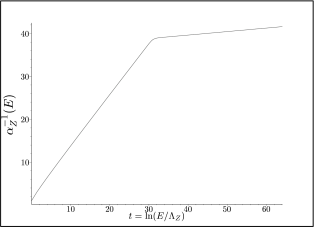
Figure 1: $\alpha_{Z}(E)$ and $\alpha_{Z}^{-1}(E)$ versus $t=\ln(E/\Lambda_{Z})$ for $m_{\tilde{\bm{\varphi}}_{1}^{(Z)}}=300\,GeV$, $m_{\psi^{(Z)}_{2}}=100\;GeV$ and $m_{\psi^{(Z)}_{1}}=50\;GeV$.

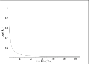
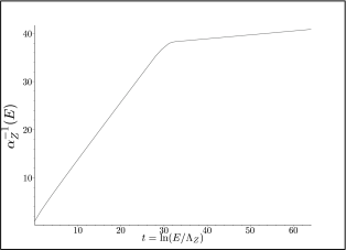
Figure 2: $\alpha_{Z}(E)$ and $\alpha_{Z}^{-1}(E)$ versus $t=\ln(E/\Lambda_{Z})$ for $m_{\tilde{\bm{\varphi}}_{1}^{(Z)}}=300\,GeV$, $m_{\psi^{(Z)}_{2}}=100\;GeV$ and $m_{\psi^{(Z)}_{1}}=10\;GeV$.

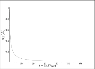
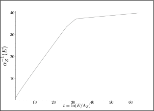
Figure 3: $\alpha_{Z}(E)$ and $\alpha_{Z}^{-1}(E)$ versus $t=\ln(E/\Lambda_{Z})$ for $m_{\tilde{\bm{\varphi}}_{1}^{(Z)}}=300\,GeV$, $m_{\psi^{(Z)}_{2}}=100\;GeV$ and $m_{\psi^{(Z)}_{1}}=1\;GeV$.

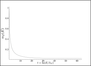
Figure 4: $\alpha_{Z}(E)$ and $\alpha_{Z}^{-1}(E)$ versus $t=\ln(E/\Lambda_{Z})$ for $m_{\tilde{\bm{\varphi}}_{1}^{(Z)}}=300\,GeV$, $m_{\psi^{(Z)}_{2}}=100\;GeV$ and $m_{\psi^{(Z)}_{1}}=1\;MeV$.

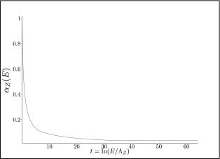
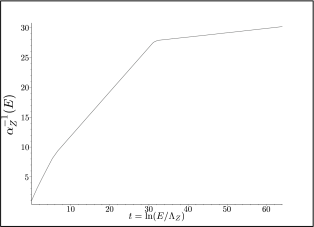
Figure 5: $\alpha_{Z}(E)$ and $\alpha_{Z}^{-1}(E)$ versus $t=\ln(E/\Lambda_{Z})$ for $m_{\tilde{\bm{\varphi}}_{1}^{(Z)}}=300\,GeV$, $m_{\psi^{(Z)}_{2}}=100\;GeV$ and $m_{\psi^{(Z)}_{1}}=1\;eV$.

First we set $m_{\psi^{(Z)}_{2}}=100\;GeV$. We then show in Table I and Figures (1, 2, 3, 4, 5) the dependences of $\alpha_{Z}(M)$ on $m_{\psi^{(Z)}_{1}}$. We show graphs corresponding to $m_{\psi^{(Z)}_{1}}=50\;GeV\,,\,10\;GeV\,,\,1\;GeV\,,\,1\;MeV\,,\,1\;eV$ respectively. We can clearly see that, as we lower the value for $m_{\psi^{(Z)}_{1}}$, $\alpha_{Z}(M)$ also decreases. In fact, $\alpha_{Z}(M)$ varies from $1/41.6$ to $1/30.17$ as $m_{\psi^{(Z)}_{1}}$ varies from $50\,GeV$ to $1\,eV$. From Figs. (1, 2, 3, 4, 5), one notices that $\alpha_{Z}(E)$ and $\alpha_{Z}^{-1}(E)$ are relatively flat until $E$ reaches the mass of the lightest of the two fermions, namely $m_{\psi^{(Z)}_{1}}$. They then steepen and reaches unity at $\Lambda_{Z}=3\times 10^{-3}\,eV$.

Table 1: Correlations between $m_{1}$, $m_{2}$ and $\alpha_{Z}^{-1}(M)$ with $\Lambda_{Z}=3\times 10^{-3}\,eV$ and $M=2\times 10^{16}\,GeV$, for the $SU(2)_{Z}$ triplet and doublet messenger field respectively. The constraint is $\alpha_{Z}(\Lambda_{Z})=1$.

	$m_{1}$	$m_{2}$	$\alpha_{Z}^{-1}(M)$
$m_{\tilde{\bm{\varphi}}_{1}^{(Z)}}=300\,GeV$	$50\,GeV$	$100\,GeV$	$41.6$
	$10\,GeV$	$100\,GeV$	$40.86$
	$1\,GeV$	$100\,GeV$	$39.83$
	$1\,MeV$	$100\,GeV$	$36.7$
	$1\,eV$	$100\,GeV$	$30.17$
	$100\,GeV$	$200\,GeV$	$42.2$
	$50\,GeV$	$200\,GeV$	$41.9$
$m_{\varphi^{(Z)}}=300\,GeV$	$50\,GeV$	$100\,GeV$	$47$

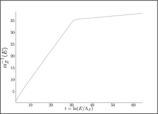
Figure 6: $\alpha_{Z}^{-1}(E)$ versus $t=\ln(E/\Lambda_{Z})$ for $m_{\tilde{\bm{\varphi}}_{1}^{(Z)}}=300\,GeV$, $m_{\psi^{(Z)}_{2}}=100\;GeV$ and $m_{\psi^{(Z)}_{1}}=50\;GeV$ starting with $\alpha_{Z}^{-1}(M)=38$. Here $\alpha_{Z}^{-1}(E=5.7\times 10^{-2}\,eV)=1$.

For the purpose of seeing how e.g. a 10 % change in the initial $\alpha_{Z}(M)$ affects the scale where $\alpha_{Z}$ reaches unity, we show in Fig. (6) $\alpha_{Z}^{-1}(E)$ for the case $m_{\psi^{(Z)}_{1}}=50\;GeV$ with $\alpha_{Z}(M)=1/38$ instead of $1/41.6$ used in Fig. (1) (a 10 % change). We notice that this corresponds to $\Lambda_{Z}^{new}\sim 19\times\Lambda_{Z}\sim 5.7\times 10^{-2}\,eV$, a still very small scale. As we have mentioned above, for a given value of $\alpha_{Z}(M)$, one can always choose $m_{\psi^{(Z)}_{1}}$ so that $\alpha_{Z}=1$ at $\Lambda_{Z}$. (Also, without showing a plot, we find that, for the same set of mass parameters, the choice of $\alpha_{Z}(M)=1/28$, which is a 50 % change from $1/41.6$, will make $\alpha_{Z}=1$ at $\sim 2\times 10^{2}\,eV$.)

For comparison, we also show two plots with $m_{\psi^{(Z)}_{2}}=200\;GeV$ and $m_{\psi^{(Z)}_{1}}=100\;GeV\,,\,50\;GeV$. From Fig. (7, 8), we can see that the change in the initial coupling $\alpha_{Z}(M)$ from the previous case with $m_{\psi^{(Z)}_{2}}=100\;GeV$ and $m_{\psi^{(Z)}_{1}}=50\;GeV$ is insignificant. This is shown in Table I.

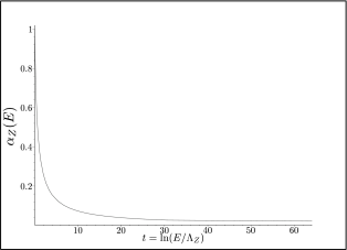
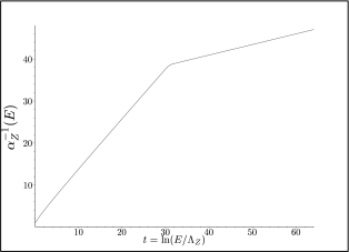
Figure 9: $\alpha_{Z}(E)$ and $\alpha_{Z}^{-1}(E)$ versus $t=\ln(E/\Lambda_{Z})$ for the $SU(2)_{Z}$ doublet case $m_{\bm{\varphi}_{1}^{(Z)}}=300\,GeV$, $m_{\psi^{(Z)}_{2}}=100\;GeV$ and $m_{\psi^{(Z)}_{1}}=50\;GeV$.

Finally, we show in Table I and Fig. (9) a result for the $SU(2)_{Z}$ doublet messenger field. Here we observe that, for the same range of masses, the initial coupling $\alpha_{Z}(M)$ is approximately 11 % smaller than the previous case. As we have mentioned earlier, we will concentrate on the triplet case since it is quite relevant to the SM leptogenesis proposed in our model.

It is interesting to note that the $SU(2)_{Z}$ coupling in various cases shown in Figures (1-9) varies very little from its value at the “GUT” scale $M$ to $E\sim m_{\psi^{(Z)}_{1,2}}$. In this sense, the model is almost scale-invariant in the aforementioned interval. This fact will be very useful in our discussion of candidates in our model of the Cold Dark Matter.

In summary, we have seen in this section that, as can be seen from Table I and Figs. (1-8), it is quite straightforward to have $SU(2)_{Z}$ strongly interacting at a very low mass scale $\Lambda_{Z}=3\times 10^{-3}\,eV$. Furthermore, for initial values of $\alpha_{Z}(M)$ close to the SM couplings at comparable scales- which suggest some unification with the SM at around that scale, the masses of $\psi^{(Z)}_{(L,R),1,2}$ are located in the region (e.g. $\sim 50-200\,GeV$) where the combination of mass values as well as the strength of the $SU(2)_{Z}$ coupling (weak) is such that they can become candidates for the WIMP cold dark matter, a subject to which we will turn below. (We should keep in mind the possibility that $\alpha_{Z}(M)$ can be anywhere in the range shown in Figures (1-8), depending on the mass of $\psi^{(Z)}_{(L,R),1}$ and, furthermore, on the pattern of the GUT breaking as mentioned below.) But we will first discuss the implication of the $SU(2)_{Z}$ scale $\Lambda_{Z}\sim 3\times 10^{-3}\,eV$ concerning the dark energy which is thought to be responsible for the present accelerating universe.

We end this section by briefly mentioning the possibility of unifying $SU(2)_{Z}$ with the SM. The most attractive route in trying to achieve this unification is by noticing that the famous GUT group $E_{6}$ contains $SU(2)\otimes SU(6)$. One can envision the following symmetry breaking chain: $E_{6}\rightarrow SU(2)_{Z}\otimes SU(6)\rightarrow SU(2)_{Z}\otimes SU(3)_{c}\otimes SU(3)_{L}\otimes U(1)\rightarrow SU(3)_{c}\otimes SU(2)_{L}\otimes U(1)_{Y}SU(2)_{Z}\otimes SU(3)_{c}\otimes U(1)_{em}$. A detailed study of this scenario, including the symmetry breaking as well as the evolution of the couplings, is in preparation hung2 .

III $SU(2)_{Z}$ and the Dark Energy

In this section, we will present a scenario in which the $SU(2)_{Z}$ axion is trapped in a false vacuum of an instanton-induced axion potential and whose vacuum energy is $\sim(\Lambda_{Z})^{4}$ su2 . We will then present an estimate of the tunnelling probability to the true vacuum and hence the lifetime of the false vacuum. The basic assumption here is that we are currently living in a false vacuum and that the associated vacuum energy relaxes to zero once the phase transition is completed which will occur in a very, very distant future according to our scenario (see Eq. (39)).

III.1 The axion potential

In Section (II.4), we present a discussion on the spontaneous breakdown of the global $U(1)_{A}^{(Z)}$ symmetry of our model which is responsible for giving masses to $\psi^{(Z)}_{1,2}$. This is due to the non-vanishing VEV of a complex scalar field, $\phi_{Z}=v_{Z}\,\exp(ia_{Z}/v_{Z})+\sigma_{Z}$, where $\langle\sigma_{Z}\rangle=0$ and $\langle a_{Z}\rangle=0$. This results in a massive scalar, $\sigma_{Z}$, and a massless Nambu-Goldstone (NG) boson, $a_{Z}$. (Notice the following periodicity: $a_{Z}\rightarrow a_{Z}+2\pi\,v_{Z}$.) However, the $U(1)_{A}^{(Z)}$ global symmetry is explicitely broken by $SU(2)_{Z}$ instantons and $a_{Z}$ becomes a pseudo Nambu-Goldstone (PNG) boson with a mass squared of order $\Lambda_{Z}^{3}/v_{Z}$ as we shall see below. This is quite similar to the famous Peccei-Quinn axion. This axion, $a_{Z}$, is the “quintessence” field of our model.

The instanton-induced axion potential has been calculated for the PQ axion and can be straightforwardly applied to our model. At zero temperature, one expects the axion potential, in the absence of a soft breaking term, to look like $V(a_{Z})\sim\Lambda_{Z}^{4}[1-\cos\frac{a_{Z}}{v_{Z}}]$ such that $V(a_{Z}=0)=0$. However, at temperatures $T\gg\Lambda_{Z}$, the $SU(2)_{Z}$ axion potential is flat because the contributions from $SU(2)_{Z}$ instantons and anti-instantons are suppressed instanton . In fact, the instanton number density decreases drastically at high temperatures as $n(\rho,T)\propto\exp(-[8\,\pi^{2}/g_{Z}^{2}+c\,(\pi\,\rho\,T)^{2}])$ where $c=2$ when $T>m_{\psi^{(Z)}_{1,2}}$ and $c=4/3$ when $T<m_{\psi^{(Z)}_{1,2}}$, with $\rho$ being the instanton size. Notice also the well-known factor $\exp(-8\,\pi^{2}/g_{Z}^{2})$ which, for an asymptotically free theory like $SU(2)_{Z}$, increases as the temperature decreases since $g_{Z}^{2}$ does so. One might parametrize this phenomenon in the following way:

$$V(a_{Z},T)=\Lambda_{Z}^{4}[1-\kappa(T)\,\cos\frac{a_{Z}}{v_{Z}}]\,,$$ (32)

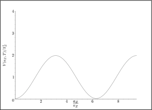
Figure 11: $V(a_{Z},T)/\Lambda_{Z}^{4}$ as a function of $a_{Z}/v_{Z}$ for $\kappa(T)=1$ with no soft breaking.

where $\kappa(T)$ embodies the temperature dependence of the instanton constribution. As we have mentioned earlier, we expect $\kappa(T)$ to rapidly decrease in magnitude as $T\gg\Lambda_{Z}$ and, as a result, $V(a_{Z},T\gg\Lambda_{Z})\sim\Lambda_{Z}^{4}$. However, for $T\leq\Lambda_{Z}$, one also expects $\kappa(T)\sim 1$ in which case $V(a_{Z},T)$ exhibits two degenerate minima, one at $\langle a_{Z}\rangle=0$ and one at $\langle a_{Z}\rangle=2\pi v_{Z}$, with the potential barrier between the two being $2\,\Lambda_{Z}^{4}$. This is due to the fact that there is a remaining $Z(2)$ symmetry. Such degeneracy is well-known in the PQ axion potential as it has been noted by sikivie . The computation of $\kappa(T)$ is fairly model-dependent. For our purposes, we only need to require that $\kappa(T)\rightarrow 0$ for $T\gg\Lambda_{Z}$ and $\kappa(T)\sim 1$ for $T\leq\Lambda_{Z}$, noting that calculations for the integrated instanton density at high temperatures as used in the effective PQ axion potential show that it falls as $T^{-8}$. In Figures (10,11), we show $V(a_{Z},T)$ for two values of $\kappa(T)$: $\kappa(T)=1$ and $\kappa(T)=10^{-3}$ (as an illustrative value). Notice how quickly $V(a_{Z},T)$ quickly flattens out at high temperature. (For that reason, we do not show figures with $\kappa(T)<10^{-3}$.)

In sikivie , the $Z(N)$ degeneracy of the PQ axion potential is lifted by a soft-breaking term (to evade the so-called domain wall problem) of the form $e^{i\delta}\,\mu^{3}\Phi+h.c.$, where $\Phi$ is a SM singlet and $\mu^{3}\ll\Lambda_{QCD}^{4}/v_{\Phi}$. Similarly, as in su2 , we would like to propose the following $U(1)_{A}^{(Z)}$ soft breaking term to lift the $Z(2)$ degeneracy:

$$V_{B}=\Lambda_{Z}^{4}\,\frac{a_{Z}}{2\pi\,v_{Z}}\,.$$ (33)

We shall assume a similar temperature dependence namely $\kappa(T)$ for $V_{B}$ such that for $T\gg\Lambda_{Z}$, the total effective potential $V_{tot}=V(a_{Z},T)+V_{B}(T)$ is flat and, for $T\leq\Lambda_{Z}$ where we assume that $\kappa(T)=1$, it is given by $V_{tot}=\Lambda_{Z}^{4}[1-\cos\frac{a_{Z}}{v_{Z}}]+\Lambda_{Z}^{4}\,\frac{a_{Z}}{2\pi\,v_{Z}}$. We propose

$$V_{tot}(a_{Z},T)=\Lambda_{Z}^{4}[1-\kappa(T)\,\cos\frac{a_{Z}}{v_{Z}}]+\kappa(T)\Lambda_{Z}^{4}\,\frac{a_{Z}}{2\pi\,v_{Z}}\,.$$ (34)

III.2 The false vacuum, its transition probability and the equation of state

We now discuss a cosmological scenario based on (34).

1) We show in Figure (12) $V_{tot}(a_{Z},T)$ for $\kappa(T)=10^{-3}$. So, at $T\gg\Lambda_{Z}$, the potential is flat. One might expect the value of the classical $a_{Z}$ field to be $a_{Z}\sim O(v_{Z})$. As long as the potential stays flat, it will hover around that value as the temperature decreases.

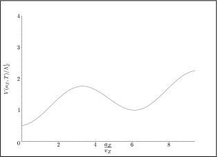
Figure 13: $V(a_{Z},T)/\Lambda_{Z}^{4}$ as a function of $a_{Z}/v_{Z}$ for $\kappa(T)=10^{-0.3}$ with soft breaking.

2) We show in Figure (13) $V_{tot}(a_{Z},T)$ for $\kappa(T)=10^{-0.3}$. We now see the appearance of two local minima: one at $a_{Z}=0$ and the other (higher in energy) at $a_{Z}=2\,\pi\,v_{Z}$. The latter is the false vacuum that we had mentioned above. As $a_{Z}$ hovers around $\sim O(v_{Z})$ when the temperature decreases, it gets trapped in the false vacuum when a local minimum develops at $a_{Z}=2\,\pi\,v_{Z}$.

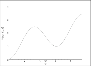
Figure 14: $V(a_{Z},T)/\Lambda_{Z}^{4}$ as a function of $a_{Z}/v_{Z}$ for $\kappa(T)=1$ with soft breaking.

3) In Figure (14), we show $V_{tot}(a_{Z},T)$ for $\kappa(T)=1$, i.e. at $T\sim\Lambda_{Z}$. The true vacuum at $a_{Z}=0$ now has zero energy density and the barrier between the two vacuua is now higher. The difference in energy density between the true vacuum at $a_{Z}=0$ and the false vacuum at $a_{Z}=2\,\pi\,v_{Z}$ is $\Lambda_{Z}^{4}$. The universe is still trapped in the false vacuum. How long does it stay there?

The first order phase transition to the true vacuum at $a_{Z}=0$ proceeds by bubble nucleation. The rate of the nucleation of the true vacuum bubble is written as

$$\Gamma=A\exp\{-S_{E}\}\,,$$ (35)

where the Euclidean action $S_{E}$, in the thin wall limit, can be computed by looking at

$$\tilde{S}=\int_{a_{Z}=2\pi v_{Z}}^{a_{Z}=0}\sqrt{2(\Lambda_{Z}^{4})[1-\cos\frac{a_{Z}}{v}]}da_{Z}=8\,v_{Z}\;\Lambda_{Z}^{2}$$ (36)

giving

$$S_{E}=\frac{27\,\pi^{2}\,\tilde{S}^{4}}{2\,\Lambda_{Z}^{12}}\geq 5\times 10^{5}\,(\frac{v_{Z}}{\Lambda_{Z}})^{4}\,.$$ (37)

For $v_{Z}\sim$ a few hundreds of GeVs, the lower bound on $S_{E}$ is huge, approximately $10^{62}$! The transition time can be estimated to be (with $T_{c}\sim\Lambda_{Z}$)

$$\tau=\frac{3\,H}{4\,\pi\Gamma}\sim\{(\frac{\Lambda_{Z}}{m_{pl}})^{2}\exp\{S_{E}\}\}\,t_{pl}\,,$$ (38)

where we have taken $H\sim T_{c}^{2}/m_{pl}$ and $A\sim O(1)$. This gives an estimate for the transition time to be approximately

$$\tau\geq(10^{-106}\,s)\exp(10^{62})\,.$$ (39)

A value of $\tau$ of this magnitude means that practically one is stuck in the false vacuum for a very, very long time.

Assuming $a_{Z}$ to be spatially uniform, the equation of state parameter $w$ is given by the well-known expression

$$w(a_{Z})=\frac{\frac{1}{2}\dot{a}_{Z}^{2}-V(a_{Z})}{\frac{1}{2}\dot{a}_{Z}^{2}+V(a_{Z})}\,.$$ (40)

When the universe is trapped in the false vacuum at $a_{Z}=2\pi v_{Z}$, $\frac{1}{2}\dot{a}_{Z}^{2}\sim 0$ and one obtains

$$w(a_{Z})\approx-1\,.$$ (41)

This means that the quintessence scenario presented here effectively mimics the flat $\Lambda\,CDM$ model!

III.3 Estimates of various ages of the universe in our scenario

It is useful to estimate when the energy density ,$\Lambda_{Z}^{4}$, of the false vacuum started to dominate over the matter (baryonic and non-baryonic) energy density and when the deceleration ceased and the acceleration kicked in. First, one can readily estimate the temperature and time when $\rho_{vac}=\Lambda_{Z}^{4}$ equals the matter (baryonic and non-baryonic) energy density $\rho_{M}$ as follows. We start with the now accepted flat universe condition

$$\Omega_{M}+\Omega_{\Lambda_{Z}}=1\,,$$ (42)

where for definiteness we set the present values of $\Omega$’s to be

$$\Omega_{M}^{0}=0.3\;;\;\Omega_{\Lambda_{Z}}^{0}=0.7\,.$$ (43)

Since $\rho_{M}\propto T^{3}$ and $\rho_{vac}=\Lambda_{Z}^{4}$ is constant, it follows that, with $T_{0}=2.7^{0}\,K$,

$$T=T_{0}\,(\frac{0.7}{0.3})^{1/3}\,(\frac{\rho_{M}(T)}{\rho_{vac}})^{1/3}\,.$$ (44)

From (44), the temperature $T_{eq}$ at which $\rho_{M}(T_{eq})=\rho_{vac}$ is found to be

$$T_{eq}\approx 3.6^{0}\,K\,.$$ (45)

In terms of the redshift variable $z$, since $\rho_{M}\propto(1+z)^{3}$, one finds

$$z_{eq}=(\frac{0.7}{0.3})^{1/3}-1\approx 0.33\,.$$ (46)

The age of the universe at a given redshift value $z$ is given by

$$t(z)=H_{0}^{-1}\int_{z}^{\inf}\frac{dz^{{}^{\prime}}}{(1+z^{{}^{\prime}})[\Omega_{M}(1+z^{{}^{\prime}})^{3}+\Omega_{vac}]^{1/2}}\,,$$ (47)

where $H_{0}^{-1}=(0.96\pm 0.04)^{-1}\,t_{0}$ with $t_{0}=13\pm 1.5Gyr$ being the present age of the universe. Using Eq. (47), we obtain the following age when the equality happened:

$$t_{eq}=9.5\pm 1.1\,Gyr\,.$$ (48)

One may also want to know at what value of $z$ the deceleration “stopped” and the acceleration “started”. With the equation for the cosmic scale factor $a(t)$ being

$$\frac{\ddot{a}}{a}=-\frac{4\pi\,G}{3}\sum_{i}\rho_{i}(1+3\,w_{i})\,,$$ (49)

with $w_{M}=0$ and $w_{vac}=-1$, the transition between the two regimes occured when $\ddot{a}=0$, giving

$$\rho_{M}(z_{a})-2\,\rho_{vac}=0\,.$$ (50)

This gives

$$z_{a}=(\frac{2\times 0.7}{0.3})^{1/3}-1\approx 0.67\,.$$ (51)

The corresponding time and temperature are

$$t_{a}\approx 7.2\pm 0.8\,Gyr\,,$$ (52)

$$T_{a}\approx 4.5^{0}K\,.$$ (53)

The previous exercises serve two purposes: they give an estimate of the time, temperature and redshift value of the period when the vacuum energy density began to dominate over the matter energy density and the same quantities for the period when the universe changed from a deceleration stage to an accelerating one, and to compare the two. As one can see, the acceleration began, in this scenario, about two billion years before the dominance of the vacuum energy density. As it is well-known, both events occured rather “recently”.

The next question is the temperature, time and redshift value of the epoch when the axion potential developed a false local minimum, i.e.when $T_{Z}\sim\Lambda_{Z}$. One has to be however a little bit more careful here concerning the temperature of the $SU(2)_{Z}$ plasma as compared with that of the SM plasma. At $T\gg m_{i}$, where $m_{i}$ is a generic particle mass, all normal matter and matter that carries $SU(2)_{Z}$ quantum numbers are in thermal equilibrium and are characterized by a common temperature $T$. The fact that $SU(2)_{Z}$ matter is in thermal equilibrium with normal matter is because the messenger fields, ${\tilde{\bm{\varphi}}}_{i}^{(Z)}$ or $\varphi^{(Z)}$, carry both SM and $SU(2)_{Z}$ quantum numbers and, therefore, can interact with normal matter as well as with the $SU(2)_{Z}$ “gluons” and fermions $\psi^{(Z)}$. In what follows we will concentrate on the scenario with ${\tilde{\bm{\varphi}}}_{i}^{(Z)}$ and the estimates to be made below can be easily made for the $\varphi^{(Z)}$ case.

We first show that the energy density of the $SU(2)_{Z}$ plasma at the time of Big Bang Nucleosynthesis (BBN) is a small fraction of the SM plasma energy density. As a consequence, it does not affect BBN. We then relate the temperatures of the two plasmas when the lightest of the two $\psi^{(Z)}$’s drops out of thermal equilibrium.

When $T<m_{\tilde{\bm{\varphi}}^{(Z)}}$, ${\tilde{\bm{\varphi}}}_{1}^{(Z)}$ drops out of thermal equilibrium (how much might remain will be the subject of the next section), $SU(2)_{Z}$ “gluons” and fermions $\psi^{(Z)}$ practically decouple from the SM plasma and its temperature $T_{Z}$ would go like $R^{-1}$. To find its relationship with the SM temperature $T$, we use the familiar expression for the effective number of relativistic degrees of freedom $g_{\ast}=\sum g_{bosons}+(7/8)\sum g_{fermions}$. Let us recall that $g_{\ast}$ for the SM above the top quark mass is $g_{\ast}^{SM}=427/4$ (right-handed neutrinos are not counted, being SM singlets). To this we add the contibution from the $SU(2)_{Z}$ sector when all particles are in thermal equilibrium. So for $T>m_{\tilde{\bm{\varphi}}^{(Z)}}$, we obtain $g_{\ast}^{SU(2)_{Z}}=39$ giving

$$g_{\ast}^{total}=\frac{583}{4}\,.$$ (54)

After ${\tilde{\bm{\varphi}}}_{1}^{(Z)}$ decouples, let us, for definiteness, label the temperature of the SM plasma by $T$ and that of the $SU(2)_{Z}$ plasma by $T_{Z}$. The SM number of degrees of freedom for $m_{e}<T<m_{\mu}$ is $g_{\ast}^{SM}=43/4$. Furthermore, if the mass of the lightest of the two $\psi^{(Z)}$’s, namely $\psi^{(Z)}_{1}$, is of O(GeV) as we had discussed in Section (II.6), the effective number of $SU(2)_{Z}$ degrees of freedom after $\psi^{(Z)}_{1}$ decoupling is simply $g_{\ast}^{SU(2)_{Z}}=6$, while it is $g_{\ast}^{SU(2)_{Z}}=27$ after ${\tilde{\bm{\varphi}}}_{1}^{(Z)}$ decoupling. One obtains

$$T_{Z}=(\frac{27}{6}\,\frac{43}{583})^{1/3}\,T\approx 0.7\,T\,.$$ (55)

This gives

$$\frac{\rho_{SU(2)_{Z}}}{\rho_{SM}}=(6\times\frac{4}{43})\times(\frac{27}{6}\,\frac{43}{583})^{4/3}\approx 0.13\,.$$ (56)

From Eq. (56), one can see that BBN is not affected by the presence of the $SU(2)_{Z}$ plasma.

One can also relate $T_{Z}$ to the CMB temperature after $e^{\pm}$ decoupling, i.e. for $T<m_{e}$. (This is very similar to the relation between the photon and neutrino temperatures.) It is given by

$$T_{Z}=(\frac{27}{6}\,\frac{43}{583}\,\frac{4}{11})^{1/3}\,T\approx 0.5\,T\,.$$ (57)

The $SU(2)_{Z}$ coupling grows strong ($\alpha_{Z}=1$) at $T_{Z}\sim 3\times 10^{-3}\,eV\sim 35^{0}K$. Using Eq. (57), one can estimate the photon temperature at that point to be

$$T\approx 70^{0}K\,.$$ (58)

This corresponds to a redshift

$$z\approx 25\,.$$ (59)

The age of the universe at that point can be calculated using Eq. (47) to give

$$t_{z}\approx 125\pm 14Myr\,.$$ (60)

We now summarize the different epochs by listing the triplets of numbers: redshift, age, and photon temperature. They are:

a) ($z\approx 25,t_{z}\approx 125\pm 14Myr,T\approx 70^{0}K$) when $SU(2)_{Z}$ grew strong;

b) ($z_{a}\approx 0.67,t_{a}\approx 7.2\pm 0.8Gyr,T\approx 4.5^{0}K$) when the acceleration “kicked in”;

c) ($z_{eq}\approx 0.33,t_{eq}\approx 9.5.\pm 1.1Gyr,T\approx 3.6^{0}K$) when the energy density of the false vacuum equals that of (baryonic and non-baryonic) matter.

From this summary, several remarks are in order.

1) According to our scenario, the universe got trapped in the false vacuum of the $a_{Z}$ potential long before it began to accelerate. This means that the mechanism which gives rise to the acceleration seven billion years later occured at an age when the false vacuum energy density was completely negligible compared with the matter energy density.

2) The fact that it started to accelerate six billion years ago (i.e. relatively recent time) and that the dark energy density is comparable to that of matter has to do with the magnitude of the false vacuum energy density $\rho_{vac}\sim(3\times 10^{-3}\,eV)^{4}$. This is generic with any $\Lambda\,CDM$ model having that value of vacuum energy density. Heuristically speaking, if a model can generate a scale this low (i.e.at such a low temperature), the acceleration process as well as the similarity in magnitudes of energy densities necessarily took place fairly “recently”.

3) This so-called coincidence (“why now”) problem is related to that particular value of false vacuum energy density. In our scenario, this comes from the scale $\sim 10^{-3}\,eV$ where $SU(2)_{Z}$ grows strong as we have discussed in Section (II.6). In that section, the initial value of the $SU(2)_{Z}$ gauge coupling at some “GUT” scale of the order of $10^{16}\,GeV$ is taken to be comparable to that of a SM coupling at a comparable scale. This is possible if $SU(2)_{Z}$ were to merge with the SM into some grand unified group. There is indeed one of such groups: the well-known $E_{6}$. One can envision the following symmetry breaking pattern down to the SM: $E_{6}\rightarrow SU(2)_{Z}\otimes SU(6)\rightarrow SU(2)_{Z}\otimes SU(3)_{c}\otimes SU(3)_{L}\otimes U(1)_{1}\rightarrow SU(2)_{Z}\otimes SU(3)_{c}\otimes SU(2)_{L}\otimes U(1)_{2}\otimes U(1)_{1}\rightarrow SU(2)_{Z}\otimes SU(3)_{c}\otimes SU(2)_{L}\otimes U(1)_{Y}$. This path of $E_{6}$ breaking is very different from the usual one where $E_{6}\rightarrow SO(10)$. (The details of this scenario will appear elsewhere hung2 .) From this pattern, one notices the following features: (i) the $SU(2)_{Z}$ and $SU(6)$ couplings are equal at the scale of $E_{6}$ breaking which implies that the $SU(2)_{Z}$ coupling is close to but does not have to be equal to the SM couplings at the same scale; (ii) the unification of the SM itself follows a different route from the conventional one where 3-2-1 merge into $SU(5)$ or $SO(10)$.

Based on the arguments presented above, one cannot help, within the context of our model, but wonder if the dark energy might be a direct remnant of the unification scenario discussed above. It is often said that there appears to be an “indirect evidence” for Grand Unification in the form of supersymmetric (SUSY) $SU(5)$ or $SO(10)$ by “running” the three SM couplings and finding that they all meet at one point around $10^{16}\,GeV$. However, considering the possibility that the path to unification can be more complicated than SUSY $SU(5)$ or $SO(10)$, this “indirect evidence” based on the meeting of the three SM couplings might be taken with caution. Perhaps the dark energy, or equivalently the accelerating universe, could be the first “direct evidence” of Grand Unification?

III.4 The mass of the quintessence axion field $a_{Z}$

The last topic that we would like to discuss in this section is the mass of the axion field $a_{Z}$. As we mentioned above, $a_{Z}$ would be a massless NG boson if it were not for the fact that the global $U(1)_{A}^{(Z)}$ symmetry is explicitely broken by $SU(2)_{Z}$ instantons. It then acquires a mass which can be computed in a similar fashion to that for the PQ axion in QCD sikivie2 .

The mass of $a_{Z}$ can be computed by taking the vacuum expectation value of the term $\sum_{i}K_{i}\,\bar{\psi}^{(Z)}_{L,i}\,\psi^{(Z)}_{R,i}\,\phi_{Z}+h.c.$ in Eq. (5). From

$$\langle\sum_{i}|K_{i}|\,\bar{\psi}^{(Z)}_{L,i}\,\psi^{(Z)}_{R,i}\,\phi_{Z}+H.c.\rangle=2\,\sum_{i}|K_{i}|\,\mu_{i}^{3}\,v_{Z}\,\cos(\frac{a_{Z}}{v_{Z}})\,,$$ (61)

and $\langle\bar{\psi}^{(Z)}_{L,i}\,\psi^{(Z)}_{R,i}\rangle=\mu_{i}^{3}$ one obtains the following mass squared for $a_{Z}$

$$m_{a_{Z}}^{2}=\frac{2\,\sum_{i}|K_{i}|\,\mu_{i}^{3}}{v_{Z}}\,.$$ (62)

An approximate estimate of the upper bound of $m_{a_{Z}}$ can be found by setting $\mu_{i}^{3}\sim\Lambda_{Z}^{3}$ and $\sum_{i}|K_{i}|\lesssim 1$ in (62) giving

$$m_{a_{Z}}\lesssim\Lambda_{Z}\,\sqrt{\frac{2\,\Lambda_{Z}}{v_{Z}}}\sim 10^{-10}\,eV\,,$$ (63)

where we have set $v_{Z}\sim 300\,GeV$ for simplicity. In fact, if we do not want $K_{i}$ to be too much smaller than unity and since at least $m_{\psi^{(Z)}_{2}}\sim\mathcal{O}(100\,GeV)$, that choice is reasonable for $v_{Z}$.

From Eq. (5), one can write down the interaction term between $a_{Z}$ and the $SU(2)_{Z}$ fermions as follows

$${\cal L}_{a_{Z}}=i(\sum_{i}(\frac{m_{\psi^{(Z)}_{i}}}{v_{Z}})\bar{\psi}^{(Z)}_{i}\,\gamma_{5}\psi^{(Z)}_{i})\,a_{Z}\,.$$ (64)

For $m_{a_{Z}}\sim 10^{-10}\,eV$, the range of interaction between two $\psi^{(Z)}$s is approximately $1\,km$. The astrophysical implication of this interaction is under investigation.

We now turn our attention to two other cosmological implications of our model: candidates for the Weakly Interacting Massive particles (WIMP) form of Cold Dark Matter (CDM), and a mechanism for leptogenesis. The latter (leptogenesis) topic will appear as a companion paper while the former (CDM) topic is under investigation. For this reason, the presentations which follow will be brief.

IV $\psi^{(Z)}_{1,2}$ as candidates for Cold Dark Matter

In this section, we will present a heuristic argument suggesting that the $SU(2)_{Z}$ fermions $\psi^{(Z)}_{1,2}$ could be candidates for the cold dark matter, keeping in mind that the dark matter might very well consist of a mixture of different particles.

As we have discussed above, at high temperatures $\psi^{(Z)}_{1,2}$ are in thermal equilibrium with the $SU(2)_{Z}$ plasma as well as with the SM plasma because of the presence of a messenger scalar field which, for definiteness, we will take to be ${\tilde{\bm{\varphi}}}_{1}^{(Z)}$.

In principle, our scenario could contain several “candidates” for CDM: ${\tilde{\bm{\varphi}}}_{1}^{(Z)}$ and $\psi^{(Z)}_{1,2}$. As $T$ drops below various mass thresholds of these particles, they will start the annihilation process that reduces their number. Out of the three, ${\tilde{\bm{\varphi}}}_{1}^{(Z)}$ would be the most unstable particle. In the next section, we will show that its decay which is constrained to occur at a temperature $T_{D}$ larger that the electroweak temperature $T_{EW}\sim 100\,GeV$ gives rise to a SM lepton asymmetry which is reprocessed into a baryon asymmetry through the electroweak sphaleron process. In what follows, we will only consider $\psi^{(Z)}_{1,2}$ as possible CDM candidates.

Since we assume $m_{{\tilde{\bm{\varphi}}}_{1}^{(Z)}}>m_{\psi^{(Z)}_{2}}>m_{\psi^{(Z)}_{1}}$, it is obvious that $\psi^{(Z)}_{1}$ is stable. From (5), one can see that $\psi^{(Z)}_{2}$ can decay into $\psi^{(Z)}_{1}+{\bf A}^{(Z)}$ via a one-loop diagram. A rough estimate of the decay rate of $\psi^{(Z)}_{2}$ gives $\Gamma_{\psi^{(Z)}_{2}}\sim(\alpha_{{\tilde{\varphi}_{1}}^{1}}\alpha_{{\tilde{\varphi}_{1}}^{2}}\,\alpha_{Z})\,m_{\psi^{(Z)}_{2}}$ which could be less than the Hubble rate if the Yukawa couplings in (5) are small enough. Furthermore, if the Yukawa couplings are sufficiently small so that the interactions freeze out before it decays, $\psi^{(Z)}_{2}$ could be considered to be stable. When $T<m_{\psi^{(Z)}_{2}}$, the number density of $\psi^{(Z)}_{2}$ decreases like $exp(-m/T)$ until its annihilation rate drops below the Hubble rate and $\psi^{(Z)}_{2}$ drops out of thermal equilibrium. To find out about the relic abundance of $\psi^{(Z)}_{2}$ and of $\psi^{(Z)}_{1}$, one needs to know the size of the annihilation cross sections.

One of the most attractive candidates for CDM is a stable particle which has an annihilation cross section typically the size of the electroweak cross section. Although a detailed analysis is needed in order to make a more precise prediction, an insight can be gained in this section by noticing that an approximate solution to the Boltzmann equation gives the following estimate for the fraction of the energy density coming from the relic abundance kamionkowski

$$\Omega_{\psi^{(Z)}_{2}}=\frac{m_{\psi^{(Z)}_{2}}\,n_{\psi^{(Z)}_{2}}}{\rho_{c}\,h^{2}}\approx\bigl{(}\frac{3\times 10^{-27}\,cm^{3}\,sec^{-1}}{\langle\sigma_{A,\psi^{(Z)}_{2}}\,v\rangle}\bigr{)}\,,$$ (65)

where $\rho_{c}=3\,H^{2}/8\,\pi\,G$ is the critical density, $h\approx 0.72$ and $\sigma_{A,\psi^{(Z)}_{2}}$ is the annihilation cross section for $\sigma_{A,\psi^{(Z)}_{2}}$. In this approximation, (65) is independent of the $\psi^{(Z)}_{2}$ mass and depends only on its annihilation cross section kamionkowski . For this reason and using the same approximation, we infer that

$$\Omega_{\psi^{(Z)}_{1}}=\frac{m_{\psi^{(Z)}_{1}}\,n_{\psi^{(Z)}_{1}}}{\rho_{c}\,h^{2}}\approx\bigl{(}\frac{3\times 10^{-27}\,cm^{3}\,sec^{-1}}{\langle\sigma_{A,\psi^{(Z)}_{1}}\,v\rangle}\bigr{)}\,.$$ (66)

In order for $\Omega_{\psi^{(Z)}_{2}}$ and/or $\Omega_{\psi^{(Z)}_{1}}$ or $\Omega_{\psi^{(Z)}_{2}}+\Omega_{\psi^{(Z)}_{1}}$ to be of order unity, the annihilation cross sections $\sigma_{A,\psi^{(Z)}_{1,2}}$ should have a magnitude of the order $3\times 10^{-27}\,cm^{3}\,sec^{-1}/\langle v\rangle$. Although $\psi^{(Z)}_{1,2}$ are non-relativistic when $T$ drops below their masses, $\langle v\rangle$ might not be too small. For the sake of estimate, let us assume $\langle v\rangle\sim 0.1\,c$. A typical magnitude for the annihilation cross sections so that the relic abundance of CDM is of the right order would be

$$\langle\sigma_{A,\psi^{(Z)}_{1,2}}\rangle\sim 10^{-36}\,cm^{2}\sim\frac{3\times 10^{-9}}{GeV^{2}}\,.$$ (67)

Under what conditions would $\sigma_{A,\psi^{(Z)}_{1,2}}$ have a magnitude $\sim 10^{-36}\,cm^{2}\sim\frac{3\times 10^{-9}}{GeV^{2}}$? In our model, the dominant annihilation cross section goes like

$$\sigma_{A,\psi^{(Z)}}\sim\frac{\alpha_{Z}(T)^{2}}{T^{2}}\,,$$ (68)

for $T<m_{\psi^{(Z)}}$. From Fig. (1, 2, 3, 4, 5), we can see that $\alpha_{Z}(T)$ is relatively “flat” for a large range of energy, ranging from $\sim 10^{16}\,GeV$ down to approximately $m_{\psi^{(Z)}_{2}}$ where it begins to “rapidly” increase. We also see that this “flat” value for $\alpha_{Z}(T)$ depends on the mass of $\psi^{(Z)}_{1}$ for $m_{\psi^{(Z)}_{2}}\sim\mathcal{O}(100\,GeV)$. Typically, $\alpha_{Z}(T)\sim 1/30-1/40$ for $m_{\psi^{(Z)}_{1}}\sim 1\,eV-50\,GeV$ according to Fig. (1, 2, 3, 4, 5). We can now make two generic remarks.

1) From (68) and from $\alpha_{Z}(T)^{2}\sim 6\times 10^{-4}$, one can infer that $T<m_{\psi^{(Z)}}<1\,TeV$ otherwise $\psi^{(Z)}$ will become overabundant.

2) $\psi^{(Z)}_{1}$ cannot be too light e.g. $<10\,GeV$ or so since this would lead to a cross section which could be too large and which could greatly reduce its relic abundance. Therefore,if it were to be a CDM candidate, its mass should be high enough in value in order for the cross section to be of the right order of magnitude since $\alpha_{Z}(T)^{2}$ is practically “constant” in the interval of interest.

The above discussion makes clear that, whether or not $\psi^{(Z)}_{1,2}$ can be considered to be reasonable WIMP CDMs, it is a question which actually depends on the masses of these particles through the magnitude of their annihilation cross sections. Furthermore, the best range of masses appears to be of $\mathcal{O}(100-1000\,GeV)$. It is interesting to note the following fact. As we have seen in Section (II.6), this range of masses for both $\psi^{(Z)}_{1}$ and $\psi^{(Z)}_{2}$ gives a value for the initial $SU(2)_{Z}$ coupling $\alpha_{Z}(M)$ $\sim 1/42$ which is very close to the (non-supersymmetric) SM couplings at a similar scale, which suggests some kind of unification as we had mentioned earlier. (A full investigation of the unification issue is slightly more complicated.) The next question is the following: Which of the $\psi^{(Z)}$s is the best candidate or is it both? Below we list two possible scenarios with one being more attractive than the other.

• $m_{\psi^{(Z)}_{2}}\sim\mathcal{O}(100\,GeV)$, $m_{\psi^{(Z)}_{1}}\sim\mathcal{O}(<10\,GeV)$:

  Here it is unlikely for $\psi^{(Z)}_{1}$ to be a WIMP because of its mass but $\psi^{(Z)}_{2}$ could. However, as we have noted above, $\psi^{(Z)}_{2}$ decays into $\psi^{(Z)}_{1}+{\bf A}^{(Z)}$. The decay rate which arises at one loop depends very much on the strength of the Yukawa couplings in (5), in particular the one involving $\psi^{(Z)}_{1}$ . The decay rate of $\psi^{(Z)}_{2}$ is approximately $\Gamma_{\psi^{(Z)}_{2}}\sim(\alpha_{Z}\,\alpha_{{\tilde{\bm{\varphi}}}_{1}^{(Z)}}\,\alpha_{{\tilde{\bm{\varphi}}}_{2}^{(Z)}})(m_{\psi^{(Z)}_{2}}/m_{{\tilde{\bm{\varphi}}}_{1}^{(Z)}})^{4}(m_{\psi^{(Z)}_{2}}/16\,\pi^{2})$. For $m_{\psi^{(Z)}_{2}}\sim\mathcal{O}(m_{{\tilde{\bm{\varphi}}}_{1}^{(Z)}})$, one notices that $\psi^{(Z)}_{2}$ can only survives until the present time ($\sim 4.3\times 10^{17}\,sec$ if $\alpha_{{\tilde{\bm{\varphi}}}_{1}^{(Z)}}\,\alpha_{{\tilde{\bm{\varphi}}}_{2}^{(Z)}}\sim 10^{-41}$ which might be quite unnatural. Otherwise $\psi^{(Z)}_{2}$ will decay out-of-equilibrium at some earlier times. Whether or not the decay process preserves the desired fraction of the total energy density is beyond the scope of this paper and will be presented elsewhere.

• $m_{\psi^{(Z)}_{2}}\sim m_{\psi^{(Z)}_{1}}\sim\mathcal{O}(100\,GeV)$, e.g. $m_{\psi^{(Z)}_{2}}=200\,GeV$ and $m_{\psi^{(Z)}_{1}}=100\,GeV$ as shown in Fig. (7):

  This case appears to be the more desirable one. The lighter of the two and hence the stable one, namely $\psi^{(Z)}_{1}$, has a mass of $\mathcal{O}(100\,GeV)$ and, from the results of the above discussion, can have the desired relic abundance. Alternatively, a combination of $\psi^{(Z)}_{1}$ and $\psi^{(Z)}_{2}$ (or its decay product) can have the desired abundance. Since $\psi^{(Z)}_{2}$ decays, the principal WIMP candidate is actually $\psi^{(Z)}_{1}$.

One last remark we would like to make in this section concerns the present form of the WIMP candidate(s) of our model. As we discuss above, $SU(2)_{Z}$ grows strong at $\Lambda_{Z}\sim 10^{-3}\,eV$. If we assume that this leads to confinement as with QCD, the $SU(2)_{Z}$ singlets would be a spin zero composite of two $\psi^{(Z)}$s. In priciple, one would also have a spin one-half composite of one $\psi^{(Z)}$ and a messenger field. However, the messenger field decays and practically disappears long before this “confinement” occurs. Therefore, the present form of WIMP in our model would be a chargeless, spin zero $SU(2)_{Z}$ “hadron” whose phenomenological implication is briefly discussed in Section (VI). Presumably the size of this “hadron” would be of the order $\hbar c/10^{-3}\,eV\sim 1\,mm$ which is rather large.

V $SU(2)_{Z}$ and leptogenesis

In this section, we will present a brief discussion of the possibility of leptogenesis in our model. A full presentation will appear in a companion article.

As we have presented above, our model contains two $SU(2)_{Z}$ triplet complex scalar fields, $\tilde{\bm{\varphi}}_{1}^{(Z)}$ and $\tilde{\bm{\varphi}}_{2}^{(Z)}$. These fields interact with $\psi^{(Z)}_{1,2}$ and the SM leptons via Eq. (5). In Section (II.6), one of the two messenger fields, $\tilde{\bm{\varphi}}_{2}^{(Z)}$, was set to have a large mass of the order of the “GUT” scale and the evolution of the $SU(2)_{Z}$ coupling on the messenger fields depends only on $\tilde{\bm{\varphi}}_{1}^{(Z)}$ as well as on the $SU(2)_{Z}$ fermions. $\tilde{\bm{\varphi}}_{1}^{(Z)}$ can decay into $\psi^{(Z)}_{1,2}$ plus a SM lepton. The interference between the tree-level and one-loop amplitude for the previous decay generates a SM lepton number violation which transmogrifies into a baryon asymmetry through the electroweak sphaleron process kuzmin , lepto . An important point to keep in mind is the fact that $\psi^{(Z)}_{1,2}$ are SM singlets and the $\psi^{(Z)}_{1,2}$ number violation cannot be reprocessed by the electroweak sphaleron. So the rule of thumb here is the following: SM lepton number violation $\rightarrow$ quark (or baryon) number violation.

$\tilde{\bm{\varphi}}_{1}^{(Z)}$ is in thermal equilibrium (with the $SU(2)_{Z}$ as well as with the SM plasmas) at $T>m_{{\tilde{\bm{\varphi}}}_{1}^{(Z)}}$. When $T\approx m_{{\tilde{\bm{\varphi}}}_{1}^{(Z)}}$, one would like $\tilde{\bm{\varphi}}_{1}^{(Z)}$ to decouple before it decays. The primary condition for a departure from thermal equilibrium is the requirement that the decay rate $\Gamma_{{\tilde{\bm{\varphi}}}_{1}^{(Z)}}\sim\alpha_{\tilde{\varphi}_{1}}m_{\tilde{\varphi}_{1}}$, with $\alpha_{\tilde{\varphi}_{1}}=g_{\alpha_{\tilde{\varphi}_{1}}}^{2}/4\pi$, is less than the expansion rate $H=1.66\,g_{*}^{1/2}T^{2}/m_{pl}$, where $g_{*}$ is the effective number of degrees of freedom at temperature $T$. As with kolb , we can define

$$K\equiv(\Gamma_{\tilde{\varphi}_{1}}/2\,H)_{T=m_{\tilde{\varphi}_{1}}}=\frac{\alpha_{\tilde{\varphi}_{1}}\,m_{pl}}{3.3\,g_{*}^{1/2}\,m_{{\tilde{\bm{\varphi}}}_{1}^{(Z)}}}\,.$$ (69)

When $K\ll 1$, $\tilde{\bm{\varphi}}_{1}^{(Z)}$ and $\tilde{\bm{\varphi}}_{1}^{(Z),*}$ are overabundant and depart from thermal equilibrium. Since the time when $\tilde{\bm{\varphi}}_{1}^{(Z)}$ decays is $t\sim\Gamma^{-1}_{\tilde{\bm{\varphi}}_{1}^{(Z)}}$ and since $T\propto 1/\sqrt{t}$, the temperature at the time of decay is found to be (using (69)) $T_{D}\sim K^{1/2}\,m_{\tilde{\bm{\varphi}}_{1}^{(Z)}}$ kolb . For this scenario to be effective i.e. a conversion of a SM lepton number asymmetry coming from the decay of $\tilde{\bm{\varphi}}_{1}^{(Z)}$ into a baryon number asymmetry through the electroweak sphaleron process, one has to make sure that the decay occurs at a temperature greater than $T_{EW}\sim 100\,GeV$ above which the sphaleron processes are in thermal equilibrium. From this, it follows that $K$ cannot be arbitrarily small and has a lower bound coming from the requirement $T_{D}>T_{EW}$. One obtains

$$1>\,K\,>(\frac{100\,GeV}{m_{\tilde{\bm{\varphi}}_{1}^{(Z)}}})^{2}\,.$$ (70)

This translates into $1>K\gtrsim 0.1$, with the lower bound getting smaller as we increase $m_{\tilde{\bm{\varphi}}_{1}^{(Z)}}$.

When $T<m_{\tilde{\varphi}_{1}}$ and when $K<1$, the number density of $\tilde{\varphi}_{1}$ is approximately $n_{\tilde{\varphi}_{1}}=T^{3}/\pi^{2}$ (overabundance) and the entropy is $s=(2/45)\,g_{*}\pi^{2}\,T^{3}$, with $g_{*}\sim 114$ (including $SU(2)_{Z}$ light degrees of freedom). The decay of $\tilde{\varphi}_{1}$ and $\tilde{\varphi}_{1}^{*}$ creates a SM lepton number asymmetry per unit entropy $n_{LSM}/s\sim 2\times 10^{-3}\,\epsilon^{\tilde{\varphi}_{1}}_{l}$. For the SM with three generations and one Higgs doublet, one has $n_{B}\sim-0.35\,n_{LSM}\,\sim-10^{-3}\,\epsilon^{\tilde{\varphi}_{1}}_{l}$, where $n_{B}$ is “processed” through the electroweak sphaleron. Since $m_{B}/s\sim 10^{-10}$, a rough constraint on $\epsilon^{\tilde{\varphi}_{1}}_{l}$ is found to be

$$\epsilon^{\tilde{\varphi}_{1}}_{l}\sim-10^{-7}\,.$$ (71)

One can now calculate $\epsilon^{\tilde{\varphi}_{1}}_{l}$ and use the constraint (71) to restrict the range of parameters involved in the calculation which is carried out in (). In that companion article, $\epsilon^{\tilde{\varphi}_{1}}_{l}$ is calculated at $T=0$. Although, care should be taken to include finite temperature corrections (see e.g. giudice ), one expects the final result not to be too different from the zero temperature one. $\epsilon^{\tilde{\varphi}_{1}}_{l}$ is defined as

$$\epsilon^{\tilde{\varphi}_{1}}_{l}=\frac{\Gamma_{\tilde{\varphi}_{1}\,l}-\Gamma_{\tilde{\varphi}_{1}^{*}\,\bar{l}}}{\Gamma_{\tilde{\varphi}_{1}\,l}+\Gamma_{\tilde{\varphi}_{1}^{*}\,\bar{l}}}\,,$$ (72)

where $\Gamma_{\tilde{\varphi}_{1}\,l}$ and $\Gamma_{\tilde{\varphi}_{1}^{*}\,\bar{l}}$ contain the sums over all three flavors of SM leptons. A non-vanishing value for $\epsilon^{\tilde{\varphi}_{1}}_{l}$ in (72) in the interference between the tree-level and one-loop diagrams. The details of the calculations are presented in (hung3 ). We will present here a brief summary of some salient features of the results that are obtained there. It turns out that the dominant contribution to $\epsilon^{\tilde{\varphi}_{1}}_{l}$ takes approximately the following form (a full expression can be found in (hung3 )):

$$\epsilon^{\tilde{\varphi}_{1}}_{l}\approx\sum_{i}\,f(g_{\tilde{\varphi}_{1}\,i},g_{\tilde{\varphi}_{2}\,i},\theta_{i})\,Im\{\delta\,I_{i}\}\,,$$ (73)

where the function $f$ on the right-hand side of (73) contains the dependence on the various Yukawa couplings and phases and is given in (hung3 ), $\theta_{i}$ are the phase angles and $i=e,\mu,\tau$. The function $Im\{\delta\,I_{i}\}$ is $\sim-\frac{1}{8\pi}(\frac{m_{l_{i}}}{m_{\tilde{\varphi}_{1}}})(\frac{m_{\psi^{(Z)}_{1,2}}}{m_{\tilde{\varphi}_{1}}})^{3}$ with $Im\{\delta\,I_{\tau}\}$ being the dominant one. In many cases which are examined in (hung3 ), $\epsilon^{\tilde{\varphi}_{1}}_{l}$ is found to depend pricipally on the Yukawa couplings $g_{\tilde{\varphi}_{2}\,i}$ between the heavier of the two messenger fields, $\tilde{\bm{\varphi}}_{2}^{(Z)}$, to the $SU(2)_{Z}$ fermions and the SM leptons. Using (71) and various general arguments, we concluded in (hung3 ) that the mass of the decaying and lighter messenger field, $\tilde{\bm{\varphi}}_{1}^{(Z)}$, is bounded from above by approximately $700\,GeV-1\,TeV$. This upper bound on the $\tilde{\bm{\varphi}}_{1}^{(Z)}$ mass in conjunction with the values used in the evolution of the $SU(2)_{Z}$ coupling, namely $m_{\tilde{\bm{\varphi}}_{1}^{(Z)}}\sim\mathcal{O}(300\,GeV-1\,TeV)$, makes it possible to search for signals of the light messenger field at future colliders. We will briefly discuss these phenomenological issues below.

VI Other phenomenological consequences of $SU(2)_{Z}$

In addition to providing a model for the dark energy and dark matter as well as a mechanism for SM leptogenesis, one might ask whether or not one can detect any of the $SU(2)_{Z}$ particles in earthbound laboratories, namely $\tilde{\bm{\varphi}}_{1}^{(Z)}$ as well as $\psi^{(Z)}_{1,2}$. Let us recall that, under $SU(2)_{L}\otimes SU(2)_{Z}$, these particles transform as $\tilde{\bm{\varphi}}_{1}^{(Z)}=(2,3)$ and $\psi^{(Z)}_{1,2}=(1,3)$. Therefore, only $\tilde{\bm{\varphi}}_{1}^{(Z)}$ can be produced at tree level by the electroweak gauge bosons. $\psi^{(Z)}_{1,2}$, being electroweak singlets, can only interact with the SM matter either through (5) or through its magnetic moment.

In the kinetic terms for the messenger fields, and in particular for $\tilde{\bm{\varphi}}_{1}^{(Z)}$, one is interested in the following interactions: $W^{+}\,W^{-}\,(\tilde{\bm{\varphi}}_{1}^{(Z),0*}\tilde{\bm{\varphi}}_{1}^{(Z),0}+\tilde{\bm{\varphi}}_{1}^{(Z),+}\,\tilde{\bm{\varphi}}_{1}^{(Z),-})$ and $Z\,Z\,(\tilde{\bm{\varphi}}_{1}^{(Z),0*}\tilde{\bm{\varphi}}_{1}^{(Z),0}+\tilde{\bm{\varphi}}_{1}^{(Z),+}\,\tilde{\bm{\varphi}}_{1}^{(Z),-})$. These interactions will provide the dominant weak boson fusion (WBF) production mechanism for a pair of $\tilde{\bm{\varphi}}_{1}^{(Z)}$. A rough expectation for the production cross section for $\tilde{\bm{\varphi}}_{1}^{(Z)}$ with a mass around $300\,GeV$ is around $1\,pb$. The decay $\tilde{\bm{\varphi}}_{1}^{(Z),0}\rightarrow\bar{\psi}^{(Z)}_{2}+l^{0}_{i}$ is practically unobservable while $\tilde{\bm{\varphi}}_{1}^{(Z),-}\rightarrow\bar{\psi}^{(Z)}_{2}+l^{-}_{i}$ and $\tilde{\bm{\varphi}}_{1}^{(Z),+}\rightarrow\psi^{(Z)}_{2}+l^{+}_{i}$ will have charged SM leptons with unconventional geometry, perfectly distinguishable from the decay of a $600\,GeV$ SM Higgs boson. It is also useful to estimate the length of the charged tracks left by $\tilde{\bm{\varphi}}_{1}^{(Z),\pm}$ before they decay. We will focus on $m_{\tilde{\bm{\varphi}}_{1}^{(Z)}}=300\,GeV$ which is used as an example in this paper, leaving other values to a more detailed phenomenological analysis which will appear elsewhere. As we have discussed above, the lifetime of $\tilde{\bm{\varphi}}_{1}^{(Z)}$ is constrained by the quantity $K$ defined in (69,70). The constraint (70) gives $10^{-16}\lesssim\alpha_{\tilde{\varphi}_{1}}\lesssim 2\times 10^{-15}$. Since $\Gamma_{{\tilde{\bm{\varphi}}}_{1}^{(Z)}}\sim\alpha_{\tilde{\varphi}_{1}}m_{\tilde{\varphi}_{1}}$, the decay lengths are approximately $0.02\,cm\lesssim l_{\tilde{\varphi}_{1}}\lesssim 1\,cm$, which are within the range of the radial region of a typical silicon detector at CMS and ATLAS ($40\,cm$ and $60\,cm$ respectively).

As we discussed above, $\psi^{(Z)}_{1,2}$ could be WIMP CDMs and their detection falls into the domain of dark matter search. A study is in progress concerning various direct signals such as: $\psi^{(Z)}_{1,2}+e\rightarrow e+\psi^{(Z)}_{1,2}$, where $e$ is an atomic electron (e.g. in a Rydberg atom); $\psi^{(Z)}_{1,2}+N\rightarrow\psi^{(Z)}_{1,2}+N$, where $N$ is a nucleon, which can occur through the magnetic moment of $\psi^{(Z)}_{1,2}$. Also under investigation is the possibility of $\mu-e$ conversion in our model involving the interaction of muons with nuclei, a process which can occur at the one-loop level. As we mentioned in Section (IV), the present form of our WIMP candidate would be a chargeless, spin zero $SU(2)_{Z}$ “hadron” which is a composite of two $\psi^{(Z)}$s and which is of a milimeter size.

The above discussion represents only a few of several phenomenological implications of the $SU(2)_{Z}$ model which could be tested in future accelerators and dedicated detectors.

VII Conclusion

We have presented a model involving a new unbroken gauge group $SU(2)_{Z}$ which becomes strongly interacting at a scale $\Lambda_{Z}\sim 10^{-3}\,eV$, starting with a value for the gauge coupling, at a high scale $\sim 10^{16}\,GeV$, which is close to that of a typical SM coupling at a similar scale. This similarity in gauge couplings at high energies is suggestive of a unification between $SU(2)_{Z}$ and the SM. A possible scenario for such a unification is briefly discussed here.

There are several cosmological implications of the $SU(2)_{Z}$ model. The most important one is a quintessence model for dark energy in which the quintessence field is the Peccei-Quinn-like axion $a_{Z}$ whose potential is induced by the $SU(2)_{Z}$ instantons. Unlike other quintessence models, our scenario involves the existence of a false vacuum where the $SU(2)_{Z}$ axion is trapped as the $SU(2)_{Z}$ plasma is cooled to the temperature $T\sim\Lambda_{Z}$. This occured when the age of the universe is $t_{z}\approx 125\pm 14Myr$ (at redshift $z\sim 25$). The age when the acceleration began was computed to be $t_{a}\approx 7.2\pm 0.8\,Gyr$ (redshift $z\sim 0.67$). The energy density of the false vacuum started to dominate the (baryonic and non-baryonic) matter density at around $t_{eq}=9.5\pm 1.1\,Gyr$ (redshift $z\sim 0.33$). Since the universe is trapped in the false vacuum, the equation of state $w(a_{Z})\approx-1$. This means that the quintessence scenario presented here effectively mimics the flat $\Lambda\,CDM$ model! The most recent supernovae results (up to redshift $z=1$) when combined with those from the Sloan Digital Sky Survey fits a flat $\Lambda\,CDM$ model with $w\approx-1$.

There are two other cosmological consequences of our model: 1) The $SU(2)_{Z}$ fermions $\psi^{(Z)}_{1,2}$ as candidates of Weakly Interacting Massive Particles (WIMP) cold dark matter; 2) The decay of the messenger scalar field $\tilde{\bm{\varphi}}_{1}^{(Z)}$ into $\psi^{(Z)}_{1,2}$ plus a SM lepton generating a SM lepton asymmetry which transmogrifies into a baryon asymmetry through the electroweak sphaleron process. For (1), we showed that, with the masses of $\psi^{(Z)}_{1,2}$ of $\mathcal{O}(100\,GeV)$, not only one obtains the initial (high energy) value of the $SU(2)_{Z}$ gauge coupling to be close in value to those of the SM couplings at a similar scale, one also finds that, when the temperature drops below their masses, the annihilation cross section is typically of the size of a weak cross section which is what is usually required in order for the relic abundances of these particles to be of the order of the “observed” CDM abundance. For (2), we showed that the interference between the tree-level and one-loop decay rates of $\tilde{\bm{\varphi}}_{1}^{(Z)}$ into $\psi^{(Z)}_{1,2}$ plus a SM lepton gives rise to a non-vanishing SM lepton asymmetry, which can be subsequently transformed into a baryon asymmetry. We then showed that, in order for this to happen, $\tilde{\bm{\varphi}}_{1}^{(Z)}$ has to be lighter than $\sim 1\,TeV$. Since $\tilde{\bm{\varphi}}_{1}^{(Z)}=(2,3)$ under $SU(2)_{L}\otimes SU(2)_{Z}$, this mass constraint opens up the possibility of detecting the messenger fields at the LHC (or other future colliders). The details of the leptogenesis scenario are presented in a companion article hung3 .

Finally, we end the paper with a brief discussion of the detectability of the messenger scalar field as well as other processes involving the CDM candidates $\psi^{(Z)}_{1,2}$. In particular, we showed that the production and subsequent decay of the messenger field shows characteristic signals in terms of the decay geometry as well as the length of the charged tracks. The possible detection of $\psi^{(Z)}_{1,2}$ as CDM matter as well as its contribution to a process such as $\mu-e$ conversion present interesting phenomenological challenges which are under investigation.

Note added: After this present paper was completed, I learned from James (bj) Bjorken that an earlier paper by Larry Abbott abbott contained some ideas which are similar in spirit to those presented here. It would be interesting to see if one can apply our model to the idea of a “compensating field” presented in abbott .

Figure 7: $\alpha_{Z}(E)$ and $\alpha_{Z}^{-1}(E)$ versus $t=\ln(E/\Lambda_{Z})$ for $m_{\tilde{\bm{\varphi}}_{1}^{(Z)}}=300\,GeV$, $m_{\psi^{(Z)}_{2}}=200\;GeV$ and $m_{\psi^{(Z)}_{1}}=100\;GeV$.

Figure 8: $\alpha_{Z}(E)$ and $\alpha_{Z}^{-1}(E)$ versus $t=\ln(E/\Lambda_{Z})$ for $m_{\tilde{\bm{\varphi}}_{1}^{(Z)}}=300\,GeV$, $m_{\psi^{(Z)}_{2}}=200\;GeV$ and $m_{\psi^{(Z)}_{1}}=50\;GeV$.

Figure 10: $V(a_{Z},T)/\Lambda_{Z}^{4}$ as a function of $a_{Z}/v_{Z}$ for $\kappa(T)=10^{-3}$ with no soft breaking.

Figure 12: $V(a_{Z},T)/\Lambda_{Z}^{4}$ as a function of $a_{Z}/v_{Z}$ for $\kappa(T)=10^{-3}$ with soft breaking.

- (1) S. Permutter et al., Astrophys. J. 517, 565 (1999); A. Riess et al., Astron. J. 116, 1009 (1998).
- (2) A. Riess et al., Astrophys. J. 607, 665 (2004).
- (3) P. Astier et al., astro-ph/0510447.
- (4) C. Wetterich, Nucl. Phys. B 302, 668 (1988); B. Ratra and P. J. E. Peebles, Phys. Rev. D 37, 3406 (1988); P. J. E. Peebles and B. Ratra, Astrophys. J. 325, L17 (1988); I. Zlatev, L. Wang, and P. Steinhardt, Phys. Rev. Lett. 82, 896 (1999); P. Steinhardt, L. Wang, and I. Zlatev, Phys. Rev. D 59, 123504 (1999). See also Varun Sahni, astro-phys/0403324, for a review and an extensive list of references.
- (5) Notice however that there are proposals to detect the influence of “Early Dark Energy” on the Cosmic Microwave Backgound (CMB) as well as structure formation. See e.g. the following references: M. Doran, J. Schwindt, and C. Wetterich, Phys. Rev. D 64, 123520 (2001); M. Doran, M. Lilley, J. Schwindt, and C. Wetterich, Astrophys. J. 559, 501 (2001); R. Caldwell, M. Doran, C. Müller, G. Schäffer, and C. Wetterich, Astrophys. J. 591, L75 (2003); M. Bartelmann, M. Doran, and C. Wetterich, astro-ph/0507257.
- (6) M Sahlen, A. Liddle, and D. Parkinson, astro-ph/0507075.
- (7) For a good pedagogical discussion of various aspects of the false or metastable vacuum and its implications, see E. W. Kolb and M. S. Turner, The Early Universe, Addison-Wesley Publishing Company (1990).
- (8) P. Q. Hung, hep-ph/0504060.
- (9) Here the subscript refers to an ancient greek word zophos which means darkness.
- (10) I wish to thank James (bj) Bjorken for asking about this possibility.
- (11) P. Q. Hung and Paola Mosconi, in preparation.
- (12) There exists another proposal to use the Peccei-Quinn QCD axion as an acceleron for the dark energy: Pankaj Jain, Mod. Phys. Lett. A 20, 1763 (2005). (I would like to thank Pankaj Jain for pointing out this reference.) The axion of our model is however entirely different from the QCD one used in that paper.
- (13) P. Q. Hung, “A model of Standard Model leptogenesis”, in preparation.
- (14) R. Peccei and H. Quinn, Phys. Rev. Lett. 38, 1440 (1977).
- (15) P. Sikivie, Phys. Rev. Lett. 48, 1156 (1982).
- (16) E. V. Shuryak, Phys. Lett. B 79, 135 (1978); R. D. Pisarski and L. Yaffe, Phys. Lett. B 97, 110 (1980).
- (17) See e.g. a nice review by P. Sikivie, lectures given at 21st Schladming Winter School, Schladming, Austria, Feb 26 - Mar 6, 1982.
- (18) For a review, see e.g. K. Kamionkowski, hep-ph/9710467.
- (19) V. A. Kuzmin, V. A. Rubakov and M. A. Shaposnikov, Phys. Lett. B 155, 36 (1985).
- (20) M. Fukugita and T. Yanagida, Phys. Lett. B 174, 45 (1986); M. Flanz, E. A. Paschos and U. Sarkar, Phys. Lett. B 345, 248 (1995); L. Covi, E. Roulet and F. Vissani, Phys. Lett. B 384, 169 (1996); W. Buchmüller and M. Plumacher, Phys. Lett. B 431, 354 (1998). See also W. Buchmüller, R. D. Peccei and T. Yaganida, hep-ph/0502169, for a review and an extensive list of references.
- (21) G.F. Giudice, A. Notari, M. Raidal, A. Riotto, A. Strumia, Nucl. Phys. B 685, 89 (2004).
- (22) L. F. Abbott, Phys. Lett. B 150, 427 (1985).