Abstract

We present a new method to search for a light scalar top with $m_{\tilde{t}_{1}}\;\raisebox{-3.87495pt}{$\textstyle\stackrel{{\scriptstyle\textstyle<}}{{\sim}}$}\;m_{t}$, decaying dominantly into a $c$-jet and the lightest neutralino, at the LHC. The principal idea is to exploit the Majorana nature of the gluino, leading to same-sign top quarks in events of gluino-pair production followed by gluino decays into top and stop. The resulting signature is 2 $b$-jets plus 2 same-sign leptons plus additional jets and missing energy. We perform a Monte Carlo simulation for a benchmark scenario, which is in agreement with the recent WMAP bound on the relic density of dark matter, and demonstrate that for $m_{\tilde{g}}\;\raisebox{-3.87495pt}{$\textstyle\stackrel{{\scriptstyle\textstyle<}}{{\sim}}$}\;900$ GeV and $m_{\tilde{q}}>m_{\tilde{g}}$ the signal can be extracted from the background. Moreover, we discuss the determination of the stop and gluino masses from the shape of invariant-mass distributions. The derivation of the shape formulae is also given.

1 Introduction

Owing to the large top Yukawa coupling, the supersymmetric partners of the top quark, the so-called ‘scalar tops’ or ‘stops’, play a special role in the MSSM [1]. This is manifest in i) the mixing of the left- and right-chiral states $\tilde{t}_{\rm L,R}$ to mass eigenstates $\tilde{t}_{1,2}$ with the mixing and mass splitting proportional to $M_{\rm LR}^{2}=h_{t}v_{2}(A_{t}-\mu\cot\beta)$; ii) the large impact of the stop masses on the light Higgs mass $m_{h}$ through radiative corrections; and iii) the influence of the stop sector on the renormalization group (RG) running of the SUSY breaking parameters. RG running and L–R mixing can render the lighter stop, $\tilde{t}_{1}$, much lighter than all other squarks. Indeed, there are scenarios which prefer a very light $\tilde{t}_{1}$, lighter than the top quark. For example, the requirement of a strong enough first order phase transition to preserve the baryon asymmetry of the Universe, together with the Higgs mass bound from LEP2, favour $m_{\tilde{t}_{1}}<m_{t}$ and somewhat small values of $\tan\beta\sim 2$–8 [2, 3, 4, 5]. A light $\tilde{t}_{1}$ also ameliorates the fine-tuning in SUSY models.

The experimental bound on $m_{\tilde{t}_{1}}$ from LEP2 [6] is about 94–100 GeV, depending on the decay mode, the $\tilde{t}$ mixing, and the mass difference between the $\tilde{t}_{1}$ and the lightest SUSY particle (LSP). This leaves us with 100 GeV $<m_{\tilde{t}_{1}}<m_{t}$ as a very interesting possibility to consider. A $\tilde{t}_{1}$ in this range may be discovered at the Tevatron [7, 8] provided the $\tilde{t}_{1}$–LSP mass difference is large enough. At the LHC, studies of scalar tops typically suffer from an enormous SUSY background, often from $\tilde{b}$ decays, which makes it very difficult to extract the $\tilde{t}$ signal [9, 10, 11]. However, it has to be noted that most of these studies were performed within the mSUGRA scenario, which imposes relations between stop and sbottom masses, and also between stops/sbottoms and the rest of the spectrum. In this paper we follow a different approach, discussing the phenomenology of a light $\tilde{t}_{1}$ in the framework of the general MSSM.

Quite generally, pair production of light stops has a large cross section at both the Tevatron and the LHC, comparable to the $t\bar{t}$ cross section. The cross sections at next-to-leading order (NLO) are given in Table 1. If $m_{\tilde{t}_{1}}<m_{\tilde{\chi}^{\pm}_{1}}+m_{b}$ and $m_{\tilde{t}_{1}}-m_{\tilde{\chi}^{0}_{1}}<m_{W}$, the $\tilde{t}_{1}$ may decay dominantly into $c\tilde{\chi}^{0}_{1}$ [13]. This gives a signature of two $c$-jets plus missing transverse energy $E_{T}^{\rm miss}$, which may be extracted at the Tevatron provided $m_{\tilde{t}_{1}}-m_{\tilde{\chi}^{0}_{1}}\;\raisebox{-3.87495pt}{$\textstyle\stackrel{{\scriptstyle\textstyle>}}{{\sim}}$}\;30$ GeV and $m_{\tilde{\chi}^{0}_{1}}\;\raisebox{-3.87495pt}{$\textstyle\stackrel{{\scriptstyle\textstyle<}}{{\sim}}$}\;100$ GeV, for an integrated luminosity of $4~{}\text{fb}^{-1}$ [7, 8]. At the LHC, however, it will be exceedingly difficult to use this signature for a discovery.

In this paper, we therefore propose an alternative signature to search for a light $\tilde{t}_{1}$ at the LHC: For masses up to $\sim$1 TeV, gluinos are also copiously pair-produced at the LHC. The cross sections at NLO are given in Table 2. If $m_{\tilde{g}}>m_{\tilde{t}_{1}}+m_{t}$, gluinos decay into stops with a large branching ratio. The important point is that being Majorana particles, they decay into $t\,\tilde{t}_{1}^{*}$ or $\bar{t}\,\tilde{t}_{1}$ combinations with equal probability. Pair-produced gluinos therefore give

$$\tilde{g}\tilde{g}\to t\bar{t}\,\tilde{t}_{1}\tilde{t}_{1}^{*},tt\,\tilde{t}_{1}^{*}\tilde{t}_{1}^{*},\,\bar{t}\bar{t}\,\tilde{t}_{1}\tilde{t}_{1}$$ (1)

and hence same-sign top quarks in half of the gluino-to-stop decays. Let now the $W$ stemming from $t\to bW$ in the same-sign top events decay leptonically, and let the $\tilde{t}_{1}$ decay into $c\tilde{\chi}^{0}_{1}$. This gives a signature of two $b$-jets plus two same-sign leptons plus jets plus missing transverse energy,

$$\tilde{g}\tilde{g}\to bb\,l^{+}l^{+}\>({\rm or}\>\bar{b}\bar{b}\,l^{-}l^{-})+{\rm jets\>}+E_{T}^{\rm miss}\,,$$ (2)

which is quite peculiar. As we will show, it will serve to remove most of the backgrounds, both SM and SUSY, and may hence be used for discovery of a light stop at the LHC. It may moreover be used for determining a relationship between the gluino, stop and neutralino masses. Furthermore, it might offer a possibility to test the Majorana nature of the gluino by comparing the number same-sign and opposite-sign di-tops from Eq. (1). The signature Eq. (2) will therefore be useful for LHC analysis even in the case that the stop is discovered at the Tevatron. Of course, gluino–squark and squark-pair production with subsequent $\tilde{q}\to\tilde{g}q$ decay can also contribute to the signal, although with additional jets. For the masses of interest in this study, $\sigma(pp\to\tilde{g}\tilde{q})$ is comparable in size to $\sigma(pp\to\tilde{g}\tilde{g})$, while $\sigma(pp\to\tilde{q}\tilde{q}^{(*)})$ is smaller by about a factor of five.

$m_{\tilde{t}_{1}}$ [GeV]	120	130	140	150	160	170	180
$\sigma(\tilde{t}_{1}\tilde{t}_{1}^{*})$, Tevatron	5.43	3.44	2.25	1.50	1.02	0.71	0.50
$\sigma(\tilde{t}_{1}\tilde{t}_{1}^{*})$, LHC	757	532	382	280	209	158	121

Table 1: NLO cross sections in pb for $\tilde{t}_{1}$ pair production at the Tevatron and the LHC, computed with Prospino2 [12]. For the radiative corrections, $m_{\tilde{q}}=1$ TeV for all squarks apart from $\tilde{t}_{1}$, and $m_{\tilde{g}}=660$ GeV.

$m_{\tilde{g}}$ [GeV]	400	500	600	700	800	900	1000
$\sigma(\tilde{g}\tilde{g})$ [pb]	113	31.6	10.4	3.84	1.56	0.68	0.31

Table 2: NLO cross sections in pb for gluino-pair production at the LHC, computed with Prospino2 [12]. For the radiative corrections, $m_{\tilde{t}_{1}}=150$ GeV and $m_{\tilde{q}\not=\tilde{t}_{1}}=1$ TeV has been assumed.

The rest of the paper is organised as follows. We first discuss in Section 2 constraints from the relic density of dark matter. In Section 3 we perform a case study of a light stop for the LHC: the parameters of our benchmark scenario are given in Section 3.1, the Monte Carlo simulation is explained in Section 3.2, the effective mass scale is shown in Section 3.3, the signal isolation is discussed in detail in Section 3.4, and the determination of masses in Section 3.5. In Section 4 we then present our conclusions. Finally, the derivation of the formulae for the invariant-mass distributions is given the Appendix.

2 Constraints from relic density

Requiring that the lightest SUSY particle (LSP) provide the right amount of cold dark matter

$$0.0945\leq\Omega h^{2}\leq 0.1287$$ (3)

at $2\sigma$ [14, 15] puts strong constraints on any SUSY scenario. In the standard approach, the relic density is $\Omega h^{2}\propto 1/\langle\sigma v\rangle$, where $\langle\sigma v\rangle$ is the thermally averaged cross section times the relative velocity of the LSP pair. This thermally averaged effective annihilation cross section includes a sum over all (co-)annihilation channels for the LSP. For a neutralino LSP, the value of $\Omega h^{2}$ hence depends on the $\tilde{\chi}^{0}_{1}$ mass and decomposition (i.e. on the gaugino-higgsino mixing), as well as on the properties of all other sparticles that contribute to the annihilation and co-annihilation processes. The main channels are i) annihilation into fermion pairs via s-channel Z or Higgs exchange, ii) annihilation into fermion pairs via t-channel sfermion exchange, iii) annihilation into $WW$ or $ZZ$ via t-channel exchange of charginos or neutralinos, and iv) co-annihilation with sparticles which are close in mass to the LSP. The value of $\Omega h^{2}$ depends sensitively on the kinematics of the dominating process; in case i) e.g. on $m_{A}-2m_{\tilde{\chi}^{0}_{1}}$, and in case iv) on the mass difference $\Delta M$ between the neutralino and the co-annihilating sparticle, often the lighter stau or as in our study also the light stop. As has been shown in [16, 17], a shift in $\Delta M$ of only 1 GeV can induce an ${\cal O}(10\%)$ change in $\Omega h^{2}$.

For a given set of gaugino-higgsino parameters one can hence derive constraints on [part of] the rest of the spectrum in order to satisfy the WMAP bound of Eq. (3). We illustrate this considering two scenarios motivated by the results on baryogenesis viable light stop models of [18], but neglecting CP-violating phases for simplicity. For computing the neutralino relic density, we use the program micrOMEGAs 1.3 [19]. In order not to vary too many parameters, we use a common mass scale of 250 GeV for all sleptons apart from $\tilde{\tau}_{1}$, and a common mass of 1 TeV for all squarks apart from $\tilde{t}_{1}$, assuming $\tilde{\tau}_{1}\sim\tilde{\tau}_{\rm R}$ and $\tilde{t}_{1}\sim\tilde{t}_{\rm R}$. Varying $m_{\tilde{t}_{1}}$ and $m_{\tilde{\tau}_{1}}$ then means adjusting $m_{\tilde{U}}$, $m_{\tilde{E}}$, $A_{t}$, and $A_{\tau}$ for fixed $m_{\tilde{Q}}$, $m_{\tilde{L}}$, $\mu$ and $\tan\beta$. For the gaugino masses, we assume the GUT relation $M_{2}=(g_{2}/g_{1})^{2}M_{1}\simeq 2M_{1}$.

2.1 $M_{1}=110$ GeV, $\mu=300$ GeV, $\tan\beta=7$

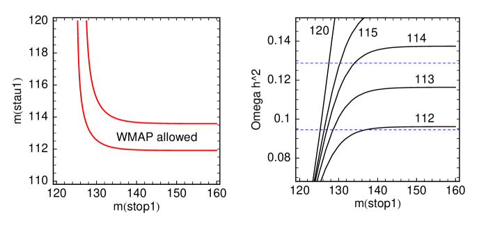
Figure 1: Neutralino relic density for $M_{1}=110$ GeV, $M_{2}=220$ GeV, $\mu=300$ GeV, $\tan\beta=7$: in a) the WMAP allowed band in $m_{\tilde{t}_{1}}$–$m_{\tilde{\tau}_{1}}$ plane, and in b) $\Omega h^{2}$ as a function of $m_{\tilde{t}_{1}}$ for various $\tilde{\tau}_{1}$ masses. Computed with micrOMEGAs 1.3. All masses are in [GeV]. The other parameters are as explained in the text.

As the first scenario we take the parameter point $M_{1}=110$ GeV, $M_{2}=220$ GeV, $\mu=300$ GeV and $\tan\beta=7$. This gives a spectrum of $m_{\tilde{\chi}^{0}_{1...4}}=\{105,191,306,340\}$ GeV and $m_{\tilde{\chi}^{\pm}_{1,2}}=\{189,340\}$ GeV. The $\tilde{\chi}^{0}_{1}$ is dominantly a bino with only 1% wino and 5% higgsino admixture. With slepton masses around 250 GeV, squark masses around 1 TeV and $m_{A}\gg 2m_{\tilde{\chi}^{0}_{1}}$, the $\tilde{\chi}^{0}_{1}$ annihilation cross section is much too low, leading to $\Omega h^{2}\sim 0.8$, which is well above the WMAP bound. One possibility to achieve the right $\Omega h^{2}$ is to lower $m_{A}$ to about 250 GeV. In this case the neutralinos annihilate efficiently through $\tilde{\chi}^{0}_{1}\tilde{\chi}^{0}_{1}\to A\to b\bar{b}$, leading to $\Omega h^{2}\sim 0.1$ (when closer to the pole of $m_{A}-2\tilde{\chi}^{0}_{1}$, the $\tilde{\chi}^{0}$’s annihilate too fast and $\Omega h^{2}$ becomes too small). Another possibility is to rely on co-annihilation with stops or staus. This puts rather strong constraints on the $\tilde{\tau}_{1}$ and/or $\tilde{t}_{1}$ masses, since stau co-annihilation occurs for $m_{\tilde{\tau}_{1}}-m_{\tilde{\chi}^{0}_{1}}\;\raisebox{-3.87495pt}{$\textstyle\stackrel{{\scriptstyle\textstyle<}}{{\sim}}$}\;10$ GeV while stop co-annihilation requires $m_{\tilde{t}_{1}}-m_{\tilde{\chi}^{0}_{1}}\;\raisebox{-3.87495pt}{$\textstyle\stackrel{{\scriptstyle\textstyle<}}{{\sim}}$}\;25$ GeV. These constraints imply that the decay products of the staus or stops will be difficult to detect at a hadron collider.

Figure 1a shows the WMAP-allowed band in the $m_{\tilde{t}_{1}}$–$m_{\tilde{\tau}_{1}}$ plane for $\tilde{t}_{1}\sim\tilde{t}_{\rm R}$ and $\tilde{\tau}_{1}\sim\tilde{\tau}_{\rm R}$, $m_{A}=1$ TeV and the other parameters as explained above. Figure 1b shows the neutralino relic density as a function of $m_{\tilde{t}_{1}}$ for various values of $m_{\tilde{\tau}_{1}}$. As can be seen, the WMAP bound puts a lower limit on the $\tilde{t}_{1}$ and $\tilde{\tau}_{1}$ masses of $m_{\tilde{t}_{1}}\;\raisebox{-3.87495pt}{$\textstyle\stackrel{{\scriptstyle\textstyle>}}{{\sim}}$}\;125$ GeV and $m_{\tilde{\tau}_{1}}\;\raisebox{-3.87495pt}{$\textstyle\stackrel{{\scriptstyle\textstyle>}}{{\sim}}$}\;112$ GeV (which is, however, only a stringent bound if one requires that the LSP provide all the cold dark matter). It can also put an upper limit on one mass as a function of the other. This bound is more severe. For example, for $m_{\tilde{t}_{1}}\;\raisebox{-3.87495pt}{$\textstyle\stackrel{{\scriptstyle\textstyle>}}{{\sim}}$}\;130$ GeV agreement with WMAP requires $m_{\tilde{\tau}_{1}}\;\raisebox{-3.87495pt}{$\textstyle\stackrel{{\scriptstyle\textstyle<}}{{\sim}}$}\;114$ GeV if no other process helps the $\tilde{\chi}^{0}_{1}$ annihilate efficiently. The exact masses of the other sleptons and squarks are not important for the computation of the relic density in this example because they are too heavy to contribute significantly in (co-)annihilation processes.

2.2 $M_{1}=110$ GeV, $\mu=180$ GeV, $\tan\beta=7$

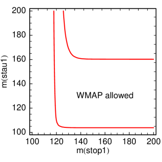
Figure 2: WMAP allowed band in the $m_{\tilde{t}_{1}}$–$m_{\tilde{\tau}_{1}}$ plane analogous to Fig. 1a, but for $\mu=180$ GeV.

For the second scenario, we lower $\mu$ to 180 GeV, keeping the other parameters as above. This leads to $m_{\tilde{\chi}^{0}_{1...4}}=\{93,152,188,274\}$ GeV and $m_{\tilde{\chi}^{\pm}_{1,2}}=\{139,273\}$ GeV. The $\tilde{\chi}^{0}_{1}$ has now 4% wino and 25% higgsino admixture and annihilates quite efficently into $W^{+}W^{-}$, giving a relic density of $\Omega h^{2}=0.138$. We hence need only a small additional contribution to $\langle\sigma v\rangle$, e.g. from light staus or stops, or from Higgs exchange.

Figure 2 shows the WMAP allowed band in the $m_{\tilde{t}_{1}}$–$m_{\tilde{\tau}_{1}}$ plane for this scenario. The allowed region is much larger than in Fig. 1a, especially because for $m_{\tilde{t}_{1}}\;\raisebox{-3.87495pt}{$\textstyle\stackrel{{\scriptstyle\textstyle>}}{{\sim}}$}\;130$ GeV, t-channel exchange of $\tilde{\tau}_{1}$ with $m_{\tilde{\tau}_{1}}\;\raisebox{-3.87495pt}{$\textstyle\stackrel{{\scriptstyle\textstyle<}}{{\sim}}$}\;160$ GeV is sufficient to bring $\Omega h^{2}$ into the desired range. For $m_{\tilde{\tau}_{1}}\;\raisebox{-3.87495pt}{$\textstyle\stackrel{{\scriptstyle\textstyle<}}{{\sim}}$}\;105$ GeV, on the other hand, stau co-annihilation comes into play, driving $\Omega h^{2}$ below the $2\sigma$ WMAP bound. Likewise, $\Omega h^{2}$ turns out too low for $m_{\tilde{t}_{1}}\;\raisebox{-3.87495pt}{$\textstyle\stackrel{{\scriptstyle\textstyle<}}{{\sim}}$}\;120$ GeV because of co-annihilation with stops. Note, however, that in this scenario a $\tilde{t}_{1}$ heavier than about 144 GeV will decay into $b\tilde{\chi}^{+}_{1}$ rather than into $c\tilde{\chi}^{0}_{1}$, which gives additional $b$ jets and, more importantly, additional same-sign leptons. This changes the signature of Eq. (2) to

$$\tilde{g}\tilde{g}\to bb\bar{b}\bar{b}\,l^{+}l^{+}l^{-}l^{-}+E_{T}^{\rm miss}\,,$$ (4)

or more generally to $4b+4W+E_{T}^{\rm miss}$. It is clear that the information from the same-sign top quarks is lost in this way.

3 Case study for the LHC

3.1 Choice of parameters

In order to explore the feasibility of extracting the light stop signal Eq. (2) at the LHC, we perform a case study for the parameters of Sect. 2.1 ($M_{1}=110$ GeV, $\mu=300$ GeV, $\tan\beta=7$), $m_{\tilde{t}_{1}}=150$ GeV and $m_{\tilde{g}}=660$ GeV, assuming BR$(\tilde{t}_{1}\to c\tilde{\chi}^{0}_{1})=1$. All squark mass parameters apart from $m_{\tilde{U}_{3}}$ are set to 1 TeV in order to maximise BR$(\tilde{g}\to t\tilde{t}_{1})$ and suppress background from e.g. $\tilde{b}\to t\tilde{\chi}^{-}$ decays. For the sleptons, we take $M_{\tilde{L},\tilde{E}}=250$ GeV. As explained in Sect. 2.1, agreement with WMAP can be achieved by $m_{A}\simeq 250$ GeV or, if $m_{A}$ is large, by $m_{\tilde{\tau}_{1}}\simeq 112$–113 GeV. In what follows we use $m_{A}=250$ GeV. We call this the LST1 scenario. The parameters and the resulting mass spectrum calculated with SuSpect 2.3 [21] are given in Tables 3 and 4, respectively. Note that the SUSY-breaking parameters in Table 3 are taken to be on-shell.

$M_{1}$	$M_{2}$	$M_{3}$	$\mu$	$\tan(\beta)$
110	220	660	300	7
$m_{A}$	$A_{t}$	$A_{b}$	$A_{\tau}$
250	$-670$	$-500$	100
$m_{\tilde{L}_{1,2}}$	$m_{\tilde{L}_{3}}$	$m_{\tilde{Q}_{1,2}}$	$m_{\tilde{Q}_{3}}$
250	250	1000	1000
$m_{\tilde{E}_{1,2}}$	$m_{\tilde{E}_{3}}$	$m_{\tilde{U}_{1,2}}$	$m_{\tilde{D}_{1,2}}$	$m_{\tilde{U}_{3}}$	$m_{\tilde{D}_{3}}$
250	250	1000	1000	100	1000
$\alpha_{\mathrm{e}m}^{-1}(m_{Z})^{\overline{\mathrm{MS}}}$	$G_{F}$	$\alpha_{s}(m_{Z})^{\overline{\mathrm{MS}}}$	$m_{Z}$	$m_{b}(m_{b})^{\overline{\mathrm{MS}}}$	$m_{t}$	$m_{\tau}$
127.91	$1.1664\times 10^{-5}$	0.11720	91.187	4.2300	175.0	1.7770

Table 3: Input parameters for the LST1 scenario [masses in GeV]. Unless stated otherwise, the SM masses are pole masses.

$\tilde{d}_{L}$	$\tilde{u}_{L}$	$\tilde{b}_{1}$	$\tilde{t}_{1}$	$\tilde{e}_{L}$	$\tilde{\tau}_{1}$	$\tilde{\nu}_{e}$	$\tilde{\nu}_{\tau}$
1001.69	998.60	997.43	149.63	254.35	247.00	241.90	241.90
$\tilde{d}_{R}$	$\tilde{u}_{R}$	$\tilde{b}_{2}$	$\tilde{t}_{2}$	$\tilde{e}_{R}$	$\tilde{\tau}_{2}$
1000.30	999.40	1004.56	1019.26	253.55	260.73
$\tilde{g}$	$\tilde{\chi}^{0}_{1}$	$\tilde{\chi}^{0}_{2}$	$\tilde{\chi}^{0}_{3}$	$\tilde{\chi}^{0}_{4}$	$\tilde{\chi}^{\pm}_{1}$	$\tilde{\chi}^{\pm}_{2}$
660.00	104.81	190.45	306.06	340.80	188.64	340.09
$h$	$H$	$A$	$H^{\pm}$
118.05	251.52	250.00	262.45

Table 4: SUSY mass spectrum [in GeV] for the LST1 scenario. For the squarks and sleptons, the first two generations have identical masses.

3.2 Monte Carlo simulation

We have generated SUSY events and $t\bar{t}$ background equivalent to $30~{}\text{fb}^{-1}$ of integrated luminosity with PYTHIA 6.321 [22] and CTEQ 5L parton distribution functions [23], corresponding to three years running of the LHC at low luminosity. The SUSY NLO cross sections are found in Table 5. We have also generated additional SM background in five logarithmic $p_{T}$ bins from $p_{T}=50$ GeV to $4000$ GeV, consisting of $5\times 10^{4}$ of $W+\rm jet$, $Z+\rm jet$, and $WW/WZ/ZZ$ production and $3.5\times 10^{5}$ QCD $2\rightarrow 2$ events per bin.

	$\sigma(\tilde{t}_{1}\tilde{t}_{1})$	$\sigma(\tilde{g}\tilde{g})$	$\sigma(\tilde{g}\tilde{q})$	$\sigma(\tilde{\chi}^{0}_{2}\tilde{\chi}^{\pm}_{1})$	$\sigma(\tilde{\chi}^{\pm}_{1}\tilde{\chi}^{\mp}_{1})$	$\sigma(\tilde{q}\tilde{q})$	$\sigma(\tilde{q}\tilde{q}^{*})$	$\sigma(\tilde{\chi}^{\pm}_{1}\tilde{g})$	$\sigma(t\bar{t})$
LST1	$280$	$5.39$	$4.98$	$1.48$	$0.774$	$0.666$	$0.281$	$0.0894$	$737$

Table 5: The main SUSY NLO cross sections in pb for the LST1 scenario, computed with Prospino2 [12]. For comparison, we also give the $t\bar{t}$ NLO cross section taken from [20].

Detector simulation has been done using the generic LHC detector simulation
AcerDET 1.0 [24]. This expresses identification and isolation of leptons and jets in terms of detector coordinates by azimuthal angle $\phi$, pseudo-rapidity $\eta$ and cone size $\Delta R=\sqrt{(\Delta\phi)^{2}+(\Delta\eta)^{2}}$. We identify a lepton if $p_{T}>5(6)$ GeV and $|\eta|<2.5$ for electrons (muons). A lepton is isolated if it is at a distance $\Delta R>0.4$ from other leptons and jets, and if the transverse energy deposited in a cone $\Delta R=0.2$ around the lepton is less than $10$ GeV. Jets are reconstructed by a cone-based algorithm from clusters and are accepted if the jet has $p_{T}>15$ GeV in a cone $\Delta R=0.4$. The jets are re-calibrated using a flavour independent parametrisation, optimised to give a proper scale for the dijet decay of a light (100–120 GeV) Higgs boson. The $b$-tagging efficiency and light jet rejection is set according to the $p_{T}$ parametrization for a low luminosity environment given in [25].

3.3 Effective mass

In Fig. 3 we show the distribution of the effective mass $M_{\text{eff}}$,

$$M_{\text{eff}}=E_{T}^{\rm miss}+\sum_{i}p^{\text{jet}}_{T,i},$$ (5)

for the LST1 scenario under study. The cuts used are:

• Require at least four jets with $p^{\text{jet}}_{T}>100,100,50,50$ GeV in each event.

• No isolated electrons or muons.

• $E_{T}^{\rm miss}>\max(100,0.25\sum p^{\text{jet}}_{T})$ GeV.

The clear excess of events toward high values of $M_{\text{eff}}$, compared to the SM distribution, indicates that SUSY should be easily discovered in our light stop scenario.

The effective mass has also been shown (see [26, 27]) to work as a measurement of the effective SUSY mass scale, $M^{\text{eff}}_{\text{susy}}$, given by

$$M^{\text{eff}}_{\text{susy}}=M_{\text{susy}}-\frac{m_{\tilde{\chi}^{0}_{1}}^{2}}{M_{\text{susy}}},$$ (6)

where the SUSY mass scale, $M_{\text{susy}}$, is a cross section weighted average of the masses of the initially produced SUSY particles; usually gluinos and squarks. In the light stop scenario, stop pair production overwhelmingly dominates the SUSY cross section. Yet it is difficult to extract the stop mass from the effective mass in this manner, since the cuts placed to handle the SM background also remove most of the stop pair production events. What remains is mostly gluino-pair production and gluino-squark production, and we can instead use the effective mass to estimate the gluino mass. In [27] the linear regression relationship $M_{\text{est}}=1.7M^{\text{eff}}_{\text{susy}}+134.15$ GeV, where $M_{\text{est}}$ is the fitted peak of the $M_{\text{eff}}$ distribution, was found from a large set of random mSUGRA and MSSM models. The joint statistical and systematic error on the SUSY mass scale from using this relationship was estimated to be below 40% after one year running of the LHC at low luminosity. With the peak effective mass value of $M_{\text{est}}\simeq 1023$ GeV at LST1, and a conservative estimate of accuracy at the level of 30% after $30~{}\text{fb}^{-1}$ of integrated luminosity, this gives $M^{\text{eff}}_{\text{susy}}=523\pm 157$ GeV. This may serve as a first estimate of the gluino mass scale.

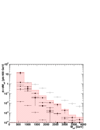
Figure 3: Effective mass distribution. SM contributions are $t\bar{t}$ (filled circles), $W$+jet (triangles), $Z$+jet (inverted triangles), $WW/WZ/ZZ$ production (stars) and QCD (squares). The sum of all SM events is shown by the hatched histogram. SUSY events are shown as open circles.

3.4 Signal isolation

The peculiar nature of the signal with a same-sign top pair will serve to remove most of the background, both SM and SUSY. We use the following cuts:

• Require two same sign leptons ($e$ or $\mu$) with $p^{\text{lep}}_{T}>20$ GeV.

• Require at least four jets with $p^{\text{jet}}_{T}>50$ GeV, at least two of which are $b$-tagged.

• $E_{T}^{\rm miss}>100$ GeV.

• We cut on top content in the events by requiring two combinations of leptons and $b$-jets to give invariant masses $m_{bl}<160$ GeV, consistent with a top.

The effects of these cuts are shown in Table 6. The column “2lep 4jet” gives the status after detector simulation and cuts on two reconstructed and isolated leptons and four reconstructed jets; “2$b$” is the number of events left after the $b$-jet cut, assuming a $b$-tagging efficiency of $43\%$; “$E_{T}^{\rm miss}$” is the cut on missing transverse energy and “SS” the requirement of two same-sign leptons. These cuts constitute the signature of Eq. (2). Note the central importance of the same-sign cut in removing the SM background, which at that point consists only of $t\bar{t}$ events. The cuts on transverse momentum and top content “2$t$” are used to further reduce the background. We find that the gluino-pair production, followed by gluino decay into top and stop and leptonic top decay, is easily separated from the background.

Cut	2lep 4jet	$p_{T}^{\text{lep}}$	$p_{T}^{\text{jet}}$	2$b$	$E_{T}^{\rm miss}$	2$t$	SS
Signal
$\tilde{g}\tilde{g}$	10839	6317	4158	960	806	628	330
Background
SUSY	1406	778	236	40	33	16	5
SM	25.3M	1.3M	35977	4809	1787	1653	12

Table 6: Number of events left after cumulative cuts for $30~{}\text{fb}^{-1}$ of integrated luminosity.

To investigate other possible backgrounds to our signal we have used MadGraph II with the MadEvent event generator [28, 29]. The search has been limited to parton level, as we find no processes that can contribute after placing appropriate cuts. We have looked at SM processes that can mimic a same-sign top pair by mis-tagging of jets or the production of one or more additional leptons, as well as inclusive production of same-sign top pairs. We assume that the two extra jets needed in some cases could be produced by ISR, FSR, or the underlying event. In particular we have looked at diffractive scattering $qq\to W^{\pm}q^{\prime}W^{\pm}q^{\prime}$ and the production of a top pair from gluon radiation in single $W$ production $qq^{\prime}\to t\bar{t}W^{\pm}$. Also checked is the production of $t\bar{t}l^{+}l^{-}$, $t\bar{t}t\bar{t}$, $t\bar{t}t\bar{b}$, $t\bar{t}b\bar{t}$, $tW^{-}tW^{-}$, $\bar{t}W^{+}\bar{t}W^{+}$ and $W^{\pm}W^{\pm}b\bar{b}jj$. We place cuts on leptons and quarks as given above, and demand two lepton-quark pairs consistent with top decays. We also require neutrinos from the $W$ decays to give the required missing energy. After these cuts and reasonable detector geometry cuts of $\Delta R>0.4$ and $|\eta|<2.5$ for all leptons and quarks, we find that the cross-sections of all of these processes are too small, by at least an order of magnitude, to make a contribution at the integrated luminosity considered.

Last but not least we have assumed that there is no additional same-sign top production from flavour-changing neutral currents (FCNC), i.e. that the anomalous couplings in tgc(u) vertices are effectively zero. See [30] for a discussion on same-sign tops in FCNC scenarios.

3.5 Determining masses

Having isolated the decay chain it will be important to measure the properties of the sparticles involved to confirm that the decay indeed involves a light scalar top. Since the neutralino and the neutrino in the top decay represent missing momentum and energy, reconstruction of a mass peak is impossible. The well studied alternative to this, see e.g. [26, 31, 32, 33, 34], is to use the invariant-mass distributions of the SM decay products. Their endpoints can be given in terms of the SUSY masses involved, and these equations can then in principle be solved to give the masses.

In our scenario there are two main difficulties with this. First, there are four possible endpoints: $m_{bl}^{\max}$, $m_{bc}^{\max}$, $m_{lc}^{\max}$ and $m_{blc}^{\max}$, of which the first simply gives a relationship between the masses of the $W$ and the top, and the second and third are linearly dependent, so that we are left with three unknown masses and only two equations. Second, because of the information lost with the escaping neutrino the distributions of interest all fall very gradually to zero. Determining exact endpoints in the presence of background, while taking into account smearing from the detector, effects of particle widths etc. will be very difficult. The shapes of the invariant-mass distributions are shown, for some arbitrary normalization, in Fig. 4.

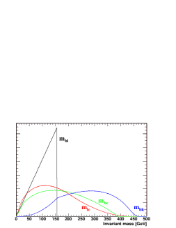
Figure 4: Invariant-mass distributions for LST1. These distributions only take into account the kinematics of the decay, i.e. no spin or width effects are included.

In what follows we have partially solved the second problem by extending the endpoint method and deriving analytic expressions for the shape of the invariant-mass distributions $m_{bc}$ and $m_{lc}$. The derivation is given in Appendix A. These shapes can now be used to fit the whole distributions of the isolated signal events and not just the endpoints. This greatly reduces the uncertainty involved in endpoint determination, and provides the possibility of getting more information on the masses. One could also imagine extending this method to include spin effects in the distribution, to get a handle on the spins of the SUSY particles involved and possibly confirming the scalar nature of the stop.

In fitting the $m_{bc}$ and $m_{lc}$ distributions, we start from the isolated $\tilde{g}\tilde{g}$ signal of Section 3.4. However, these events contain some where one or both of the $W$ decay to a tau, which in turn decays leptonically. These taus are an additional, irreducible background to our distributions. The $b$-jets and leptons are paired through the cut on two $t$ quark candidates. A comparison with Monte Carlo truth information from the event generation shows that this works well in picking the right pairs. The issue which remains is to identify the $c$-quark initiated jets and to assign these to the correct $b$-jet and lepton pair. The precision of our mass determination is limited by systematics from these problems.

Two different strategies can be used for picking the $c$-jets. The strong correlation between the tagging of $b$- and $c$-jets suggest an inclusive $b/c$-jet tagging of at least four jets per event. The two types of jets can then be separated on their $b$-tagging likelihoods, and the requirement of two top candidates in the event. A thorough investigation of this strategy requires a full simulation study, using realistic $b$-tagging routines. The other strategy, which we follow here, is to accept a low $b$-tagging efficiency to pick two $b$-jets and reject most $c$-jets. The likelihoods in the $b$-tagging routine can then help pick the correct $c$-jets from the remaining jets. In this fast simulation study we are restricted to a simple statistical model of the efficiency of making this identification. We have looked at two cases: One worst case scenario with no direct $c$-jet identification, where we only use the kinematics of the event to pick out the $c$-jets, and one where we have assumed an additional $20\%$ probability of identifying a $c$-jet directly from the $b$-tagging likelihood.

For events where we have missed one or both $c$-jets, they are picked as the two hardest remaining jets with $p_{T}^{\text{jet}}<100$ GeV. The upper bound on transverse momentum is applied because the stop is expected to be relatively light if our signal exists, and it avoids picking jets from the decay of heavy squarks. Our $c$-jet candidates are paired to the top candidates by their angular separation in the lab frame, and by requiring consistency with the endpoints of the two invariant-mass distributions we are not looking at. E.g. if we wish to construct the $m_{bc}$ distribution we demand consistency with the endpoints $m_{lc}^{\max}$ and $m_{blc}^{\max}$ . Events with no consistent combinations of $c$-jets and top candidates are rejected.

The fit functions for $m_{bc}$ and $m_{lc}$ are given in Eqs. (24) and (48). In principle both of the two linearly independent parameters $m_{bc}^{\max}$ and $a$ could be determined by fits. However, we typically have $m_{t}m_{\tilde{t}_{1}}\ll m_{\tilde{g}}^{2}$ for light stops, so that $a\approx 1$. For LST1, the nominal value is $a=0.991$. The distributions are sensitive to such values of $a$ only at very low invariant masses. Because of the low number of events, no sensible value can be determined from a fit; we therefore set $a=1$. The fit quality and value of $m_{bc}^{\max}$ is found to be insensitive to the choice of $a$ for $a\;\raisebox{-3.87495pt}{$\textstyle\stackrel{{\scriptstyle\textstyle>}}{{\sim}}$}\;0.980$.

The results of the fits to $m_{bc}^{\max}$, assuming no $c$-jet tagging, are shown in Fig. 5. The combined result of the two distributions is $m_{bc}^{\max}=383.2\pm 4.9$ GeV, to be compared with the nominal value of $391.1$ GeV. The large $\chi^{2}$ values of the fits and the low value of $m_{bc}^{\max}$ indicate that there are some significant systematical errors. Comparing to Monte Carlo truth information we have found that the peaks at around $100-150$ GeV, responsible for the bad fit quality, are chiefly the result of events with one or more taus (see above). In Fig. 6 we show the results assuming $20\%$ $c$-tagging efficiency. The combined result has improved to $m_{bc}^{\max}=389.8\pm 5.3$ GeV. We expect to be able to do better than this with full information from the $b$-tagging routine.

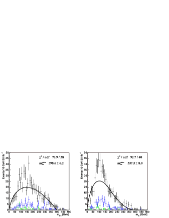
Figure 5: Invariant-mass distributions without $c$-jet tagging (black with error bars) and best fit. Left panel shows $m_{bc}$, right panel $m_{lc}$. Also shown are the contributions from the SM background (green) and the SUSY background (blue). The SUSY background consists mostly of events with one or more taus (see text).

Figure 6: Invariant-mass distributions with $20\%$ $c$-tagging efficiency after $b$-tagging. For details see caption of Figure 5.

4 Conclusions

We have investigated a baryogenesis-motivated scenario of a light stop ($m_{\tilde{t}_{1}}\;\raisebox{-3.87495pt}{$\textstyle\stackrel{{\scriptstyle\textstyle<}}{{\sim}}$}\;m_{t}$), with $\tilde{t}_{1}\to c\tilde{\chi}^{0}_{1}$ as the dominant decay mode. In this scenario, pair production of $\tilde{t}_{1}$ leads to a signature of two jets and missing transverse energy, which is all but promising for the discovery of $\tilde{t}_{1}$ at the LHC.

We have hence proposed a method which uses instead stops stemming from gluino decays: in gluino pair production, the Majorana nature of the gluino leads to a peculiar signature of same-sign top quarks in half of the gluino-to-stop decays. For the case that all other squarks are heavier than the gluino, we have shown that the resulting signature of $2b$’s + 2 same-sign leptons + jets $+E_{T}^{\rm miss}$ can be extracted from the background and serve as a discovery channel for a light $\tilde{t}_{1}$.

We have also demonstrated the measurement of a relationship between the gluino, stop and LSP masses. Taken together with a determination of other invariant-mass endpoints, and a measurement of the SUSY mass scale from the effective mass scale of events, this may be sufficient to determine the masses of the SUSY particles involved. In particular, if the invariant-mass distributions of the isolated events fit the predicted shapes, this strengthens the interpretation of the events as gluino decays into a top and a stop.

Last but not least some comments are in order on the robustness of the signal. While our analysis has been done for $m_{\tilde{g}}=660$ GeV, we have checked that the signal remains significant enough for a 5$\sigma$ discovery for gluino masses up to $m_{\tilde{g}}\sim$ 900 GeV. In the high-mass region, gluino-squark production with subsequent squark decay to gluino is responsible for a significant fraction of events. On the other hand, if sbottoms are lighter than assumed for LST1, they will contribute to the SUSY background through $\tilde{b}_{i}\to t\tilde{\chi}^{\pm}_{j}$ ($i,j=1,2$) decays. For instance, lowering the sbottom masses by a factor of 2, while keeping all other parameters as in LST1, would increase the background after cuts by 5 events. While this is not dramatic, the fits to invariant-mass distributions are worse because of the opening up of new gluino decays $\tilde{g}\to b\tilde{b}_{i}$. Lowering the stop mass while keeping the LSP mass fixed, entering the stop-coannihilation region, should also make the signal more difficult to find because the $c$-jets become too soft. Still, we find only a 12% decrease in the signal when setting $m_{\tilde{t}_{1}}=120$ GeV. This can be explained by a large number of signal events passing the cuts because of squark decays to gluinos producing an extra jet. This implies that the same-sign tops can be used to search for a light stop even in the stop-coannihilation channel, unreachable at the Tevatron. The fit to the invariant-mass shapes is again worse than for LST1.

We conclude that if $\tilde{t}_{1}$ decays into $c\tilde{\chi}^{0}_{1}$, light stops may be discovered through the search for same-sign tops in the decay of pairs of gluinos for a wide range of SUSY masses. A relation between the gluino, stop and LSP masses can be determined from invariant-mass distributions. In this paper we have demonstrated the feasibility of our method; a full simulation will clearly be necessary to assess its full potential.

Appendix A Derivation of shape formulae

The differential decay width for two independent angular variables (cosines) $u$ and $v$, in a decay with a given spin configuration, is

$$\frac{1}{\Gamma}\frac{\partial^{2}\Gamma}{\partial u\partial v}=f_{u}(u)\theta(u-1)\theta(1-u)f_{v}(v)\theta(v-1)\theta(1-v),$$ (7)

where the spin information is contained in the functions $f_{u}(u)$ and $f_{v}(v)$ and the theta functions are ordinary step function, limiting the values of $u$ and $v$ that give non-zero decay width.

By a change of variables one can easily go from an expression of the invariant-mass in terms of these variables, to the distribution sought. Given the invariant-mass $m(u,v)$, we have

$$\frac{1}{\Gamma}\frac{\partial\Gamma}{\partial m^{2}} = \int_{-\infty}^{\infty}\frac{1}{\Gamma}\frac{\partial^{2}\Gamma}{\partial m^{2}\partial v}dv$$ (8)

$$= \int_{-\infty}^{\infty}\left|\frac{\partial\left(u,v\right)}{\partial\left(m^{2},v\right)}\right|\frac{1}{\Gamma}\frac{\partial^{2}\Gamma}{\partial u\partial v}dv.$$

An extension to three or more independent angular variables is trivial.

We now proceed to derive the shape of the distribution of the invariant-masse of the $b$- and the $c$-quark, $m_{bc}$, and the invariant-mass of the lepton and the $c$-quark, $m_{lc}$. We will assume that all particles are spin-0, so that we have isotropic decays in particle rest frames. This lets us set $f_{u}$ and $f_{v}$ to be constant. This result is what we expect when summing over all final states. Effects of non-zero spin can be introduced via these functions. We also assume that the lighter quarks, $b$ and $c$, are massless.

A.1 $m_{bc}$

In the rest frame (RF) of the stop, energy and momentum conservation in the decay of the gluino, stop and top gives

$$E_{c}^{\tilde{t}_{1}} = \frac{m_{\tilde{t}_{1}}^{2}-m_{\tilde{\chi}_{1}^{0}}^{2}}{2m_{\tilde{t}_{1}}},$$ (9)

$$E_{t}^{\tilde{t}_{1}} = \frac{m_{\tilde{g}}^{2}-m_{t}^{2}-m_{\tilde{t}_{1}}^{2}}{2m_{\tilde{t}_{1}}},$$ (10)

$$E_{b}^{\tilde{t}_{1}} = \frac{m_{t}^{2}-m_{W}^{2}}{2E_{t}^{\tilde{t}_{1}}-2\sqrt{(E_{t}^{\tilde{t}_{1}})^{2}-m_{t}^{2}}\cos\theta_{tb}^{\tilde{t}_{1}}},$$ (11)

where $E_{c}^{\tilde{t}_{1}}$, $E_{t}^{\tilde{t}_{1}}$ and $E_{b}^{\tilde{t}_{1}}$ are the energies of $c$, $t$ and $b$ respectively in the stop RF and $\theta_{tb}^{\tilde{t}_{1}}$ is the angle between $t$ and $b$ in that frame.

We can rewrite $\cos\theta_{tb}^{\tilde{t}_{1}}$ in terms of an isotropically distributed angle, $\theta_{\tilde{g}b}^{t}$, in the top RF. By expressing $m_{\tilde{g}b}^{2}$ in the two rest frames, and since $\cos\theta_{tb}^{\tilde{t}_{1}}=\cos\theta_{\tilde{g}b}^{\tilde{t}_{1}}$, we get

$$E_{b}^{\tilde{t}_{1}}(E_{\tilde{g}}^{\tilde{t}_{1}}-\sqrt{(E_{\tilde{g}}^{\tilde{t}_{1}})^{2}-m_{\tilde{g}}^{2}}\cos\theta_{tb}^{\tilde{t}_{1}})=E_{b}^{t}(E_{\tilde{g}}^{t}-\sqrt{(E_{\tilde{g}}^{t})^{2}-m_{\tilde{g}}^{2}}\cos\theta_{\tilde{g}b}^{t}).$$ (12)

In the top RF, from the conservation of energy and momentum in the decays of the gluino and the top, we have that:

$$E_{b}^{t} = \frac{m_{t}^{2}-m_{W}^{2}}{2m_{t}},$$ (13)

$$E_{\tilde{g}}^{t} = \frac{m_{\tilde{g}}^{2}+m_{t}^{2}-m_{\tilde{t}_{1}}^{2}}{2m_{t}}.$$ (14)

Solving for $\cos\theta_{tb}^{\tilde{t}_{1}}$, using (10), (11), (13) and (14), we then arrive at

$$\cos\theta_{tb}^{\tilde{t}_{1}}=\frac{a-\cos\theta_{\tilde{g}b}^{t}}{1-a\cos\theta_{\tilde{g}b}^{t}}$$ (15)

where $a$ is given by

$$a=\frac{m_{2}^{2}}{m_{1}^{2}},$$ (16)

with $m_{1}$ and $m_{2}$ defined as

$$m_{1}^{2} = m_{\widetilde{g}}^{2}-m_{t}^{2}-m_{\widetilde{t}_{1}}^{2},$$ (17)

$$m_{2}^{4} = m_{1}^{4}-4m_{t}^{2}m_{\widetilde{t}_{1}}^{2}.$$ (18)

We can now find an expression for $m_{bc}^{2}:$

$$m_{bc}^{2} = 2E_{b}^{\tilde{t}_{1}}E_{c}^{\tilde{t}_{1}}\left(1-\cos\theta_{bc}^{\tilde{t}_{1}}\right)$$ (19)

$$= \left(m_{bc}^{\max}\right)^{2}\left(\frac{1-a\cos\theta_{\tilde{g}b}^{t}}{1+a}\right)\left(\frac{1-\cos\theta_{bc}^{\tilde{t}_{1}}}{2}\right),$$

where the endpoint of the distribution, $m_{bc}^{\max}$, is

$$\left(m_{bc}^{\max}\right)^{2}=\frac{\left(m_{t}^{2}-m_{W}^{2}\right)}{m_{t}^{2}}\frac{\left(m_{\widetilde{t}_{1}}^{2}-m_{\widetilde{\chi}_{1}^{0}}^{2}\right)\left(m_{1}^{2}+m_{2}^{2}\right)}{2m_{\widetilde{t}_{1}}^{2}}.$$ (20)

Using the switch of variables

$$u=\frac{1-\cos\theta_{bc}^{\tilde{t}_{1}}}{2},\quad\quad v=\frac{1-\cos\theta_{\tilde{g}b}^{t}}{2},$$ (21)

we can write the invariant-mass as

$$m_{bc}^{2}=\left(m_{bc}^{\max}\right)^{2}\left(\frac{1-a+2av}{1+a}\right)u.$$ (22)

From Eq. (8), and setting $f_{u}(u)=f_{v}(v)=1$, we find the distribution of the invariant-mass

$$\frac{1}{\Gamma}\frac{\partial\Gamma}{\partial m_{bc}^{2}} = \int_{-\infty}^{\infty}\left|\frac{\partial\left(u,v\right)}{\partial\left(m_{bc}^{2},v\right)}\right|\theta\left(u\right)\theta\left(1-u\right)\theta\left(v\right)\theta\left(1-v\right)dv$$ (23)

$$= \frac{1+a}{\left(m_{bc}^{\max}\right)^{2}}\int_{0}^{1}\frac{1}{1-a+2av}\,\theta\left(1-\frac{m_{bc}^{2}\left(1+a\right)}{\left(m_{bc}^{\max}\right)^{2}\left(1-a+2av\right)}\right)dv.$$

The theta function leads to two different lower limits on the integration, depending on the value of $m_{bc}$. Performing the integration gives

$$\frac{1}{\Gamma}\frac{\partial\Gamma}{\partial m_{bc}^{2}}=\left\{\begin{array}[]{cl}\displaystyle\frac{1+a}{2a(m_{bc}^{\max})^{2}}\ln\frac{1+a}{1-a}&\text{for~{}~{}}0<m_{bc}^{2}<(m_{bc}^{\max})^{2}\frac{1-a}{1+a},\\ \displaystyle\frac{1+a}{2a\left(m_{bc}^{\max}\right)^{2}}\ln\frac{(m_{bc}^{\max})^{2}}{m_{bc}^{2}}&\text{for~{}~{}}\left(m_{bc}^{\max}\right)^{2}\frac{1-a}{1+a}<m_{bc}^{2}<(m_{bc}^{\max})^{2},\end{array}\right.$$ (24)

expressing the distribution in terms of two parameters, $a$ and $m_{bc}^{\max}$.

A.2 $m_{lc}$

In the top RF, energy and momentum conservation in the decay of the gluino, stop, top and $W$ gives, in addition to Eq. (13),

$$E_{l}^{t} = \frac{m_{t}m_{W}^{2}}{(m_{t}^{2}+m_{W}^{2})-(m_{t}^{2}-m_{W}^{2})\cos\theta_{Wl}^{t}},$$ (25)

$$E_{c}^{t} = \frac{m_{t}(m_{\tilde{t}_{1}}^{2}-m_{\tilde{\chi}_{1}^{0}}^{2})}{m_{1}^{2}-m_{2}^{2}\cos\theta_{\tilde{t}_{1}c}^{t}},$$ (26)

where $E_{l}^{t}$ and $E_{c}^{t}$ are the energies of $b$, $l$ and $c$ respectively in the top RF, $\theta_{Wl}^{t}$ is the angle between $W$ and $l$ in that frame and $\theta_{\tilde{t}_{1}c}^{t}$ is the angle between $\tilde{t}_{1}$ and $c$.

We again change angles to isotropically distributed angles (under spin-0 assumptions). From $\cos\theta_{Wl}^{t}=-\cos\theta_{bl}^{t}$, and expressing $m_{bl}^{2}$ in both the top and $W$ rest frames, we have

$$E_{b}^{t}E_{l}^{t}(1+\cos\theta_{Wl}^{t})=E_{b}^{W}E_{l}^{W}(1-\cos\theta_{bl}^{W}).$$ (27)

In the $W$ RF, energy and momentum conservation in the top and $W$ decays gives

$$E_{b}^{W} = \frac{m_{t}^{2}-m_{W}^{2}}{2m_{W}},$$ (28)

$$E_{l}^{W} = \frac{1}{2}m_{W}.$$ (29)

Using (13), (26), (28) and (29) we find that

$$\cos\theta_{Wl}^{t}=\frac{(m_{t}^{2}-m_{W}^{2})-(m_{t}^{2}+m_{W}^{2})\cos\theta_{bl}^{W}}{(m_{t}^{2}+m_{W}^{2})-(m_{t}^{2}-m_{W}^{2})\cos\theta_{bl}^{W}}.$$ (30)

From $\cos\theta_{\tilde{t}_{1}c}^{t}=\cos\theta_{\tilde{g}c}^{t}$, and expressing $m_{\tilde{g}c}^{2}$ in both the $t$ and $\tilde{t}_{1}$ rest frames we get

$$E_{c}^{t}(E_{\tilde{g}}^{t}-\sqrt{(E_{\tilde{g}}^{t})^{2}-m_{\tilde{g}}^{2}}\cos\theta_{\tilde{t}_{1}c}^{t})=E_{c}^{\tilde{t}_{1}}(E_{\tilde{g}}^{\tilde{t}_{1}}-\sqrt{(E_{\tilde{g}}^{\tilde{t}_{1}})^{2}-m_{\tilde{g}}^{2}}\cos\theta_{\tilde{g}c}^{\tilde{t}_{1}})$$ (31)

from which, using (9), (10), (14) and (26), it follows that

$$\cos\theta_{\tilde{t}_{1}c}^{t}=\frac{a-\cos\theta_{\tilde{g}c}^{\tilde{t}_{1}}}{1-a\cos\theta_{\tilde{g}c}^{\tilde{t}_{1}}}.$$ (32)

This could also have been found from (15), using a symmetry argument.

We can now find an expression for $m_{lc}^{2}:$

$$m_{lc}^{2} = 2E_{l}^{t}E_{c}^{t}\left(1-\cos\theta_{lc}^{t}\right)$$ (33)

$$= (m_{lc}^{\max})^{2}\left(\frac{1-a\cos\theta_{\tilde{g}c}^{\tilde{t}_{1}}}{1+a}\right)\left(\frac{m_{t}^{2}+m_{W}^{2}-\left(m_{t}^{2}-m_{W}^{2}\right)\cos\theta_{bl}^{W}}{2m_{t}^{2}}\right)\left(\frac{1-\cos\theta_{lc}^{t}}{2}\right),$$

where

$$(m_{lc}^{\max})^{2}=\frac{\left(m_{\tilde{t}_{1}}^{2}-m_{\tilde{\chi}_{1}^{0}}^{2}\right)\left(m_{1}^{2}+m_{2}^{2}\right)}{2m_{\tilde{t}_{1}}^{2}}.$$ (34)

Using the switch of variables

$$u=\frac{1-\cos\theta_{\tilde{g}c}^{\tilde{t}_{1}}}{2},\quad\quad v=\frac{1-\cos\theta_{bl}^{W}}{2},\quad\quad w=\frac{1-\cos\theta_{lc}^{t}}{2},$$ (35)

we can write

$$m_{lc}^{2}=(m_{lc}^{\max})^{2}\left(\frac{1-a+2au}{1+a}\right)\left(\frac{m_{W}^{2}+\left(m_{t}^{2}-m_{W}^{2}\right)v}{m_{t}^{2}}\right)w.$$ (36)

Since

$$\frac{1}{\Gamma}\frac{\partial^{3}\Gamma}{\partial u\partial v\partial m_{lc}^{2}} = \frac{1}{\Gamma}\frac{\partial^{3}\Gamma}{\partial u\partial v\partial w}\left|\frac{\partial\left(u,v,w\right)}{\partial\left(u,v,m_{lc}^{2}\right)}\right|$$ (37)

$$= \frac{m_{t}^{2}(1+a)\hat{\theta}(u)\hat{\theta}(v)\hat{\theta}(w)}{(m_{lc}^{\max})^{2}\left(1-a+2au\right)\left(m_{W}^{2}+\left(m_{t}^{2}-m_{W}^{2}\right)v\right)},$$

where $\hat{\theta}(x)=\theta(x)\theta(1-x)$, we have from a generalization of (8) that

$$\frac{1}{\Gamma}\frac{\partial\Gamma}{m_{lc}^{2}}=\frac{m_{t}^{2}(1+a)}{(m_{lc}^{\max})^{2}}\int_{0}^{1}\int_{0}^{1}\frac{\hat{\theta}(w)}{(1-a+2au)(m_{W}^{2}+(m_{t}^{2}-m_{W}^{2})v)}dudv.$$ (38)

The step functions for $w$ give more complicated bounds on the integration than what was the case for $m_{bc}$. We must have $m_{lc}^{2}>0$ and

$$m_{W}^{2}+(m_{t}^{2}-m_{W}^{2})v>\frac{m_{t}^{2}(1+a)m_{lc}^{2}}{(m_{lc}^{\max})^{2}(1-a+2au)}.$$ (39)

This integration and the integration limits from the last inequality are best explored by yet another change of variables

$$x=1-a+2au,\quad y=m_{W}^{2}+(m_{t}^{2}-m_{W}^{2})v,$$ (40)

from which the integral can be written

$$\frac{1}{\Gamma}\frac{\partial\Gamma}{m_{lc}^{2}}=\frac{1+a}{2a(m_{bc}^{\max})^{2}}\int_{m_{W}^{2}}^{m_{t}^{2}}\int_{1-a}^{1+a}\hat{\theta}\left(\frac{m_{lc}^{2}}{\left(m_{lc}^{\max}\right)^{2}}\frac{m_{t}^{2}(1+a)}{xy}\right)\frac{1}{xy}\,dxdy.$$ (41)

We note that there is a maximum of $m_{lc}^{2}<(m_{lc}^{\max})^{2}$, as expected. There are then five different possible shapes for the areas of integration in the $xy-$plane. For ease of notation we use

$$x_{1}=1-a,\quad x_{2}=1+a,\quad y_{1}=m_{W}^{2},\quad y_{2}=m_{t}^{2}.$$ (42)

The shapes can be categorized by bounds on $y(x_{1})$ and $y(x_{2})$ as found in Table 7.

Shape	$y(x_{1})$	$y(x_{2})$
I	$y_{2}<y(x_{1})$	$y_{1}<y(x_{2})<y_{2}$
II	$y_{1}<y(x_{1})<y_{2}$	$y_{1}<y(x_{2})<y_{2}$
III	$y_{2}<y(x_{1})$	$y(x_{2})<y_{1}$
IV	$y_{1}<y(x_{1})<y_{2}$	$y(x_{2})<y_{1}$
V	$y(x_{1})<y_{1}$	$y(x_{2})<y_{1}$

Table 7: Shapes for the area of integration for the integral in Eq. (41).

The inequalities in the categorization of the shapes can be expressed as bounds on $m_{lc}^{2}$:

$$y_{1} < y(x_{1})\Leftrightarrow(m_{lc}^{\max})^{2}\frac{(1-a)}{(1+a)}\frac{m_{W}^{2}}{m_{t}^{2}}<m_{lc}^{2},$$ (43)

$$y_{1} < y(x_{2})\Leftrightarrow(m_{lc}^{\max})^{2}\frac{m_{W}^{2}}{m_{t}^{2}}<m_{lc}^{2},$$ (44)

$$y_{2} < y(x_{1})\Leftrightarrow(m_{lc}^{\max})^{2}\frac{(1-a)}{(1+a)}<m_{lc}^{2},$$ (45)

$$y_{2} < y(x_{2})\Leftrightarrow(m_{lc}^{\max})^{2}<m_{lc}^{2}.$$ (46)

We can see that there will be two cases, depending on the mass hierarchy:

Case A: $$\frac{m_{W}^{2}}{m_{t}^{2}}<\frac{1-a}{1+a}$$

Case B:

(47)

We give the invariant-mass distribution for both of these cases.

Case A

Here Shape III is excluded, so the invariant-mass distribution is

$$\frac{1}{\Gamma}\frac{\partial\Gamma}{m_{lc}^{2}}=\left\{\begin{array}[]{lcl}\displaystyle\frac{1+a}{2a(m_{bc}^{\max})^{2}}\ln\frac{1+a}{1-a}\ln\frac{m_{t}^{2}}{m_{W}^{2}}&\text{for~{}}&0<m_{lc}^{2}<(m_{lc}^{\max})^{2}\frac{1-a}{1+a}\frac{m_{W}^{2}}{m_{t}^{2}},\\[14.22636pt] \lx@intercol\@ADDCLASS{ltx_eqn_lefteqn}$\displaystyle\frac{1+a}{2a(m_{bc}^{\max})^{2}}\left[\ln\frac{1+a}{1-a}\ln\frac{m_{t}^{2}}{m_{W}^{2}}-\frac{1}{2}\left(\ln\frac{1+a}{1-a}\frac{m_{t}^{2}}{m_{W}^{2}}\frac{m_{lc}^{2}}{(m_{lc}^{\max})^{2}}\right)^{2}\right]$\mbox{}\hfil\lx@intercol\hskip 85.35826pt\\[14.22636pt] &\text{for~{}}&(m_{lc}^{\max})^{2}\frac{1-a}{1+a}\frac{m_{W}^{2}}{m_{t}^{2}}<m_{lc}^{2}<(m_{lc}^{\max})^{2}\frac{m_{W}^{2}}{m_{t}^{2}},\\[14.22636pt] \lx@intercol\@ADDCLASS{ltx_eqn_lefteqn}$\displaystyle\frac{1+a}{2a(m_{bc}^{\max})^{2}}\ln\frac{1+a}{1-a}\left(\ln\frac{\left(m_{lc}^{\max}\right)^{2}}{m_{lc}^{2}}-\frac{1}{2}\ln\frac{1+a}{1-a}\right)$\mbox{}\hfil\lx@intercol\\[14.22636pt] &\text{for~{}}&(m_{lc}^{\max})^{2}\frac{m_{W}^{2}}{m_{t}^{2}}<m_{lc}^{2}<(m_{lc}^{\max})^{2}\frac{1-a}{1+a},\\[14.22636pt] \lx@intercol\@ADDCLASS{ltx_eqn_lefteqn}$\displaystyle\frac{1+a}{2a(m_{bc}^{\max})^{2}}\ln\frac{\left(m_{lc}^{\max}\right)^{2}}{m_{lc}^{2}}\left(\ln\frac{\left(m_{lc}^{\max}\right)^{2}}{m_{lc}^{2}}-\ln\left(2m_{t}^{2}\right)\right)$\mbox{}\hfil\lx@intercol\\[14.22636pt] &\text{for~{}}&(m_{lc}^{\max})^{2}\frac{1-a}{1+a}<m_{lc}^{2}<(m_{lc}^{\max})^{2}.\end{array}\right.$$ (48)

Case B

Here Shape II is excluded, giving

$$\frac{1}{\Gamma}\frac{\partial\Gamma}{m_{lc}^{2}}=\left\{\begin{array}[]{lcl}\displaystyle\frac{1+a}{2a(m_{bc}^{\max})^{2}}\ln\frac{1+a}{1-a}\ln\frac{m_{t}^{2}}{m_{W}^{2}}&\text{for~{}}&0<m_{lc}^{2}<(m_{lc}^{\max})^{2}\frac{1-a}{1+a}\frac{m_{W}^{2}}{m_{t}^{2}},\\[14.22636pt] \lx@intercol\@ADDCLASS{ltx_eqn_lefteqn}$\displaystyle\frac{1+a}{2a(m_{bc}^{\max})^{2}}\left[\ln\frac{1+a}{1-a}\ln\frac{m_{t}^{2}}{m_{W}^{2}}-\frac{1}{2}\left(\ln\frac{1+a}{1-a}\frac{m_{t}^{2}}{m_{W}^{2}}\frac{m_{lc}^{2}}{(m_{lc}^{\max})^{2}}\right)^{2}\right]$\mbox{}\hfil\lx@intercol\hskip 42.67912pt\\[14.22636pt] &\text{for~{}}&(m_{lc}^{\max})^{2}\frac{1-a}{1+a}\frac{m_{W}^{2}}{m_{t}^{2}}<m_{lc}^{2}<(m_{lc}^{\max})^{2}\frac{1-a}{1+a},\\[14.22636pt] \lx@intercol\@ADDCLASS{ltx_eqn_lefteqn}$\displaystyle\frac{1+a}{2a(m_{bc}^{\max})^{2}}\ln\frac{m_{t}^{2}}{m_{W}^{2}}\left(\ln\frac{\left(m_{lc}^{\max}\right)^{2}}{m_{lc}^{2}}-\frac{1}{2}\ln\frac{m_{t}^{2}}{m_{W}^{2}}\right)$\mbox{}\hfil\lx@intercol\\[14.22636pt] &\text{for~{}}&(m_{lc}^{\max})^{2}\frac{1-a}{1+a}<m_{lc}^{2}<(m_{lc}^{\max})^{2}\frac{m_{W}^{2}}{m_{t}^{2}},\\[14.22636pt] \displaystyle\frac{1+a}{2a(m_{bc}^{\max})^{2}}\frac{1}{2}\left(\ln\frac{(m_{lc}^{\max})^{2}}{m_{lc}^{2}}\right)^{2}&\text{for~{}}&(m_{lc}^{\max})^{2}\frac{m_{W}^{2}}{m_{t}^{2}}<m_{lc}^{2}<(m_{lc}^{\max})^{2}.\end{array}\right.$$ (49)

References

- [1] H. E. Haber and G. L. Kane, Phys. Rept. 117 (1985) 75.
- [2] D. Delepine, J. M. Gerard, R. Gonzalez Felipe and J. Weyers, Phys. Lett. B 386 (1996) 183 [arXiv:hep-ph/9604440].
- [3] M. Carena, M. Quiros and C. E. M. Wagner, Nucl. Phys. B 524 (1998) 3 [arXiv:hep-ph/9710401].
- [4] J. M. Cline and G. D. Moore, Phys. Rev. Lett. 81 (1998) 3315 [arXiv:hep-ph/9806354].
- [5] C. Balazs, M. Carena and C. E. M. Wagner, Phys. Rev. D 70 (2004) 015007 [arXiv:hep-ph/0403224].
- [6] The LEP2 SUSY Working Group, http://lepsusy.web.cern.ch/lepsusy/
- [7] R. Demina, J. D. Lykken, K. T. Matchev and A. Nomerotski, Phys. Rev. D 62 (2000) 035011 [arXiv:hep-ph/9910275].
- [8] S. Abel et al. [SUGRA Working Group Collaboration], arXiv:hep-ph/0003154.
- [9] U. Dydak, in 31st Rencontres de Moriond: QCD and High-Energy Hadronic Interactions, Les Arcs, France, 23-30 Mar 1996
- [10] J. Hisano, K. Kawagoe, R. Kitano and M. M. Nojiri, Phys. Rev. D 66 (2002) 115004 [arXiv:hep-ph/0204078].
- [11] J. Hisano, K. Kawagoe and M. M. Nojiri, Phys. Rev. D 68 (2003) 035007 [arXiv:hep-ph/0304214].
-
[12]
W. Beenakker, R. Hopker and M. Spira,
arXiv:hep-ph/9611232;
http://pheno.physics.wisc.edu/plehn/prospino/prospino.html - [13] K. I. Hikasa and M. Kobayashi, Phys. Rev. D 36 (1987) 724.
- [14] C. L. Bennett et al., Astrophys. J. Suppl. 148 (2003) 1 [arXiv:astro-ph/0302207].
- [15] D. N. Spergel et al., Astrophys. J. Suppl. 148 (2003) 175 [arXiv:astro-ph/0302209].
- [16] B. C. Allanach, G. Belanger, F. Boudjema and A. Pukhov, JHEP 0412 (2004) 020 [arXiv:hep-ph/0410091].
- [17] G. Belanger, S. Kraml and A. Pukhov, arXiv:hep-ph/0502079.
- [18] C. Balazs, M. Carena, A. Menon, D. E. Morrissey and C. E. M. Wagner, Phys. Rev. D 71 (2005) 075002 [arXiv:hep-ph/0412264].
- [19] G. Belanger, F. Boudjema, A. Pukhov and A. Semenov, Comput. Phys. Commun. 149 (2002) 103 [arXiv:hep-ph/0112278]; arXiv:hep-ph/0405253.
- [20] S. Frixione, P. Nason and B. R. Webber, JHEP 0308, 007 (2003) [arXiv:hep-ph/0305252].
- [21] A. Djouadi, J. L. Kneur and G. Moultaka, arXiv:hep-ph/0211331.
- [22] T. Sjöstrand, P. Edén, C. Friberg, L. Lönnblad, G. Miu, S. Mrenna, E. Norrbin, Comput. Phys. Commun. 135 (2001) 238; T. Sjöstrand, L. Lönnblad and S. Mrenna, “PYTHIA 6.2: Physics and manual”, arXiv:hep-ph/0108264.
- [23] H. L. Lai et al. [CTEQ Collaboration], Eur. Phys. J. C 12 (2000) 375 [arXiv:hep-ph/9903282].
- [24] E. Richter-Was, arXiv:hep-ph/0207355.
- [25] [ATLAS Collaboration], CERN-LHCC-97-16
- [26] I. Hinchliffe, F. E. Paige, M. D. Shapiro, J. Soderqvist and W. Yao, Phys. Rev. D 55 (1997) 5520 [arXiv:hep-ph/9610544].
- [27] D. R. Tovey, Phys. Lett. B 498 (2001) 1 [arXiv:hep-ph/0006276].
- [28] T. Stelzer and W. F. Long, Comput. Phys. Commun. 81, 357 (1994) [arXiv:hep-ph/9401258].
- [29] F. Maltoni and T. Stelzer, JHEP 0302, 027 (2003) [arXiv:hep-ph/0208156].
- [30] Y. P. Gouz and S. R. Slabospitsky, Phys. Lett. B 457, 177 (1999) [arXiv:hep-ph/9811330].
- [31] H. Bachacou, I. Hinchliffe and F. E. Paige, Phys. Rev. D 62 (2000) 015009 [arXiv:hep-ph/9907518].
- [32] B. C. Allanach, C. G. Lester, M. A. Parker and B. R. Webber, JHEP 0009 (2000) 004 [arXiv:hep-ph/0007009].
- [33] C. G. Lester, CERN-THESIS-2004-003.
- [34] B. K. Gjelsten, D. J. Miller and P. Osland, JHEP 12 (2004) 003 [arXiv:hep-ph/0410303].
- [35] D. J. Miller, P. Osland and A. R. Raklev, JHEP 03 (2006) 034 [arXiv:hep-ph/0510356].