SI-HEP-2005-18

December 13, 2005

revised: April 13, 2006

Can $\bar{B}\to X_{c}\ell\bar{\nu}_{\ell}$ help us extract $|V_{ub}|$?

H. Boos, Th. Feldmann, T. Mannel, B.D. Pecjak

Theoretische Physik 1, Fachbereich Physik, Universität Siegen
D-57068 Siegen, Germany

We study radiative corrections to $\bar{B}\to X_{c}\ell\bar{\nu}_{\ell}$ decays assuming the power counting $m_{c}\sim\sqrt{\Lambda_{\rm QCD}m_{b}}$ for the charm-quark mass. Concentrating on the shape-function region, we use effective field-theory methods to calculate the hadronic tensor at NLO accuracy. From this we deduce a shape-function independent relation between partially integrated $\bar{B}\to X_{c}\ell\bar{\nu}_{\ell}$ and $\bar{B}\to X_{u}\ell\bar{\nu}_{\ell}$ spectra to leading power in $1/m_{b}$, including first-order corrections in the strong coupling constant. This may provide an independent cross-check on the determination of the CKM element $|V_{ub}|$.

1 Introduction

A central goal of the $B$ physics program is to accurately determine the CKM parameter $|V_{ub}|$. A complication is that experiments cannot measure the total rate for inclusive $\bar{B}\to X_{u}\ell\bar{\nu}_{\ell}$ decays, because part of the available phase space is dominated by a much larger background from $\bar{B}\to X_{c}\ell\bar{\nu}_{\ell}$ decays. In fact, data for inclusive $b\to u$ transitions is available only in the shape-function region, where the final-state hadronic jet carries a large energy on the order of the $b$-quark mass $m_{b}$, but a relatively small invariant mass squared on the order of $\Lambda_{\rm QCD}m_{b}$.

The study of inclusive $B$ decays in the shape-function region using soft-collinear effective theory (SCET) has received much attention in recent years [1, 2, 3, 4, 5]. Predictions for decay distributions are available in the form of factorization formulas which separate the physics from the three scales $m_{b}\gg\sqrt{\Lambda_{\rm QCD}m_{b}}\gg\Lambda_{\rm QCD}$. At leading order in $1/m_{b}$, the factorization formula takes the form

$$H\cdot J\otimes S.$$ (1)

The hard function $H$ and the jet function $J$ are perturbatively calculable functions depending on quantities at the hard scale $m_{b}$ and the hard-collinear (jet) scale $\sqrt{\Lambda_{\rm QCD}m_{b}}$ respectively. The shape function $S$ is a non-perturbative function defined in terms of a non-local HQET matrix element [6]. There are two basic strategies for reducing shape-function related hadronic uncertainties in the measurement of $|V_{ub}|$. The first is to extract the shape function in one process and use it as input for other processes, the second is to construct shape-function independent relations between different decay distributions. Common implementations of these strategies use $\bar{B}\to X_{s}\gamma$ in combination with $\bar{B}\to X_{u}\ell\bar{\nu}_{\ell}$ decay spectra [7, 8, 9, 10, 11, 12, 13].

Assuming the power counting $m_{c}^{2}\sim\Lambda_{\rm QCD}m_{b}$ for the charm-quark mass, parts of the phase space for $\bar{B}\to X_{c}\ell\bar{\nu}_{\ell}$ decays lie in the shape-function region [14, 15]. Work performed in [16] showed that the singly differential spectrum in a certain kinematic variable has much in common with the $P_{+}$ spectrum in $\bar{B}\to X_{u}\ell\bar{\nu}_{\ell}$ decays. In particular, at tree level and excluding power corrections, this spectrum is directly proportional to the leading-order shape function. This raised the possibility of using data from inclusive decays into charm quarks to learn about the leading-order shape function. The analysis in [16] concentrated on the classification of sub-leading effects in the $\Lambda_{\rm QCD}/m_{b}$ expansion at tree level, while the question of radiative corrections was left open.

In this paper we calculate the perturbative corrections to $\bar{B}\to X_{c}\ell\bar{\nu}_{\ell}$ decays in the shape-function region. We show that our one-loop result for the hadronic tensor can be written in the factorized form (1). Moreover, the hard function $H$ and the shape function $S$ are identical for inclusive $b\to u$ and $b\to c$ transitions; the charm-quark mass affects only the jet function $J$. This allows us to construct a simple, shape-function independent relation between the $\bar{B}\to X_{c}\ell\bar{\nu}_{\ell}$ and $\bar{B}\to X_{u}\ell\bar{\nu}_{\ell}$ decay spectra, which may provide an independent cross-check for the determination of $|V_{ub}|$.

The paper is organized as follows. In Section 2 we discuss some aspects of SCET needed in our analysis. We use this to calculate the hadronic tensor at one loop in Section 3. In Section 4 we present results for the partially integrated spectrum needed in our phenomenological discussion and examine some issues related to the definition of the charm-quark mass. A relation between partially integrated $b\to u$ and $b\to c$ spectra is derived and studied in Section 5. We conclude in Section 6.

2 SCET for $\bar{B}\to X_{c}\ell\bar{\nu}_{\ell}$ transitions

In this section we review some aspects of SCET [17, 18, 19, 20] needed to describe inclusive $b\to c$ transitions in the shape-function region. The effective theory facilitates the separation of scales and sets up a systematic expansion in the small parameter

$$\lambda^{2}\sim\frac{m_{c}^{2}}{m_{b}^{2}}\sim\frac{\Lambda_{\rm QCD}}{m_{b}}.$$ (2)

At the level of Feynman diagrams, this separation of scales is achieved by evaluating QCD integrals using the method of regions [21], and the construction of SCET is closely related to this diagrammatic analysis. To apply this method one first identifies the momentum regions which give rise to leading-order on-shell singularities in loop diagrams. The integrand is expanded in $\lambda$ as appropriate for the particular region before performing the integral. Once all the regions are identified, their sum is equal to the full theory integral, up to higher-order terms in $\lambda$.

Applying the method of regions to inclusive $b\to u$ transitions in the shape-function region, where the jet momentum and the jet energy satisfy $p^{2}\sim m_{b}^{2}\lambda^{2}$ and $E\sim m_{b}$, one finds contributions from hard, hard-collinear, and soft regions. SCET is constructed in such a way that the hard-collinear and soft regions are contained in effective theory fields and operators, while the hard region is contained in Wilson coefficients multiplying these operators. For the $b\to c$ transitions dealt with in this paper, we will always work in the kinematic region where the jet momentum and the jet energy satisfy $p^{2}-m_{c}^{2}\sim p^{2}\sim m_{b}^{2}\lambda^{2}$ and $E\sim m_{b}$. It is apparent that the set of regions is identical to that in the charmless case; one must replace $p^{2}\to p^{2}-m_{c}^{2}$ in the hard-collinear propagators, but the $\lambda$ expansion, and thus the regions calculation, works the same. Therefore, the relevant version of SCET is very similar to that for charmless decays. The objects of interest are the SCET Lagrangian and currents, which we now discuss in turn.

2.1 SCET Lagrangian and mass renormalization

The leading-order SCET Lagrangian for a hard-collinear quark with mass $m_{c}$ interacting with soft and hard-collinear gluons is (see for instance [22, 23, 16])

$${\cal L} = \bar{\xi}\left(in_{-}D+(iD\hskip-5.89996pt/_{\perp\rm hc}-m_{c})\frac{1}{in_{+}D_{\rm hc}}(iD\hskip-5.89996pt/_{\perp\rm hc}+m_{c})\right)\frac{n\hskip-4.49997pt/_{+}}{2}\xi+{\cal L}_{{\rm YM}}.$$ (3)

Here $\xi$ is a hard-collinear quark field, and the covariant derivatives are defined as $in_{-}D=in_{-}\partial+gn_{-}A_{\rm hc}+gn_{-}A_{s}$ and $iD_{\rm hc}=i\partial+gA_{\rm hc}$. We have introduced two light-like vectors $n_{\pm}$, which satisfy $n_{+}n_{-}=2$. The Yang-Mills Lagrangian ${\cal L}_{{\rm YM}}$ for the soft (hard-collinear) sector is the same as in QCD, but restricted to soft (hard-collinear) fields.

In massless SCET, the Lagrangian is not renormalized, in the sense that no new operators or non-trivial Wilson coefficients are induced by radiative corrections. The reasoning for this was given in [20], and involves showing that certain momentum regions give rise to scaleless integrals. These arguments also apply to the SCET Lagrangian (3), because the $\lambda$ expansion is unaffected by the presence of a quark mass in the hard-collinear propagators, as we have emphasized above.

On the other hand, mass renormalization plays a non-trivial role in our analysis, and will be needed in the next section when we calculate the one-loop jet function. We pause here to discuss mass renormalization in SCET. Later on we will study the differential spectrum in the variable

$$u=n_{-}p-m_{c}^{2}/n_{+}p\,,$$

where $m_{c}$ may be taken as the pole mass (in the massless case $u$ reduces to the variable $p_{+}=n_{-}p$). In Section 4.1, we will discuss alternative mass definitions which induce a change in the jet function of order $\alpha_{s}$.

Mass renormalization in SCET is closely related to the usual QCD prescription, which follows from the observation that the self-energy diagram in SCET can be obtained from the $\lambda$ expansion of the corresponding QCD diagram. This has been pointed out for the massless case in [17], and for the massive case with $m^{2}\ll\Lambda_{\rm QCD}m_{b}$ in [24]. We have confirmed that it also holds for the case $m_{c}^{2}\sim\Lambda_{\rm QCD}m_{b}$. In full QCD, the one-loop fermion propagator is

$$G(p)=\frac{i}{\hbox to0.0pt{\hskip 0.56917pt/\hss}{p}-m_{c}-\Sigma(p)},$$ (4)

where the fermion self-energy reads

$$\Sigma(p)=\hbox to0.0pt{\hskip 0.56917pt/\hss}{p}\,\Sigma_{V}(p^{2})+m_{c}\,\Sigma_{S}(p^{2}).$$ (5)

Analogously, the one-loop fermion propagator in SCET is

$$G_{\xi}(p)=\frac{i}{u-\Sigma_{\xi}(u,n_{+}p)}\frac{\hbox to0.0pt{\hskip 0.56917pt/\hss}{n}_{-}}{2}\ .$$ (6)

For simplicity we consider a frame where $p_{\perp}=0$, such that $u=n_{-}p-m_{c}^{2}/n_{+}p$. We obtain the SCET fermion self-energy $\Sigma_{\xi}(u,n_{+}p)$ by expanding the QCD propagator (4) to leading order in $\lambda$ and matching it with the SCET propagator (6), which gives the result

$$\Sigma_{\xi}(u,n_{+}p)=u\,\Sigma_{V}(p^{2})+\frac{m_{c}^{2}}{n_{+}p}\,2\left(\Sigma_{V}(p^{2})+\Sigma_{S}(p^{2})\right).$$ (7)

Taking into account mass renormalization, the renormalized fermion propagator in SCET is

$$\hat{G}_{\xi}(p)=\frac{i}{u-\Sigma_{\xi}(u,n_{+}p)-\frac{\delta(m_{c}^{2})}{n_{+}p}}\frac{\hbox to0.0pt{\hskip 0.56917pt/\hss}{n}_{-}}{2},$$ (8)

where $\delta(m_{c}^{2})=2m_{c}\delta m_{c}$. The propagator has a pole for $p^{2}=m_{c}^{2}\Leftrightarrow u=0$, from which we get

$$\begin{split}\frac{\delta(m_{c}^{2})}{n_{+}p}&=-\Sigma_{\xi}(0,n_{+}p)=-\frac{m_{c}^{2}}{n_{+}p}\,2\left(\Sigma_{V}(m_{c}^{2})+\Sigma_{S}(m_{c}^{2})\right)\\ &=-6\frac{m_{c}^{2}}{n_{+}p}\frac{C_{F}\alpha_{s}}{4\pi}\biggl{(}\frac{1}{\epsilon}-\ln\biggl{(}\frac{m_{c}^{2}}{\mu^{2}}\biggr{)}+\frac{4}{3}\biggr{)}\end{split}$$ (9)

as the corresponding mass counterterm in the pole scheme.

2.2 SCET transition current

Unlike the Lagrangian, the SCET representation of the weak transition current involves non-trivial hard matching coefficients. The matching onto SCET takes the form [18, 20]

$$e^{im_{b}vx}\bar{c}(x)\gamma^{\mu}(1-\gamma_{5})b(x) \to \sum_{i=1}^{3}\int ds\,\tilde{C}_{i}(s,m_{b})(\bar{\xi}W)(x+sn_{+})\Gamma_{i}^{\mu}\,h_{v}(x_{-})$$ (10)

$$= \sum_{i=1}^{3}\,C_{i}(n_{+}p,m_{b})(\bar{\xi}W)(x)\Gamma_{i}^{\mu}\,h_{v}(x_{-})$$

where $h_{v}$ is the heavy-quark field defined in HQET, $W$ is a hard-collinear Wilson line, and $p$ is the momentum of the hard-collinear quark. The Dirac structures are chosen as

$$\Gamma_{i}^{\mu}=\{\gamma^{\mu}(1-\gamma_{5}),\,v^{\mu}(1+\gamma_{5}),\,\frac{n_{-}^{\mu}}{n_{-}v}(1+\gamma_{5})\}.$$ (11)

One calculates the hard coefficients $C_{i}$ by matching the one-loop corrections to the current from QCD to SCET. The QCD diagrams receive contributions from hard, hard-collinear and soft momentum regions. Since SCET is constructed to reproduce the results for the hard-collinear and soft regions, it is only the hard region of the QCD diagrams which contributes to the matching conditions. However, the Taylor-expanded integrand for the hard region does not depend on the hard-collinear scale $m_{c}^{2}$, so the matching conditions are the same as in the massless case. We can therefore read off the result for the coefficients $C_{i}$ from [18]. The matching conditions also involve a current renormalization factor, which accounts for the divergent part of the hard diagrams. Its explicit form is [18]

$$Z_{J}=1+\frac{C_{F}\alpha_{s}}{4\pi}\left(-\frac{1}{\epsilon^{2}}+\frac{2}{\epsilon}\ln\frac{n_{+}p}{\mu}-\frac{5}{2\epsilon}\right).$$ (12)

We will need this renormalization factor in our calculation of the hadronic tensor in the next section.

3 Hadronic tensor at one loop

In this section we calculate the one-loop corrections to the hadronic tensor for $\bar{B}\to X_{c}\ell\bar{\nu}_{\ell}$ decays in the shape-function region, always working to leading order in $\lambda$. The hadronic tensor contains all the QCD effects in the semi-leptonic decay and is the starting point for deriving differential decay distributions. We define the hadronic tensor as

$$W^{\mu\nu}=\frac{1}{\pi}{\rm Im}\langle\bar{B}(v)|T^{\mu\nu}|\bar{B}(v)\rangle,$$ (13)

where we use the state normalization $\langle\bar{B}(v)|\bar{B}(v)\rangle=1$. The current correlator $T^{\mu\nu}$ is given by

$$T^{\mu\nu}=i\int d^{4}xe^{-iq\cdot x}{\rm T}\{J^{\dagger\mu}(x)J^{\nu}(0)\},$$ (14)

where $J^{\mu}=\bar{c}\gamma^{\mu}(1-\gamma_{5})b$ is the flavor-changing weak transition current discussed above.

The one-loop result for the hadronic tensor can be written in the factorized form

$$W^{\mu\nu}=\sum_{i,j=1}^{3}\frac{1}{2}\text{tr}\biggl{(}\bar{\Gamma}^{\mu}_{j}\frac{\hbox to0.0pt{\hskip 0.56917pt/\hss}{n}_{-}}{2}\Gamma^{\nu}_{i}\frac{1+\hbox to0.0pt{\hskip 0.56917pt/\hss}{v}}{2}\biggr{)}H_{ij}(n_{+}p)\int d\omega J(u-\omega,n_{+}p)S(\omega),$$ (15)

where $p\equiv m_{b}v-q$ is the jet momentum in the parton model. The hard functions $H_{ij}$, the jet function $J$, and the shape function $S$ contain physics at the scales $m_{b}^{2}$, $\Lambda_{\rm QCD}m_{b}$, and $\Lambda_{\rm QCD}^{2}$, respectively. The limits of integration in the convolution integral are determined by the facts that the shape function has support for $-\bar{\Lambda}\leq\omega<\infty$ and the jet function has support for $u-\omega\geq 0$.

The procedure leading to (15) is familiar from charmless decay and involves a two-step matching procedure [1, 2]. In the first step, one integrates out hard fluctuations at the scale $m_{b}$ by matching the hadronic tensor calculated in QCD onto that calculated in SCET. The associated matching coefficients are the hard functions $H_{ij}$. Since these coefficients take into account the hard region of the QCD diagrams, and this region is unaffected by the presence of a quark mass in the hard-collinear propagators, they are identical to those in the massless case. One finds $H_{ij}=C_{j}C_{i}$, where the $C_{i}$ are the hard Wilson coefficients defined in (10). In the second step, one integrates out hard-collinear fluctuations at the scale $\Lambda_{\rm QCD}m_{b}$ by matching the hadronic tensor calculated in SCET onto that calculated in HQET. The matching coefficient from this step is the jet function $J$. This function is obviously more complicated than in massless SCET, since it can depend on $m_{c}^{2}$ as well as $p^{2}$. We will calculate it in the following subsection. However, the final low-energy theory is still HQET, and the matrix element defining the shape function is the same as in charmless decays. For this reason, we can write our result in the form (15).

3.1 One-loop jet function

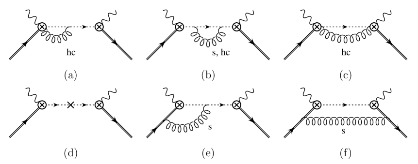
Figure 1: The one-loop SCET graphs contributing to the current correlator. Mirror graphs are not shown. Graph (d) shows the insertion of a counterterm from mass renormalization.

The calculation of the one-loop jet function is conceptually identical to that for the massless case [1, 2], and we will closely follow the treatment in [2]. The jet function is the matching coefficient between the hadronic tensor calculated in SCET and that calculated in HQET. The relevant SCET diagrams are shown in Fig.1. We calculate them in the parton model, using on-shell heavy quark states carrying a residual momentum $k$ satisfying $vk=0$. We work with dimensional regularization in $d=4-2\epsilon$ dimensions, using the Feynman gauge. The result for the graphs involving hard-collinear gluon exchange, including the counterterm from mass renormalization in the pole scheme (9), can be written as

$$D_{hc}^{(1)}=\mathcal{J}_{hc}^{(1)}\,\left[\bar{h}_{v}\,\bar{\Gamma}_{j}^{\mu}\,\frac{n\hskip-4.49997pt/_{-}}{2}\,\Gamma_{i}^{\nu}\,h_{v}\right],$$ (16)

where

$$\mathcal{J}_{hc}^{(1)} = \frac{C_{F}\alpha_{s}}{4\pi}\frac{i}{u^{\prime}}\Bigg{\{}\frac{4}{{\epsilon}^{2}}+\frac{3}{\epsilon}-\frac{4}{\epsilon}\ln\left(\frac{-n_{+}p\,u^{\prime}}{\mu^{2}}\right)$$ (17)

$$+ 7-\frac{{\pi}^{2}}{3}-3\,\ln\biggl{(}\frac{-n_{+}p\,u^{\prime}}{\mu^{2}}\biggr{)}+2\,\ln^{2}\biggl{(}\frac{-n_{+}p\,u^{\prime}}{\mu^{2}}\biggr{)}$$

$$+ \frac{2\,{\pi}^{2}}{3}-4\,\text{Li}_{2}\biggl{(}1+\frac{m_{p}}{u^{\prime}}\biggr{)}$$

$$+ \frac{m_{p}}{m_{p}+u^{\prime}}-\frac{m_{p}\,\left(m_{p}+2\,u^{\prime}\right)}{{\left(m_{p}+u^{\prime}\right)}^{2}}\,\ln\biggl{(}-\frac{u^{\prime}}{m_{p}}\biggr{)}\Bigg{\}}.$$

Here $u^{\prime}=u+n_{-}k$, $\alpha_{s}\equiv\alpha_{s}(\mu)$, and $m_{p}\equiv m_{c}^{2}/n_{+}p$. We have checked that our result (17) agrees with the corresponding result in [24] when expanded in $m_{c}^{2}/p^{2}$ and translated to the $\overline{\rm MS}$ scheme. The graphs involving soft gluon exchange give

$$D_{s}^{(1)}=\mathcal{J}_{s}^{(1)}\,\left[\bar{h}_{v}\,\bar{\Gamma}_{j}^{\mu}\,\frac{n\hskip-4.49997pt/_{-}}{2}\,\Gamma_{i}^{\nu}\,h_{v}\right],$$ (18)

where

$$\mathcal{J}_{s}^{(1)}=\frac{C_{F}\alpha_{s}}{4\pi}\frac{i}{u^{\prime}}\Bigg{\{}-\frac{2}{\epsilon^{2}}+\frac{2}{\epsilon}+\frac{4}{\epsilon}\ln\left(\frac{-{u^{\prime}}}{\mu}\right)-\frac{3\pi^{2}}{2}-4\ln\left(\frac{-{u^{\prime}}}{\mu}\right)-4\ln^{2}\left(\frac{-{u^{\prime}}}{\mu}\right)\Bigg{\}}.$$ (19)

The sum of the $1/\epsilon$ poles in $\mathcal{J}_{hc}^{(1)}+\mathcal{J}_{s}^{(1)}$ is removed by current renormalization in SCET, which is implemented by applying a factor of $Z_{J}^{2}$ (see 12) to the bare current correlator. This renormalization factor is related to the divergent part of the hard region of the QCD diagrams, which was integrated out in the first step of matching. That it cancels the $1/\epsilon$ poles from the SCET diagrams, which are due to both hard-collinear and soft regions, shows that we have indeed constructed the appropriate version of SCET. Moreover, the pole structure for each individual region is the same as in the massless case. It follows that the hard and shape functions obey the same renormalization group evolution as in the massless case, a fact which we will use when discussing decay distributions in the next section.

We can interpret the imaginary part of the finite pieces of the SCET diagrams as one-loop corrections to the factorized expression (15). They take the form $J^{(0)}\otimes S_{part}^{(1)}+J^{(1)}\otimes S_{part}^{(0)}$, where the superscript $(n)$ denotes the $n$-loop correction to each function, and the $\otimes$ stands for a convolution. The tree-level functions are $J^{(0)}=\delta(u-\omega)$ and $S^{(0)}_{part}=\delta(\omega+n_{-}k)$. As in the massless case, the one-loop correction to the shape function in the parton model is related to $\mathcal{J}_{s}^{(1)}$. To show this, we take its imaginary part, which can be expressed in terms of star distributions, defined as [25]

$$\int_{\leq 0}^{M}du\,F(u)\left(\frac{1}{u}\right)_{*}^{[m]} = \int_{0}^{M}du\frac{F(u)-F(0)}{u}+F(0)\ln\biggl{(}\frac{M}{m}\biggr{)},$$ (20)

$$\int_{\leq 0}^{M}du\,F(u)\left(\frac{\ln(u/m)}{u}\right)_{*}^{[m]} = \int_{0}^{M}du\frac{F(u)-F(0)}{u}\ln\frac{u}{m}+\frac{F(0)}{2}\ln^{2}\biggl{(}\frac{M}{m}\biggr{)}.$$ (21)

It is not difficult to derive the following formulas

$$-\frac{1}{\pi}{\rm Im}\left[\ln\left(-\frac{u}{m}\right)\frac{1}{u}\right]=\left(\frac{1}{u}\right)_{*}^{[m]}$$ (22)

$$-\frac{1}{\pi}{\rm Im}\left[\ln^{2}\left(-\frac{u}{m}\right)\frac{1}{u}\right]=2\left(\frac{\ln(u/m)}{u}\right)_{*}^{[m]}-\frac{\pi^{2}}{3}\delta(u),$$

where to take the correct branch of the logarithms we reinstored $u\equiv u+i\epsilon$. We then obtain

$$J^{(0)}\otimes S^{(1)}_{part}=S^{(1)}_{part}(u^{\prime})=\frac{1}{\pi}\text{Im}\biggl{[}i\,\mathcal{J}_{s,finite}^{(1)}\biggr{]}$$

$$=-\frac{C_{F}\alpha_{s}}{4\pi}\left[\frac{\pi^{2}}{6}\delta(u^{\prime})+4\biggl{(}\frac{1}{u^{\prime}}\biggr{)}_{*}^{\left[{\mu}\right]}+8\biggl{(}\frac{\ln(u^{\prime}\,/\mu)}{u^{\prime}}\biggr{)}_{*}^{\left[{\mu}\right]}\right],$$ (23)

which is identical to the one-loop result calculated in HQET. The jet function is related to the imaginary part of the finite piece of $\mathcal{J}_{hc}^{(1)}$ [2]. In particular, we have

$$J^{(1)}\otimes S^{(0)}_{part}=J^{(1)}(u^{\prime},n_{+}p)=\frac{1}{\pi}\text{Im}\biggl{[}i\,\mathcal{J}_{hc,finite}^{(1)}\biggr{]}.$$ (24)

Using (22) along with

$$-\frac{1}{\pi}\text{Im}\biggl{[}\frac{1}{u^{\prime}}\biggl{[}\text{Li}_{2}\biggl{(}1+\frac{m}{u^{\prime}}\biggr{)}\biggr{]}\biggr{]}=-\biggl{(}\frac{\ln(u^{\prime}\,/m)}{u^{\prime}}\biggr{)}_{*}^{\left[{m}\right]}+\frac{1}{u^{\prime}}\,\ln\biggl{(}1+\frac{u^{\prime}}{m}\biggr{)}\,\theta(u^{\prime}),$$ (25)

we find that the jet function to $\mathcal{O}(\alpha_{s})$ is given by

$$J(u^{\prime},n_{+}p)=\delta(u^{\prime}) + \frac{C_{F}\alpha_{s}}{4\pi}\biggl{\{}\left(7-\pi^{2}\right)\delta(u^{\prime})-3\biggl{(}\frac{1}{u^{\prime}}\biggr{)}_{*}^{\left[{\mu^{2}/n_{+}p}\right]}+4\biggl{(}\frac{\ln(u^{\prime}\,n_{+}p/\mu^{2})}{u^{\prime}}\biggr{)}_{*}^{\left[{\mu^{2}/n_{+}p}\right]}$$ (26)

$$+\biggl{(}\frac{u^{\prime}}{(m_{p}+u^{\prime})^{2}}-\frac{4}{u^{\prime}}\ln\biggl{(}1+\frac{u^{\prime}}{m_{p}}\biggr{)}\biggr{)}\,\theta(u^{\prime})+\left(1+\frac{{2\pi}^{2}}{3}\right)\,\delta(u^{\prime})$$

$$-\biggl{(}\frac{1}{u^{\prime}}\biggr{)}_{*}^{\left[{m_{p}}\right]}+4\,\biggl{(}\frac{\ln(u^{\prime}\,/m_{p})}{u^{\prime}}\biggr{)}_{*}^{\left[{m_{p}}\right]}\biggr{\}}.$$

The first line of (26) reduces to the result for the massless case in the limit $m_{c}\to 0$ [1, 2], while the second and third lines are unique to decay into charm quarks, and vanish for $m_{c}\to 0$.

We have also compared our calculation with the one-loop OPE result for $b\to c\ell\nu$ in [26]. For this purpose we re-expand the factorized expression for the hadronic tensor (15) in $\alpha_{s}$. Using the notation of [2], the component $W_{1}$ of the hadronic tensor, for instance, can be written as

$$\frac{W_{1}}{2} = \frac{1}{n_{+}p}\left[H_{\rm 11}\,\delta(u^{\prime})+J^{(1)}(u^{\prime},n_{+}p)+S^{(1)}_{\rm part}(u^{\prime})\right]+{\cal O}(\alpha_{s}^{2})\,,$$ (27)

where the soft and jet contribution are given in (23) and (26), and the hard contribution reads [2]

$$H_{\rm 11} = 1+\frac{\alpha_{s}C_{F}}{4\pi}\left(-4L^{2}+10L-4\ln y-\frac{2\ln y}{1-y}-4{\rm Li}_{2}(1-y)-\frac{\pi^{2}}{6}-12\right)$$ (28)

with $y=n_{+}p/m_{b}$ and $L=\ln\left[ym_{b}/\mu\right]$. This has to be compared with the corresponding expression in [26]

$$W_{3}^{\cite[cite]{[\@@bibref{}{Aquila:2005hq}{}{}]}} = \pi\,m_{b}^{2}\,W_{1}\,,$$ (29)

where the result for $W_{3}^{\cite[cite]{[\@@bibref{}{Aquila:2005hq}{}{}]}}$ has to be expanded, using the SCET power counting $m_{c}^{2}/m_{b}^{2}\sim\Lambda_{\rm QCD}/m_{b}\ll 1$. After some tedious, but straight-forward manipulations, we indeed find agreement with (27). The comparison for the remaining components $W_{4,5}$ of the hadronic tensor is much easier because at order $\alpha_{s}$ they receive contributions from the hard functions only. Therefore the limit $m_{c}/m_{b}\to 0$ in the corresponding expressions in [26] can be performed directly to recover the results for $W_{4,5}$ from [2].

4 The partially integrated $U$ spectrum

From the results of the previous section we can derive any differential decay distribution. We focus here on the $U$ spectrum, because of its relation to the $P_{+}$ spectrum from charmless decays. We pointed out in the last section that the hard and shape functions are unaffected by the presence of the charm-quark mass, and thus obey the same renormalization group equations as in the charmless case. In the remainder of the paper, we will work with the renormalization-group improved formulas derived in [2]. After integrating over the lepton energy and neglecting higher-order terms in $\lambda$, the doubly differential spectrum in the variables $u$ and $y$ is given by

$$\frac{1}{\Gamma_{c}}\,\frac{d^{2}\Gamma_{c}}{du\,dy}=e^{V_{H}(m_{b},\mu_{i})}\int_{-\bar{\Lambda}}^{u}d\omega\,y^{2-a}(6-4y)\,{\cal H}(y)\,J(u-\omega,m_{b}y,\mu_{i})\,S(\omega,\mu_{i})\,,$$ (30)

where $-\bar{\Lambda}\leq u\leq ym_{b}-m_{c}^{2}/ym_{b}$ and $m_{c}/m_{b}\leq y\leq 1$. Note that after resummation all of the functions are to be evaluated at the intermediate scale $\mu_{i}\sim m_{c}$. We have introduced the renormalization-group factors

$$a=\frac{16}{25}\ln\frac{\alpha_{s}(\mu_{i})}{\alpha_{s}(m_{b})},$$ (31)

and $V_{H}(m_{b},\mu_{i})$, which resum logarithms between the hard and the jet scale. The exact form of $V_{H}$ can be found in [2], and the hard function ${\cal H}$ can be derived from the functions $H_{ij}$ in the same reference. The total $b\to c$ rate to order $\alpha_{s}(m_{b})$ in the OPE is given by [29]

$$\Gamma_{c}=|V_{cb}|^{2}\left(\frac{G_{F}^{2}m_{b}^{5}}{192\pi^{3}}\right)\left[f\left(\frac{m_{c}^{2}}{m_{b}^{2}}\right)+\frac{C_{F}\alpha_{s}(m_{b})}{4\pi}\left(\frac{25}{2}-2\pi^{2}\right)g\left(\frac{m_{c}^{2}}{m_{b}^{2}}\right)\right].$$ (32)

At leading order in $\lambda$ we can set the phase-space factors $f,g$ to unity, although higher-order corrections may be important numerically, as we shall discuss in Section 4.

It is useful to change from partonic to hadronic variables and define

$$U=u+\bar{\Lambda},\qquad\hat{\omega}=\omega+\bar{\Lambda},\qquad\hat{S}(\hat{\omega})=S(\omega)\ .$$ (33)

The relation between the hadronic momenta $P^{\mu}$ and the partonic momenta $p^{\mu}$ is given by $n_{\pm}P=n_{\pm}p+\bar{\Lambda}$, where $\bar{\Lambda}=M_{B}-m_{b}$. This leads to

$$U = n_{-}P-\frac{m_{c}^{2}}{n_{+}P}+{\cal O}(\lambda^{4}).$$ (34)

To stay in the shape-function region, we need to restrict the phase-space integration to values of $U\sim\lambda^{2}m_{b}$. In order to preserve a close correspondence with the treatment of the $\bar{B}\to X_{u}\ell\bar{\nu}_{\ell}$ spectrum in [2], we introduce a cut $U<\Delta$, with $\Delta$ being around 600 MeV. The effect of this cut on the physical phase space in the variables $P_{-}=n_{+}P$ and $P_{+}=n_{-}P$ is illustrated in Fig. 2 for typical values $\Delta=0.65$ GeV and $m_{c}=1.36$ GeV. The fraction of events with $U<\Delta$ is then given by

$$F_{c}(\Delta) = \frac{\Gamma_{c}(U<\Delta)}{\Gamma_{c}}$$ (35)

$$= e^{V_{H}}\int_{0}^{\Delta}d\hat{\omega}\int_{\frac{m_{c}}{m_{b}}}^{1}dy\int_{0}^{\Delta}dU\,y^{2-a}(6-4y)\,{\cal H}(y)\,J(U-\hat{\omega},\,ym_{b})\,\hat{S}(\hat{\omega}).$$

A short calculation shows that the lower limit of the integration over $y$ can be set to zero, up to terms of order $(m_{c}/m_{b})^{3-a}$. After making this simplification, the integration limits are identical to those in $b\to u$ decays. In fact, the integrals over the $\alpha_{s}$ corrections from the hard function ${\cal H}$ and the first line of (26) are identical to the charmless case. We will give explicit results below.

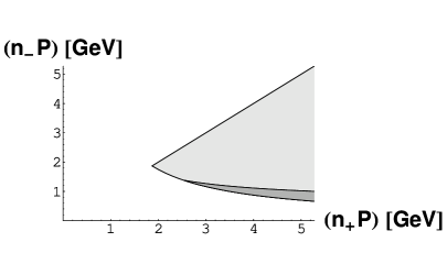
Figure 2: Illustration of the shape-function region singled out by the cut on the variable $U$. The light-grey region shows the physical phase space $M_{D}^{2}/n_{+}P\leq n_{-}P\leq n_{+}P\leq M_{B}$. The dark-grey part shows the shape-function region with $\Delta=0.65$ GeV and $m_{c}=1.36$ GeV.

The new terms relevant to decay into charm quarks are contained in the last two lines of (26). After integration over $U$ the result for these terms is

$$\begin{split}e^{V_{H}}\int_{0}^{\Delta}d\hat{\omega}\hat{S}(\hat{\omega})\int_{0}^{1}dy\,&y^{2-a}(6-4y)\frac{C_{F}\alpha_{s}(\mu_{i})}{4\pi}\bigg{\{}\frac{2\pi^{2}}{3}-\ln(y\Delta_{\hat{\omega}})+2\ln^{2}(y\Delta_{\hat{\omega}})\\ &+\frac{1}{1+y\,\Delta_{\hat{\omega}}}+\ln(1+y\Delta_{\hat{\omega}})+4\text{Li}_{2}(-y\Delta_{\hat{\omega}})\bigg{\}},\end{split}$$ (36)

where $\Delta_{\hat{\omega}}=(\Delta-\hat{\omega})m_{b}/m_{c}^{2}$. The integrals over $y$ can be evaluated in terms of the master integrals

$$G_{1}(n,x) = \int_{0}^{1}dy\,\frac{y^{n}}{1+xy}=\frac{{}_{2}F_{1}(1,n+1;n+2;-x)}{n+1},$$ (37)

$$G_{2}(n,x) = \int_{0}^{1}dy\,y^{n}\ln(1+xy)=\frac{1}{n+1}\left(\ln(1+x)-\frac{1}{n+1}\right)+\frac{G_{1}(n,x)}{n+1},$$ (38)

$$G_{3}(n,x) = \int_{0}^{1}dy\,y^{n}\text{Li}_{2}(-xy)=\frac{\text{Li}_{2}(-x)}{n+1}+\frac{G_{2}(n,x)}{n+1},$$ (39)

where the hypergeometric function ${}_{2}F_{1}$ has a series expansion

$${}_{2}F_{1}(a_{1},a_{2};a_{3};z)=\sum_{k=0}^{\infty}\frac{(a_{1})_{k}\,(a_{2})_{k}}{(a_{3})_{k}}\frac{z^{k}}{k!},\qquad(a_{i})_{k}=\frac{\Gamma(a_{i}+k)}{\Gamma(a_{i})}.$$ (40)

To express the final results in a compact way, we introduce

$$g_{n}(a,X) = \frac{6G_{n}(2-a,X)-4G_{n}(3-a,X)}{T(a)}\ ,$$ (41)

and make use of the functions defined in [2]

$$f_{2}(a) = -\frac{30-12a+a^{2}}{(6-a)(4-a)(3-a)},\qquad f_{3}(a)=\frac{2(138-90a+18a^{2}-a^{3})}{(6-a)(4-a)^{2}(3-a)^{2}},$$

$$T(a) = \frac{2(6-a)}{(4-a)(3-a)}\ .$$ (42)

The final result can be written as $F_{c}=F_{u}+F_{m}$. The fraction $F_{u}$ is the result for $b\to u$ decays

$$F_{u}(\Delta) = T(a)e^{V_{H}(m_{b},\mu_{i})}\int_{0}^{\Delta}d\hat{\omega}\,\hat{S}(\hat{\omega},\mu_{i})\,f_{u}\left(\frac{m_{b}(\Delta-\hat{\omega})}{\mu_{i}^{2}}\right)\ ,$$ (43)

$$f_{u}(x) = 1+\frac{C_{F}\alpha_{s}(m_{b})}{4\pi}H(a)$$

$$+\frac{C_{F}\alpha_{s}(\mu_{i})}{4\pi}\left[2\ln^{2}x+\big{(}4f_{2}(a)-3\big{)}\ln x+\big{(}7-\pi^{2}-3f_{2}(a)+2f_{3}(a)\big{)}\right].$$

An expression for $H(a)$ can be found in [2]. The fraction $F_{m}$ is an additional piece unique to decay into charm quarks, which vanishes when $m_{c}\to 0$. In the pole scheme, it is given by

$$F_{m}(\Delta) = T(a)\,e^{V_{H}(m_{b},\mu_{i})}\int_{0}^{\Delta}d\hat{\omega}\,\hat{S}(\hat{\omega},\mu_{i})\,f_{m}\left(\frac{m_{b}(\Delta-\hat{\omega})}{m_{c}^{2}}\right)\ ,$$ (44)

$$f_{m}(x) = \frac{C_{F}\alpha_{s}(\mu_{i})}{4\pi}\bigg{[}2\ln^{2}x+\big{(}4f_{2}(a)-1\big{)}\ln x$$

$$+\frac{2\pi^{2}}{3}-f_{2}(a)+2f_{3}(a)+g_{1}(a,x)+g_{2}(a,x)+4g_{3}(a,x)\bigg{]}\ .$$

From the partially integrated spectrum $F_{c}(\Delta)$ we can obtain the corresponding $U$ spectrum by differentiation, which results in

$$\frac{1}{\Gamma_{c}}\frac{d\Gamma_{c}}{dU} = T(a)\,e^{V_{H}(m_{b},\mu_{i})}\int_{0}^{U}d\hat{\omega}\left(\frac{d}{d\hat{\omega}}\hat{S}(\hat{\omega},\mu_{i})\right)\left[f_{u}\left(\frac{m_{b}(U-\hat{\omega})}{\mu_{i}^{2}}\right)+f_{m}\left(\frac{m_{b}(U-\hat{\omega})}{m_{c}^{2}}\right)\right]$$ (45)

where we have used integration by parts and $\hat{S}(0)=0$.

4.1 Change of charm-mass definition

So far, our analysis has been performed with $m_{c}$ defined in the pole scheme. The effect of changing the charm-mass definition according to

$$m_{c}\to\tilde{m}_{c}=m_{c}-\delta m\ ,$$

where $\delta m\sim m_{c}\alpha_{s}(\mu_{i})$, is two-fold. First, the input value for the charm-quark mass in $F_{m}(\Delta)$ is changed. Since the explicit charm-mass dependence in $F_{m}$ is already an ${\cal O}(\alpha_{s})$ correction, this effect is formally of order $\alpha_{s}^{2}$. Second, the jet function receives a perturbative correction proportional to $\delta m$. It can be obtained from the tree-level jet function by taking into account the appropriate shift in the spectral variable,

$$\delta(u-\omega) \simeq \delta\left(\tilde{u}-\omega\right)-\frac{2\tilde{m}_{c}\delta m}{n_{+}p}\,\delta^{\prime}(\tilde{u}-\omega),$$ (47)

where $\tilde{u}=n_{-}p-\tilde{m}_{c}^{2}/n_{+}p$ is defined using the new mass definition. Inserting the extra term into (35), one obtains an additional contribution to $F_{c}(\Delta)$,

$$F_{c}(\Delta) \to F_{c}(\Delta)-e^{V_{H}}\int_{0}^{\Delta}d\hat{\omega}\int_{0}^{1}dy\int_{0}^{\Delta}dU\,y^{2-a}(6-4y)\,\frac{2\tilde{m}_{c}\delta m}{ym_{b}}\,\delta^{\prime}(U-\hat{\omega})\,\hat{S}(\hat{\omega})$$ (48)

$$= F_{c}(\Delta)-e^{V_{H}}\,T(a+1)\,\frac{2\tilde{m}_{c}\delta m}{m_{b}}\,\hat{S}(\Delta)\ .$$

In order to see the scheme-independence of physical observables to a fixed order in $\alpha_{s}$, one has to keep in mind that the relation between the hadronic momenta and the spectral variable $U$ is also changed. Therefore, the result for $F_{c}(\Delta)$ in two different mass schemes should be compared at two different values of the cut-off parameter $\Delta$,

$$\tilde{U}=n_{-}P-\frac{\tilde{m}_{c}^{2}}{n_{+}P}\ <\ \tilde{\Delta}\simeq\Delta+\frac{2\tilde{m}_{c}\delta m}{n_{+}P}\ .$$ (49)

such that $\tilde{F}_{c}(\tilde{\Delta})$ in the new scheme reads

$$\tilde{F}_{c}(\tilde{\Delta}) = F_{u}(\tilde{\Delta})+F_{\tilde{m}}(\tilde{\Delta})-e^{V_{H}}\,T(a+1)\,\frac{2\tilde{m}_{c}\delta m}{m_{b}}\,\hat{S}(\tilde{\Delta})\ .$$ (50)

Expanding the upper limit $\tilde{\Delta}$ around $\Delta$ in the leading-order term in $F_{u}(\tilde{\Delta})$ and neglecting terms of order $\alpha_{s}^{2}$, we explicitly find the scheme-independence of our result,

$$\tilde{F}_{c}(\tilde{\Delta}) = F_{c}(\Delta)+{\cal O}(\alpha_{s}^{2})\ .$$ (51)

Still, the convergence of the perturbative series at a given value of $\Delta$ might be rather different for different mass definitions. In addition to the pole scheme, we will consider two further examples, namely

• the potential-subtracted (PS) scheme, where [30]

  $$m_{c}^{\rm PS}(\mu_{f}) = m_{c}-\frac{C_{F}\alpha_{s}(\mu_{i})}{\pi}\,\mu_{f}+{\cal O}(\alpha_{s}^{2})$$ (52)

  with $\mu_{f}\simeq 1$ GeV,

• the $\overline{\rm MS}$ scheme, where

  $$\bar{m}_{c}(\mu_{i}) = m_{c}\left[1+\frac{C_{F}\alpha_{s}(\mu_{i})}{4\pi}\left(3\ln\frac{m_{c}^{2}}{\mu_{i}^{2}}-4\right)+{\cal O}(\alpha_{s}^{2})\right]\ .$$ (53)

4.2 Numerical predictions

In this section we study the numerical predictions for $F_{c}(\Delta)$, taking into account mass-scheme and shape-function dependence. We start by summarizing the parameter values used in the subsequent analysis. The hard scale is fixed to the $b$-quark mass, $m_{b}=4.65$ MeV. The default value for the intermediate (jet) scale is $\mu_{i}=1.5$ GeV. We use the PS scheme as our default mass scheme, taking $m_{c}^{\rm PS}(\mu_{f}=1~{}{\rm GeV})=1.36$ GeV. The charm-quark pole mass is taken as $1.65$ GeV, and the $\overline{\rm MS}$ mass at the jet scale as $\bar{m}_{c}(\mu_{i})=1.20$ GeV. We use 2-loop running for $\alpha_{s}$ with $\Lambda_{\rm QCD}^{(n_{f}=4)}=345$ MeV, corresponding to $\alpha_{s}(m_{b})=0.22$ and $\alpha_{s}(\mu_{i})=0.37$.

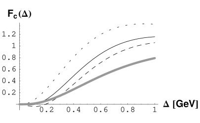
Figure 3: Predictions for partially integrated spectra in inclusive semi-leptonic $b\to c$ decays: Left: NLO prediction for $F_{c}(\Delta)$ using the the default scenario S5 [2] in the PS scheme (solid line) compared to the $\overline{\rm MS}$ scheme (long-dashed line) and the pole scheme (short-dashed line). Also plotted is the LO result (thick grey line). Right: NLO prediction for $F_{c}(\Delta)$ using the default scenario S5 in the PS scheme (solid line) compared to scenarios S1, S3, S7, S9 (dashed lines).

For the numerical estimate we have to specify a model for the shape function, which we take from [2]:

$$\hat{S}(\hat{\omega},\mu_{i}) = \frac{1}{\Lambda}\left[1-\frac{C_{F}\alpha_{s}(\mu_{i})}{4\pi}\left(\frac{\pi^{2}}{6}-1\right)\right]\,\frac{b^{b}}{\Gamma(b)}\left(\frac{\hat{\omega}}{\Lambda}\right)^{b-1}\exp\left(-b\frac{\hat{\omega}}{\Lambda}\right)\ .$$ (54)

We use $\Lambda=0.685$ GeV and $b=2.93$ as our default (scenario “S5” in [2]). In Fig. 3 we compare the results for different mass schemes and different input shape functions as a function of the cut-off $\Delta$. The following observations can be made:

• For values of $\Delta\sim 600$ MeV, the NLO corrections are large and positive.

• Above some critical value $\Delta_{\rm max}$, the NLO corrections become so large that the fraction $F_{c}$ exceeds 1, and therefore our result should not be trusted anymore.

• The critical value $\Delta_{\rm max}$ amounts to about $480$ MeV in the pole scheme, $700$ MeV in the PS scheme, and $860$ MeV in the $\overline{\rm MS}$ scheme.

• The model dependence from the input shape function amounts to an uncertainty of about 25%.

4.3 Power corrections

Figure 4: Effect of kinematic power corrections proportional to $\hat{S}(\hat{\omega})$: The curve shows the NLO prediction for $F_{c}(\Delta)$ including the power corrections to the tree-level result in (55), normalized to the leading-power result (43,44).

Our NLO calculation has been restricted to leading power in the $1/m_{b}$ expansion. Power corrections arise from two sources. First, one encounters new non-perturbative structure in the form of sub-leading shape functions. Second, there are kinematic power corrections proportional to $m_{c}^{2}/m_{b}^{2}\sim\lambda^{2}$ and $u\sim\lambda^{2}m_{b}$. The phase-space integration leads to logarithms $\ln(m_{c}^{2}/m_{b}^{2})$ which can numerically enhance some of the power-suppressed terms. Whereas the estimate of sub-leading shape function effects is model dependent, the kinematic corrections multiplying the leading-order shape function can be calculated explicitly. We shall do this at tree level only, where we can use the results of [16] to find

$$\frac{1}{\Gamma_{c}}\,\frac{d\Gamma_{c}}{dU} = \left\{1-\frac{U-\bar{\Lambda}}{m_{b}}\left(\frac{14}{3}+\frac{m_{c}^{2}}{m_{b}^{2}}\left(\frac{215}{6}+3\,\ln\frac{m_{c}^{2}}{m_{b}^{2}}\right)\right)+{\cal O}(u^{2},\lambda^{5})\right\}\hat{S}(U)$$ (55)

$${}+\mbox{sub-leading shape functions}\ .$$

The omitted terms are negligible in the portion of phase-space we are interested in. The numerical effect of the power corrections in (55) is plotted in Fig. 4. We see that $F_{c}(\Delta)$ is enhanced by about 20% at $\Delta=0.65$ GeV. Since we cannot control the remaining power corrections from sub-leading shape functions in a model-independent way, we consider this number as a rough estimate for the magnitude of the systematic uncertainties associated with power corrections.

5 Relating $b\to c$ and $b\to u$ decays

For the extraction of the CKM parameter $|V_{ub}|$ one would like to have a shape-function-independent relation between the $\bar{B}\to X_{u}\ell\bar{\nu}_{\ell}$ and $\bar{B}\to X_{c}\ell\bar{\nu}_{\ell}$ decay spectra. In what follows we focus on a relationship between the $P_{+}$ spectrum in $b\to u$ decays and the $U$ spectrum in $b\to c$ decays. This relation can be obtained in a similar way as discussed for the comparison of $\bar{B}\to X_{s}\gamma$ and $\bar{B}\to X_{u}\ell\bar{\nu}_{\ell}$ in [12]. In the present case, this involves constructing a weight function $W$ such that

$$\int_{0}^{\Delta}dP_{+}\,\frac{d\Gamma_{u}}{dP_{+}}=\frac{\Gamma_{u}}{\Gamma_{c}}\int_{0}^{\Delta}dU\,W(\Delta,U)\,\frac{d\Gamma_{c}}{dU}\simeq\frac{|V_{ub}|^{2}}{|V_{cb}|^{2}}\int_{0}^{\Delta}dU\,W(\Delta,U)\,\frac{d\Gamma_{c}}{dU},$$ (56)

where we have used that $\Gamma_{u}/\Gamma_{c}=|V_{ub}/V_{cb}|^{2}$ to leading power in $\lambda$. By measuring the partial decay rate $\Gamma_{u}(P_{+}<\Delta)$ in $b\to u$ decays, as well as the $d\Gamma_{c}/dU$ spectrum in $b\to c$ decays, we can determine $|V_{ub}|$. The theoretical input is the weight function $W$, which we can calculate from the results in (44,50):

$$W(\Delta,U) = 1-f_{m}\left(\frac{m_{b}(\Delta-U)}{(m_{c}^{\rm PS})^{2}}\right)+\frac{C_{F}\alpha_{s}(\mu_{i})}{4\pi}\frac{T(a+1)}{T(a)}\,\frac{8\mu_{f}m_{c}^{\rm PS}}{m_{b}}\,\delta(\Delta-U)$$ (57)

$${}+{\cal O}(\alpha_{s}^{2})+\mbox{power corrections},$$

in the PS scheme. We do not attempt to include power corrections here, but must be aware that they add a systematic uncertainty of at least 20%.

At the moment, we do not have explicit experimental information on the $U$ spectrum in $\bar{B}\to X_{c}\ell\bar{\nu}_{\ell}$, so to illustrate how our method works we will have to rely on some theoretical input. In the following subsections we will consider two approaches: In the first we will use the theoretical prediction (LABEL:eq:dGammac) for the $b\to c$ spectrum to obtain the $b\to u$ spectrum from the weight-function analysis with (57). In the second approach, we will construct a simple toy spectrum which takes into account possible charm-resonance effects.

5.1 Numerical analysis using theoretical $b\to c$ spectrum

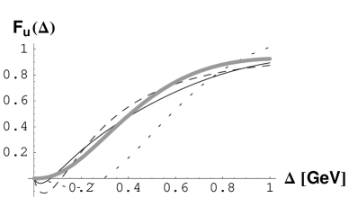
Figure 5: Predictions for $F_{u}(\Delta)$ using the weight function (57) and the theoretical $b\to c$ spectrum (LABEL:eq:dGammac) on the basis of the shape-function model S5 in (54). Solid line: PS scheme. Long-dashed line: $\overline{\rm MS}$ scheme. Short-dashed line: Pole scheme. For comparison, we also show the direct computation of $F_{u}(\Delta)$ from (43) (thick grey line).

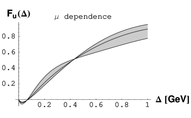
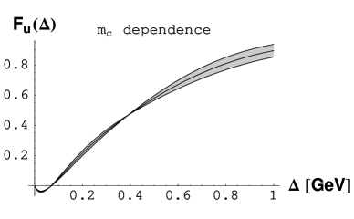
Figure 6: Predictions for $F_{u}(\Delta)$ using the weight function (57) and the theoretical $b\to c$ spectrum (LABEL:eq:dGammac) on the basis of the shape-function model S5 in (54). The left plot shows the scale dependence ($1$ GeV$<\mu_{i}<2.25$ GeV) of the result using the PS scheme. The right plot shows the effect of varying $m_{c}^{\rm PS}$ by $\pm 0.15$ GeV around its default value.

In this sub-section we carry out the weight-function analysis using the theoretical $b\to c$ spectrum from (LABEL:eq:dGammac) as input. This will help us estimate some of the perturbative uncertainties inherent to our approach. We start by constructing the partially integrated $b\to u$ spectrum $F_{u}(\Delta)$ from the theoretical $b\to c$ spectrum (LABEL:eq:dGammac) and the weight function $W(\Delta,U)$, using the shape-function model from (54). In Fig. 5 we compare the so-obtained results for $F_{u}(\Delta)$ in the PS, pole, and $\overline{\rm{MS}}$ schemes. We also show the result of the direct computation from (43). The difference between the curves is formally an ${\cal O}(\alpha_{s}^{2})$ effect, and thus gives a rough measure of higher-order perturbative effects. We observe that in the pole scheme this effect is quite large for values of $\Delta$ below $700$ MeV or so. At our reference point $\Delta=650$ MeV we obtain

$$F_{u}(0.65~{}{\rm GeV}) = 0.71\qquad\mbox{from (\ref{eq:dGammac}) and (\ref{eq:weight}), PS scheme}\ ,$$ (58)

$$F_{u}(0.65~{}{\rm GeV}) = 0.62\qquad\mbox{from (\ref{eq:dGammac}) and (\ref{eq:weight}), pole scheme}\ ,$$ (59)

$$F_{u}(0.65~{}{\rm GeV}) = 0.76\qquad\mbox{from (\ref{eq:dGammac}) and (\ref{eq:weight}), $\overline{\rm MS}$ scheme}\ ,$$ (60)

compared to

$$F_{u}(0.65~{}{\rm GeV}) = 0.79\qquad\mbox{from (\ref{eq:Fu})}\ ,$$ (61)

from which we deduce a residual scheme dependence for $F_{u}(\Delta)$ of about 10-15%.

In Fig. 6 we investigate the explicit $\mu_{i}$ and $m_{c}$ dependence induced by the weight function (to isolate these effects, we fix $m_{c}$ and $\mu_{i}$ in the theoretical expression (LABEL:eq:dGammac) for the $b\to c$ spectrum). The charm-mass dependence is a small effect, less than 10% for reasonably large values of $\Delta$. The dependence on the factorization scale $\mu_{i}$ is still sizeable, about 10-15%. The perturbative uncertainties related to the scheme and factorization-scale dependence could be resolved by calculating the $\alpha_{s}^{2}$ corrections to the jet function in the massive case.

5.2 Numerical analysis using a toy spectrum

The purpose of this sub-section is to point out some aspects of the weight-function analysis that would be important when dealing with the physical $b\to c$ spectrum. A distinctive feature of this spectrum is that that the lowest-lying spin-symmetry doublet of charmed states $D$ and $D^{*}$ already makes up about 80% of the semi-leptonic rate. For an on-shell $D(D^{*})$ meson we formally have

$$U_{D(D^{*})}=\frac{M_{D(D^{*})}^{2}-m_{c}^{2}}{n_{+}P}\ll\Delta\qquad(n_{+}P\sim m_{b})\ .$$ (62)

Therefore, about 80% of the $U$ spectrum is centered around “small” values of $U$ (we put “small” in quotation marks, because numerically $(M_{D}^{2}-m_{c}^{2})/m_{b}\simeq 350~{}$MeV in the PS scheme).

We will perform the weight-function analysis on a toy spectrum which takes this resonance structure into account. We construct this spectrum by assuming that the doubly-differential decay spectrum is concentrated along the $D/D^{*}$-pole and modulated by some function $f(y)$,

$$\frac{1}{\Gamma_{c}}\,\frac{d^{2}\Gamma_{c}}{d(n_{-}P)dy} \simeq \frac{m_{b}\,y^{2}}{\overline{M}_{D}^{2}}\,f(y)\,\delta\left(y-\frac{\overline{M}_{D}^{2}}{n_{-}P\,m_{b}}\right)\,$$ (63)

where $\int_{0}^{1}dy\,f(y)=1$, and $\overline{M}_{D}=1.975$ GeV is a weighted average of the $D$ and $D^{*}$ masses. We can derive the $U$ spectrum (in a given mass scheme) from this model by taking

$$n_{-}P=U+\frac{m_{c}^{2}}{ym_{b}}$$

and performing the integral over $y$, which yields

$$\frac{1}{\Gamma_{c}}\,\frac{d\Gamma_{c}}{dU} \simeq \frac{{\overline{M}}_{D}^{2}-m_{c}^{2}}{m_{b}U^{2}}\,f\left(\frac{{\overline{M}}_{D}^{2}-m_{c}^{2}}{m_{b}U}\right)\,\theta\left(U-\frac{\overline{M}_{D}^{2}-m_{c}^{2}}{m_{b}}\right)\,.$$ (64)

For the following discussion, we use a simple parameterization

$$f(y) = \frac{\Gamma(2+\alpha+\beta)}{\Gamma(1+\alpha)\Gamma(1+\beta)}\,y^{\alpha}\,(1-y)^{\beta}$$ (65)

and fix the parameters $\alpha=3.66$ and $\beta=-0.51$ by requiring that $F_{c}(\Delta)$ at $\Delta=650$ MeV, and $d\Gamma_{c}/dU$ at $U=550$ MeV coincide with the theoretical expressions in the PS scheme.

In Fig. 7 we compare the $U$ spectrum from our toy model with the theoretical prediction in the PS scheme, using the shape-function model (54) as input. Fig. 8 shows predictions for $F_{u}(\Delta)$ obtained by applying the weight-function analysis to our toy spectrum, as well as the theoretical curve obtained from (43). We see that at smaller values of $\Delta$ the sensitivity to the resonance structure and dependence on the mass scheme is sizeable. On the other hand, for larger values of $\Delta$ the resonance structure is washed out, and the predictions obtained in different mass schemes converge. The sensitivity to the resonance structure at moderate values of $\Delta$ means that the phenomenologically acceptable window for $\Delta$ in the shape-function approach is smaller than in the $b\to u$ case, where the contributions from the charmless ground states $\pi$, $\eta$, $\rho$ and $\omega$ add up to only about 25% of the total semi-leptonic $b\to u$ rate and are moreover centered at values of $P_{+}$ not much larger than 100 MeV.

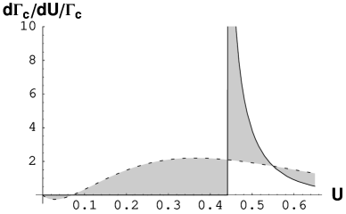
Figure 7: The $U$ spectrum in $\bar{B}\to X_{c}\ell\bar{\nu}_{\ell}$ decays: Theoretical prediction using the default model S5 for the shape function (dashed line) vs. phenomenological model (solid line) assuming the dominance of a single $D$-meson pole. The model parameters are adjusted to reproduce the value of the spectrum (left) at $U=550$ MeV as well as the integrated spectrum (right) at $\Delta=650$ MeV.

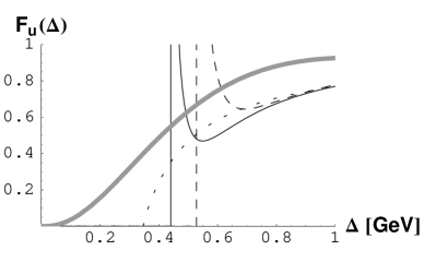
Figure 8: Predictions for the partial rate $F_{u}(\Delta)$ in $\bar{B}\to X_{u}\ell\bar{\nu}_{\ell}$ from a toy spectrum in $\bar{B}\to X_{c}\ell\bar{\nu}_{\ell}$ using the NLO weight function. Comparison of PS scheme (solid line), pole scheme (dotted), and $\overline{\rm MS}$ scheme (dashed) with the theoretical result (43) using scenario S5 (thick grey line).

These observations have important implications for extracting $|V_{ub}|$ by relating partially integrated $b\to u$ and $b\to c$ decay spectra. To apply our results to $b\to c$ decays, it is crucial that the cut-off parameter $\Delta$ be sufficiently large to avoid sensitivity to the shape of the spectrum in the resonance region. To apply them to $b\to u$ decays, $\Delta$ must be small enough to suppress the charm background, which sets in at $\Delta\sim 650$ MeV. Balancing between the two cases restricts the cut-off parameter $\Delta$ to a rather small window.

We also observe that the weight-function analysis with our toy model systematically underestimates the result for $F_{u}(\Delta)$ compared to the “true” result (43). For instance, at our reference point $\Delta=0.65$ GeV, we have

$$F_{u}(0.65~{}{\rm GeV}) = 0.79\qquad\mbox{from (\ref{eq:Fu})}\ ,$$ (66)

$$F_{u}(0.65~{}{\rm GeV}) = 0.55\qquad\mbox{from toy model and (\ref{eq:weight}), PS scheme}\ .$$ (67)

This is due at least in part to the crudeness of our model, which completely ignores the non-negligible continuum contribution. While we could refine our model to take this into account, we think that such fine-tuning is best resolved by experimental input.

6 Conclusions

We analyzed perturbative corrections to $\bar{B}\to X_{c}\ell\bar{\nu}_{\ell}$ decays using the power counting $m_{c}\sim\sqrt{\Lambda_{\rm QCD}m_{b}}$ for the charm-quark mass. This treatment implies that a certain class of partially integrated $b\to c$ decay spectra is sensitive to the non-perturbative shape-function effects familiar from $\bar{B}\to X_{u}\ell\bar{\nu}_{\ell}$ decays. With the aid of soft-collinear effective theory, we showed that the one-loop corrections to such decay spectra can be written as a convolution of hard, jet, and shape functions. The hard and shape functions are identical to those found in the factorization formula for $\bar{B}\to X_{u}\ell\bar{\nu}_{\ell}$ decays, but the jet function depends explicitly on $m_{c}$ and hence receives non-trivial corrections unique to decay into charm quarks. We calculated these corrections at NLO in perturbation theory and at leading order in the $1/m_{b}$ expansion, and derived a shape-function independent relation between partially integrated $\bar{B}\to X_{c}\ell\bar{\nu}_{\ell}$ and $\bar{B}\to X_{u}\ell\bar{\nu}_{\ell}$ decay spectra. This relation can be used to determine $|V_{ub}|$.

Numerical studies raised some issues related to this treatment. First, the portion of phase-space where the shape-function approach is valid is somewhat smaller in $\bar{B}\to X_{c}\ell\bar{\nu}_{\ell}$ decays than in the charmless case. Second, although the results are formally independent of the renormalization scheme used to define the charm-quark mass, the numerical dependence on the mass scheme is significant. Finally, the structure of power corrections is slightly more complicated than in the charmless case, since one encounters not only sub-leading shape functions, but also kinematic power corrections. Some of the power corrections are enhanced by large logarithms $\ln(m_{c}^{2}/m_{b}^{2})$.

Our study may help improve the understanding of inclusive $B$ decays in the shape-function region. On the one hand, it provides additional information for the extraction of $|V_{ub}|$. On the other hand, it may offer an additional testing ground for theoretical methods based on factorization and soft-collinear effective theory. To explore these ideas further would require experimental information on the partially integrated $\bar{B}\to X_{c}\ell\bar{\nu}_{\ell}$ decay spectrum used in our analysis.

References

- [1] C. W. Bauer and A. V. Manohar, Phys. Rev. D 70, 034024 (2004) [hep-ph/0312109].
- [2] S. W. Bosch, B. O. Lange, M. Neubert and G. Paz, Nucl. Phys. B 699, 335 (2004) [hep-ph/0402094].
- [3] K. S. M. Lee and I. W. Stewart, Nucl. Phys. B 721, 325 (2005) [hep-ph/0409045]; S. W. Bosch, M. Neubert and G. Paz, JHEP 0411, 073 (2004) [hep-ph/0409115]; M. Beneke, F. Campanario, T. Mannel and B. D. Pecjak, JHEP 0506, 071 (2005) [hep-ph/0411395].
- [4] M. Neubert, Eur. Phys. J. C 40 (2005) 165 [hep-ph/0408179].
- [5] K. S. M. Lee and I. W. Stewart, hep-ph/0511334.
- [6] M. Neubert, Phys. Rev. D 49, 3392 (1994) [hep-ph/9311325]; I. I. Y. Bigi, M. A. Shifman, N. G. Uraltsev and A. I. Vainshtein, Int. J. Mod. Phys. A 9, 2467 (1994) [hep-ph/9312359].
- [7] M. Neubert, Phys. Rev. D 49 (1994) 4623 [hep-ph/9312311].
- [8] T. Mannel and S. Recksiegel, Phys. Rev. D 60, 114040 (1999) [hep-ph/9904475].
- [9] A. K. Leibovich, I. Low and I. Z. Rothstein, Phys. Rev. D 61, 053006 (2000) [hep-ph/9909404].
- [10] S. W. Bosch, B. O. Lange, M. Neubert and G. Paz, Phys. Rev. Lett. 93, 221801 (2004) [hep-ph/0403223]; B. O. Lange, M. Neubert and G. Paz, Phys. Rev. D 72, 073006 (2005) [hep-ph/0504071].
- [11] A. H. Hoang, Z. Ligeti and M. Luke, Phys. Rev. D 71 (2005) 093007 [hep-ph/0502134].
- [12] B. O. Lange, M. Neubert and G. Paz, JHEP 0510, 084 (2005) [hep-ph/0508178].
- [13] B. O. Lange, JHEP 0601 (2006) 104 [hep-ph/0511098].
- [14] T. Mannel and M. Neubert, Phys. Rev. D 50, 2037 (1994) [hep-ph/9402288].
- [15] T. Mannel and F. J. Tackmann, Phys. Rev. D 71, 034017 (2005) [hep-ph/0408273].
- [16] H. Boos, T. Feldmann, T. Mannel and B. D. Pecjak, Phys. Rev. D 73 (2006) 036003 [hep-ph/0504005].
- [17] C. W. Bauer, S. Fleming and M. E. Luke, Phys. Rev. D 63, 014006 (2001) [hep-ph/0005275].
- [18] C. W. Bauer, S. Fleming, D. Pirjol and I. W. Stewart, Phys. Rev. D 63 (2001) 114020 [hep-ph/0011336].
- [19] C. W. Bauer, D. Pirjol and I. W. Stewart, Phys. Rev. D 65, 054022 (2002) [hep-ph/0109045].
- [20] M. Beneke, A. P. Chapovsky, M. Diehl and T. Feldmann, Nucl. Phys. B 643, 431 (2002) [hep-ph/0206152]; M. Beneke and T. Feldmann, Phys. Lett. B 553, 267 (2003) [hep-ph/0211358].
- [21] M. Beneke and V. A. Smirnov, Nucl. Phys. B 522 (1998) 321 [hep-ph/9711391].
- [22] I. Z. Rothstein, Phys. Rev. D 70 (2004) 054024 [hep-ph/0301240].
- [23] A. K. Leibovich, Z. Ligeti and M. B. Wise, Phys. Lett. B 564, 231 (2003) [hep-ph/0303099].
- [24] J. Chay, C. Kim and A. K. Leibovich, Phys. Rev. D 72, 014010 (2005) [hep-ph/0505030].
- [25] F. De Fazio and M. Neubert, JHEP 9906, 017 (1999) [hep-ph/9905351].
- [26] V. Aquila, P. Gambino, G. Ridolfi and N. Uraltsev, Nucl. Phys. B 719 (2005) 77 [hep-ph/0503083].
- [27] M. Trott, Phys. Rev. D 70 (2004) 073003 [hep-ph/0402120].
- [28] N. Uraltsev, Int. J. Mod. Phys. A 20 (2005) 2099 [hep-ph/0403166].
- [29] Y. Nir, Phys. Lett. B 221 (1989) 184.
- [30] M. Beneke, Phys. Lett. B 434 (1998) 115 [hep-ph/9804241].
- [31] C. W. Bauer, A. F. Falk and M. E. Luke, Phys. Rev. D 54 (1996) 2097 [hep-ph/9604290].