Quarkonia Correlators Above Deconfinement
Abstract
We study the quarkonia correlators above deconfinement using the potential model with screened temperature-dependent potentials. We find that while the qualitative features of the spectral functions, such as the survival of the 1S state, can be reproduced by potential models, the temperature dependence of the correlators disagree with the recent lattice data.
I Introduction
Current and past experiments at BNL and at CERN are and have been colliding heavy ions at relativistic velocities. One of the major goals of these experiments is to produce a deconfined state of matter, known as quark-gluon plasma. In this deconfined phase the dominant degrees of freedom are the different flavors of quarks and gluons which are not bound inside hadrons anymore. Unlike for light quarks, due to their smaller size, bound states of heavy quarks could survive inside the plasma to temperatures higher than that of deconfinement, . In the 1980’s, however, it was predicted Matsui:1986dk that bound states would disappear already at temperatures close to . The idea of Matsui and Satz, based on non-relativistic arguments, was that color screening in the plasma would prevent the strong binding of quarkonia. Therefore, the dissolution of heavy quark bound states, and thus the suppression of the peak in the dilepton spectra, could signal deconfinement.
It was recognized in the 1970’s Eichten:1979ms that what is now known as the Cornell potential (a Coulomb plus a linear part) provides a very good description of the quarkonia spectra at zero temperature. Much later it was understood that in non-relativistic systems, such as quarkonium, the hierarchy of energy scales ( and being the heavy quark mass and velocity), allows the construction of a sequence of effective theories : nonrelativistic QCD (NRQCD) and potential NRQCD (pNRQCD) Bali:2000gf ; yellow . The potential model appears as the leading order approximation of pNRQCD Bali:2000gf ; yellow , and thus can be derived in QCD from first principles.
The essence of the potential model calculations in the context of deconfinement is to use a finite temperature extension of the zero temperature Cornell potential to understand the modifications of the quarkonia properties at finite temperature Karsch:1987pv ; Digal:2001ue . It is not a priori clear though, whether the medium modifications of the quarkonia properties can be understood in terms of a temperature dependent potential. Therefore, a new way of looking at this problem has been developed. This new way is based on the evaluation on the lattice of the correlators and spectral functions of the heavy quark states Umeda:2002vr ; Asakawa:2003re ; Datta:2003ww . But why are correlators of heavy quarks of interest? As we said above, hadronic bound states are expected to dissolve at high temperatures. With increasing temperature such resonances become broader and thus very unstable and gradually it becomes meaningless to talk about them as being resonances. Accordingly, at and/or above they stop being the correct degrees of freedom. Correlation functions of hadronic currents, on the other hand, are meaningful above and below the transition. These can thus be used in a rather unambiguous manner to extract and follow the modification of the properties of quarkonia in a hot medium.
The numerical analysis of the quarkonia correlators and spectral functions carried out on the lattice for quenched QCD provided unexpected, yet interesting results Umeda:2002vr ; Asakawa:2003re ; Datta:2003ww . The results suggest the following: The ground state charmonia, 1S and , survive well above , at least up to . Not only do these states not melt at or close to as was expected, but lattice found little change in their properties when crossing the transition temperature. In particular, the masses of the 1S states show almost no thermal shift Umeda:2002vr ; Asakawa:2003re ; Datta:2003ww . Also, although the temperature dependence of the ground state quarkonium correlators was found to be small, a small difference between the behavior of the and the correlators has been identified. This difference was also not a priori expected. Furthermore, the lattice results indicate Datta:2003ww that properties of the 1P states, and , are significantly modified above the transition temperature, and these states have dissolved already at . The recently available first results for the bottomonia states Petrov:2005ej suggests, that the is not modified until about , but the shows dramatic changes already at .
These features from the lattice calculations are in sharp contrast with earlier, potential model studies of quarkonium properties at finite temperature, which predicted the dissolution of charmonia states for Karsch:1987pv ; Digal:2001ue . More recent studies try to resolve this apparent contradiction by choosing a potential which can bind the heavy quark anti-quark pair at higher temperatures. In Shuryak:2003ty the picture of strongly coupled Coulomb bound states is discussed. In Wong:2004zr ; Alberico:2005xw ; Mannarelli:2005pa the internal energy of a static quark anti-quark pair calculated on the lattice at finite temperature is used as the potential. It is found that the could be bound at temperatures as high as , in agreement with the lattice studies of the spectral functions. The quarkonium properties, however, are significantly modified in all of these calculations.
In connection with the potential models two questions should be addressed: First, can the medium modifications of quarkonia properties, and eventually their dissolution be understood in terms of a temperature dependent potential? Second, what kind of screened potential should be used in the Schrödinger equation, that describes well the bound states at finite temperature? At present neither of these questions have been answered, since it is not clear whether the sequence of effective theories leading to the potential model can be derived also at non-zero temperature, where the additional scales of order , and are present. Therefore, in this paper we follow a more phenomenological approach, extending our results presented in Mocsy:2004bv . We address the first question by constructing the heavy quarkonia correlators within the potential model and comparing them to the available lattice data. Our way of addressing the second question is to consider two different screened potentials and show that the qualitative conclusions do not depend on the specific choice of the potential. Our study of quarkonia correlators in Euclidean time is also motivated by the fact that although lattice calculations give very precise results about the temperature dependence of the quarkonia correlators (see e.g. Datta:2003ww ), it is quite difficult to reconstruct the spectral functions from the correlators at finite temperature.
The paper is organized as follows: Section II presents the model we use to construct the spectral function and analyze the correlators. In Section III our results for the temperature dependence of the quarkonia properties are presented. Section IV is devoted to the study of charmonium and bottomonium correlators in the scalar and pseudoscalar channels. In Section V we discuss the vector correlator which also carries information about diffusion properties. We summarize the results and present our conclusions in Section VI.
II Euclidean correlators and the potential model
Here we investigate the quarkonium correlators in Euclidean time at finite temperature, as these correlators are directly calculable in lattice QCD. To make contact with the available lattice data obtained in the quenched approximation, i.e. neglecting the effects of light dynamical quarks, we consider QCD with only one heavy quark flavor. Furthermore, we only consider the case of zero spatial momentum.
The correlation function for a particular mesonic channel is defined as
| (1) |
Here , and corresponds respectively to the scalar, vector, pseudoscalar and axial vector channels. At zero temperature these channels correspond to the different quarkonium states shown in Table 1.
| scalar | |||||
|---|---|---|---|---|---|
| pseudoscalar | |||||
| vector | |||||
| axial vector |
Using the Euclidean Hamiltonian (transfer matrix) the spectral decomposition of the correlators defined in Eq. (1) at zero temperature can be written as montvay
| (2) |
where the are the eigenstates of the Hamiltonian. For the few lowest lying states corresponds to the quarkonia masses, while the matrix elements give the decay constants. Furthermore, the Euclidean correlator is an analytic continuation of the real time correlator , , and the spectral function is
| (3) |
Here , and are the Fourier transforms of the real time correlators
| (4) | |||
| (5) |
and denotes the expectation value at finite temperature . Using the above, the following spectral representation for can be derived (see Appendix A)
| (6) |
where is the integration kernel
| (7) |
Recent lattice QCD calculations utilize the form (6) for the correlator to extract spectral functions. Results obtained with the Maximum Entropy Method are promising, but still somewhat controversial, and not fully reliable. We choose to directly analyze the correlators that are reliably calculated on the lattice. So as an input to (6) we need to specify the spectral function at finite temperature. We do this by following the form proposed in Shuryak:kg for the zero temperature spectral function
| (8) |
The first term contains the pole contributions from bound states (resonances), while the second term is the perturbative continuum above some threshold, denoted here by . While we know the asymptotic behavior of the spectral function from perturbation theory, no reliable information is available for the explicit form of the threshold function, . Therefore, in this work we consider two simple choices for it: First, we take the most simple form of , valid for free massless quarks, resulting in a sharp threshold. Then, we consider the form motivated by leading order perturbative calculations with massive quarks,
| (9) |
giving a smooth threshold. In leading order perturbation theory . The coefficients () were calculated at leading order in Karsch:2000gi , and are (-1,1), (1,0), (2,1), and (-2,3), for the scalar, pseudoscalar, vector, and axial vector channels, respectively 111The meson correlators in Karsch:2000gi differ by a factor of two from our definition.. Comparing the results obtained with these two forms of the threshold function gives us an estimate on the uncertainties resulting from the simplified form of the spectral function in equation (8).
In real QCD with three light quarks it is natural to identify the continuum threshold with the open charm or beauty threshold. For the case of one heavy quark only, which is considered here, the value of is somewhat arbitrary. Above some energy though, the spacing between the different states is so small that they eventually form a continuum. Parton-hadron duality then requires, that the area under the spectral function above this energy range is the same as the area under the free perturbative spectral function, justifying the form given above. This also motivates our choice of threshold as the energy above which no individual resonances are observed experimentally. The parameters of the zero temperature spectral function are given in Table 2.
| 0.471 | 0.192 GeV2 | 1.32 GeV | 4.746 GeV | 4.5 GeV | 11 GeV |
|---|
The remaining parameters of the spectral function (8) can be calculated using a potential model. The bound state masses are given by , where are the binding energies, and is the constituent mass of either the charm or the bottom quark. In order to calculate the decay constants , we first write the relativistic quark fields in terms of their non-relativistic components. This can be done using the Foldy-Wouthysen-Tani transformation
| (12) |
with being the spatial covariant derivative. At leading order in the coupling and inverse mass, the decay constant can be related to the wave function at the origin for the S states, i.e. the pseudoscalar and vector channel Bodwin:1994jh ,
| (13) |
and to the derivative of the wave function in the origin for P states, i.e. the scalar and axial-vector channels Bodwin:1994jh ,
| (14) |
where . For the number of colors we consider . The negative signs in Eq. (14) are the consequences of our definitions of the Euclidean Dirac matrices. For the derivation of these relations see Appendix B. To obtain the binding energies and the wave functions we solve the Schrödinger equation
| (15) |
with the Cornell potential
| (16) |
Here is the coupling and is the string tension. Their values, as well as the quark masses, were obtained in Jacobs:1986gv by fitting the zero temperature quarkonium spectrum. The parameters of the zero temperature analysis are summarized in Table 2. Note that the angular momentum in (15) distinguishes between the different quarkonium states shown in Table 1.
To model the binding and propagation of a heavy quark and antiquark in the deconfined phase, we assume that they interact via a temperature-dependent screened potential, and propagate freely above some threshold. Then, our finite temperature model spectral function has the form given in (8) with a now temperature-dependent decay constant, quarkonium mass, and threshold:
| (17) |
The last term in the spectral function is important at low frequencies and contributes at nonzero temperatures. It is present only in the vector channel, and is due to charge fluctuations and diffusion. The function for the scalar and the pseudoscalar states, and , for the vector channel. Since we consider the case of zero spatial momentum, there is no distinction between the transverse and the longitudinal components in the vector channel. Therefore, we sum over all four Lorentz components, . At nonzero spatial momentum, for , there would also be an additional contribution to the spectral function Karsch:2003wy . The charge susceptibility in the nonrelativistic approximation has the following form
| (18) |
The derivation of this expression, together with the full evaluation of the vector correlator at one-loop level is provided in the Appendix C. The relevance of this contribution in the spectral function for the possibility of obtaining transport coefficients from the lattice has been recently discussed in Petreczky:2005nh .
Just like at zero temperature, we calculate the binding energy and the wave function of the quarkonium states at finite temperature using the Schrödinger equation (15). For this we need to specify a temperature-dependent screened quark-antiquark potential. While the zero temperature potential can be calculated on the lattice, at nonzero temperature it is not clear how to define this quantity (for a discussion of this see Petreczky:2005bd ). Some ideas on how to generalize the notion of static potential to temperatures above deconfinement were presented in Simonov:2005jj . In the current analysis we use two different potentials: The screened Cornell potential above , first considered in Karsch:1987pv
| (19) |
The coupling and the string tension are specified in Table 2. We choose the following Ansatz for the temperature dependence of the screening mass GeV with GeV. This choice is motivated by the fact that we want to reproduce the basic observation from the lattice, namely that the 1S state exists up to , while the 1P state melts at . The potential (19) is shown in the left panel of Figure 1 for different temperatures above deconfinement.
In Shuryak:2003ty ; Wong:2004zr ; Alberico:2005xw the change in the internal energy induced by a static quark-antiquark pair, first calculated in Kaczmarek:2003dp , is used as the potential. This is a debatable choice of potential, since near the transition temperature the internal energy shows a very large increase Petreczky:2005bd ; Petreczky:2004pz ; Petreczky:2004xs . However, for temperatures we will also use the internal energy calculated on the lattice Kaczmarek:2003dp as the potential. We parameterize this as
| (20) |
This parameterization is shown against the actual lattice data in the right panel of Figure 1. The temperature dependence of the parameters of (20) is shown in Tables 5 and 6 in Appendix D.
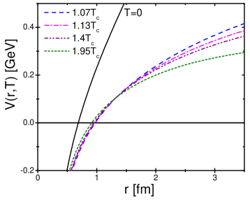
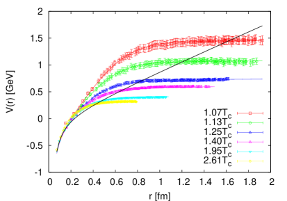
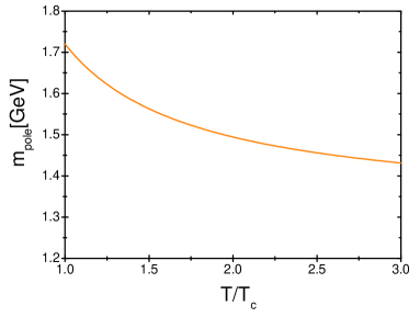
In the presence of screening the potential has a finite value at infinite separation (see Fig. 1). The is the extra thermal energy of an isolated quark. The minimum energy above which the quark-antiquark pair can freely propagate is . In what follows, we assume that this minimum energy defines the continuum threshold, i.e. . Independently of the detailed form of the potential, is decreasing, and thus will also decrease with temperature. This effect manifests in the temperature dependence of the correlators, as we will discuss in the following Section. Since at leading order the threshold of the continuum is , we may think of as the temperature dependent pole mass, shown in Fig. 2. The decrease of near can thus be considered as a decrease of the pole mass. Such a decrease of the pole mass was observed in lattice calculations Petreczky:2001yp , when calculating quark and gluon propagators in the Coulomb gauge. As the temperature increases the position of the peak will be close to the threshold, causing the phenomenon of threshold enhancement. This has recently been discussed for light quarks in Casalderrey-Solana:2004dc . We will not consider this in the present paper. While we assume that above the threshold quarks and antiquarks propagate with the temperature dependent effective mass defined above, quarks inside a singlet bound state will not feel the effect of the medium, and thus will have the vacuum mass. Therefore in the Schrödinger equation we use the zero temperature masses of the c and b quarks. Furthermore, above deconfinement quarkonium can also dissociate via its interaction with gluons Kharzeev:1994pz . This effect leads to a finite thermal width, which we will also neglect in the current analysis.
Finally, in order to make a direct comparison with the lattice results we normalize the correlation function by the so-called reconstructed correlators Datta:2003ww ; Petrov:2005ej . This is done to eliminate the trivial temperature dependence from the kernel (7) in the correlator (6). The reconstructed correlators are calculated using the spectral functions at a temperature below the critical one, here at :
| (21) |
The ratio can therefore indicate modifications to the spectral function above . Any difference of this ratio from one is an indication of the medium effects.
III Quarkonia properties above deconfinement
We first present the properties of the charmonia and bottomonia states in the deconfined medium. These results are obtained by solving the Schrödinger equation (15) with the screened Cornell potential (19).
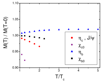
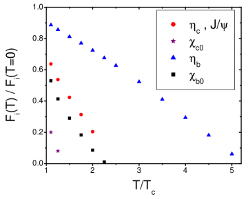
The temperature dependencies of the masses and the amplitudes of the different quarkonia states, normalized to their corresponding zero temperature values, are shown in Fig. 3. The left panel of Fig. 3 shows that the bound state masses do not change substantially with temperature. An exception is the mass of the scalar charmonium , which shows a significant decrease just above the transition temperature. The right panel of Fig. 3 shows the amplitudes, as obtained from the wave function, or its derivative at the origin. Contrary to the masses, these show a strong drop with increasing temperature for all the states considered. Since we neglect effects that could arise from the hyperfine splitting, the properties of the 1S scalar and pseudoscalar states are identical. While the small shift in the quarkonia masses above the deconfinement temperature is consistent with lattice data, the decrease in the amplitudes is neither confirmed, nor ruled out by existing lattice data.
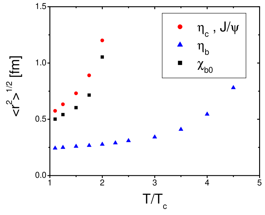
In Fig. 4 the temperature dependence of the radii is displayed. The radii of the scalar and pseudoscalar bottomonia states begin to increase at much higher temperatures than their corresponding charmonia states. This is expected, because bottomonia is much smaller in size, and therefore survives to much higher temperatures than charmonia. As the temperature increases and the screening radius decreases the effective size of a bound state becomes larger and larger, as seen in Fig. 4. When the size of the bound state is several times larger than the screening radius, thermal fluctuations can dissociate it. This means that the spectral functions no longer correspond to well defined bound states, but rather to some very broad structures. Here we consider a state to be melted, when its radius becomes greater than 1 fm. For this reason we do not show the radius of the , since it is significantly increased already at , suggesting the disappearance of this state at this temperature. Note, that the is similar in size to the and the , and shows significant increase of its radius at about the same temperature.
As mentioned in the previous Sections, several recent studies used the internal energy of a static quark-antiquark pair determined on the lattice as the potential in the Schrödinger equation to determine the properties of the quarkonia states at finite temperature. In the present study we also consider this possibility. The right panel in Figure 1 shows that close to the internal energy is significantly larger than its zero temperature value. Therefore, when used in the Schrödinger equation, this potential yields a large increase of the quarkonia masses and amplitudes near . The shift in the quarkonia masses is of the order of several hundred MeV, and thus disfavored by the lattice calculations of the quarkonia spectral functions.
The numerical values for the quarkonia properties, together with the temperature dependence of the parameters of the potential are given in the Appendix D. Tables 3 and 4 refer to the screened Cornell potential, and Tables 5 and 6 to the potential identified with the internal energy of a static quark-antiquark pair calculated on the lattice.
IV Numerical results for the Scalar and Pseudoscalar correlators
In this Section we discuss the results obtained for the temperature dependence of the correlators in the scalar and pseudoscalar quarkonia channels. We compare these to existing lattice results.
IV.1 Results with the Screened Cornell Potential
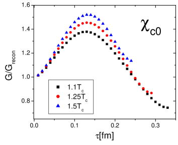
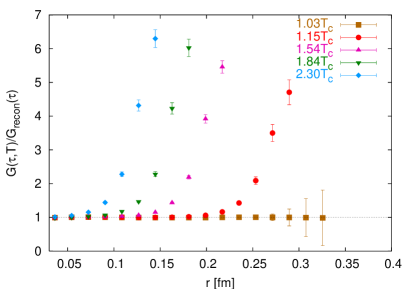
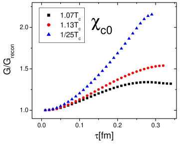
We present the temperature dependence of the scalar charmonia correlator, normalized to its reconstructed correlator in Fig. 5. The left panel displays the results obtained on the lattice Datta:2003ww . These show a very large increase of the correlator at , suggesting that the properties of the are already modified near the transition temperature. The potential model calculation using (19) as the potential, and a sharp threshold, i.e. in (17), with for the scalar, and for the pseudoscalar, are presented in the right panel.

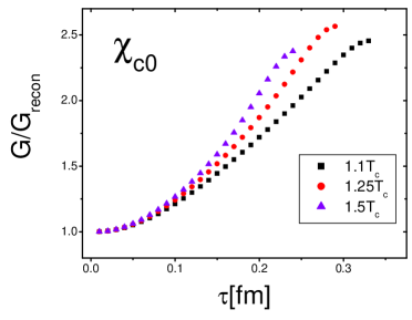
The calculated correlator shows an increase too, in qualitative agreement with the lattice data. Despite the fact that the contribution from the state becomes negligible, the scalar correlator above deconfinement is enhanced compared to the zero temperature correlator. This enhancement is due to the thermal shift of the continuum threshold .
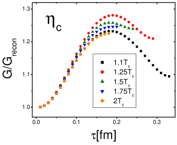
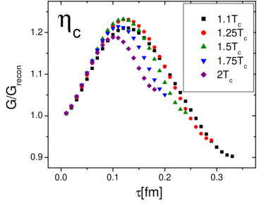
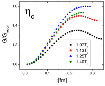
The pseudoscalar charmonia correlators are presented in Figure 6. The lattice correlator (left panel) shows no change until about , where a decrease is detected. The potential model with a sharp threshold (right panel), however, yields a moderate increase in the correlator at about fm. This feature is again attributed to the decrease of the continuum threshold with temperature, and is not detected on the lattice. After reaching a maximum drops, due to the decrease of the amplitude above deconfinement (c.f. Fig. 3).

We now discuss the results obtained with the smooth continuum threshold (9). The temperature dependence of the correlator obtained with the smooth threshold shows a somewhat different behavior, as seen in the left panel of Fig. 7. After enhancement at intermediate the correlator falls below the zero temperature one. We thus see that the temperature dependence of the scalar correlator is strongly affected by the continuum part of the spectral function. In this case too, the reduction of the continuum threshold clearly leads to the increase of the correlator at intermediate . When comparing the behavior of the correlator calculated with the sharp threshold (right panel in Fig. 6) and with the smooth threshold (9) (right panel of Fig. 7), we conclude that in the pseudoscalar channel although quantitatively the results are different, for the qualitative behavior only the reduction of the threshold, and not the exact form of the continuum matters.
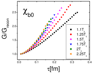
Qualitatively similar behavior was obtained for the bottomonia states. The scalar bottomonium correlator shown in Fig. 8 has an increase already at , as determined both on the lattice (left panel from Petrov:2005ej ) and in our model calculations (right panel). Here the sharp continuum has been used. Thus, the behavior of the scalar bottomonium channel is very similar to that of the scalar charmonium, even though, contrary to the state, the survives until much higher temperatures. We explain this with the fact, that the shifted continuum gives the dominant contribution to the scalar correlator.
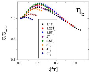
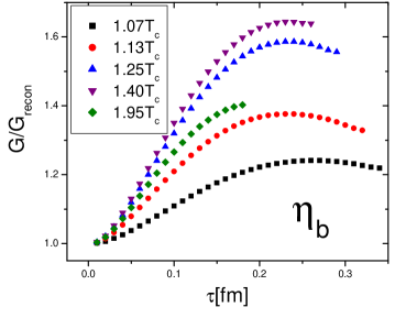
In Fig. 9 the behavior of the pseudoscalar bottomonium correlator is illustrated. Lattice results for this channel (left panel) show no deviation from one in the correlator ratio up to high temperatures. This is considered to be an indication of the temperature independence of the properties up to these temperatures. The potential model studies for the pseudoscalar correlator (right panel), yield again, a qualitatively different behavior than seen from the lattice. There is an increase at small , and a drop at large in the correlator compared to the zero temperature correlator. The increase is due to the threshold reduction, and the decrease is due to the reduction of the amplitude.

In summary, in this Section we have seen that for the pseudoscalar channel is increasing above one as the result of the shift in the continuum threshold, and its decrease is due to the decrease in the amplitude . This result is independent of the detailed form of the continuum. The temperature dependence of the scalar correlator is, on the other hand, sensitive to the continuum part of the spectral function.
IV.2 Results with Higher Excited States
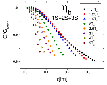
In the analysis presented so far we have considered only the lowest meson states in a given channel. We have done so, because we wanted to make contact with the existing lattice data, in which the excited states in any given channel were not yet identified. In order to study possible effects due to the higher states in a given channel, we now include also the 2S state, and the 2S and 3S states for the pseudoscalar charmonium, and bottomonium, respectively. These states enter directly in the first term of the spectral function (17). Since the 2S charmonium state is melted at (see Table 3 in Appendix D), we expect a larger drop in compared to the previous case, where only the 1S state is included. Similarly, the 3S bottomonium state is melted at , but the 2S state survives up until about (see Table 4 in Appendix D). The results are presented in Fig. 10. The left panel illustrates the temperature dependence of the correlator obtained when both the 1S and the 2S states are accounted for. As expected, we identify a 10%-20% reduction in the correlator, attributed to the melting of the 2S state. The lattice data on the pseudoscalar correlator shows no evidence for such a drop. Instead, within errors, up to . The right panel in Fig. 10 shows the correlator, where the melting of the 3S state near the transition, and the 2S state at higher temperatures, clearly induces a 10%-20% drop of the correlator compared to the case with only the 1S state included.
IV.3 Results Using the Internal Energy
We end this Section with the discussion of the quarkonia correlators obtained using as the potential the internal energy of a static quark-antiquark pair determined from the lattice. The temperature dependence of the correlators is illustrated in Fig. 11. In the numerical analysis we used the sharp continuum. As one can see from the left panels of Fig. 11 the behavior of the scalar correlator is similar to the one obtained in Section IV.1: Even though the and the states are dissociated, above the correlator is always enhanced relative to the zero temperature one. As shown on the right panels of Fig. 11 the enhancement in the pseudoscalar channel is larger than for the screened Cornell potential discussed in Section IV.1. As mentioned in Section III, the masses and amplitudes of the 1S quarkonia states calculated using the internal energy as the potential, show a significant increase at . The increase in the amplitudes translate into a significant enhancement of the correlators with respect to their values determined with the zero temperature amplitudes. Besides this increase due to the amplitude, our results prove to be qualitatively insensitive to the detailed form of the potential, suggesting that they are based on very general physical arguments. Thus we tested the robustness of our results regarding the discrepancy between potential model studies and lattice results.

V Numerical Results for the Vector correlator
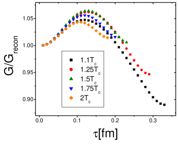
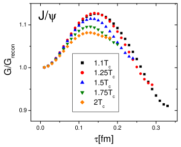
The vector correlator corresponds to an especially interesting channel. This is because of the fact, that the vector current is conserved. As mentioned in Section II (for the detailed analysis see Appendix C), this leads to an extra contribution in the spectral function compared to the scalar and pseudoscalar channels. This contribution (the third term in equation (17)) arises from the diffusion and charge fluctuations specific only for the vector state. Also, lattice data shows a difference in the temperature dependence of the pseudoscalar and the vector correlators. Namely, in the pseudoscalar channel the ratio is equal to one up to temperatures , and shows significant deviation at about , as illustrated on the left panel of Fig. 6. In the vector channel, shown in the left panel of Fig. 12, this ratio significantly decreases from one already at at distances fm. This figure further illustrates, that with increasing temperature the deviation happens already at smaller distances. Since to leading order in the non-relativistic expansion the pseudoscalar and vector channels correspond to the same 1S state, one would not expect the correlator of the and the to behave differently. Here we conjecture, that the effects of diffusion and charge fluctuations make the correlator smaller than the correlator of the .

The right panel of Fig. 12 displays the correlator from our potential model calculations. We see a rise of the correlator at small distances, where the continuum contribution to the spectral function is dominant, and thus again, the reduction of the threshold is manifest. As in the case of the pseudoscalar, the model calculations do not reproduce the behavior of the vector correlator obtained from the lattice. When comparing the and the correlator from the model calculations, i.e. the right panels of Figs. 6 and 12, at large distances we identify a reduction in the vector channel compared to the pseudoscalar channel, that results from diffusion and charge fluctuations.
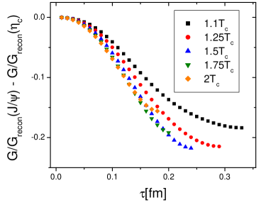
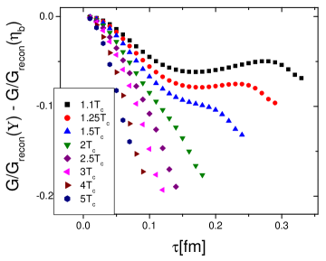
To better visualize the difference between the temperature dependence of the pseudoscalar and vector correlators, in Figure 13 we show the difference between the corresponding ratios for the charmonium (left panel) and the bottomonium (right panel) cases. From this figure one can clearly identify the drop in the correlator relative to the correlator. Similar to the charmonium case, for the bottomonium we also see a reduction at long distances of the correlator compared to the one. As expected, this reduction is more pronounced with increasing temperature, and for a given temperature is smaller for bottomonium than for charmonium.
VI Conclusions
In this work, we presented the first detailed study of the quarkonia properties and correlators using model spectral functions based on the potential picture with screening, and we contrasted these with lattice data. While the potential model with certain screened potentials can reproduce the qualitative features of the lattice data on the quarkonia spectral functions, namely the survival of the 1S state up to and dissociation of the 1P charmonia state at , the temperature dependence of the corresponding meson correlators is different from that seen on the lattice. In general, the temperature-dependencies of the correlators show much richer structure than those calculated on the lattice.
We identified several causes for the difference in the temperature dependence of the meson correlators: First, the properties of the different charmonia and bottomonia bound states, such as the masses and the wave functions, are significantly modified in the presence of screening, and will change the bound state contribution to the spectral function. Second, the behavior of the correlators is affected by the reduction of the continuum threshold. In a potential model with a screened potential the continuum threshold is related to the asymptotic value of the potential, which decreases with increasing temperature. Finally, the higher excited states (like the 2S, 3S, etc) are expected to melt at smaller temperatures above , inducing a large temperature dependence for the correlators.
What are the possible implications of these findings for the picture of quarkonium binding at finite temperature? It is possible that the effects of the medium on quarkonia binding cannot be understood in a simple potential model. The effects of screening, which according to lattice calculations are present in the plasma Petreczky:2005bd , could have time scales which are not small compared to the typical time scale of the heavy quark motion. In this case screening cannot affect significantly the properties of the quarkonia.
On the other hand, the implications of the finite temperature lattice data on quarkonia correlators also need to be reexamined. It is known that the high energy part of the quarkonia spectral functions is strongly influenced by lattice artifacts Datta:2003ww , resulting in the distortion of the continuum part of the quarkonia spectral functions. Furthermore, the excited states were not identified in the spectral functions determined on the lattice. Based on general physical arguments, though, one would expect the melting of the 2S charmonia and the 3S bottomonia states close to , together with the shift of the continuum, to induce a stronger temperature dependence of the correlators than actually observed in the lattice calculations. This statement is independent of whether or not the medium effects on quarkonia properties can be properly described in terms of potential models. In the future, therefore, this problem must be investigated in more detail.
Acknowledgements
We thank A. Dumitru, G. Moore, D. Teaney for discussions. We thank S. Datta for some of the lattice figures, and P. Sorensen for the careful reading of the manuscript. This work was partly supported by U.S. Department of Energy under contract DE-AC02-98CH10886. During the course of this work A. M. has been an Alexander von Humboldt Fellow, and P. P. has been a Goldhaber and is a RIKEN-BNL Fellow.
Appendix A Integral representation of the imaginary time correlator
Here we derive the spectral representation for the Euclidean correlator. We start from the Fourier decomposition of the real time two-point function
| (22) |
The Fourier transform is given in terms of the spectral function ,
| (23) |
with and lebellac . The Euclidean (Matsubara) propagator is an analytic continuation of the real time correlator
| (24) | |||||
| (25) |
Here we insert (23) and obtain
| (26) |
Now we perform a change of variables in the first term, and then use the identity together with the property of the spectral function, that this is an odd function in the frequency (the last relation is obtained from , which itself is derived from the periodicity in imaginary time, known as the Kubo-Martin-Schwinger relation lebellac ). We obtain
| (27) | |||||
Between the first and the second line above we inserted the identity . From (27) the final result for the Matsubara correlator is obtained:
| (28) |
Appendix B Bound State Amplitudes
Here we derive the different relationships between the decay constant of a given mesonic channel and the radial wave function, for the pseudoscalar and vector channels, or its derivative, for the scalar and axial vector channels (relations (13) and (14) in the main text).
The general idea is the following: We start from the definition of the correlator for the mesonic channel ,
| (29) |
where is the Euclidean time, and the are quark currents bilinear in the heavy quark field operator, that distinguishes between the scalar, vector, pseudoscalar and axial vector channels via and , respectively. Using the Foldi-Wouthuysen-Tani transformation we decouple the heavy quark and antiquark fields, reducing in this way the relativistic theory of Dirac spinors to a non-relativistic theory of Pauli spinors. Accordingly,
| (34) | |||||
| (39) |
and
| (42) |
Here is the quark field that annihilates a heavy quark, and the antiquark field that creates a heavy antiquark,
| (43) |
is the covariant derivative operator, the arrows indicate its direction of action. The Euclidean -matrices are given in the Dirac basis
being the Pauli matrices. Note, that for simplicity we suppressed the color and spin indexes on the quark field operators. We can rewrite the meson correlator in the form
| (44) |
where is an operator bilinear in the quark/antiquark fields. Its particular form will be discussed in the details that follow. Now using
| (45) |
and with the insertion of a complete set of states , where is an eigenstate of the Hamiltonian, , we derive a spectral representation for the correlator of the following form:
| (46) |
For large times, , the correlator is dominated by the state of lowest energy, and we can write
| (47) |
where and are the transition amplitude and the energy of the ground state. The amplitude is related to the decay constant, and can be directly related to the radial wave function, or its derivative, in the origin, as it was shown in Bodwin:1994jh . Following the steps described above let us now discuss the different channels separately.
-
•
We start with the pseudoscalar channel, since the calculation is simplest in this case. The current is
(48) (49) and to leading order in the inverse mass the correlator is
(50) At large the ground state dominates, and so
(51) where the refers to either of the or quarks. The relation to the wave function in the origin is provided by the equation (3.12a) from Bodwin:1994jh :
(52) Therefore, we can easily identify that
(53) -
•
The scalar current is
(54) After a straightforward, but tedious calculation, applying the relations of (43), and neglecting the disconnected piece, we get the following expression for the scalar correlator, to leading order in the inverse mass,
(55) Here the denotes the difference of the derivative acting on the spinor to the right and on the spinor to the left, . For large times the dominant contribution to the sum in (55) is from the lowest lying state, the . Utilizing equation (3.19b) from Bodwin:1994jh ,
(56) the relation between the amplitude and the derivative of the radial wave function at the origin is obtained for the , with ,
(57) The refers to the corresponding or quark mass.
-
•
Consider now the third component of the vector current:
(58) When inserting this into the correlator this yields for the diagonal components of this the following spectral decomposition:
(59) For the leading contribution to this correlator comes from the vector meson , and thus
(60) Equation (3.12b) from Bodwin:1994jh , with being the polarization vector of the vector meson, is
(61) Accordingly, the transition amplitude is
(62) and summing over all polarizations results in
(63) -
•
Finally, we turn to the axial vector channel. The ith component of the current is
(64) When evaluating the correlator we again make use of the cancellations of (43), and the anticommutativity of the quark field operators. Furthermore, we also apply the relation between the non-commuting Pauli matrices, , and the tensor notation of a vector product, . The resulting form of the correlator, when considering only , with , and neglecting the disconnected part, the grounds state, is
(65) Equation (3.19c) from Bodwin:1994jh relates the transition amplitude to the derivative of the wave function at the origin:
(66) We identify then the decay constant of an unpolarized axial vector channel to be
(67)
Appendix C Vector correlator at one-loop level
Here we derive the meson spectral function as obtained from the imaginary part of the retarded correlator. We will focus on the vector channel, since the spatial and the temporal component of its spectral function contain terms relevant for the analysis of the transport properties. The spectral function in the scalar, pseudoscalar and axial channels can be derived in an analogous manner.
The correlation function of a meson can be evaluated in momentum space, using the quark propagator and its spectral representation. Accordingly,
| (68) |
where is the number of colors, and refers to a given mesonic channel, defined by the operator for the scalar, pseudoscalar, vector, and axial-vector channels, respectively. Here , and . The quark propagator has the following form lebellac
| (69) |
Here is the free quark spectral function, with for a quark of mass . After inserting (69) into (68) and evaluating the integrals over the imaginary time , one obtains
| (70) | |||||
where for the second line we specified the vector correlator, .
First, let us evaluate the spatial part of (70), i.e consider and sum over the components:
| (71) | |||||
Here we inserted . Using standard techniques lebellac the Matsubara sums can be evaluated:
| (72) | |||||
where is the Fermi distribution function, with . In the following we introduce a small momentum approximations , according to which
| (73) | |||||
| (74) | |||||
| (75) | |||||
| (76) |
The spectral function is given by the imaginary part of the momentum space retarded correlation function, ,
| (77) |
We apply the relation
| (78) |
and obtain
| (81) | |||||
In the integrand for the limit of zero momentum, . The result for the spectral function at zero momentum is then
| (82) |
The first term is the leading order perturbative result for the continuum, also obtained in Karsch:2003wy . The second term provides a temperature-dependent contribution to the correlator. We evaluate this term in a non-relativistic approximation at the end of this Appendix.
Next, we evaluate the temporal part of the correlator. Inserting in (70) results in
| (83) | |||||
The corresponding component of the spectral function at small momentum is
| (85) | |||||
In the limit of zero momentum the contribution from the first term vanishes, and the final result is
| (86) | |||||
| (87) |
Here we identified the static charge susceptibility, , which can be evaluated explicitly. For heavy quarks the Fermi distribution function is well approximated by the Boltzmann distribution, , and thus
| (88) | |||||
| (89) |
where is the modified Bessel function of the second kind. Since the following approximation can be applied
| (90) |
yielding for the static susceptibility
| (91) |
Finally, we now evaluate the second contribution to (82), while incorporating a non-relativistic approximation for the heavy quarks. This means and . Thus
| (92) | |||||
Appendix D Numerical results as tables
Here we provide the results of the numerical calculations for the properties of the charmonia states, in Table 3, and bottomonia states, in Table 4, together with the temperature dependence of the screening mass in the screened Cornell potential, as well as the parameters of the potential fitted to the lattice internal energy and the charmonia properties in Tables 5 and 6.
| [GeV] | state | M[GeV] | [fm] | (S); (P) | |
| 0 | 0 | 1S | 3.07 | 0.453 | 0.735 GeV3 |
| 2S | 3.67 | 0.875 | 0.534 GeV3 | ||
| 1P | 3.5 | 0.695 | 0.06 GeV5 | ||
| 1.1 | 0.25 | 1S | 3.044 | 0.574 | 0.468 GeV3 |
| 2S | 3.338 | 1.591 | 0.137 GeV3 | ||
| 1P | 3.294 | 1.124 | 0.012 GeV5 | ||
| 1.25 | 0.314 | 1S | 3.031 | 0.633 | 0.395 GeV3 |
| 1P | 3.23 | 1.58 | 0.005 GeV5 | ||
| 1.5 | 0.395 | 1S | 3.012 | 0.73 | 0.311 GeV3 |
| 1P | 3.132 | 1.776 | 0.001 GeV5 | ||
| 1.75 | 0.472 | 1S | 2.992 | 0.89 | 0.23 GeV3 |
| 2 | 0.55 | 1S | 2.968 | 1.2 | 0.15 GeV3 |
| [GeV] | state | M[GeV] | [fm] | (S); (P) | |
| 0 | 0 | 1S | 9.445 | 0.225 | 9.422 GeV3 |
| 2S | 10.004 | 0.508 | 4.377 GeV3 | ||
| 1P | 9.897 | 0.407 | 1.39 GeV5 | ||
| 3S | 10.355 | 0.74 | 3.42 GeV3 | ||
| 2P | 10.259 | 0.65 | 1.74 GeV5 | ||
| 1.1 | 0.25 | 1S | 9.52 | 0.243 | 8.346 GeV3 |
| 2S | 9.945 | 0.641 | 2.632 GeV3 | ||
| 1P | 9.893 | 0.501 | 0.738 GeV5 | ||
| 2P | 10.092 | 0.95 | 0.54 GeV5 | ||
| 1.25 | 0.314 | 1S | 9.536 | 0.249 | 8.07 GeV3 |
| 2S | 9.924 | 0.695 | 2.195 GeV3 | ||
| 1P | 9.885 | 0.541 | 0.574 GeV5 | ||
| 2P | 10.041 | 1.13 | 0.32 GeV5 | ||
| 1.5 | 0.395 | 1S | 9.553 | 0.259 | 7.644 GeV3 |
| 2S | 9.895 | 0.806 | 1.676 GeV3 | ||
| 1P | 9.872 | 0.603 | 0.404 GeV5 | ||
| 1.75 | 0.472 | 1S | 9.569 | 0.267 | 7.257 GeV3 |
| 2S | 9.864 | 0.974 | 1.096 GeV3 | ||
| 1P | 9.854 | 0.715 | 0.255 GeV5 | ||
| 2 | 0.55 | 1S | 9.582 | 0.277 | 6.818 GeV3 |
| 2S | 9.832 | 1.246 | 0.627 GeV3 | ||
| 1P | 9.832 | 1.053 | 0.12 GeV5 | ||
| 2.25 | 0.628 | 1S | 9.594 | 0.289 | 6.369 GeV3 |
| 1P | 9.802 | 2.404 | 0.015 GeV5 | ||
| 2.5 | 0.705 | 1S | 9.603 | 0.309 | 5.867 GeV3 |
| 3 | 0.86 | 1S | 9.618 | 0.342 | 4.923 GeV3 |
| 3.5 | 1.015 | 1S | 9.627 | 0.41 | 3.865 GeV3 |
| 4 | 1.17 | 1S | 9.63 | 0.545 | 2.771 GeV3 |
| 4.5 | 1.325 | 1S | 9.628 | 0.78 | 1.707 GeV3 |
| 5 | 1.48 | 1S | 9.62 | 2.146 | 0.578 GeV3 |
| [GeV]2 | [GeV] | [GeV] | state | M[GeV] | [fm] | (S); (P) | |
| 0 | 0.18 | 0 | 0 | 1S | 3.177 | 0.500 | 0.441 GeV3 |
| 2S | 3.733 | 0.923 | 0.370 GeV3 | ||||
| 1P | 3.534 | 0.733 | 0.034 GeV5 | ||||
| 1.07 | 0.0417 | 0.123 | 1.467 | 1S | 3.522 | 0.399 | 0.863 GeV3 |
| 1P | 4.059 | 0.791 | 0.072 GeV5 | ||||
| 1.13 | 0.0484 | 0.155 | 1.09 | 1S | 3.448 | 0.458 | 0.688 GeV3 |
| 1.25 | 0.074 | 0.193 | 0.747 | 1S | 3.448 | 0.636 | 0.411 GeV3 |
| [GeV]2 | [GeV] | [GeV] | state | M[GeV] | [fm] | (S); (P) | |
| 0 | 0.181 | 0 | 0 | 1S | 9.693 | 0.283 | 3.477 GeV3 |
| 2S | 10.115 | 0.567 | 2.268 GeV3 | ||||
| 3S | 10.419 | 0.797 | 1.949 GeV3 | ||||
| 1P | 9.996 | 0.452 | 0.539 GeV5 | ||||
| 2P | 10.315 | 0.701 | 0.773 GeV5 | ||||
| 1.07 | 0.074 | 0.131 | 1.471 | 1S | 9.839 | 0.227 | 5.590 GeV3 |
| 2S | 10.544 | 0.454 | 3.932 GeV3 | ||||
| 3S | 10.930 | 0.927 | 1.508 GeV3 | ||||
| 1P | 10.318 | 0.346 | 1.775 GeV5 | ||||
| 2P | 10.826 | 0.630 | 1.742 GeV5 | ||||
| 1.13 | 0.087 | 0.161 | 1.094 | 1S | 9.827 | 0.234 | 5.267 GeV3 |
| 2S | 10.435 | 0.530 | 2.829 GeV3 | ||||
| 1P | 10.266 | 0.377 | 1.369 GeV5 | ||||
| 1.25 | 0.134 | 0.174 | 0.752 | 1S | 9.826 | 0.236 | 5.136 GeV3 |
| 2S | 10.435 | 0.530 | 2.771 GeV3 | ||||
| 1P | 10.266 | 0.376 | 1.475 GeV5 | ||||
| 1.40 | 0 | 0.408 | 0.608 | 1S | 9.820 | 0.258 | 4.695 GeV3 |
| 1.95 | 0 | 0.313 | 0.611 | 1S | 9.864 | 0.388 | 3.216 GeV3 |
References
- (1) T. Matsui and H. Satz, Phys. Lett. B 178, 416 (1986).
- (2) E. Eichten, K. Gottfried, T. Kinoshita, K. D. Lane and T. M. Yan, Phys. Rev. D 21, 203 (1980).
- (3) G. S. Bali, Phys. Rept. 343, 1 (2001) [arXiv:hep-ph/0001312].
- (4) N. Brambilla et al, Quarkonium Physics, CERN Yellow Report, hep-ph/0412158
- (5) F. Karsch, M. T. Mehr and H. Satz, Z. Phys. C 37, 617 (1988).
- (6) S. Digal, P. Petreczky and H. Satz, Phys. Rev. D 64, 094015 (2001) [arXiv:hep-ph/0106017].
- (7) T. Umeda, K. Nomura and H. Matsufuru, Eur. Phys. J. C 39S1, 9 (2005) [arXiv:hep-lat/0211003].
- (8) M. Asakawa and T. Hatsuda, Phys. Rev. Lett. 92, 012001 (2004) [arXiv:hep-lat/0308034].
- (9) S. Datta, F. Karsch, P. Petreczky and I. Wetzorke, Phys. Rev. D 69, 094507 (2004) [arXiv:hep-lat/0312037].
- (10) K. Petrov, A. Jakovác, P. Petreczky and A. Velytsky, arXiv:hep-lat/0509138.
- (11) E. V. Shuryak and I. Zahed, Phys. Rev. C 70, 021901 (2004) [arXiv:hep-ph/0307267]; Phys. Rev. D 70, 054507 (2004) [arXiv:hep-ph/0403127].
- (12) C. Y. Wong, arXiv:hep-ph/0408020.
- (13) W. M. Alberico, A. Beraudo, A. De Pace and A. Molinari, arXiv:hep-ph/0507084.
- (14) M. Mannarelli and R. Rapp, arXiv:hep-ph/0509310.
- (15) Á. Mócsy and P. Petreczky, Eur. Phys. J. C 43, 77 (2005) [arXiv:hep-ph/0411262]; arXiv:hep-ph/0510135.
- (16) I. Montvay, G. Münster, Quantum Fields on a Lattice, Cambridge University Press, 1996.
- (17) E. V. Shuryak, Rev. Mod. Phys. 65, 1 (1993).
- (18) F. Karsch, M. G. Mustafa and M. H. Thoma, Phys. Lett. B 497, 249 (2001) [arXiv:hep-ph/0007093].
- (19) G. T. Bodwin, E. Braaten and G. P. Lepage, Phys. Rev. D 51, 1125 (1995) [Erratum-ibid. D 55, 5853 (1997)] [arXiv:hep-ph/9407339].
- (20) Y. A. Simonov, Phys. Lett. B 619, 293 (2005) [arXiv:hep-ph/0502078].
- (21) S. Jacobs, M. G. Olsson and C. I. Suchyta, Phys. Rev. D 33, 3338 (1986) [Erratum-ibid. D 34, 3536 (1986)].
- (22) P. Petreczky and D. Teaney, arXiv:hep-ph/0507318.
- (23) P. Petreczky, Eur. Phys. J. C 43, 51 (2005) [arXiv:hep-lat/0502008].
- (24) O. Kaczmarek, F. Karsch, P. Petreczky and F. Zantow, Nucl. Phys. Proc. Suppl. 129, 560 (2004) [arXiv:hep-lat/0309121].
- (25) P. Petreczky and K. Petrov, Phys. Rev. D 70, 054503 (2004) [arXiv:hep-lat/0405009].
- (26) P. Petreczky, Nucl. Phys. Proc. Suppl. 140, 78 (2005) [arXiv:hep-lat/0409139].
- (27) P. Petreczky, F. Karsch, E. Laermann, S. Stickan and I. Wetzorke, Nucl. Phys. Proc. Suppl. 106, 513 (2002) [arXiv:hep-lat/0110111].
- (28) J. Casalderrey-Solana and E. V. Shuryak, arXiv:hep-ph/0408178.
- (29) D. Kharzeev and H. Satz, Phys. Lett. B 334, 155 (1994) [arXiv:hep-ph/9405414].
- (30) M. le Bellac: Thermal Field Theory, Cambridge University Press, 1996.
- (31) F. Karsch, E. Laermann, P. Petreczky and S. Stickan, Phys. Rev. D 68, 014504 (2003) [arXiv:hep-lat/0303017].