Range of validity of
transport equations

Transport equations can be derived from quantum field theory assuming a loss of information about the details of the initial state and a gradient expansion. While the latter can be systematically improved, the assumption about a memory loss is in general not controlled by a small expansion parameter. We determine the range of validity of transport equations for the example of a scalar $g^{2}\Phi^{4}$ theory. We solve the nonequilibrium time evolution using the three-loop 2PI effective action. The approximation includes off-shell and memory effects and assumes no gradient expansion. This is compared to transport equations to lowest order (LO) and beyond (NLO). We find that the earliest time for the validity of transport equations is set by the characteristic relaxation time scale $t_{\rm damp}=-2\omega/\Sigma^{\rm(eq)}_{\varrho}$, where $-\Sigma^{\rm(eq)}_{\varrho}/2$ denotes the on-shell imaginary-part of the self-energy. This time scale agrees with the characteristic time for partial memory loss, but is much shorter than thermal equilibration times. For times larger than about $t_{\rm damp}$ the gradient expansion to NLO is found to describe the “full” results rather well for $g^{2}\lesssim 1$.

1 Introduction

Important phenomena in high-energy physics related to collision experiments of heavy nuclei, early universe cosmology and other complex many-body systems urge a quantitative understanding of nonequilibrium dynamics in quantum field theories. One of the most crucial aspects concerns the characteristic time scales on which thermal equilibrium is approached. Much of the recent interest derives from observations in collision experiments of heavy nuclei at RHIC. The experiments seem to indicate early thermalization, whereas the present theoretical understanding of QCD suggests a significantly longer thermal equilibration time [1].

Most theoretical estimates concerning the important question of thermalization have been obtained from transport theory, or assuming in addition a quasi-particle picture, from kinetic theory. Transport equations can be derived from quantum field theory assuming a loss of information about the details of the initial state and a gradient expansion. While the latter can be systematically improved, the assumption about a memory loss is in general not controlled by a small expansion parameter. The time for a (partial) loss of memory represents a minimum characteristic time after which transport descriptions may be applied. It is important to quantify this characteristic time in quantum field theory. The question is whether transport or kinetic theory can be used to quantitatively describe the early-time behavior, which is necessary if their application to the problem of fast apparent thermalization is viable.

With the advent of new computational techniques a direct account of quantum field degrees of freedom becomes increasingly feasible. There has been important progress in our understanding of nonequilibrium quantum fields using suitable resummation techniques based on 2PI generating functionals [2]. They have been successfully used to describe far-from-equilibrium dynamics and subsequent thermalization in quantum field theory [3, 4, 5, 6, 7, 8]. While it is difficult to test analytic approximations for theories such as QCD, where strong interactions play an important role, the description of scalar and fermionic theories for not too strong couplings seems well under quantitative control by now.

In this work we determine the range of applicability of transport equations for a scalar $g^{2}\Phi^{4}$ theory. The latter has been frequently studied in the past using the required 2PI loop- [9] or 2PI $1/N$-expansions beyond lowest order [4, 10]. Here we employ a three-loop 2PI effective action in $3+1$ dimensions. It includes direct scatterings, off-shell and memory effects. Most importantly in this context, it employs no derivative expansion or quasi-particle assumption. We solve the nonequilibrium evolution for a class of nonequilibrium initial conditions reminiscent of some aspects of the anisotropic initial stage in the central region of two colliding wave packets.

We then derive the corresponding transport equations to lowest order (LO) and next-to-lowest order (NLO) following standard prescriptions. Both LO and NLO are then compared to the “full” results as described in Sec. 4. It turns out that the NLO corrections are crucial already for relatively small couplings, which made it necessary to go beyond the LO study presented in Ref. [11]. The LO expressions are typically employed to obtain kinetic or Boltzmann equations using in addition a quasi-particle approximation. We emphasize that our comparisons do not rely on any kind of quasi-particle ansatz. We concentrate on the applicability of transport theory based on a derivative expansion, which also provides the necessary condition for the applicability of kinetic equations.

2 Exact evolution equations

We start by considering the exact nonequilibrium evolution equation for the time-ordered two-point correlation function

$$G(x,y) = \langle T\Phi(x)\Phi(y)\rangle$$ (2.1)

$$\equiv F(x,y)-\frac{i}{2}\rho(x,y)\,{\rm sign}(x^{0}-y^{0})\,,$$

i.e. the expectation value of the product of two Heisenberg field operators $\Phi$ with time-ordering $T$. Here $\langle\ldots\rangle$ includes the trace over the density matrix describing the initial state [2]. For simplicity, we will consider a scalar $g^{2}\Phi^{4}$ field theory in the symmetric regime where the field expectation value vanishes, i.e. $\langle\Phi(x)\rangle=0$.

In general, there are two independent two-point functions, which can be associated to the commutator and anti-commutator of two fields. Accordingly, the second line in Eq. (2.1) is a rewriting, which expresses the time-ordered product using

$$\rho(x,y) = i\langle[\Phi(x),\Phi(y)]\rangle\,,$$ (2.2)

$$F(x,y) = \frac{1}{2}\langle\{\Phi(x),\Phi(y)\}\rangle\,.$$ (2.3)

Here $\rho(x,y)$ denotes the spectral function and $F(x,y)$ the statistical two-point function. For the real scalar theory these determine the imaginary part and the real part of the two-point function (2.1), respectively. While the spectral function encodes the spectrum of the theory, the statistical propagator gives information about occupation numbers. Loosely speaking, the decomposition (2.1) makes explicit what states are available and how often they are occupied. For nonequilibrium, $F(x,y)$ and $\rho(x,y)$ are in general two independent real-valued two-point functions. A simplification occurs in vacuum or thermal equilibrium where $F(x,y)$ and $\rho(x,y)$ are related by the fluctuation-dissipation relation [6]. We note that the spectral function encodes the equal-time commutation relations:

$$\rho(x,y)|_{x^{0}=y^{0}}=0\quad,\quad\partial_{x^{0}}\rho(x,y)|_{x^{0}=y^{0}}=\delta({\vec{x}}-{\vec{y}})\,.$$ (2.4)

The exact evolution equations for the statistical and spectral functions read (for a detailed derivation see e.g. [2]):

$$\left[\square_{x}+M^{2}(x)\right]F(x,y) = -\int_{0}^{x^{0}}\!{\rm d}z^{0}\int_{-\infty}^{\infty}\!{\rm d}^{d}z\,\Sigma_{\rho}(x,z)F(z,y)$$ (2.5)

$$+\int_{0}^{y^{0}}\!{\rm d}z^{0}\int_{-\infty}^{\infty}\!{\rm d}^{d}z\,\Sigma_{F}(x,z)\rho(z,y)\,,$$

$$\left[\square_{x}+M^{2}(x)\right]\rho(x,y) = -\int_{y^{0}}^{x^{0}}\!{\rm d}z^{0}\int_{-\infty}^{\infty}\!{\rm d}^{d}z\,\Sigma_{\rho}(x,z)\rho(z,y)\,.$$ (2.6)

These are causal equations with characteristic “memory” integrals, which integrate over the time history of the evolution starting at time $t_{0}=0$. Since they are exact they are equivalent to any kind of identity for the two-point functions such as Schwinger-Dyson/Kadanoff-Baym equations. Eqs. (2.5) and (2.6) are obtained for Gaussian initial conditions, which are also underlying transport equations (cf. Sec. 3). The restriction to a class of initial conditions itself represents no approximation for the dynamics and for non-zero self-energies higher irreducible correlations build up for times $t>0$.

The spectral ($\Sigma_{\rho}$) and statistical self-energy parts ($\Sigma_{F}$) are obtained from the proper self-energy $\Sigma(x,y)$, which sums all one-particle irreducible diagrams, using a decomposition similar to Eq. (2.1) [4]:

$$\Sigma(x,y) = -i\Sigma^{(0)}(x)\delta(x-y)$$ (2.7)

$$+\Sigma_{F}(x,y)-\frac{i}{2}\Sigma_{\rho}(x,y)\,{\rm sign}(x^{0}-y^{0})\,.$$

Since $\Sigma^{(0)}$ corresponds to a space-time dependent mass-shift it is convenient to introduce the notation

$$M^{2}(x;G)=m^{2}+\Sigma^{(0)}(x;G)\,.$$ (2.8)

To close the set of equations of motion (2.5) and (2.6) we need further equations that connect the self-energies to $F$ and $\rho$. This link is established by defining an approximation scheme based on the two-particle irreducible (2PI) effective action [9], which to three-loop order in the $g^{2}\Phi^{4}$ scalar theory yields the self-energies

$$\Sigma_{F}(x,y) = -96g^{4}F(s,\vec{x})\left(F^{2}(x,y)-\frac{3}{4}\rho^{2}(x,y)\right)\,,$$ (2.9)

$$\Sigma_{\rho}(x,y) = -288g^{4}\rho(x,y)\left(F^{2}(x,y)-\frac{1}{12}\rho^{2}(x,y)\right)\,.$$ (2.10)

This approximation has been shown to describe thermalization [3, 7, 8] and includes direct scatterings, off-shell and memory effects. Therefore, it goes far beyond standard kinetic descriptions or Boltzmann equations. Most importantly in this context, it employs no derivative expansion. The latter is a basic ingredient for transport or kinetic theory.

3 Transport equations

The spectral function (2.2) is directly related to the retarded propagator, $G_{R}$, or the advanced one, $G_{A}$, by

$$G_{R}(x,y)=\Theta(x^{0}-y^{0})\rho(x,y)\,,\quad G_{A}(x,y)=-\Theta(y^{0}-x^{0})\rho(x,y)\,.$$ (3.11)

Similarly, the retarded and advanced self-energies are

$$\Sigma_{R}(x,y)=\Theta(x^{0}-y^{0})\Sigma_{\rho}(x,y)\,,\quad\Sigma_{A}(x,y)=-\Theta(y^{0}-x^{0})\Sigma_{\rho}(x,y)\,.$$ (3.12)

With the help of this notation, interchanging $x$ and $y$ in the evolution equation (2.5) and subtraction one obtains

$$\Big{(}\square_{x}-\square_{y}+M^{2}\left(x\right)-M^{2}\left(y\right)\Big{)}F\left(x,y\right)$$ (3.13)

$$= \int{\rm d}^{d+1}{z}\,\theta\left(z^{0}\right)\Big{(}F\left(x,z\right)\Sigma_{A}\left(z,y\right)+G_{R}\left(x,z\right)\Sigma_{F}\left(z,y\right)$$

$${}-\Sigma_{R}\left(x,z\right)F\left(z,y\right)-\Sigma_{F}\left(x,z\right)G_{A}\left(z,y\right)\Big{)}\,.$$

The same procedure yields for the spectral function

$$\Big{(}\square_{x}-\square_{y}+M^{2}\left(x\right)-M^{2}\left(y\right)\Big{)}\rho\left(x,y\right)$$ (3.14)

$$= \int{\rm d}^{d+1}{z}\,\Big{(}G_{R}\left(x,z\right)\Sigma_{\rho}\left(z,y\right)+\rho\left(x,z\right)\Sigma_{A}\left(z,y\right)$$

$${}-\Sigma_{\rho}\left(x,z\right)G_{A}\left(z,y\right)-\Sigma_{R}\left(x,z\right)\rho\left(z,y\right)\Big{)}\,.$$

So far, the equations (3.13) and (3.14) are fully equivalent to the exact equations (2.5) and (2.6).

3.1 Assumptions

Transport equations are obtained from the exact equations (3.13) and (3.14) by the following prescription:

1. Drop the $\theta$-function in Eq. (3.13), which sets the time $t_{0}=0$ where the system is initialized. Dropping it amounts to sending the initial time to the infinite past, i.e. $t_{0}\to-\infty$. Of course, a system that thermalizes would have reached already equilibrium at any finite time if initialized in the remote past. Therefore, in practice a “hybrid” description is employed: transport equations are initialized by prescribing $F$, $\rho$ and derivatives at a finite time using the equations with $t_{0}\to-\infty$ as an approximate description.

2. Employ a gradient expansion to Eqs. (3.13) and (3.14). In practice, this expansion is carried out to lowest order (LO), i.e. no derivatives, or next-to-lowest order (NLO) in the number of derivatives with respect to the center coordinates

   $$X^{\mu}\equiv\frac{x^{\mu}+y^{\mu}}{2}$$ (3.15)

   and powers of the relative coordinates

   $$s^{\mu}\equiv x^{\mu}-y^{\mu}\,.$$ (3.16)

3. Even for finite $X^{0}$ one assumes that the relative-time coordinate $s^{0}$ ranges from $-\infty$ to $\infty$ in order to achieve a convenient description in Wigner space, i.e. in Fourier space with respect to the relative coordinates (3.16).

We emphasize that the ad hoc approximations 1) and 3) are in general not controlled by a small expansion parameter. They require a loss of information about the details of the initial state. More precisely, they can only be expected to be valid for sufficiently late times times $t$ when initial-time correlations become negligible, i.e. $\langle\Phi(0,{\vec{x}})\Phi(t,{\vec{y}})\rangle\simeq 0$. The standard approximations 1) and 3) may, in principle, be evaded. However, if they are not applied then a gradient expansion would become too cumbersome to be of use in practical calculations.

The derivation of transport equations has been discussed in great detail in the literature [14, 15, 16, 17, 18, 19, 20, 21, 22, 23, 24, 25, 26]. Most discussions focus on kinetic theory employing the additional approximation of a suitable quasi-particle ansatz, which goes beyond assumptions 1) – 3). In order to be general, we do not restrict the following analysis to any quasi-particle picture.

Figure 1: For given finite $2X^{0}=x^{0}+y^{0}$ the relative coordinate $s^{0}=x^{0}-y^{0}$ has a finite range from $-2X^{0}$ to $2X^{0}$.

For the description in Wigner space we introduce the Fourier transforms with respect to the relative coordinates, such as

$$\tilde{F}(X;\omega,{\vec{p}}) = \int_{-2X^{0}}^{2X^{0}}\!{\rm d}s^{0}\,e^{i\omega s^{0}}\int_{-\infty}^{\infty}\!{\rm d}^{d}s\,e^{i{\vec{p}}\,{\vec{s}}}F(X+s/2,X-s/2)$$ (3.17)

$$= 2\int_{0}^{2X^{0}}\!{\rm d}s^{0}\,\cos(\omega s^{0})\int_{-\infty}^{\infty}\!{\rm d}^{d}s\,e^{i{\vec{p}}\,{\vec{s}}}F(X+s/2,X-s/2),\qquad$$

using the symmetry property $F(x,y)=F(y,x)$ for the second line. We emphasize that the time integral over $s^{0}$ is bounded by $\pm 2X^{0}$. The time evolution equations are initialized at time $x^{0}=y^{0}=0$ such that $x^{0}\geq 0$ and $y^{0}\geq 0$. According to Eq. (3.16), the minimum value of the relative coordinate $s^{0}$ is then given by $-y^{0}=-2X^{0}$ for $x^{0}=0$ while its maximum value is $x^{0}=2X^{0}$ for $y^{0}=0$ as illustrated in Fig. 1. Similarly, we define

$$\tilde{\varrho}(X;\omega,{\vec{p}}) = -i\int_{-2X^{0}}^{2X^{0}}\!{\rm d}s^{0}\,e^{i\omega s^{0}}\int_{-\infty}^{\infty}\!{\rm d}^{d}s\,e^{i{\vec{p}}\,{\vec{s}}}\rho(X+s/2,X-s/2)$$ (3.18)

$$= 2\int_{0}^{2X^{0}}\!{\rm d}s^{0}\,\sin(\omega s^{0})\int_{-\infty}^{\infty}\!{\rm d}^{d}s\,e^{i{\vec{p}}\,{\vec{s}}}\rho(X+s/2,X-s/2),\qquad$$

where a factor of $i$ is included in the definition to have $\tilde{\varrho}$ real and we have used $\rho(x,y)=-\rho(y,x)$. It will be convenient to also introduce the cosine transform

$$\tilde{\varrho}_{+}(X;\omega,{\vec{p}}) = 2\int_{0}^{2X^{0}}\!\!\!{\rm d}s^{0}\,\cos(\omega s^{0})\int_{-\infty}^{\infty}\!{\rm d}^{d}s\,e^{i{\vec{p}}\,{\vec{s}}}\rho(X+s/2,X-s/2).\qquad$$ (3.19)

The equivalent transformations are done to obtain the self-energies $\tilde{\Sigma}_{F}(X;\omega,{\vec{p}})$, $\tilde{\Sigma}_{\varrho}(X;\omega,{\vec{p}})$ and the cosine transform $\tilde{\Sigma}_{+}(X;\omega,{\vec{p}})$ corresponding to Eq. (3.19). From Eqs. (3.11) and (3.12) it follows that the cosine transforms are related to the real part of the retarded functions

$$\tilde{\varrho}_{+}(X;\omega,{\vec{p}})\,\equiv\,2\,{\rm Re}\tilde{G}_{R}(X;\omega,{\vec{p}})\,\,,\quad\tilde{\Sigma}_{+}(X;\omega,{\vec{p}})\,\equiv\,2\,{\rm Re}\tilde{\Sigma}_{R}(X;\omega,{\vec{p}})\,.$$ (3.20)

In order to exploit the convenient properties of a Fourier transform it is a standard procedure to extend the limits of the integrals over the relative time coordinate in Eqs. (3.17), (3.18) and (3.19) to $\pm\infty$. For instance, using the chain rule

$$\square_{x}-\square_{y}=2\partial_{s_{\mu}}\partial_{X^{\mu}}$$ (3.21)

and the gradient expansion of the mass terms in Eq. (3.13) to NLO:

$$M^{2}\left(X+\frac{s}{2}\right)-M^{2}\left(X-\frac{s}{2}\right)\,\simeq\,s^{\mu}\partial_{X^{\mu}}M^{2}\left(X\right)\,,$$ (3.22)

then the LHS of Eq. (3.13) becomes in Wigner space

$$\int_{-\infty}^{\infty}{\rm d}^{d+1}s\,e^{ips}\left[2\partial_{s_{\mu}}\partial_{X^{\mu}}+s^{\mu}\partial_{X^{\mu}}M^{2}\left(X\right)\right]F\left(X+s/2,X-s/2\right)$$

$$=-i\left[2p^{\mu}\partial_{X^{\mu}}+\left(\partial_{X^{\mu}}M^{2}\left(X\right)\right)\partial_{p_{\mu}}\right]\tilde{F}\left(X;p\right)\,,$$ (3.23)

with $p^{0}\equiv\omega$. Similarly, one transforms the RHS of Eqs. (3.13) and (3.14) using the above prescription 1) – 3).

3.2 LO equations

The LO equations are obtained by neglecting ${\cal O}\left(\partial_{X^{\mu}}\partial_{p_{\mu}}\right)$ and higher contributions in the gradient expansion. To this order the transport equations then read:

$$2p^{\mu}\partial_{X^{\mu}}\tilde{F}\left(X;p\right) = \tilde{\Sigma}_{\varrho}\left(X;p\right)\tilde{F}\left(X;p\right)-\tilde{\Sigma}_{F}\left(X;p\right)\tilde{\varrho}\left(X;p\right)\,,$$ (3.24)

$$2p^{\mu}\partial_{X^{\mu}}\tilde{\varrho}\left(X;p\right) = 0\,.$$ (3.25)

We note that the compact form of the gradient expanded equation to LO is very similar to the exact equation for the statistical function (2.5). The main technical difference is that there are no integrals over the time history. Furthermore, to this order in the expansion the evolution equation for the spectral function $\tilde{\varrho}(X;p)$ becomes trivial. Accordingly, this approximation describes changes in the occupation number while neglecting its impact on the spectrum and vice versa. The LO equations provide the basis of almost all practical applications of transport and Boltzmann or kinetic equations.

3.3 NLO equations

To NLO, i.e. neglecting all ${\cal O}\left(\left(\partial_{X^{\mu}}\partial_{p_{\mu}}\right)^{2}\right)$ and higher contributions, the transport equations become substantially more involved:

$$\left[2p^{\mu}\partial_{X^{\mu}}+\left(\partial_{X^{\mu}}M^{2}\left(X\right)\right)\partial_{p_{\mu}}\right]\tilde{F}\left(X;p\right)$$ (3.26)

$$= \tilde{\Sigma}_{\varrho}\left(X;p\right)\tilde{F}\left(X;p\right)-\tilde{\Sigma}_{F}\left(X;p\right)\tilde{\varrho}\left(X;p\right)$$

$$+ \frac{1}{2}\left\{\tilde{\Sigma}_{F}\left(X;p\right),\tilde{\varrho}_{+}\left(X;p\right)\right\}_{PB}+\frac{1}{2}\left\{\tilde{\Sigma}_{+}\left(X;p\right),\tilde{F}\left(X;p\right)\right\}_{PB}\,,$$

$$\left[2p^{\mu}\partial_{X^{\mu}}+\left(\partial_{X^{\mu}}M^{2}\left(X\right)\right)\partial_{p_{\mu}}\right]\tilde{\varrho}\left(X;p\right)$$ (3.27)

$$= \frac{1}{2}\left\{\tilde{\Sigma}_{\varrho}\left(X;p\right),\tilde{\varrho}_{+}\left(X;p\right)\right\}_{PB}+\frac{1}{2}\left\{\tilde{\Sigma}_{+}\left(X;p\right),\tilde{\varrho}\left(X;p\right)\right\}_{PB}\,.$$

Here we have introduced the Poisson brackets

$$\left\{\tilde{f}\left(X;p\right);\tilde{g}\left(X;p\right)\right\}_{PB}$$ (3.28)

$$\equiv \left(\partial_{p_{\mu}}\tilde{f}\left(X;p\right)\right)\left(\partial_{X^{\mu}}\tilde{g}\left(X;p\right)\right)-\left(\partial_{X^{\mu}}\tilde{f}\left(X;p\right)\right)\left(\partial_{p_{\mu}}\tilde{g}\left(X;p\right)\right)\,.$$

The somewhat tedious NLO expressions are more or less not applied in practice. The rapidly increasing complexity of transport equations at even higher order seems forbiddingly difficult. In this case one may better employ the comparably compact full expressions without gradient expansion anyways.

4 Comparison of LO, NLO and “full” results

Nonequilibrium dynamics requires the specification of an initial state. While the corresponding initial conditions for the spectral function are governed by the commutation relations (2.4), the statistical function $F(x,y)$ and first derivatives at $x^{0}=y^{0}=0$ have to be specified. Following Ref. [11], we consider a spatially homogeneous situation with an initially high occupation number of modes moving in a narrow momentum range around $p_{3}\equiv p_{\parallel}=\pm p_{\rm ts}$ along the “beam direction”. The occupation numbers for modes with momenta perpendicular to this direction, $p_{1}^{2}+p_{2}^{2}\equiv p_{\perp}^{2}$, are small or vanishing. The situation is reminiscent of some aspects of the anisotropic initial stage in the central region of two colliding wave packets. Of course, a peaked initial particle number distribution is not very specific and is thought to exhibit characteristic properties of nonequilibrium dynamics for a large variety of physical situations.

The initial distributions do not correspond to thermal equilibrium, which is isotropic in momenta. Interactions will lead to the isotropization of the distribution, which finally approaches thermal equilibrium. An example of the earlier stages of such an evolution is shown in Fig. 2 at various times in units of the renormalized thermal mass $m_{R}$. Shown is the distribution as a function of $p_{\perp}$ (vertical) and $p_{\parallel}$ (horizontal), where bright (dark) regions correspond to high (low) occupation numbers. One observes that for times exceeding some characteristic isotropization time of about $\simeq 100/m_{R}$ the distribution starts to become rather independent of the momentum direction. For a time of $150/m_{R}$ the figure shows already an almost perfectly isotropic situation. It has been shown in Ref. [11] that the characteristic time scale for isotropization is well described by the relaxation or damping time

$$t_{\rm damp}\,=\,-\frac{2\omega^{(\rm eq)}}{\tilde{\Sigma}^{(\rm eq)}_{\varrho}}\,,$$ (4.29)

where the imaginary part of the thermal equilibrium self-energy $-\Sigma^{(\rm eq)}_{\varrho}/2$ is evaluated for on-shell frequency $\omega^{(\rm eq)}$ for momentum $p_{\rm ts}$. This time scale agrees with the characteristic time for the effective loss of details about the initial conditions [4, 6]. The time $t_{\rm damp}$ for partial memory loss is an important characteristic time scale in nonequilibrium dynamics, which is very different from the thermal equilibration time. The distribution is still far from equilibrium and the approach to a thermal Bose-Einstein distribution takes substantially longer than $t_{\rm damp}$. For the employed initial conditions and coupling strength the characteristic thermal equilibration times exceed $t_{\rm damp}$ by more than two orders of magnitude [11].

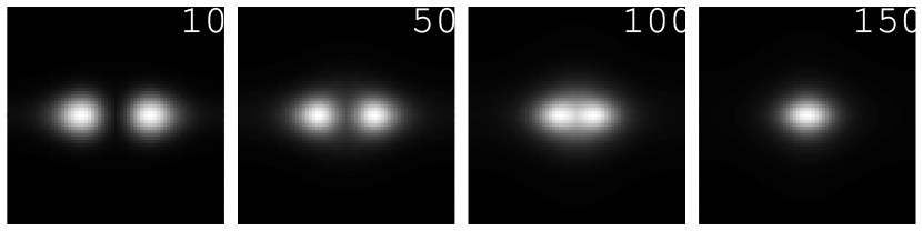
Figure 2: Snapshots at times $X^{0}\,m_{R}=10$, $50$, $100$ and $150$ of the initially anisotropic occupation number distribution as a function of $p_{\perp}$ (vertical) and $p_{\parallel}$ (horizontal). Bright (dark) regions correspond to high (low) occupation numbers. The shown resolution was achieved by using a $64^{3}$ spatial lattice.

More precisely, we investigate a class of spatially homogeneous initial conditions parametrized as

$$F(x^{0},y^{0};{\vec{p}})|_{x^{0}=y^{0}=0}=\frac{n_{0}({\vec{p}})+1/2}{\omega_{p}}\,,$$ (4.30)

with $\partial_{x^{0}}F(x^{0},0;{\vec{p}})|_{x^{0}=0}=0$, $\partial_{x^{0}}\partial_{y^{0}}F(x^{0},y^{0};{\vec{p}})|_{x^{0}=y^{0}=0}=[n_{0}({\vec{p}})+1/2]\,\omega_{p}$ for $\omega_{p}\equiv\sqrt{p_{\perp}^{2}+p_{\parallel}^{2}+M_{0}^{2}}$ and $M^{2}_{0}\equiv M^{2}(x^{0}=0)$. The initial distribution function $n_{0}({\vec{p}})$ is peaked around the “tsunami” momentum $p_{ts}$ with amplitude $A$ and width $\sigma$:

$$n_{0}({\vec{p}})=A\,\exp\left\{-\frac{1}{2\sigma^{2}}\left[p_{\perp}^{2}+(|p_{\parallel}|-p_{\rm ts})^{2}\right]\right\}\,.$$ (4.31)

We compute the nonequilibrium dynamics for a rather weak coupling of the $g^{2}\Phi^{4}$–interaction. For Fig. 2 we use $g^{2}=0.25$ and an initial distribution peaked at $p_{\rm ts}=0.8\,m_{R}$ with $A=20$ and $\sigma=0.32\,m_{R}$. For these parameters we obtain $t_{\rm damp}\simeq 100/m_{R}$ according to Eq. (4.29). We will consider a range of different couplings and amplitudes below.

The question is whether transport or kinetic equations can be used to quantitatively describe the early-time behavior before $t_{\rm damp}$, which is necessary if their application to the problem of fast apparent thermalization explained in Sec. 1 is viable. This is discussed in the following comparing to LO or NLO transport equations.

4.1 Isotropization

Figure 3: The solid line shows the on-shell $\partial_{X^{0}}\Delta\tilde{F}$ in Wigner coordinates, as computed from the solution of Eqs. (2.5)–(2.6) without a gradient expansion. The dashed line represents the same quantity using the expression from the LO gradient expansion according to Eq. (3.24). If the gradient expansion to lowest order is correct, then both lines have to agree. For this quantity one observes that the lowest-order gradient expansion becomes valid on a time scale of about the isotropization or damping time $t_{\rm damp}\simeq 100/m_{R}$. The inset shows the same results on a logarithmic scale to make the small on-shell $\partial_{X^{0}}\Delta\tilde{\varrho}$ visible. Its full result is given by the solid lower line, whereas the LO contribution is zero.

A characteristic anisotropy measure can be chosen as [11]

$$\Delta\tilde{F}(X^{0};\omega,p_{\rm ts})\equiv\tilde{F}(X^{0};\omega,{\vec{p}})|_{p_{\perp}=0,p_{\parallel}=p_{\rm ts}}-\tilde{F}(X^{0};\omega,{\vec{p}})|_{p_{\perp}=p_{\rm ts},p_{\parallel}=0}\,,$$ (4.32)

which vanishes for the case of an isotropic correlator since the latter depends on ${\vec{p}}^{2}=p_{\perp}^{2}+p_{\parallel}^{2}$. Fig. 3 shows the time evolution of the on-shell derivative $\partial_{X^{0}}\Delta\tilde{F}(X^{0};\omega(p_{\rm ts}),p_{\rm ts})$ [11]. The thick curve represents the full result, which is obtained from solving the evolution equations (2.5) and (2.6) for the self-energies (2.9) and (2.10) without any gradient expansion. For comparison, we evaluate the same quantity using the LO gradient expansion according to Eq. (3.24). For this we evaluate the RHS of Eq. (3.24) using the full result for $\tilde{F}(X^{0};\omega,{\vec{p}})$ and $\tilde{\varrho}(X^{0};\omega,{\vec{p}})$. If the gradient expansion to lowest order is correct, then both results have to agree. Indeed, one observes from Fig. 3, employing the same parameters as for Fig. 2, that the curves for the LO (dashed) and the full result agree well at sufficiently late times. However, they only agree after some time, which is rather well determined by the characteristic time scale $\sim t_{\rm damp}$ for the effective loss of details about the initial conditions. The latter is given by the thermal equilibrium estimate (4.29). Similarly, one can observe this time scale from the decay of the unequal-time spectral function in thermal equilibrium, $\rho^{\rm(eq)}(t;{\vec{p}}_{\rm ts})$ as explained below. The latter measures the characteristic decay of correlations at time $t$ with the initial state. The decay time for $\rho^{\rm(eq)}$ coincides rather well with the time for the onset of validity of the LO result.

Figure 4: Same as in Fig. 3 but for amplitudes $A=2,3,4$, i.e. smaller occupation numbers according to Eq. (4.31), and coupling $g^{2}=0.5$. The lower solid/dashed/dotted curves represent the full result, while the upper (thick) ones show the respective LO approximation.

Using smaller amplitudes $A$ (with $\sigma$ and $p_{\rm ts}$ kept fixed) one observes a similar picture. In Fig. 4 we compare runs for $A=2$, $3$ and $4$ with $g^{2}=0.5$. For instance, for $A=3$ the LO order and the full result approach each other rather closely after a time of about $500/m_{R}$. This time is rather well described by the characteristic decay time of the unequal-time correlator $\rho^{\rm(eq)}$ as shown in the inset of Fig. 5. Of course, the precise notion of a time after which a transport description holds depends on the definition and prescribed accuracy. We find for $A=2,3,4$ that the damping time according to Eq. (4.29) is $t_{\rm damp}=270,183,141m_{R}^{-1}$. For $A=3$ this time may be compared to the inset of Fig. 5, which shows that only after, say, a time of about $500m_{R}^{-1}$ the correlator is small enough that initial-time effects play no important role.

Figure 5: Comparison of LO, NLO and full result for the on-shell $\partial_{X^{0}}\Delta\tilde{F}$ with $A=3$ and $g^{2}=0.5$. For this quantity LO and NLO results do not differ much, while there is a substantial deviation from the full result at early times. The inset displays the real-time equilibrium spectral function for the considered mode, which exhibits the characteristic damping time for (partial) memory loss. The latter agrees rather well with the time for the onset of validity of a transport description.

One may expect that the failure of the LO transport equations to describe the dynamics before isotropization completes is due to substantial NLO contributions. However, this turns out not to be the case. Fig. 5 compares LO, NLO and full result for the time evolution of the on-shell $\partial_{X^{0}}\Delta\tilde{F}(X^{0};\omega(p_{\rm ts}),p_{\rm ts})$ for $A=3$ and $g^{2}=0.5$. The solid line represents the result as computed from the solution of Eq. (2.5) without a gradient expansion. As before, the dashed line shows the same quantity according to the LO expression given by the RHS of Eq. (3.24) using the full results $\tilde{F}(X^{0};\omega,{\vec{p}})$ and $\tilde{\varrho}(X^{0};\omega,{\vec{p}})$. Similarly, we evaluate the RHS of the NLO expression given by the RHS of Eq. (3.26). The result corresponds to the dotted line in Fig. 5, which turns out to be rather close to the LO curve.

For the quantity $\partial_{X^{0}}\Delta\tilde{F}(X^{0};\omega(p_{\rm ts}),p_{\rm ts})$ the NLO corrections remain small even for rather strong couplings. This is demonstrated in Fig. 6 for $g^{2}=1$ and same initial conditions as for Fig. 5. The convergence of the gradient expansion itself is apparently quite good here even for couplings of order one. However, when studying the importance of NLO corrections one has to distinguish between quantities whose vanishing corresponds to an enhanced symmetry from more generic quantities. Once an ensemble is isotropic it always remains so at later times even though the dynamics may still be far from equilibrium. The vanishing of $\Delta\tilde{F}$ obviously corresponds to an enhanced symmetry, i.e. rotation symmetry. In the following we consider more generic cases.

Figure 6: Same as in Fig. 5 but for $g^{2}=1$. Even for this stronger coupling the NLO corrections remain small, while there is a substantial deviation from the full result at early times.

4.2 Thermal equilibration

It has been demonstrated in Ref. [11] that in a scalar theory isotropization happens much faster than the approach to thermal equilibrium. Only a subclass of those processes that lead to thermalization are actually required for isotropization: “ordinary” $2\leftrightarrow 2$ scattering processes are sufficient in order to isotropize a system, while global particle number changing processes are crucial to approach thermal equilibrium.

Above we have investigated a quantity measuring an anisotropy ($\partial_{X^{0}}\Delta\tilde{F}$), and which, therefore, approaches zero rather quickly after $t_{\rm damp}$. Consequently, it is not affected by the relevant late-time processes which finally lead to a Bose-Einstein distribution. The accuracy of the gradient expansion for the late-time behavior can be investigated considering $\partial_{X^{0}}\tilde{F}(X^{0};\omega,{\vec{p}})$ instead, which does not vanish for an isotropic ensemble. Fig. 7 shows the time evolution for this quantity on shell at zero momentum for the same parameters as for Fig. 5. The solid lines give the full result for $\partial_{X^{0}}\tilde{F}$ (upper curve) and for $\partial_{X^{0}}\tilde{\varrho}$ (lower curve). This is compared to the LO (dashed) and NLO (dotted) results evaluated in the same way as explained above.

Figure 7: Comparison of LO, NLO and full result for the on-shell $\partial_{X^{0}}\tilde{F}$ at zero momentum with $A=3$ and $g^{2}=0.5$. The lower curves show the full and NLO result for $\partial_{X^{0}}\tilde{\varrho}$, to lowest order there is no contribution. The LO transport equation fails to describe the full results until rather late times. In contrast, taking into account the substantial NLO corrections the gradient expansion becomes quite accurate for times larger than about the characteristic damping time for partial memory loss.

One observes from Fig. 7 that the LO and the full result approach each other only at a time much later than it happens for the anisotropy quantity $\Delta\tilde{F}$ discussed in Sec. 4.1. However, one also observes from Fig. 7 that here the NLO corrections are substantial. The NLO results are much closer to the full result for times larger than about $\sim t_{\rm damp}$. We emphasize that the employed coupling $g^{2}=0.5$ is not very large. The situation is qualitatively not very different also for couplings of order one, which is exemplified in Fig. 8 for the same parameters as for Fig. 6. One observes, however, that the deviations of the NLO from the full result are stronger even at rather late times in this case.

Figure 8: Same as in Fig. 7 but for $g^{2}=1$.

We conclude that quantities which are sensitive to the late-time dynamics can receive important corrections at NLO in the gradient expansion. This finding is, of course, not surprising for strong couplings. However, sizeable NLO corrections can be obtained already for couplings of about $g^{2}\simeq 1/4$. Nevertheless, we observe that for not too early times the NLO result can get rather close to the full result for $g^{2}\lesssim 1$. The agreement of the (NLO) transport description and full results start at about the same time as for the isotropization case discussed above. Times shorter than about $t_{\rm damp}$ are clearly beyond the range of validity of transport equations even for weak couplings. This limitation is apparently not a consequence of a gradient expansion to low orders. The latter seems to converge rather well for weak enough couplings.

The failure of transport equations to describe early-time dynamics seems mainly based on the fact that the underlying assumptions 1) and 3) of Sec. 3.1 are not controlled by a small parameter. The validity of the standard assumptions 1) and 3) both require an efficient loss of correlations with the initial state. The characteristic time scale for this loss is given by the inverse damping rate of the unequal-time correlator $\rho^{(eq)}(t,{\vec{p}})$ or, similarly, by $\langle\Phi(t,{\vec{x}})\Phi(0,{\vec{y}})\rangle$. The latter describes the correlations with the initial time $t_{0}=0$. A vanishing $\langle\Phi(t,{\vec{x}})\Phi(0,{\vec{y}})\rangle$ corresponds to an effective loss of information about details of the initial conditions. The characteristic time scale for this loss is well described by $t_{\rm damp}$ as defined in Eq. (4.29) [11].

5 Off-shell transport

The gradient expansion underlying transport equations is an expansion in the number of derivatives with respect to the center coordinates (3.15) and derivatives with respect to momenta associated to the relative coordinates (3.16). The LO equations are obtained by neglecting ${\cal O}\left(\partial_{X^{\mu}}\partial_{p_{\mu}}\right)$ and higher contributions in the gradient expansion, the NLO equations by neglecting ${\cal O}\left(\left(\partial_{X^{\mu}}\partial_{p_{\mu}}\right)^{2}\right)$ etc. as described in Sec. 3. This expansion is constructed to work well for on-shell quantities, which are evaluated at the peak of the spectral function $\tilde{\varrho}(X^{0};\omega,{\vec{p}})$ as a function of $\omega$ for given ${\vec{p}}$. Away from this peak the contributions coming from derivatives with respect to momenta are typically not small if the spectral function is sufficiently narrow. The latter is always the case for weak enough couplings. Therefore, one may expect transport equations to fail for off-shell quantities even for weak couplings.

In order to quantify this expectation, we have in mind a nonequilibrium situation for a given time $X^{0}$ larger than $\sim t_{\rm damp}$ but short compared to characteristic thermal equilibration times. In this case the occupation number can still show substantial deviations from a thermal distribution though certain properties, such as a fluctuation-dissipation relation

$$\tilde{F}(\omega,{\vec{p}})=\left(n(\omega)+\frac{1}{2}\right)\tilde{\varrho}(\omega,{\vec{p}})\,,$$ (5.33)

with a non-thermal distribution $n(\omega)$, can become approximately valid [27]. We assume that the spectral function may be approximated by its equilibrium form

$$\tilde{\varrho}(\omega,{\vec{p}})=\frac{-\tilde{\Sigma}_{\varrho}(\omega,{\vec{p}})}{\left(-\omega^{2}+{{\vec{p}}}^{2}+M^{2}+\frac{1}{2}\tilde{\Sigma}_{+}(\omega,{\vec{p}})\right)^{2}+\left(\frac{1}{2}\tilde{\Sigma}_{\varrho}(\omega,{\vec{p}})\right)^{2}}\,,$$ (5.34)

while the non-thermal distribution will be parameterized as (cf. also Eq. (4.31))

$$n(\omega)=A\exp\left\{-\frac{1}{2\sigma^{2}}(\omega-\omega_{0})^{2}\right\}\,.$$ (5.35)

We employ Eq. (5.33) with Eqs. (5.34) and (5.35) as a convenient class of approximate parametrizations of typical nonequilibrium situations at intermediate times as have been studied in the previous sections. With the self-energies (2.9) and (2.10) in Fourier-space (cf. Sec. 3.1) these form a closed set of self-consistent equations for $\tilde{F}(\omega,{\vec{p}})$ and $\tilde{\varrho}(\omega,{\vec{p}})$.

Figure 9: The different curves of each graph show the different contributions $\tilde{F}\tilde{\Sigma}_{\varrho}-\tilde{\varrho}\tilde{\Sigma}_{F}$ (solid line), $\partial_{X^{0}}M^{2}\partial_{\omega}\tilde{F}$ (dashed) and $\frac{1}{2}\{\tilde{\Sigma}_{F},\tilde{\varrho}_{+}\}_{PB}+\frac{1}{2}\{\tilde{\Sigma}_{+},\tilde{F}\}_{PB}$ (dotted). The first corresponds to the LO contribution in the gradient expansion, while the latter two add up to the NLO contribution.

From these solutions we evaluate the LO and NLO expressions for $\partial_{X^{0}}\tilde{F}\left(X^{0};\omega,{\vec{p}}\right)$ according to Eqs. (3.24) and (3.26) in the very same way as described in Sec. 4. The results are shown in Fig. 9 for various couplings as a function of $(\omega-m_{R})/\gamma$ for ${\vec{p}}=0$ with $A=1$ and $\sigma=m_{R}$. Here $\gamma$ corresponds to the half width of the spectral function. The different curves of each graph show the different contributions $[\tilde{F}\tilde{\Sigma}_{\varrho}-\tilde{\varrho}\tilde{\Sigma}_{F}]/2\omega$ (solid line), $\partial_{X^{0}}M^{2}\partial_{\omega}\tilde{F}/2\omega$ (dotted) and $\left[\{\tilde{\Sigma}_{F},\tilde{\varrho}_{+}\}_{PB}+\{\tilde{\Sigma}_{+},\tilde{F}\}_{PB}\right]/4\omega$ (dashed) to the transport equation (3.26). The first corresponds to the LO contribution in the gradient expansion, while the latter two add up to the NLO contribution. One observes that the LO contribution has its maximum value on shell, i.e. for $\omega=m_{R}$. For small enough couplings we clearly find that the on-shell NLO corrections are small compared to LO ones.

In contrast, Fig. 9 shows that for small couplings the NLO corrections have their maximum contributions off shell. They easily exceed the LO terms away from $\omega\simeq m_{R}$ and here a gradient expansion to low orders cannot be expected to converge well. When the coupling grows to about $g^{2}\simeq 1/4$ the situation changes qualitatively. Here the Poisson-brackets contribution at NLO becomes comparable to the LO terms on shell. Though one expects transport equations to become unreliable for sufficiently large couplings, one observes for our example that NLO starts to become comparable to LO already for rather weak interactions. We emphasize that the normalization $g^{2}\Phi^{4}$ we use to define our coupling reflects rather well the separation between a weakly ($g^{2}\ll 1$) and strongly coupled regime ($g^{2}\gg 1$). To see this we consider the ratio between damping rate and oscillation frequency of the unequal-time correlator $\rho(t,{\vec{p}})$, which we denote as $2\pi\gamma/\omega$. Here $2\pi\gamma/\omega\ll 1$ corresponds to very weakly damped oscillations, while $2\pi\gamma/\omega\gg 1$ is overdamped. For comparison we display the corresponding values for this ratio in Fig. 9. One observes that they reflect rather well the coupling strength for the range of couplings considered here.

6 Conclusions

For the considered scalar $g^{2}\Phi^{4}$ theory we find that the earliest time for the validity of transport equations is well characterized by the standard relaxation or damping time $t_{\rm damp}$ given by Eq. (4.29). We have done a series of comparisons for various couplings and conclude that for times sufficiently large compared to $t_{\rm damp}$ the gradient expansion seems to converge well. There are sizeable NLO corrections already for couplings of about $g^{2}\simeq 1/4$. Nevertheless, one observes that the NLO result can get rather close to the “full” result for $g^{2}\lesssim 1$. Times shorter than about $t_{\rm damp}$ seem clearly beyond the range of validity of transport equations even for weak couplings. This should make them unsuitable to discuss aspects of apparent early thermalization and stresses the need to employ proper equations such as (2.5) and (2.6) for initial-value problems.

References

- [1] U. W. Heinz, “Thermalization at RHIC,” AIP Conf. Proc. 739 (2005) 163 [arXiv:nucl-th/0407067].
- [2] J. Berges, “Introduction to nonequilibrium quantum field theory,” AIP Conf. Proc. 739 (2005) 3 [arXiv:hep-ph/0409233].
- [3] J. Berges and J. Cox, “Thermalization of quantum fields from time-reversal invariant evolution equations,” Phys. Lett. B 517 (2001) 369 [arXiv:hep-ph/0006160].
- [4] J. Berges, “Controlled nonperturbative dynamics of quantum fields out of equilibrium,” Nucl. Phys. A 699 (2002) 847 [arXiv:hep-ph/0105311].
- [5] F. Cooper, J. F. Dawson and B. Mihaila, “Quantum dynamics of phase transitions in broken symmetry lambda phi4 field theory,” Phys. Rev. D 67 (2003) 056003 [arXiv:hep-ph/0209051].
- [6] J. Berges, S. Borsanyi and J. Serreau, “Thermalization of fermionic quantum fields,” Nucl. Phys. B 660 (2003) 51 [arXiv:hep-ph/0212404].
- [7] S. Juchem, W. Cassing and C. Greiner, “Quantum dynamics and thermalization for out-of-equilibrium phi4-theory,” Phys. Rev. D 69 (2004) 025006 [arXiv:hep-ph/0307353].
- [8] A. Arrizabalaga, J. Smit and A. Tranberg, “Equilibration in phi**4 theory in 3+1 dimensions,” Phys. Rev. D 72 (2005) 025014 [arXiv:hep-ph/0503287].
- [9] J. M. Cornwall, R. Jackiw and E. Tomboulis, “Effective Action For Composite Operators,” Phys. Rev. D 10 (1974) 2428; see also J. M. Luttinger and J. C. Ward, Phys. Rev. 118 (1960) 1417; G. Baym, Phys. Rev. 127 (1962) 1391.
- [10] G. Aarts, D. Ahrensmeier, R. Baier, J. Berges and J. Serreau, “Far-from-equilibrium dynamics with broken symmetries from the 2PI-1/N expansion,” Phys. Rev. D 66 (2002) 045008 [arXiv:hep-ph/0201308].
- [11] J. Berges, S. Borsanyi and C. Wetterich, “Isotropization far from equilibrium,” Nucl. Phys. B to appear [arXiv:hep-ph/0505182].
- [12] J. Berges, “n-Particle irreducible effective action techniques for gauge theories,” Phys. Rev. D 70 (2004) 105010 [arXiv:hep-ph/0401172].
- [13] R.E. Norton and J.M. Cornwall, Ann. Phys. (N.Y.) 91 (1975) 106. H. Kleinert, Fortschritte der Physik 30 (1982) 187. A.N. Vasiliev, Functional Methods in Quantum Field Theory and Statistical Physics, Gordon and Breach Science Pub. (1998); cf. also C. De Dominicis and P. C. Martin, J. Math. Phys. 5 (1964) 14, 31.
- [14] L. Kadanoff and G. Baym, “Quantum Statistical Mechanics”, Benjamin, New York, 1962.
- [15] P. Danielewicz, “Quantum Theory Of Nonequilibrium Processes. I,” Annals Phys. 152 (1984) 239. S. Mrowczynski and P. Danielewicz, “Green Function Approach To Transport Theory Of Scalar Fields,” Nucl. Phys. B 342, 345 (1990). S. Mrowczynski and U. W. Heinz, “Towards a relativistic transport theory of nuclear matter,” Annals Phys. 229 (1994) 1.
- [16] E. Calzetta and B. L. Hu, “Nonequilibrium Quantum Fields: Closed Time Path Effective Action, Wigner Function And Boltzmann Equation,” Phys. Rev. D 37, 2878 (1988).
- [17] D. Boyanovsky, I. D. Lawrie and D. S. Lee, “Relaxation and Kinetics in Scalar Field Theories,” Phys. Rev. D 54 (1996) 4013 [arXiv:hep-ph/9603217].
- [18] S. M. H. Wong, “Thermal and chemical equilibration in a gluon plasma,” Nucl. Phys. A 607 (1996) 442 [arXiv:hep-ph/9606305];
- [19] Y. B. Ivanov, J. Knoll and D. N. Voskresensky, “Self-consistent approximations to non-equilibrium many-body theory,” Nucl. Phys. A 657 (1999) 413 [arXiv:hep-ph/9807351]. J. Knoll, Y. B. Ivanov and D. N. Voskresensky, “Exact Conservation Laws of the Gradient Expanded Kadanoff-Baym Equations,” Annals Phys. 293 (2001) 126 [arXiv:nucl-th/0102044].
- [20] P. Lipavsky, K. Morawetz and V. Spicka, “Kinetic equation for strongly interacting dense Fermi systems,” Annales de Physique, Vol. 26, No. 1 (2001) 1.
- [21] S. Leupold, “Towards a test particle description of transport processes for states with continuous mass spectra,” Nucl. Phys. A 672 (2000) 475 [arXiv:nucl-th/9909080].
- [22] J. P. Blaizot and E. Iancu, “The quark-gluon plasma: Collective dynamics and hard thermal loops,” Phys. Rept. 359, 355 (2002) [arXiv:hep-ph/0101103].
- [23] A. Jakovac, “Generalized Boltzmann equations for on-shell particle production in a hot plasma,” Phys. Rev. D 66 (2002) 125003 [arXiv:hep-ph/0207085].
- [24] J. Berges and M. M. Muller, “Nonequilibrium quantum fields with large fluctuations,” in Progress in Nonequilibrium Green’s Functions II, eds. M. Bonitz and D. Semkat, World Scientific (2003) [http://arXiv:hep-ph/0209026].
- [25] T. Prokopec, M. G. Schmidt and S. Weinstock, “Transport equations for chiral fermions to order h-bar and electroweak baryogenesis,” Annals Phys. 314 (2004) 208 [arXiv:hep-ph/0312110]. Annals Phys. 314 (2004) 267 [arXiv:hep-ph/0406140].
- [26] T. Ikeda, “The effect of memory on relaxation in a scalar field theory,” Phys. Rev. D 69 (2004) 105018 [arXiv:hep-ph/0401045].
- [27] S. Borsanyi, “Thermal features far from equilibrium: prethermalization”, in SEWM02, ed. M.G. Schmidt (World Scientific, 2003) [arXiv:hep-ph/0409184].