Fermion Delocalization in Higgsless Models

Abstract:

In the linear moose framework, which naturally emerges in deconstruction models, we discuss the effect of direct couplings between the left-handed fermions living on the boundary of the chain and the gauge fields in the internal sites. This is realized by means of a product of nonlinear sigma-model scalar fields which, in the continuum limit, is equivalent to a Wilson line. The effect of these new nonlocal couplings is a contribution to the S parameter which can be of opposite sign with respect to the one coming from the gauge fields along the string. Therefore, with some fine-tuning, it is possible to satisfy the constraints from the electro-weak data without spoiling the perturbative unitarity limit, which, in these models is generally postponed with respect to the Higgsless Standard Model one.

1 Higgsless electro-weak symmetry breaking from moose models

Higgsless models may represent an alternative to the standard electro-weak (EW) symmetry breaking mechanism. In the past few years, after the blooming of extra-dimensions, they have received a renewal of interest. Higgsless models, in their ”modern” version, are formulated as gauge theories in a five dimensional space and, after decompactification, describe a tower of Kaluza Klein (KK) excitations of the standard EW gauge bosons [1]. One of the interesting features of these schemes is the possibility to delay the unitarity violation scale via the exchange of massive KK modes [1]. However, it is generally difficult to reconcile a delayed unitarity with the EW constraints. For instance in the framework of models with only ordinary fermions, it is possible to get a small or zero $S$ parameter [2], at the expenses of having a unitarity bound as in the Standard Model (SM) without the Higgs, that is of the order of 1 TeV. A recent solution to the problem which does not spoil the unitarity requirement at low scales, has been found by delocalizing the fermions in five dimensional theories [3, 4]. We will investigate this possibility in the context of deconstructed gauge theories which come out when the extra dimension is discretized [5]. Through discretization of the fifth dimension we get a finite set of four-dimensional gauge theories each of them acting at a particular lattice site. In this construction, any connection field along the fifth dimension, $A_{5}$, goes naturally into the link variables $\Sigma_{i}=e^{-iaA_{5}^{i-1}}$ realizing the parallel transport between two lattice sites (here $a$ is the lattice spacing). They satisfy the condition $\Sigma\Sigma^{\dagger}=1$ and can be identified with chiral fields. In this way the discretized version of the original 5-dimensional gauge theory is substituted by a collection of four-dimensional gauge theories with gauge interacting chiral fields $\Sigma_{i}$, synthetically described by a moose diagram (an example is given in Fig. 1).

Here we will consider the simplest linear moose model for the Higgsless breaking of the EW symmetry and we will delocalize fermions by introducing direct couplings between ordinary left-handed fermions and the gauge vector bosons along the moose string [6].

Let us briefly review the linear moose model based on the $SU(2)$ symmetry [2, 6]. We consider $K+1$ non linear $\sigma$-model scalar fields $\Sigma_{i}$, ${i=1,\cdots,K+1}$, $K$ gauge groups, $G_{i}$, ${i=1,\cdots,K}$ and a global symmetry $G_{L}\otimes G_{R}$ as shown in Fig. 1.

Figure 1: The simplest moose diagram for the Higgsless breaking of the EW symmetry.

A minimal model of EW symmetry breaking is obtained by choosing $G_{i}=SU(2)$, $G_{L}\otimes G_{R}=SU(2)_{L}\otimes SU(2)_{R}$. The SM gauge group $SU(2)_{L}\times U(1)_{Y}$ is obtained by gauging a subgroup of $G_{L}\otimes G_{R}$. The $\Sigma_{i}$ fields can be parameterized as $\Sigma_{i}=\exp{[i/(2f_{i})\vec{\pi}_{i}\cdot\vec{\tau}}]$ where $\vec{\tau}$ are the Pauli matrices and $f_{i}$ are $K+1$ constants that we will call link couplings. The lagrangian of the linear moose model is given by

$${\cal L}=\sum_{i=1}^{K+1}f_{i}^{2}{\rm Tr}[D_{\mu}\Sigma_{i}^{\dagger}D^{\mu}\Sigma_{i}]-\frac{1}{2}\sum_{i=1}^{K}{\rm Tr}[(F_{\mu\nu}^{i})^{2}]-\frac{1}{2}{\rm Tr}[(F_{\mu\nu}(\tilde{{W}}))^{2}-\frac{1}{2}{\rm Tr}[(F_{\mu\nu}(\tilde{{Y}}))^{2}],$$ (1)

with the covariant derivatives defined as follows: $D_{\mu}\Sigma_{1}=\partial_{\mu}\Sigma_{1}-i\tilde{g}\tilde{{W}}_{\mu}\Sigma_{1}+i\Sigma_{1}g_{1}V_{\mu}^{1}$; $~{}D_{\mu}\Sigma_{i}=\partial_{\mu}\Sigma_{i}-ig_{i-1}V_{\mu}^{i-1}\Sigma_{i}+i\Sigma_{i}g_{i}V_{\mu}^{i}~{}~{}(i=2,\cdots,K)$; $~{}D_{\mu}\Sigma_{K+1}=\partial_{\mu}\Sigma_{K+1}-ig_{K}V_{\mu}^{K}\Sigma_{K+1}+i\tilde{g}^{\prime}\Sigma_{K+1}\tilde{{Y}}_{\mu}$, where $V_{\mu}^{i}=V_{\mu}^{ia}\tau^{a}/2$ and $g_{i}$ are the gauge fields and gauge coupling constants associated to the groups $G_{i}$, $i=1,\cdots,K$, and $\tilde{{W}}_{\mu}=\tilde{{W}}_{\mu}^{a}\tau^{a}/2$, $\tilde{{Y}}_{\mu}={\tilde{\cal Y}}_{\mu}\tau^{3}/2$ are the gauge fields associated to $SU(2)_{L}$ and $U(1)_{Y}$ respectively. Notice that, in the unitary gauge, all the $\Sigma_{i}$ fields are eaten up by the gauge bosons which acquire mass, except for the photon corresponding to the unbroken $U(1)_{em}$. By identifying the lowest mass eigenvalue in the charged sector at $O(\tilde{g}^{2}/g_{i}^{2})$ with $M_{W}$, we get a relation between the EW scale v ($\approx 250~{}GeV$) and the link couplings of the chain:

$$\frac{4}{{\rm v}^{2}}\equiv\frac{1}{f^{2}}=\sum_{i=1}^{K+1}\frac{1}{f_{i}^{2}}.$$

Concerning fermions, we will consider only the standard model ones, that is: left-handed fermions $\psi_{L}$ as $SU(2)_{L}$ doublets and singlet right-handed fermions $\psi_{R}$ coupled to the SM gauge fields through the groups $SU(2)_{L}$ and $U(1)_{Y}$ at the ends of the chain.

2 Constraints from perturbative unitarity and EW tests

The worst high-energy behavior of the moose models arises from the scattering of longitudinal vector bosons. To simplify the calculation we will make use of the equivalence theorem, that is of the possibility of evaluating this amplitude in terms of the scattering amplitude of the corresponding Goldstone bosons. However this theorem holds in the approximation where the energy of the process is much higher than the mass of the vector bosons. Let us evaluate the amplitude for the SM $W$ and $Z$ at energies $M_{W/Z}\ll E\ll M_{V_{i}}$. The unitary gauge for the $V_{i}$ bosons is given by the choice $\Sigma_{i}=\exp[if\vec{\pi}\cdot\vec{\tau}/(2f_{i}^{2})]$ with $f$ given in eq. (1) and $\vec{\pi}$ the GB’s giving mass to $W$ and $Z$. The resulting four-pion amplitude is

$$A_{\pi^{+}\pi^{-}\to\pi^{+}\pi^{-}}=-\frac{f^{4}u}{4}\sum_{i=1}^{K+1}\frac{1}{f_{i}^{6}}+\frac{f^{4}}{4}\sum_{i,j=1}^{K}L_{ij}\left((u-t)(s-M_{2})_{ij}^{-1}+(u-s)(t-M_{2})_{ij}^{-1}\right),$$ (2)

with $(M_{2})_{ij}$ the square mass matrix for the gauge fields, and $L_{ij}=g_{i}g_{j}(f_{i}^{-2}+f_{i+1}^{-2})(f_{j}^{-2}+f_{j+1}^{-2})$. In the high-energy limit, where we can neglect the second term in eq. (2), the amplitude has a minimum for all the $f_{i}$’s being equal to a common value $f_{c}$. As a consequence, the scale at which unitarity is violated by this single channel contribution is delayed by a factor $(K+1)$ with respect to the one in the SM without the Higgs: $\Lambda_{moose}=(K+1)\Lambda_{HSM}$.

However the moose model has many other longitudinal vector bosons with bad behaving scattering amplitudes. For energies much higher than all the masses of the vector bosons, we can determine the unitarity bounds by considering the eigenchannel amplitudes corresponding to all the possible four-longitudinal vector bosons. Since the unitary gauge for all the vector bosons is given by $\Sigma_{i}=\exp[i\vec{\pi}\cdot\vec{\tau}/(2f_{i})]$, the amplitudes are already diagonal, and the high-energy result is simply $A_{\pi_{i}\pi_{i}\to\pi_{i}\pi_{i}}\to-{u}/(4f_{i}^{2})$. We see that, also in this case, the best unitarity limit is for all the link couplings being equal: $f_{i}=f_{c}$. Then: $\Lambda^{TOT}_{moose}=\sqrt{K+1}~{}\Lambda_{HSM}$ (for similar results see ref. [23] in [6]). However, in order our approximation to be correct, we have to require $M_{V_{i}}^{max}\ll\Lambda^{TOT}_{moose}$. By using the explicit expression for the highest mass eigenvalue, in the case of equal couplings $g_{i}=g_{c}$, we get an upper bound $g_{c}<5$. As we will see, this choice gives unacceptable large EW correction.

In this class of models all the corrections from new physics are ”oblique” since they arise from mixing of the SM vector bosons with the moose vector fields (we are assuming the standard couplings for the fermions to $SU(2)_{L}\otimes U(1)$). As well known, the oblique corrections are completely captured by the parameters $S$, $T$ and $U$ or, equivalently by the parameters $\epsilon_{i}$, $i=1,2,3$. For the linear moose, the existence of the custodial symmetry $SU(2)_{V}$ ensures that $\epsilon_{1}\approx\epsilon_{2}\approx 0$. On the contrary, the new physics contribution to the EW parameter $\epsilon_{3}$ is sizeable and positive [2]: $\epsilon_{3}=(\tilde{g}^{2}/g_{i}^{2})\sum_{i=1}^{K}(1-y_{i})y_{i}$, where $y_{i}=\sum_{j=1}^{i}f^{2}/f_{j}^{2}$. Since $0\leq y_{i}\leq 1$ it follows $\epsilon_{3}\geq 0$ (see also [7, 8, 9]). As an example, let us take equal couplings along the chain: $f_{i}=f_{c}$, $g_{i}=g_{c}$. Then $\epsilon_{3}=\tilde{g}^{2}~{}K(K+2)/(6~{}g_{c}^{2}(K+1))$, which grows with the number of sites of the moose. If we want to be compatible with the experimental data we need to get $\epsilon_{3}\approx 10^{-3}$. Already for $K=1$ this would require $g_{c}\geq 15.8\tilde{g}$, implying a strong interacting gauge theory in the moose sector and unitarity violation. Notice also that, insisting on a weak gauge theory would imply $g_{c}$ of the order of $\tilde{g}$, then the natural value of $\epsilon_{3}$ would be of the order $10^{-1}-10^{-2}$, incompatible with the experimental data.

3 Effects of fermion delocalization

A way to reconcile perturbative unitarity requirements with the EW bounds is to allow delocalized couplings of the SM fermions to the moose gauge fields and some amount of fine tuning [6]. In fact, by genaralizing the procedure in [10], the SM fermions can be coupled to any of the gauge fields at the lattice sites by means of a Wilson line. Define $\chi_{L}^{i}=\Sigma_{i}^{\dagger}\Sigma_{i-1}^{\dagger}\cdots\Sigma_{1}^{\dagger}\psi_{L}$, for $i=1,\cdots,K$. Since under a gauge transformation, $\chi_{L}^{i}\to U_{i}\chi_{L}^{i}$, with $U_{i}\in G_{i}$, at each site we can introduce a gauge invariant coupling given by

$$b_{i}\bar{\chi}_{L}^{i}\gamma^{\mu}\left(\partial_{\mu}+ig_{i}V_{\mu}^{i}+\frac{i}{2}{\tilde{g}}^{\prime}(B-L)\tilde{{Y}}_{\mu}\right)\chi_{L}^{i},$$ (3)

where $B(L)$ is the barion(lepton) number and $b_{i}$ are dimensionless parameters. The new fermion interactions give extra non-oblique contributions to the EW parameters. These are calculated in [6] by decoupling the $V_{\mu}^{i}$ fields and evaluating the corrections to the relevant physical quantities. To the first order in $b_{i}$ and to $O(\tilde{g}^{2}/g_{i}^{2})$, the $\epsilon_{i}$ parameters are modified as follows:

$$\epsilon_{1}\approx 0,~{}~{}~{}\epsilon_{2}\approx 0,~{}~{}~{}\epsilon_{3}\approx\sum_{i=1}^{K}y_{i}\left(\frac{g^{2}}{g_{i}^{2}}(1-y_{i})-b_{i}\right).$$ (4)

This final expression suggests that the introduction of the $b_{i}$ direct fermion couplings to $V_{i}$ can compensate for the contribution of the tower of gauge vectors to $\epsilon_{3}$. This would reconcile the Higgsless model with the EW precision measurements by fine-tuning the direct fermion couplings.

In the simplest model with all $f_{i}=const=f_{c}$, $g_{i}=const=g_{c}$ and $b_{i}=const=b_{c}$, as shown in the left panel of Fig. 2, the experimental bounds from the $\epsilon_{3}$ parameter can be satisfied by fine-tuning the direct fermion coupling $b_{c}$ along a strip in the plane $(Kb_{c},\sqrt{K}/g_{c})$ (we have chosen these parameters due to the scaling properties of $g_{c}$ and $b_{c}$ with $K$, see ref. [6] for details).

The expression for $\epsilon_{3}$ given in eq. (4) suggests also the possibility of a site-by-site cancellation, provided by: $b_{i}=\delta(g^{2}/g_{i}^{2})(1-y_{i})$. This choice, for small $b_{i}$, gives $\epsilon_{3}\approx 0$ for $\delta=1$. Assuming again $f_{i}=f_{c}$, $g_{i}=g_{c}$, the allowed region in the space $(\delta,\sqrt{K}/g_{c})$ is given on the right panel of Fig. 2.

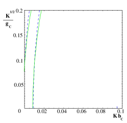
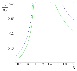
Figure 2: The 95% CL bounds on the plane $(Kb_{c},\sqrt{K}/g_{c})$-left panel, $(\delta,\sqrt{K}/g_{c})$-right panel, from the experimental value of $\epsilon_{3}$ for $K=1$ (solid green lines), $K=10$ (dash blue lines). The allowed regions are between the corresponding lines.

In conclusion, by fine tuning every direct fermion coupling at each site to compensate the corresponding contribution to $\epsilon_{3}$ from the moose gauge bosons (see also [11]), it is possible to satisfy the EW constraints and improve the unitarity bound of the Higgsless SM at the same time.

References

- [1] See references in [6].
- [2] R. Casalbuoni, S. De Curtis, and D. Dominici, Moose models with vanishing parameter, Phys. Rev. D70 (2004) 055010 [hep-ph/0405188].
- [3] G. Cacciapaglia, C. Csaki, C. Grojean, and J. Terning, Curing the ills of Higgsless models: The S parameter and unitarity, Phys. Rev. D71 (2005) 035015 [hep-ph/0409126].
- [4] R. Foadi, S. Gopalakrishna, and C. Schmidt, Effects of fermion localization in Higgsless theories and electroweak constraints, Phys. Lett. B606 (2005) 157 [hep-ph/0409266].
- [5] N. Arkani-Hamed, A. G. Cohen and H. Georgi, (De)constructing dimensions, Phys. Rev. Lett. 86 (2001) 4757 [hep-th/0104005], and references in [6].
- [6] R. Casalbuoni, S. De Curtis, D. Dolce and D. Dominici, Playing with fermion couplings in Higgsless models, Phys. Rev. D71 (2005) 075015 [hep-ph/0502209].
- [7] R. Barbieri, A. Pomarol and R. Rattazzi, Weakly coupled Higgsless theories and precision electroweak tests, Phys. Lett. B591, (2004) 141 [hep-ph/0310285].
- [8] J. Hirn and J. Stern, The role of spurions in Higgs-less electroweak effective theories, Eur. Phys. J. C34, (2004) 447 [hep-ph/0401032].
- [9] H. Georgi, Fun with Higgsless theories, Phys. Rev. D71, (2005) 015016 [hep-ph/0408067].
- [10] R. Casalbuoni, S. De Curtis, D. Dominici, and R. Gatto, Effective weak interaction theory with possible new vector resonance from a strong Higgs sector, Phys. Lett. B155 (1985) 95; and Physical implications of possible J = 1 bound states from strong Higgs, Nucl. Phys. B282 (1987) 235.
- [11] R. Sekhar Chivukula, E. H. Simmons, H. J. He, M. Kurachi and M. Tanabashi, Ideal fermion delocalization in Higgsless models, Phys. Rev. D72 (2005) 015008 [hep-ph/0504114]; and Ideal fermion delocalization in five dimensional gauge theories, Phys. Rev. D72 (2005) 095013 [hep-ph/0509110].