Realistic predictions are made for the rates of lepton flavour violating Higgs boson decays, $\tau\to\mu\gamma$, $\mu\to e\gamma$, $B_{s}^{0}\to\mu\mu$, $B_{s}^{0}\to\tau\mu$ and $\tau\to 3\mu$, via a top-down analysis of the Minimal Supersymmetric Standard Model(MSSM) constrained by $SU(5)$ unification with right-handed Neutrinos and large $\tan\beta$. The third family neutrino Yukawa coupling is chosen to be of order 1, in this way our model bares a significant resemblance to supersymmetric $SO(10)$. In this framework the large PMNS mixings result in potentially large lepton flavour violation. Our analysis predicts $\tau\to\mu\gamma$ and $\mu\to e\gamma$ rates in the region $(10^{-8}-10^{-6})$ and $(10^{-15}-10^{-14})$ respectively. We also show that the rates for lepton flavour violating Higgs decays can be as large as $10^{-7}$. The non-decoupling nature of $H^{0}\to\tau\mu$ is observed which leads to its decay rate becoming comparable to that for $\tau\to\mu\gamma$ for large values of $m_{0}$ and $M_{1/2}$. We also find that the present bound on $B_{s}\to\mu\mu$ is an important constraint on the rate of lepton flavour violating Higgs decays. The recently measured $B_{s}$-$\bar{B}_{s}$ mixing parameter $\Delta M_{s}$ is also investigated.

1 Introduction

Over the past few years the phenomenon of neutrino oscillations and neutrino masses have been confirmed by observations made by the Super-Kamiokande[1], SNO[2], K2K[3] and KamLAND[4] experiments. At the present time the experimental determination of oscillation parameters has become increasingly accurate. The resulting measurements have indicated large, almost bimaximal mixing in the lepton sector, hence Neutrino mixing appears to be markedly different from that of the quark sector of the Standard Model(SM). A combined Global fit to the three-neutrino framework leads to the following 2$\sigma$ oscillation parameter fit[5],

$$\delta m^{2}_{12} = 7.92(1\pm 0.09)\times 10^{-5}\,{\rm eV^{2}}\,\,\,\,{\rm at\,\,\pm 2\sigma}$$ (1)

$$\sin^{2}\theta_{12} = 0.314(1^{+0.18}_{-0.15})\,\,\,\,{\rm at\,\,\pm 2\sigma}$$ (2)

$$\Delta m^{2}_{23} = 2.4(1^{+0.21}_{-0.26})\times 10^{-3}\,{\rm eV^{2}}\,\,\,\,{\rm at\,\,\pm 2\sigma}$$ (3)

$$\sin^{2}\theta_{23} = 0.44(1^{+0.41}_{-0.22})\,\,\,\,{\rm at\,\,\pm 2\sigma}$$ (4)

$$\sin^{2}\theta_{13} = 0.9^{+2.3}_{-0.9}\times 10^{-2}\,\,\,\,{\rm at\,\,\pm 2\sigma}.$$ (5)

Neutrino oscillations are the first example of physics beyond the Standard Model. In the Standard Model of particle physics the lepton number of each generation is a conserved quantity. The observation of neutrino masses also marks the first evidence for flavour violation in the lepton sector and gives the possibility of lepton flavour violation (LFV) among the charged leptons. In the supersymmetric seesaw model, flavour violation at the high energy scale may feed into the charged lepton sector via radiatively induced off-diagonal elements of the left-slepton scalar mass, $m_{\tilde{L}}^{2}$. Hence the large mixings observed in neutrino oscillations could result in large lepton flavour violating rates for such decays as $\tau\to\mu\gamma$, $\mu\to e\gamma$ and $\tau\to e\gamma$.

Supersymmetric theories contain a number of possible sources of lepton flavour violation. As a result, the bounds on rates of LFV are particularly restricting upon the SUSY parameter space. Even in the case of minimal supergravity(mSUGRA), where soft SUSY breaking masses and trilinear couplings are flavour diagonal at the GUT scale, the presence of right-handed neutrinos and the PMNS mixings are enough to radiatively induce large LFV rates. It is these LFV rates, induced by renormalisation group(RG) running that we wish to study in the present work.

The processes $l_{i}\to l_{j}\gamma$ represent the most stringent bounds on lepton flavour violating interactions. The present experimental bounds are as follows,

$${\rm BR}(\mu\to e\gamma) < 1.2\times 10^{-11}\,\,\,{\rm at\,\,90\%\,\,C.L.}\cite[cite]{[\@@bibref{}{Brooks:1999pu}{}{}]}$$ (6)

$${\rm BR}(\tau\to\mu\gamma) < 3.1\times 10^{-7}\,\,\,{\rm at\,\,90\%\,\,C.L.}\cite[cite]{[\@@bibref{}{Hayasaka:2005tc}{}{}]}$$ (7)

$${\rm BR}(\tau\to e\gamma) < 3.9\times 10^{-7}\,\,\,{\rm at\,\,90\%\,\,C.L.}\cite[cite]{[\@@bibref{}{Hayasaka:2005tc}{}{}]}.$$ (8)

In the near future these decays will be studied at the PSI-MEG experiment and at the B-factories, which will set bounds in the region of,

$${\rm BR}(\mu\to e\gamma) < 5\times 10^{-14}\,\,\,\cite[cite]{[\@@bibref{}{MEG}{}{}]}$$ (9)

$${\rm BR}(\tau\to\mu\gamma) < 10^{-8}\,\,\,\cite[cite]{[\@@bibref{}{Hayasaka:2005tc}{}{}]}$$ (10)

$${\rm BR}(\tau\to e\gamma) < 10^{-8}\,\,\,\cite[cite]{[\@@bibref{}{Hayasaka:2005tc}{}{}]}.$$ (11)

When studying lepton flavour violating decay rates it is important to ensure that the rates for these rare lepton decays don’t exceed the experimental bounds listed above. In order to make realistic predictions for LFV rates within a complete SUSY model, it is useful to require a good fit to electroweak data including, fermion masses and mixings, correct electroweak symmetry breaking and the correct rate for $b\to s\gamma$.

Recently a number of Higgs mediated lepton flavour violating processes have also become interesting. These include, $B_{d,s}^{0}\to\tau\mu$[9], $\tau\to\mu\mu\mu$[10], $\tau\to\mu\eta\cite[cite]{[\@@bibref{}{Sher:2002ew}{}{}]}$ and lepton flavour violating decays of neutral Higgs bosons[12]. In the region of parameter space for which the neutral Higgs boson masses are light, these Higgs mediated decays can possibly become very interesting. Enhancement by large $\tan\beta$ adds to the possibilities even further. When discussing such rare decays it is very important to take into account the experimental bounds from $l_{i}\to l_{j}\,\gamma$, only then can meaningful predictions for such decay rates be made. Theoretical studies of such decays with supersymmetric models have reported interesting predictions with rates as high as,

$${\rm BR}(B_{s}^{0}\to\tau\mu) \sim 4\times 10^{-9}\,\,\cite[cite]{[\@@bibref{}{Dedes:2002rh}{}{}]}$$ (12)

$${\rm BR}(\tau\to\mu\mu\mu) \sim 10^{-7}\,\,\cite[cite]{[\@@bibref{}{Babu:2002et}{}{}]}$$ (13)

$${\rm BR}(\tau\to\mu\eta) \sim 10\times{\rm BR}(\tau\to\mu\mu\mu)\,\,\cite[cite]{[\@@bibref{}{Sher:2002ew}{}{}]}$$ (14)

$${\rm BR}(\phi^{0}\to\tau\mu) \sim 10^{-4}\,\,\cite[cite]{[\@@bibref{}{LFVhiggs}{}{}]},$$ (15)

where $\phi^{0}$ represents the neutral MSSM Higgs bosons, $\phi^{0}=A^{0},\,H^{0},\,h^{0}$.

The most exciting example of Higgs mediated decays is that of $B^{0}_{s,d}\to\mu\mu$[13] in the MSSM. This decay is proportional to $\tan^{6}\beta$ and so is greatly enhanced by large values of $\tan\beta$. If the Higgs boson is very light then this rate could become very exciting. The present experimental bounds for these rare $B^{0}_{s,d}$ decays are the following,

$${\rm BR}(B_{s}\to\mu\mu)\, < \,0.8\times 10^{-7}\,\,\,{\rm at\,\,90\%\,\,C.L.}\,\,\cite[cite]{[\@@bibref{}{CDFnote}{}{}]}$$ (16)

$${\rm BR}(B_{d}\to\mu\mu) < 2.3\times 10^{-8}\,\,\,{\rm at\,\,90\%\,\,C.L.}\,\,\cite[cite]{[\@@bibref{}{CDFnote}{}{}]}.$$ (17)

Theoretically the ratio $V_{ts}/V_{td}\sim 10$ means that the $B_{s}$ decay is more restrictive than that of $B_{d}$. These decays are of particular interest as the Standard model contributions enter at the 1-loop level which makes this a good place to search for physics beyond the standard model. In supersymmetric models it is expected that the dominant contribution to $B_{s,d}\to\mu\mu$ could come from a penguin diagram mediated by Higgs bosons. In such a scenario the present bound on $B_{s}\to\mu\mu$ will constrain the Higgs masses and in turn constrain the decay rate for $\phi^{0}\to\tau\mu$.

We propose to study the rates of lepton flavour violating decays of $\tau$, $B_{s,d}^{0}$ and MSSM Higgs bosons in a supersymmetric model based on $SU(5)$ unification with seesaw neutrinos and large $\tan\beta$. The quark and charged lepton sectors of this theory are well constrained with 9 parameters determining 12 low-energy observables. On the other hand the neutrino sector has more parameters than experimental observables. Therefore we must attempt to use bounds on lepton flavour violating decays to further constrain the parameters of the neutrino sector. From this theory we hope to make general predictions for some of the interesting lepton flavour violating decays mentioned above and also to study their correlations. The recently measured $B_{s}$-$\bar{B}_{s}$ mixing parameter $\Delta M_{s}$ is also investigated.

The present work differs from previous studies of lepton flavour violating Higgs decays in that our work uses a top-down analysis of a Grand Unified SUSY model. Also we are studying lepton flavour violating Higgs decays in conjunction with Higgs mediated decays, such as $B_{s}\to\mu\mu$, for the first time. It is shown that the experimental bound on $B_{s}\to\mu\mu$ provides important information regarding the allowed rates for lepton flavour violating Higgs decays. It is also shown that the Higgs contribution to $\Delta M_{s}$ via the often neglected operator $(\bar{b}_{R}s_{L})(\bar{b}_{R}s_{L})$ may be comparable to the contribution from the operator $(\bar{b}_{R}s_{L})(\bar{b}_{L}s_{R})$.

The rest of the paper is arranged as follows. A basic introduction to the supersymmetric $SU(5)$ model studied in the present work is given in section 2. A discussion of the relevant flavour violating phenomenology analysed in this paper is given in section 3 with an outline of our numerical procedure in section 4. In section 5 we present our results and discuss their implications. Finally, section 6 concludes the present work.

2 Minimal Supersymmetric $SU(5)$ with right-handed neutrinos

In the present work we shall study the MSSM$+\nu_{R}$ constrained at the GUT scale by $SU(5)$ unification. Let us first outline the general features of this model and then proceed to give details of the simplifying assumptions made during this analysis. In Minimal $SU(5)$ the matter superfields of the MSSM are contained within the representations; ${\bf 10}=(Q,\,U^{c},\,E^{c})$, and ${\bf\bar{5}}=(L,\,D^{c})$. The inclusion of right-handed neutrinos into the theory requires a further singlet superfield, ${\bf 1}=(N^{c})$. In addition there are ${\bf 5}$ and ${\bf\bar{5}}$ Higgs representations, ${\bf H}$ and ${\bf\bar{H}}$. These Higgs representations contain the MSSM Higgs doublets $H_{u}$, $H_{d}$.

Using these matter superfields we can construct the Yukawa section of the superpotential as follows,

$$W_{Y}^{SU(5)}=\frac{1}{8}\,Y_{u}^{ij}\,{\bf 10}_{i}{\bf 10}_{j}{\bf H}+Y_{d}^{ij}\,{\bf 10}_{i}{\bf\bar{5}}_{j}{\bf\bar{H}}+Y_{\nu}^{ij}\,{\bf\bar{5}}_{i}{\bf 1}_{j}{\bf H}+\frac{1}{2}\,M_{R}^{ij}\,{\bf 1}_{i}{\bf 1}_{j}.$$ (18)

The first term of eq. (18) gives rise to a symmetric up-quark Yukawa coupling $Y_{u}$ and the second term provides both down-quark and charged lepton Yukawa couplings. As a result we have the GUT scale relation, $Y_{e}={Y_{d}}^{\rm T}$, hence there exists GUT scale $b-\tau$ unification.

The final two terms in the superpotential of eq. (18) are responsible for the neutrino Yukawa coupling, $Y_{\nu}$ and the right-handed neutrino Majorana mass, $M_{R}$. These final two terms combine to produce the light neutrino mass matrix via the type I seesaw mechanism,

$$m_{LL}=\,-v_{u}^{2}\,\,Y_{\nu}\,{M_{R}}^{-1}\,{Y_{\nu}}^{\rm T}.$$ (19)

Our next step is to rotate away the non-physical degrees of freedom. We begin by rotating the ${\bf 10}$ and ${\bf\bar{5}}$ representations such that $Y_{d}$ is diagonal. As a result the coupling $Y_{u}$ is solely responsible for the CKM mixings. Therefore, from eq. (18) we can see that $Y_{u}$ is diagonalised by rotating the ${\bf 10}$-dimensional representation by the CKM matrix. The lepton sector is more complicated due to the structure of the see-saw mass matrix in eq. 19. Rotating the singlet neutrino such that the combination, $Y_{\nu}^{\rm T}Y_{\nu}$, is diagonal we can write,

$$Y_{u} = V_{CKM}^{\rm T}\,Y_{u}^{\rm diag}\,V_{CKM}$$

$$Y_{d} = Y_{d}^{\rm diag}$$

$$Y_{\nu} = U\,Y_{\nu}^{\rm diag}$$ (20)

$$M_{R} = W\,M_{R}^{\rm diag}\,W^{\rm T}.$$

Here $U$ and $W$ both represent unitary rotations. In the case were, $W=1$, the mixing matrix $U$ is identified as the PMNS matrix. For simplicity we assume that $W=1$ and that all parameters are real.

In the neutrino sector we have 9 parameters at the GUT scale, but only 4 low-energy observables. The bound on the undetermined neutrino mixing angle, $\theta_{13}$, also constrains the GUT scale mixing to be small. As a result and for simplicity we shall assume $\theta_{13}(M_{\rm GUT})=0$ in our present study. Throughout the analysis we have made the assumption that both the neutrino Yukawa and Majorana matrices have a hierarchical form with $Y_{\nu_{3}}^{\rm diag}\sim 1$ and $M_{R_{3}}\sim 10^{14}$ GeV, as shown in eq. (21) and (22). We choose such a hierarchy in the neutrino Yukawa sector with one eye on $b-t-\tau$ Yukawa unification and $SO(10)$ with $\tan\beta\sim 50$.

$$Y_{\nu_{1}}^{\rm diag}<Y_{\nu_{2}}^{\rm diag}<Y_{\nu_{3}}^{\rm diag}\sim 1$$ (21)

$$M_{R_{1}}^{\rm diag}<M_{R_{2}}^{\rm diag}<M_{R_{3}}^{\rm diag}\sim 10^{14}\,\,{\rm GeV}$$ . (22)

This type of hierarchy naturally leads a light neutrino scale $\sim 0.1$ eV. It seems that we are still left with a great deal of freedom in the neutrino sector with four parameters at the GUT scale determining only two mass squared differences at the weak scale. It is worth noting that if we had studied $SO(10)$ unification then the additional symmetry would provide a relation between each of the fermionic Yukawa couplings and so the neutrino sector would then be more predictive. Here we study $SU(5)$ as it is the prototypical unified group and in many ways it is the minimal unified theory. In $SU(5)$ the freedom in the neutrino sector must be constrained by bounds on the rates of lepton flavour violating decays such as $\mu\to e\gamma$, $\tau\to\mu\gamma$ and $\tau\to e\gamma$. From eq. (20) the neutrino Yukawa coupling at the GUT scale, assuming bimaximal neutrino mixing and $\theta_{13}=0$, takes the form,

$$Y^{\rm GUT}_{\nu}\,\approx\,\left(\begin{array}[]{ccc}\frac{1}{\sqrt{2}}\,Y^{\rm diag}_{\nu_{1}}&\frac{1}{\sqrt{2}}\,Y^{\rm diag}_{\nu_{2}}&0\\ -\frac{1}{2}\,Y^{\rm diag}_{\nu_{1}}&\frac{1}{2}\,Y^{\rm diag}_{\nu_{2}}&\frac{1}{\sqrt{2}}\,Y^{\rm diag}_{\nu_{3}}\\ \frac{1}{2}\,Y^{\rm diag}_{\nu_{1}}&-\frac{1}{2}\,Y^{\rm diag}_{\nu_{2}}&\frac{1}{\sqrt{2}}\,Y^{\rm diag}_{\nu_{3}}\end{array}\right).$$ (23)

Eq. (23) shows that the size of the off-diagonal terms in the neutrino Yukawa matrix are determined by the diagonal elements, $Y^{\rm diag}_{\nu_{1}}$, $Y^{\rm diag}_{\nu_{2}}$ and $Y^{\rm diag}_{\nu_{3}}$. Such terms will induce off-diagonal elements in the slepton mass squared matrix with the approximate form,

$$(\Delta m_{\tilde{L}}^{2})_{ij}\sim-\frac{{\rm ln}(M_{\rm GUT}/M_{R})}{16\pi^{2}}(6m_{0}^{2}+2A_{0}^{2})(Y_{\nu}Y_{\nu}^{\rm T})_{ij},\,\,\,\,i\neq j.$$ (24)

Here $m_{0}$ and $A_{0}$ are the usual universal soft scalar mass and trilinear couplings commonly present in minimal supergravity models. Finally this leads to radiatively induced lepton flavour violation through Feynman diagrams with sleptons inside the loop [17]. Clearly eq. (24) tells us that it is the size of $Y^{\rm diag}_{\nu_{i}}$ that will affect the rates for $l_{i}\to l_{j}\gamma$. For example with, $Y_{\nu_{3}}>Y_{\nu_{2}}$, it will be $Y_{\nu_{3}}$ which contributes strongly to the rate of $\tau\to\mu\gamma$. Hence the bounds on $\mu\to e\gamma$, $\tau\to\mu\gamma$ and $\tau\to e\gamma$ will act as a constraint on the size of $Y^{\rm diag}_{\nu}$. During our study we have chosen a neutrino Yukawa hierarchy of the approximate form,

$$Y^{\rm diag}_{\nu_{1}}:Y^{\rm diag}_{\nu_{2}}:Y^{\rm diag}_{\nu_{3}}\,\,\approx\,\,\lambda^{6}:\lambda^{4}:1$$ (25)

where $\lambda=0.22$. This neutrino Yukawa hierarchy is similar to the hierarchy in the up-quark Yukawa coupling, which naturally arises in simple $SO(10)$ models [18]. With, $Y_{\nu_{3}}\sim 1$, it is possible that $\mu$-$\tau$ lepton flavour violating rates will be near their experimental limits. This allows us to analyse predictions for other LFV decays while the rates for $\tau\to\mu\gamma$ are at the maximally allowed levels from experiment. In this way our predictions will be optimistic while remaining realistic.

Let us now examine the soft SUSY breaking section of the Lagrangian. For minimal $SU(5)$ the relevant section of the soft supersymmetry breaking Lagrangian takes the following form,

$$-{\mathcal{L}}_{soft} = \frac{1}{2}{\bf{\tilde{10}}}_{i}\,(m_{10}^{2})_{ij}\,{\bf{\tilde{10}}}^{\dagger}_{j}+{\bf\tilde{\bar{5}}}_{i}^{\dagger}\,(m_{5}^{2})_{ij}\,{\bf\tilde{\bar{5}}}_{j}+{\bf\tilde{1}}_{i}\,(m_{N}^{2})_{ij}\,{\bf\tilde{1}}_{j}^{\dagger}+m_{H}^{2}\,{\bf h}^{\dagger}{\bf h}+m_{\bar{H}}^{2}\,{\bf\bar{h}}^{\dagger}{\bf\bar{h}}$$ (26)

$$+\frac{1}{8}\,{\bf{\tilde{10}}}_{i}\,(A_{u})_{ij}\,{\bf{\tilde{10}}}_{j}\,{\bf h}+{\bf\tilde{\bar{5}}}_{i}\,(A_{d})_{ij}\,{\bf{\tilde{10}}}_{j}\,{\bf\bar{h}}+{\bf\tilde{\bar{5}}}_{i}\,(A_{N})_{ij}\,{\bf\tilde{1}}_{j}\,{\bf h}+\frac{1}{2}M_{24}\,{\bf\tilde{24}}{\bf\tilde{24}}.$$

Here ${\bf{\tilde{10}}}$, ${\bf\tilde{\bar{5}}}$, ${\bf\tilde{1}}$, ${\bf h}$ and ${\bf\bar{h}}$ are the scalar components of the fields, ${\bf{{10}}}$, ${\bf{\bar{5}}}$, ${\bf{1}}$, ${\bf H}$ and ${\bf\bar{H}}$. The final term of eq.(26) is the soft mass for the $SU(5)$ gaugino ${\bf\tilde{24}}$, which is the scalar component of the gauge boson adjoint representation, ${\bf 24}$. Below the GUT scale the soft SUSY breaking terms of the effective theory are given by,

$$- {\mathcal{L}}_{soft}=$$

$${\bf\tilde{Q}}_{i}^{\dagger}(m_{Q}^{2})_{ij}{\bf\tilde{Q}}_{j}+{\bf\tilde{\bar{d}}}_{i}(m_{{D}}^{2})_{ij}{\bf\tilde{\bar{d}}}_{j}^{\dagger}+{\bf\tilde{\bar{u}}}_{i}(m_{{U}}^{2})_{ij}{\bf\tilde{\bar{u}}}_{j}^{\dagger}+{\bf\tilde{L}}_{i}^{\dagger}(m_{L}^{2})_{ij}{\bf\tilde{L}}_{j}+{\bf\tilde{\bar{e}}}_{i}(m_{{E}}^{2})_{ij}{\bf\tilde{\bar{e}}}_{j}^{\dagger}+{\bf\tilde{\bar{n}}}_{i}(m_{N}^{2})_{ij}{\bf\tilde{\bar{n}}}_{j}^{\dagger}$$

$$+ {\bf\tilde{Q}}_{i}(A_{u})_{ij}{\bf\tilde{\bar{u}}}_{j}{\bf h_{u}}+{\bf\tilde{Q}}_{i}(A_{d})_{ij}{\bf\tilde{\bar{d}}}_{j}{\bf h_{d}}+{\bf\tilde{L}}_{i}(A_{e})_{ij}{\bf\tilde{\bar{e}}}_{j}{\bf h_{d}}+{\bf\tilde{L}}_{i}(A_{n})_{ij}{\bf\tilde{\bar{n}}}_{j}{\bf h_{u}}$$

$$+\,\,m_{\bar{H}}^{2}|{\bf h_{d}}|^{2}+m_{H}^{2}|{\bf h_{u}}|^{2}+\frac{1}{2}M_{1}\,{\bar{\tilde{B}}\tilde{B}}+\frac{1}{2}M_{2}\,{\bar{\tilde{W}}\tilde{W}}+\frac{1}{2}M_{3}\,{\bar{\tilde{g}}\tilde{g}}$$

where, $\tilde{Q}$, $\tilde{L}$, $\tilde{\bar{u}}$, $\tilde{\bar{d}}$, $\tilde{\bar{e}}$, $\tilde{\bar{n}}$, $h_{u}$ and $h_{d}$ are scalar components of the superfields $Q$, $L$, ${U}^{c}$, ${D}^{c}$, ${E}^{c}$, ${N}^{c}$, $H_{u}$ and $H_{d}$ respectively. $\tilde{B}$, $\tilde{W}$ and $\tilde{g}$ are the gauginos of the MSSM contained within the adjoint ${\bf\tilde{24}}$. Here the gaugino soft masses are related by the $SU(5)$ symmetry such that, $M_{1}=M_{2}=M_{3}\equiv M_{24}$. From eq. (2) we see that $m_{10}^{2}$ provides the soft scalar masses, $m_{Q}^{2}$, $m_{U}^{2}$, $m_{E}^{2}$, and $m_{5}^{2}$ gives the masses $m_{L}^{2}$, and $m_{D}^{2}$. Hence we have the following conditions,

$$\begin{array}[]{lll}m_{Q}^{2}={m_{10}^{2}}^{\rm T},&m_{U}^{2}=m_{10}^{2},&m_{D}^{2}={m_{5}^{2}}^{\rm T}\\ &&\\ m_{L}^{2}=m_{5}^{2},&m_{E}^{2}=m_{10}^{2}.&\end{array}$$ (28)

In the present work we are interested in the renormalisation group effects of off-diagonal elements of the Yukawa couplings. Due to the large mixings in the PMNS matrix, these off-diagonal elements can be large. We shall also assume the GUT scale flavour blind boundary conditions,

$$(m_{10}^{2})_{ij}=(m_{5}^{2})_{ij}=(m_{N}^{2})_{ij}=m_{0}^{2}\,\delta_{ij}$$

$$A_{u}^{ij}=A_{0}Y_{u}^{ij},\,\,\,A_{d}^{ij}=A_{0}Y_{d}^{ij},\,\,\,A_{e}^{ij}=A_{0}Y_{e}^{ij},\,\,\,A_{\nu}^{ij}=A_{0}Y_{\nu}^{ij},\,\,\,$$ (29)

$$M_{1}=M_{2}=M_{3}=M_{1/2},$$

where, $m_{0}$, $A_{0}$ and $M_{1/2}$ are the universal soft scalar mass, trilinear coupling and soft gaugino mass respectively. Throughout our analysis we shall also assume $A_{0}=0$ at the GUT scale. Under these assumptions the soft Lagrangian becomes flavour blind and hence contains no new lepton flavour violating sources. Therefore, in the soft SUSY breaking Lagrangian we have just five parameters, $m_{0}$, $M_{1/2}$, $A_{0}$, $m_{H}^{2}$ and $m_{\bar{H}}^{2}$. The assumption of universality ensures that flavour violation induced by off-diagonal scalar masses does not become too large. Also it will allow us to assess the renormalisation group(RG) running effects of off-diagonal Yukawa couplings.

The $SU(5)$ superpotential, as well as providing the Yukawa couplings of the MSSM$+\nu_{R}$ of eq. (18), also includes quark and lepton couplings to the coloured Higgs. Such couplings may also induce flavour violating interactions in the squark and slepton mass squared matrices [16]. Here we shall ignore these couplings as they may also induce Proton decay at an unacceptable rate. Therefore, it seems to be an acceptable assumption for such couplings to be suppressed.

The next section is devoted to a discussion of the flavour changing neutral current and lepton flavour violating phenomenology studied in our analysis.

3 LFV and FCNC Phenomenology

Observations of neutrino oscillations at SuperK [1], SNO [2], K2K[3] and KamLAND [4] imply the existence of massive neutrinos with large solar and atmospheric mixing angles. The small neutrino masses are most naturally explained via the seesaw mechanism with heavy singlet neutrinos. Even in a basis where both $Y_{e}$ and $M_{R}$ are diagonal in flavour space $Y_{\nu}$ is always left as a possible source of flavour violation. In SUSY models this flavour violation can be communicated to the slepton sector through renormalisation group running. The initial communication is from running between the GUT scale and the scale of $M_{R}$. Although the scale $M_{R}$ is far above the electro-weak scale its effects leave a lasting impression on the mass squared matrices of the sleptons. Subsequently flavour violation can enter into the charged lepton sector through loop diagrams involving the sleptons and indeed such effects have been used to predict large branching ratios for $\tau\to\mu\gamma$ and $\mu\to e\gamma$ within the MSSM [19, 20, 21, 22].

In the Standard Model Flavour changing neutral currents are absent at tree-level and only enter at 1-loop order. As a result FCNCs are heavily suppressed. In extensions of the SM, the MSSM for example, there also exist additional sources of FCNC. A clear example comes from the mixings present in the squark sector of the MSSM. These mixings will also contribute to FCNCs at the 1-loop level and could even be larger than their SM counterparts. An example that we shall study in this work are the flavour changing couplings of neutral Higgs bosons and the neutral Higgs penguin contribution to such decays as $B_{s}^{0}\to\mu\mu$. When examining such flavour changing in the quark sector it is obviously important to consider the measurement of the decay rate for $b\to s\gamma$.

3.1 Higgs mediated Flavour Changing Neutral Currents

It has recently been pointed out that Higgs mediated Flavour Changing Neutral Current(FCNC) processes could well be among the first signals of supersymmetry[13]. In the MSSM radiatively induced couplings between the up Higgs, $H_{u}$, and down-type quarks may result in flavour changing Higgs couplings. In turn this will lead to large FCNC decay rates for such decays as $B_{s}\to\mu^{+}\mu^{-}$. In the Standard Model the predicted branching ratio for $B_{s}\to\mu^{+}\mu^{-}$ is of the order of $10^{-9}$, but in the MSSM such a decay is enhanced by large $\tan\beta$ and may reach far greater rates. It is also possible to extend this picture to the charged lepton sector where similar lepton flavour violating Higgs couplings are radiatively induced. These LFV couplings can then result in such Higgs mediated decays as $\tau\to\mu\mu\mu$, the neutral Higgs decays $\phi^{0}\to\tau\mu\,$ and even combined with the afore mentioned FCNC couplings resulting in the decay $B_{s}\to\mu\tau$.

Figure 1: Examples of Feynman diagrams contributing to the effective $b^{c}sH^{0*}_{u}$ coupling. Black dots indicate flavour-changing vertices while crosses stand for mass insertions for interaction eigenstates.

In this paper we shall be studying these decays in the framework of supersymmetric $SU(5)$ where all the tree-level MSSM couplings are determined at the high energy scale. In order to make realistic predictions for 23 flavour transitions it is important to analyse a complete theory such as this one. In this way we are able to constrain the 23 sectors of the theory by demanding the theory reproduces correct quark and lepton masses, CKM and PMNS mixings, as well as rare decay rates such as $b\to s\gamma$ and $\tau\to\mu\gamma$. Only through these strict constraints can realistic predictions be made for the potentially interesting decay channels discussed earlier. Let us now review the sources of these flavour changing Higgs couplings.

As we mentioned above, loop diagrams such as those shown in fig. 1 induce flavour changing couplings of the kind, $b^{c}sH_{u}^{0*}$. We can write such effective couplings as functions $f_{d}$ and $g_{d}$ in the Lagrangian of eq. (30). Here, $f_{d}$ and $g_{d}$ are matrices in flavour space. The function $g_{d}$ represents the effective coupling of the up Higgs resulting from diagrams such as those in fig. 1. The other coupling, $f_{d}$, is the corresponding $H_{d}$ effective vertex induced by similar diagrams with $H_{d}$ as one of the external legs.

$${\mathcal{L}}_{eff}=-\overline{d}_{R}^{(0)}\left[Y_{d}^{(0){\mathrm{d}iag}\>\dagger}H_{d}^{0}+f^{\dagger}_{d}H_{d}^{0}+g^{\dagger}_{d}H_{u}^{0\,*}\right]d_{L}^{(0)}+h.c..$$ (30)

In eq. (30) $d^{(0)}_{R,L}$ and $Y^{(0)diag}_{d}$ are the tree-level mass eigenstates and Yukawa coupling of the down-type quarks. Going beyond tree-level introduces the effective vertices, $f_{d}$ and $g_{d}$, which therefore also provide additional mass term contributions as follows,

$${\mathcal{L}}_{mass}=-\overline{d}_{R}^{(0)}\left[m_{d}^{(0){\mathrm{d}iag}\>\dagger}+f^{\dagger}_{d}v_{d}+g^{\dagger}_{d}v_{u}\right]d_{L}^{(0)}.$$ (31)

If $v_{u}\gg v_{d}$ this will lead to sizeable corrections to the mass eigenvalues [23] and mixing matrices [24]. Furthermore the 3-point functions in eq. (30) and mass matrix in eq. (31) can no-longer be simultaneously diagonalised [25]. Hence, beyond tree-level we shall have non-diagonal Higgs couplings in the mass eigenstate basis.

We can write eq. (30) as,

$$-\overline{d}_{R}^{(0)}\left[Y_{d}^{(0){\mathrm{d}iag}\>\dagger}+f^{\dagger}_{d}+g^{\dagger}_{d}\frac{v_{u}}{v_{d}}\right]d_{L}^{(0)}H_{d}^{0}\>-\>\overline{d}_{R}^{(0)}\left[g^{\dagger}_{d}\left(H_{u}^{0*}-\frac{v_{u}}{v_{d}}H_{d}^{0}\right)\right]d_{L}^{(0)}.$$ (32)

Notice that the first bracket of eq. (32) is in a form similar to that of the mass matrix and therefore is diagonal when $d_{L,\,R}^{(0)}$ are rotated into the 1-loop mass eigenstates, $d_{L,\,R}^{(1)}=V_{d}^{L,R\,(1)}d_{L,\,R}^{(0)}$. The second bracket on the other hand is not in a similar form and so will be non-diagonal in the 1-loop mass eigenstate basis. This second bracket therefore becomes a flavour changing Higgs coupling,

$${\mathcal{L}}_{FCNC}\;=\;-\overline{d}_{R\,i}^{(1)}\left[V_{d}^{R\,(1)}g^{\dagger}_{d}\left(H_{u}^{0*}-\frac{v_{u}}{v_{d}}H_{d}^{0}\right)V_{d}^{L\,(1)\,\dagger}\right]_{ij}d_{L\,j}^{(1)}+h.c..$$ (33)

It is clear that the origin of this flavour violating source is the mismatch between the 1-loop mass matrix and the couplings to the Higgs $H_{u}$ and $H_{d}$. From eq. (33) we see that this mismatch is caused by the interaction $\overline{d}_{R}^{0}H^{0*}_{u}d_{L}^{0}$, not present at tree level. Notice that the ${\mathcal{L}}_{FCNC}$ vanishes if $g_{d}=0$. Eq. (33) also shows that these flavour changing couplings are enhanced by an explicit factor of $\tan\beta$ on top of any $\tan\beta$ scaling present in $g_{d}$. In the leading order in $\tan\beta$ the $g_{d}$ matrix can in fact be related in a simple way to the finite non-logarithmic mass matrix corrections, $({g_{d}})_{ij}=(\delta m_{d}^{finite})_{ij}/v_{u}$, computed for the first time in [24]. Decomposing the Higgs fields in terms of the physical Higgs boson states, $H_{u}^{0}=v_{u}+(H^{0}s_{\alpha}+h^{0}c_{\alpha}+iA^{0}c_{\beta}+iG^{0}s_{\beta})/\sqrt{2}$ and $H_{d}^{0}=v_{d}+(H^{0}c_{\alpha}-h^{0}s_{\alpha}+iA^{0}s_{\beta}-iG^{0}c_{\beta})/\sqrt{2}$ we can write,

$$H_{u}^{0*}-\frac{v_{u}}{v_{d}}H_{d}^{0}\>=\>\frac{1}{\sqrt{2}}\>\frac{1}{c_{\beta}}\left[H^{0}s_{\alpha-\beta}+h^{0}c_{\alpha-\beta}-i\,A^{0}\right],$$ (34)

where $s_{\alpha}\,\equiv\sin\alpha$, $c_{\alpha}\,\equiv\cos\alpha$, etc. We can thus identify effective vertices $\overline{b}_{R}s_{L}H^{0}$, $\overline{b}_{R}s_{L}h^{0}$ and $\overline{b}_{R}s_{L}A^{0}$ involving $b$ to $s$ transitions mediated by neutral physical Higgs states. We note that with large $\tan\beta$ the coupling to the pseudoscalar $A^{0}$ is always large while the CP-even states, $h^{0}$ and $H^{0}$, have couplings which depend on the CP-even Higgs mixing angle $\alpha$. The Goldstone mode is cancelled in the equation above and thus the effective vertex with the $Z$ boson is absent at this level.

Figure 2: Higgs penguin contribution to the flavour changing neutral current process, $B_{s}\to\mu^{+}\mu^{-}$. The coupling $g_{bs}$ is an effective vertex generated from loops where the heavy SUSY partners have been integrated out. The mediating $S^{0}$ stands for neutral Higgs mass eigenstates, $h^{0},\,H^{0},\,A^{0}$.

In the MSSM with large $\tan\beta$ it is possible for the dominant contribution to $B_{s}\to\ell^{+}\ell^{-}$ to come from the penguin diagram where the dilepton pair is produced from a virtual Higgs state [13], as shown in fig. 2. After the SUSY partners are integrated out we are left with the effective vertices determined above. Thus in combination with the standard tree-level term ${\mathcal{L}}_{\ell\ell H}\>=\>-y_{\ell}\overline{\ell_{R}}\ell_{L}H_{d}^{0}+h.c.$ the dominant $\tan\beta$ enhanced contribution to the branching ratio turns out to be

$$Br(B^{0}_{s}\to\mu^{+}\mu^{-}) = 1.75\times 10^{-3}\;\left|\frac{(\delta m_{d})_{32}^{\dagger}}{m_{b}V_{ts}}\right|^{2}\;\left[\frac{V_{ts}}{0.04}\right]^{2}\left[\frac{y_{\mu}}{0.0311}\right]^{2}\left[\frac{M_{170}}{v_{u}}\right]^{2}\left[\frac{\tan\beta}{50}\right]^{2}$$ (35)

$$\times \left[\left(\frac{c_{\alpha}s_{\alpha-\beta}}{\left(\frac{M_{H^{0}}}{M_{100}}\right)^{2}}-\frac{s_{\alpha}c_{\alpha-\beta}}{\left(\frac{M_{h^{0}}}{M_{100}}\right)^{2}}\right)^{2}+\frac{s_{\beta}^{2}}{\left(\frac{M_{A^{0}}}{M_{100}}\right)^{4}}\right],$$

where the matrix $\delta m_{d}^{\dagger}$ is in the $\{d_{L,R}^{(1)}\}$ basis, and is defined by

$$\delta m_{d}^{\dagger}=V_{d}^{R\,(1)}(f^{\dagger}_{d}v_{d}+g^{\dagger}_{d}v_{u})V_{d}^{L\,(1)\dagger},$$ (36)

$m_{b}$ is the $b$ quark mass at scale $M_{Z}$ in the effective $SU(3)_{c}\times U(1)_{em}$ theory, the constants are $M_{100}=100\,$GeV and $M_{170}=170\,$GeV. The numerical factor in eq. (35) arises from:

$$1.75\times 10^{-3}\>=\>\frac{\tau_{B}f_{B}^{2}M_{B}^{5}}{128\pi}\;\,\frac{0.04^{2}\,0.0311^{2}\,50^{2}}{M_{100}^{4}\,M_{170}^{2}}.$$ (37)

In the large $\tan\beta$ limit the Higgs Double Penguin(DP) contribution to $B_{s}^{0}$-$\bar{B}_{s}^{0}$ mixing is dominant [26]. For convenience let us write the FCNC coupling of eq. (33) as,

$${\mathcal{L}}_{FCNC}\;=\;-\overline{d}_{R\,i}\left[X^{S^{0}}_{RL}\right]_{ij}d_{L\,j}\,S^{0}-\overline{d}_{L\,i}\left[X^{S^{0}}_{LR}\right]_{ij}d_{R\,j}\,S^{0}\,.$$ (38)

Here we have written,

$$\left[X^{S^{0}}_{RL}\right]_{ij}=\frac{1}{\sqrt{2}}\frac{1}{c_{\beta}}\left(\frac{\delta m_{d}^{\dagger}}{v_{u}}\right)_{ij}\,A_{S^{0}}$$ (39)

where, $A_{S^{0}}=\left(s_{\alpha-\beta},\,c_{\alpha-\beta},\,-i\right)$, for $S^{0}=\left(H^{0},\,h^{0},\,A^{0}\right)$. It is clear that the FCNC couplings are related as, $\left[X_{RL}\right]=\left[X_{LR}\right]^{\dagger}$. In general we should also notice that, $\left[X_{RL}\right]_{ij}\approx\frac{m_{j}}{m_{i}}\left[X_{RL}\right]_{ji}$. Hence, in the case of, $(i,\,j)=(b,\,s)$, we have $\left[X_{RL}\right]_{bs}\approx\frac{m_{s}}{m_{b}}\left[X_{LR}\right]_{bs}$.

Figure 3: Higgs Penguin contributions to $B_{s}$-$\bar{B}_{s}$ mixing where, $(a)$ contributes to the operator $Q^{SLL}_{1}(Q^{SRR}_{1})$ and $(b)$ contributes to the operator $Q^{LR}_{2}$.

Following this notation we can write the neutral Higgs contribution, fig. 3, to the $\Delta B=2$ effective Hamiltonian as,

$${\mathcal{H}}_{\sf eff}^{\Delta B=2} = \frac{1}{2}\sum_{S}\,\frac{[X^{S}_{RL}]_{bs}[X^{S}_{RL}]_{bs}}{-M_{S}^{2}}\,\,Q_{1}^{SLL}+\frac{1}{2}\sum_{S}\,\frac{[X^{S}_{LR}]_{bs}[X^{S}_{LR}]_{bs}}{-M_{S}^{2}}\,\,Q_{1}^{SRR}$$ (40)

$$\,\,\,\,+\sum_{S}\,\frac{[X^{S}_{RL}]_{bs}[X^{S}_{LR}]_{bs}}{-M_{S}^{2}}\,\,Q_{2}^{LR}$$

where we have defined the operators,

$$Q_{1}^{SLL} = (\overline{b}P_{L}s)\,(\overline{b}P_{L}s)$$ (41)

$$Q_{1}^{SRR} = (\overline{b}P_{R}s)\,(\overline{b}P_{R}s)$$ (42)

$$Q_{2}^{LR} = (\overline{b}P_{L}s)\,(\overline{b}P_{R}s)$$ (43)

It is common at this point to notice that the contribution to $Q_{2}^{LR}$ is dominant over $Q_{1}^{SLL,SRR}$ due to a suppression from the sum over Higgs fields, ${\mathcal{F}}^{-}=\left(\frac{s_{\alpha-\beta}^{2}}{M_{H}^{2}}+\frac{c_{\alpha-\beta}^{2}}{M_{h}^{2}}-\frac{1}{M_{A}^{2}}\right)$. The contribution to $Q_{2}^{LR}$ receives a factor ${\mathcal{F}}^{+}=\left(\frac{s_{\alpha-\beta}^{2}}{M_{H}^{2}}+\frac{c_{\alpha-\beta}^{2}}{M_{h}^{2}}+\frac{1}{M_{A}^{2}}\right)$ . It turns out that this typically results in a suppression factor, $\frac{-1}{10}\lesssim{\mathcal{F}}^{-}/{\mathcal{F}}^{+}\lesssim\frac{-1}{25}$. Recalling that $[X_{LR}]_{bs}\sim\frac{1}{40}[X_{RL}]_{bs}$, it may be possible for the $Q_{1}^{SLL}$ contribution to give a significant effect. On the other hand, the contribution to $Q_{1}^{SRR}$ is heavily suppressed.

Following the above conventions we can write the double penguin contribution as,

$$\Delta M_{s}^{DP} \equiv 2{\rm Re}\langle{\mathcal{H}}_{\sf eff}^{\Delta B=2}\rangle=\Delta M_{s}^{LL}+\Delta M_{s}^{LR}$$

$$= -\frac{1}{3}M_{B_{s}}f_{B_{s}}^{2}P_{1}^{SLL}\,\sum_{S}\,\frac{[X^{S}_{RL}]_{bs}[X^{S}_{RL}]_{bs}+[X^{S}_{LR}]_{bs}[X^{S}_{LR}]_{bs}}{M_{S}^{2}}$$

$$-\frac{2}{3}M_{B_{s}}f_{B_{s}}^{2}P_{2}^{LR}\,\sum_{S}\,\frac{[X^{S}_{RL}]_{bs}[X^{S}_{LR}]_{bs}}{M_{S}^{2}}$$

Here $P_{1}^{SLL}=-1.06$ and $P_{2}^{LR}=2.56$, include NLO QCD renormalisation group factors [26]. After taking into account the relative values of ${\mathcal{F}^{\pm}}$, the two $P$’s and the factor of 2 in eq. (3.1), we can see that there is a relative suppression, $\frac{1}{3}\lesssim\Delta M_{s}^{LL}/\Delta M_{s}^{LR}\lesssim\frac{4}{5}$. As a result the contribution $M_{s}^{LL}$ from the operator $Q^{SLL}_{1}$ may not be negligible. This relative suppression shall be discussed further in the following section.

Unfortunately there is presently a large non-perturbative uncertainty in the determination of $f_{B_{s}}$. Two recent lattice determinations provide [27, 28],

$$f_{B_{s}}^{{}^{\prime}04} = 230\pm 30\,{\rm MeV}$$ (45)

$$f_{B_{s}}^{{}^{\prime}05} = 259\pm 32\,{\rm MeV},$$ (46)

which in turn give different direct Standard Model predictions for $\Delta{M_{s}^{\rm SM}}$,

$$\Delta M_{s}^{\rm SM^{\prime}04} = 17.8\pm 8{\rm ps}^{-1}$$ (47)

$$\Delta M_{s}^{\rm SM^{\prime}05} = 19.8\pm 5.5{\rm ps}^{-1}$$ (48)

The recent precise Tevatron measurement of $\Delta M_{s}$ is consistent with these direct SM predictions but with a lower central value [29] ,

$$\Delta M_{s}^{\rm CDF}=17.31^{+0.33}_{-0.18}\pm 0.07{\rm ps}^{-1}$$ (49)

3.2 Higgs mediated lepton flavour violation

We have seen that flavour changing can appear in the couplings of the neutral Higgs bosons and is enhanced by large $\tan\beta$. In the quark sector interactions of the form, $\bar{d}_{R}d_{L}H_{u}^{0*}$, are generated at one-loop [23, 24] and at large $\tan\beta$ can become comparable to the tree-level interaction, $\bar{d}_{R}d_{L}H_{d}^{0}$. These two contributions cannot be simultaneously diagonalised and lead to potentially large Higgs-mediated flavour changing processes such as $B_{s}\to\mu\mu$ [13]. Similar Higgs-mediated flavour violation can also occur in the lepton sector of SUSY seesaw models through interactions of the form $\bar{e}_{R}e_{L}H_{u}^{0*}$. This leads to the possibility of large branching ratios for Higgs-mediated LFV processes such as $B_{s}\to\tau\mu$, $\tau\to 3\mu$ and lepton flavour violating Higgs decays [9, 10, 12].

In the SUSY seesaw model the neutrino Yukawa coupling induces flavour violation in the slepton sector. This in turn results in flavour mixing among the charged leptons via loops including sleptons. As we did with down-quarks, we can write effective couplings $f_{e}$ and $g_{e}$ after heavy sparticles are integrated out of the Lagrangian so that,

$${\mathcal{L}}_{eff}=-\overline{e}_{R}^{(0)}\left[Y_{e}^{(0){\mathrm{d}iag}\>\dagger}H_{d}^{0}+f_{e}^{\dagger}H_{d}^{0}+g_{e}^{\dagger}H_{u}^{0\,*}\right]e_{L}^{(0)}+h.c..$$ (50)

Here, $e_{R,L}^{(0)}$, represent the tree-level mass eigenstates. There are also mass term contributions of the same form but with the Higgs fields replaced by their VEVs.

Figure 4: Diagrams that contribute to the coupling $\tau_{R}\mu_{L}H_{u}^{*}$. Black dots indicate flavour-changing vertices while crosses stand for mass insertions for interaction eigenstates.

Once again we see that at tree-level $f_{e}=g_{e}=0$ and the Yukawa couplings and mass matrix for the charged leptons can be simultaneously diagonalised. At one-loop level $f_{e}$ and $g_{e}$ are to be computed and it follows that the one-loop 3-pt couplings and mass matrices are no longer simultaneously diagonalisable. The cause of this is the term, $\overline{e}_{R}^{(0)}g_{e}^{\dagger}H_{u}^{0\,*}e_{L}^{(0)}$. Fig. 4 shows the dominant contributions to the effective vertex $g_{e}$.

The flavour changing part of the Lagrangian therefore takes the form,

$${\mathcal{L}}_{LFV}\;=\;-\overline{e}_{R\,i}^{(1)}\left[V^{e\,(1)}_{R}g_{e}^{\dagger}\left(H_{u}^{0*}-\frac{v_{u}}{v_{d}}H_{d}^{0}\right)V^{e\,(1)\,\dagger}_{L}\right]_{ij}e_{L\,j}^{(1)}+h.c.,$$ (51)

with,

$$H_{u}^{0*}-\frac{v_{u}}{v_{d}}H_{d}^{0}\>=\>\frac{1}{\sqrt{2}}\>\frac{1}{c_{\beta}}\left[H^{0}s_{\alpha-\beta}+h^{0}c_{\alpha-\beta}-i\,A^{0}\right].$$ (52)

Here the matrices $V^{e\,(1)}_{L,\,R}$ rotate the fields from tree-level mass eigenstates $e_{L,\,R}^{(0)}$ to the one-loop mass eigenstates, $e_{L,R}^{(1)}=V^{e\,(1)}_{L,\,R}\,e_{L,\,R}^{(0)}$. As we did for the down quarks we can relate the matrix $g_{e}$, at leading order in $\tan\beta$, to the finite non-logarithmic corrections to the charged lepton mass matrix, $(g_{e})_{ij}=(\delta m_{e}^{\rm finite})_{ij}/{v_{u}}$.

Possibly the most interesting application of such lepton flavour violating couplings is in the decays of MSSM Higgs bosons. The measurement of these decays at futures colliders could allow the direct measurement of the Higgs LFV coupling. The lepton flavour violating Higgs couplings discussed above facilitate such flavour violating Higgs decays. Using the notation used earlier we can write the partial widths of the lepton flavour violating Higgs boson decays within the MSSM as,

$$\Gamma_{S^{0}\to l_{i}l_{j}} \!\!\!\!= \!\!\!\!\frac{1}{16\pi}\frac{(\delta m_{e})_{ij}^{2}}{v_{u}^{2}}\;\left|a^{S}\right|^{2}M_{S}\left(1-x_{i}-x_{j}\right)\sqrt{(1-(x_{i}+x_{j})^{2})(1-(x_{i}-x_{j})^{2})}$$ (53)

$$a^{S} \!\!\!\!= \!\!\!\!\left[\;\sin(\alpha-\beta),\;\cos(\alpha-\beta),\;-i\;\right]\hskip 11.38109pt{\rm for}\hskip 11.38109ptS=\left[\;H^{0},\;h^{0},\;A^{0}\;\right].$$

Here, $S^{0}=H^{0},h^{0},A^{0}$ represent the three physical Higgs states, $M_{S}=M_{H},M_{h},M_{A}$ are their masses, $l_{i}=\tau,\mu,e$ are the three charged lepton states and $x_{i}=(m_{l_{i}}/M_{S})^{2}$. In order to compute the branching ratio for these decays we must also compute the full width of each of the MSSM Higgs bosons. Throughout our analysis we shall be using the HDECAY[30] numerical code for the calculation of the full widths. A few authors[12] have already made predictions for lepton flavour violating decays within the MSSM-seesaw model. Our work differs from those as we are using a top-down approach including a full $\chi^{2}$ analysis of electro-weak data. We are also studying $\phi^{0}\to\tau\mu$ and $B_{s}\to\mu\mu$ together for the first time.

Figure 5: Lepton flavour violating decay of MSSM Higgs bosons via the effective coupling $g_{\tau\mu}$.

We can also make use of the LFV Lagrangian term of eq. (51) to study the Higgs mediated contributions to the process $\tau\to\mu\mu\mu$ for example. The dominant Higgs contributions will come from the penguin diagram shown in fig. 6a. There is of course a contribution from the photon penguin which can be related to the branching ratio of $\tau\to\mu\gamma$ as [17],

$$\frac{{\rm Br}(\tau\to 3\mu)_{\gamma}}{{\rm Br}(\tau\to\mu\gamma)}\approx 0.003.$$ (54)

This relation is model independent and so it is possible for us to apply a rough bound of Br$(\tau\to 3\mu)_{\gamma}<9.3\times 10^{-10}$ on the photon penguin contribution from the present bound of Br$(\tau\to\mu\gamma)<3.1\times 10^{-6}$ [7]. The present experimental bound of Br$(\tau\to 3\mu)<1.9\times 10^{-7}$ [31] is at present a few orders of magnitude from this level, but in the future any measurements that significantly deviate from this relation, eq. (54), would be a clear signal that additional contributions, such as Higgs mediation, are present. Hence predictions for the Higgs mediated contribution Br$(\tau\to\mu\mu\mu)>10^{-9}$ would indicate such a possibility.

In the MSSM with large $\tan\beta$ the dominant contribution to the branching ratio of $\tau\to\mu\mu\mu$ turns out to be,

$${\rm Br}(\tau\to 3\mu) \!\!\!\!= \!\!\!\!\frac{\tau_{\tau}}{4096\pi^{3}}m^{5}_{\tau}\left(\frac{(\delta m_{e})_{23}}{v_{u}}\frac{\lambda_{\mu}}{2c_{\beta}}\right)^{2}\left[\left(\frac{c_{\alpha}s_{\alpha-\beta}}{M_{H^{0}}^{2}}-\frac{s_{\alpha}c_{\alpha-\beta}}{M_{h^{0}}^{2}}\right)^{2}+\left(\frac{s_{\beta}}{M_{A^{0}}^{2}}\right)^{2}\right].$$ (55)

Here $\tau_{\tau}$ is the lifetime of the tau lepton and $\lambda_{\mu}$ is the Yukawa coupling of the muon. The present experimental bound for this decay is as follows,

$${\rm BR}(\tau\to 3\mu) < 1.9\times 10^{-7}\,\,\,{\rm at\,\,90\%\,\,C.L.}\,\,\cite[cite]{[\@@bibref{}{Aubert:2003pc}{}{}]}$$ (56)

It has also been noted [11] that the related process $\tau\to\mu\eta$ would in fact yield a larger branching ratio. The enhancement of this process comes from a factor of 3 for colour and a factor of $(m_{s}/m_{\mu})^{2}$ for the Yukawa coupling. In addition to this the crossed diagram in the muon case lowers the rate by a factor $3/2$, hence the overall enhancement is by $\frac{9m_{s}^{2}}{2m_{\mu}^{2}}\sim 10$. The present experimental bound is given as,

$${\rm BR}(\tau\to\mu\eta) < 3.4\times 10^{-7}\,\,\,{\rm at\,\,90\%\,\,C.L.}\,\,\cite[cite]{[\@@bibref{}{Enari:2004ax}{}{}]}.$$ (57)

and so it is clearly more constraining than $\tau\to 3\mu$. This bound implies a related constraint on the $\tau\to 3\mu$ decay of the order, BR$(\tau\to 3\mu)<3.4\times 10^{-8}$, which is now only about an order of magnitude above the estimated photon penguin limit. It seems that there may not be much room for any new physics to show itself in this rare decay.

Figure 6: Higgs Penguin contributions to the processes $(a)\,\tau\to 3\mu$ and $(b)B_{s}\to\tau\mu$. The effective vertices $g_{bs}$ and $g_{\tau\mu}$ are generated from loops involving SUSY partners which are then integrated out. The mediating $S^{0}$ stands for neutral Higgs mass eigenstates, $h^{0},\,H^{0},\,A^{0}$.

Going one step further, the lepton flavour violating Higgs couplings can also be combined with the quark flavour changing coupling studied earlier. In this way we can also study the LFV and FCNC process $B_{s}\to\tau\mu$. In the MSSM with large $\tan\beta$ the dominant Higgs contribution will again come from the penguin diagram mediated by the Higgs bosons as shown in fig. 6b. The branching ratio for this decay may be written as,

$${\rm Br}(B_{s}\to\tau^{+}\mu^{-}) \!\!\!\!= \!\!\!\!\frac{\tau_{B_{s}}}{256\pi}\frac{(\delta m_{b})_{23}^{2}}{v_{u}^{2}}\frac{(\delta m_{e})_{23}^{2}}{v_{u}^{2}}\frac{1}{c_{\beta}^{4}}f_{B_{s}}^{2}\frac{M_{B}^{5}}{m_{b}^{2}}\left[\frac{s^{2}_{\alpha-\beta}}{M_{H^{0}}^{2}}+\frac{c^{2}_{\alpha-\beta}}{M_{h^{0}}^{2}}+\frac{1}{M_{A^{0}}^{2}}\right]^{2}$$ (58)

$$\times(1-x_{\mu}-x_{\tau})\sqrt{1-2(x_{\tau}+x_{\mu})+(x_{\tau}-x_{\mu})^{2}}.$$

Here we have defined $x_{i}=(m_{l_{i}}/M_{B_{s}})^{2}$. We have concentrated here on the final state $\tau^{+}\mu^{-}$ because the contribution for the final state $\tau^{-}\mu^{+}$ goes like, $\left[\frac{s^{2}_{\alpha-\beta}}{M_{H^{0}}^{2}}+\frac{c^{2}_{\alpha-\beta}}{M_{h^{0}}^{2}}-\frac{1}{M_{A^{0}}^{2}}\right]^{2}$, and approximately vanishes at large $\tan\beta$. It is worth noting that at present there are no experimental bounds set on the process $B_{s}\to\tau\mu$ and only weak bounds set on the related processes,

$${\rm BR}(B_{d}\to\mu e) < 1.8\times 10^{-7}\,\,\,{\rm at\,\,90\%\,\,C.L.}\,\,\cite[cite]{[\@@bibref{}{Aubert:2005qk}{}{}]}$$

$${\rm BR}(B_{d}\to\tau\mu) < 3.8\times 10^{-5}\,\,\,{\rm at\,\,90\%\,\,C.L.}\,\,\cite[cite]{[\@@bibref{}{CLEO2}{}{}]}$$

$${\rm BR}(B_{d}\to\tau e) < 3.8\times 10^{-5}\,\,\,{\rm at\,\,90\%\,\,C.L.}\,\,\cite[cite]{[\@@bibref{}{CLEO2}{}{}]}$$

In the following section we shall discuss the numerical procedure used in our analysis of the above phenomenology. The full list of input parameters and electroweak observables used in the numerical fitting are also given in detail.

4 Numerical Analysis

In our numerical analysis we have adopted a complete top-down approach [35]. At the GUT scale the MSSM gauge couplings are related to the GUT scale couplings as $\alpha_{2L}=\alpha_{1}=\alpha_{GUT}$ and $\alpha_{3}=\alpha_{GUT}(1+\epsilon_{3})$, where $\epsilon_{3}$ sums up the effects of GUT scale threshold corrections. We shall be studying the $SU(5)$ theory as outlined in section 2. The complete list of parameters of the Yukawa sector at the GUT scale are,

$$Y_{d}^{\rm diag}=\left(\begin{array}[]{ccc}d_{1}\lambda^{5}&0&0\\ 0&d_{2}\lambda^{3}&0\\ 0&0&d_{3}\end{array}\right),\hskip 14.22636ptY_{u}^{\rm diag}=V_{CKM}^{\rm T}\left(\begin{array}[]{ccc}u_{1}\lambda^{8}&0&0\\ 0&u_{2}\lambda^{4}&0\\ 0&0&u_{3}\end{array}\right)V_{CKM},$$ (65)

$$Y_{\nu}^{\rm diag}=U_{\rm PMNS}\left(\begin{array}[]{ccc}n_{1}\lambda^{6}&0&0\\ 0&n_{2}\lambda^{4}&0\\ 0&0&0.6\end{array}\right),\,\,\,\,M_{R}^{\rm diag}=\left(\begin{array}[]{ccc}N_{1}10^{9}&0&0\\ 0&N_{2}10^{11}&0\\ 0&0&N_{3}10^{14}\end{array}\right).$$ (72)

Here, $\lambda=0.22$, and the coefficients, $d_{i},e_{i},u_{i},n_{i}$ and $N_{i}$ are all of order 1 and are varied during our analysis in order to obtain correct fits to electro-weak data. We have chosen to keep $Y_{\nu_{3}}^{\rm diag}$ fixed at 0.6 in order to ensure interesting rates for $\tau\to\mu\gamma$. In fact, in $SO(10)$ unification a neutrino Yukawa coupling of this size would certainly be expected. In addition the three CKM and PMNS mixings are defined as follows,

$$\sin\theta^{q}_{12}=0.22\,\alpha_{12},\,\,\,\,\sin\theta^{q}_{13}=0.0026\,\alpha_{13},\,\,\,\,\sin\theta^{q}_{23}=0.03\,\alpha_{23}$$ (73)

$$\sin\theta^{l}_{12}=\frac{1}{\sqrt{2}}\,\beta_{12},\,\,\,\,\sin\theta^{l}_{13}=0,\,\,\,\,\sin\theta^{l}_{23}=\frac{1}{\sqrt{2}}\,\beta_{23}.$$ (74)

Again the parameters $\alpha_{ij}$ and $\beta_{ij}$ are of order 1 and through their variation a good fit to the low-energy CKM and PMNS matrix elements can be obtained.

A complete list of input parameters of our model are then as follows,

$$\begin{array}[]{c}\mbox{\rule[-14.22636pt]{0.0pt}{17.07164pt}}M_{GUT},\;\alpha_{GUT},\;\epsilon_{3},\;d_{1,2,3},\;u_{1,2,3},\;n_{1,2},\;N_{1,2,3},\;\alpha_{12,13,23},\;\beta_{12,23}\\ M_{1/2},\;A_{0},\;\mu(M_{Z}),\;\tan\beta,\;m_{0},\;m_{H}^{2}\;\mbox{and}\;m_{\bar{H}}^{2}.\par\end{array}$$ (75)

The top-down approach implies that we can freely vary or hold fixed any one of them and then investigate the fit properties. This is one of the advantages of doing the analysis top-down.

We note that taking advantage of the top-down approach we have kept $A_{0}=0$, $\mu(M_{Z})=120$ GeV and $\tan\beta=50$ fixed throughout the analysis. Here we are taking the hint from the Brookhaven muon $g-2$ experiment that the sign of $\mu$ should be positive [36].

Observable	Experimental	$\sigma$
Name	Central value
$1/\alpha_{em}$	$137.04$	$0.14$
$G_{\mu}$	$0.11664\times 10^{-4}$	$0.00012\times 10^{-4}$
$\alpha_{s}$	$0.1180$	$0.0020$
$M_{t}$	$172.7$ GeV	$5.1$ GeV
$M_{c}$	$1.25$ GeV	$0.20$ GeV
$m_{u}$	$2.75$ MeV	$1.25$ MeV
$m_{b}$	$4.250$ GeV	$0.20$ GeV
$m_{s}$	$0.105$ GeV	$0.035$ GeV
$m_{d}$	$6.000$ MeV	$2.0$ MeV
$M_{\tau}$	$1.7770$ GeV	$0.0018$ GeV
$M_{\mu}$	$0.10566$ GeV	$0.00011$ GeV
$M_{e}$	$0.51100$ MeV	$0.00051$ MeV
$V_{us}$	$0.2257$	$0.0022$
$V_{cb}$	$0.0413$	$0.0015$
$V_{ub}$	$0.00367$	$0.00047$
$M_{Z}$	$91.188$ GeV	$0.091$ GeV
$M_{W}$	$80.419$ GeV	$0.080$ GeV
$\rho_{NEW}$	$-0.2\times 10^{-3}$	$0.011\times 10^{-3}$
Br($b\to s\gamma$)	$0.3470\times 10^{-3}$	$0.045\times 10^{-3}$
$\Delta a_{\mu}$	$0.245\times 10^{-8}$	$0.090\times 10^{-8}$
$\Delta m^{2}_{Atm}$	$0.24\times 10^{-2}\,\,eV^{2}$	$0.030\times 10^{-2}\,\,eV^{2}$
$\sin^{2}\theta_{Atm}$	$0.4400$	$0.018$
$\delta m^{2}_{Sol}$	$0.792\times 10^{-4}\,\,eV^{2}$	$0.035\times 10^{-4}\,\,eV^{2}$
$\sin^{2}\theta_{Sol}$	$0.314$	$0.029$

Table 1: Table of observables and $\sigma$ values which are used to calculate the $\chi^{2}$ that enables best fit regions to be determined via minimisation. Masses denoted with a capital M are pole masses while a lower case is used for $\overline{MS}$ running masses. The bottom quarks running mass is evaluated the scale $M_{b}$ whilst the light quarks are evaluated at the scale $1$ GeV.

Two-loop RGEs for the dimensionless couplings and one-loop RGEs for the dimensionful couplings were used to run all couplings down to the scale $M_{3R}$ where the heaviest right-handed neutrino is decoupled from the RGEs. Similar steps were taken for the lighter $M_{2R}$ and $M_{1R}$ scales, and finally with all three right-handed neutrinos decoupled the solutions for the MSSM couplings and spectra were computed at the $Z$ scale. This includes full one loop SUSY threshold corrections to the fermion mass matrices and all Higgs masses while the sparticle masses are obtained at tree level. A detailed description of the numerical procedure can also be found in reference [35].

In our approach $m_{H}^{2}$ and $m_{\bar{H}}^{2}$ were varied to optimise radiative electroweak symmetry breaking (REWSB), which was checked at one loop with the leading $m_{t}^{4}$ and $m_{b}^{4}$ corrections included following the effective potential method in [37].

As mentioned earlier, the calculation of the MSSM Higgs widths are performed with the numerical code HDECAY[30]. This FORTRAN code allows Higgs widths and branching ratios to be calculated with QCD corrections for hadronic channels included. Here we make use of the total width of the neutral Higgs to enable the branching ratios for lepton flavour violating neutral Higgs decays to be evaluated.

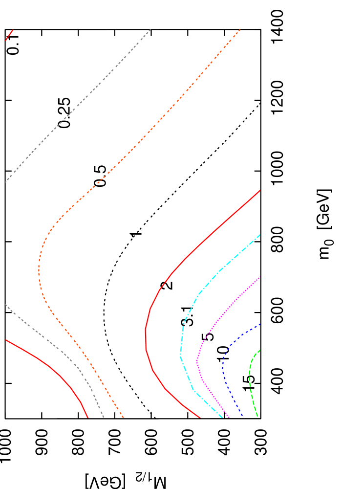
Figure 7: Contour plot of BR$(\tau\to\mu\gamma)$ in the $m_{0}-M_{1/2}$ plane with $\mu=120$ GeV and $A_{0}=0$. Contours are in units of $10^{-7}$, the present experimental bound marked as ”3.1”.

An experimental lower bound on each sparticle mass was imposed. In particular, the most constraining are: the LEP limits on the charged SUSY masses ($m_{\tilde{\chi}^{\pm}},m_{\tilde{\tau}}>105$ GeV), the CDF limit on the mass of the $CP$ odd Higgs state ($m_{A^{0}}>105$-$110\,$ GeV, valid for $\tan\beta\approx 50$)[38], and the requirement that the lightest SUSY particle should be neutral. Finally, a $\chi^{2}$ function, $\;\sum_{i}\;(X_{i}^{th}-X_{i}^{exp})^{2}/\sigma_{i}^{2}\;$, is evaluated based on the agreement between the theoretical predictions and 24 experimental observables collected in table 1. The numerical procedure described above was previously exploited to study lepton flavour violation, the muon anomalous magnetic moment, neutrino oscillations and $b\to s\gamma$ within supersymmetric Pati-Salam[21, 39] and $SO(10)$[35, 40] models.

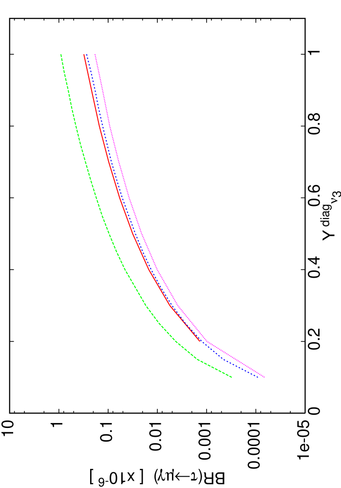
Figure 8: Variation of the BR$(\tau\to\mu\gamma)$ as the third generation Neutrino Yukawa coupling ranges from 0.1 to 1.0.

For our analysis we selected 100 evenly spaced points in the SUSY parameter space each with values of $m_{0}$ and $M_{1/2}$ in the plane, $m_{0}=300-1400$ GeV and $M_{1/2}=300-1000$ GeV. For each of the 100 points we also held fixed $\mu=120$ GeV, $\tan\beta=50$ and $A_{0}=0$. The remaining input parameters of eq. (75) are allowed to vary in order to find the minimum of our electroweak $\chi^{2}$ function. The results of our analysis are discussed in the following section.

5 Discussion

In the previous section we outlined the numerical procedure used to analyse 100 points in the SUSY $m_{0}-M_{1/2}$ plane. In our analysis of these points we have kept fixed $\mu=120$ GeV, $\tan\beta=50$ and $A_{0}=0$. In this section we shall present in detail the results of our analysis.

5.1 Lepton flavour violating $\mu\to e\gamma$ and $\tau\to\mu\gamma$

Let us firstly look at the important lepton flavour violating decay $\tau\to\mu\gamma$. A contour plot showing the variation of the branching ratio for $\tau\to\mu\gamma$ in the $m_{0}-M_{1/2}$ plane is given in fig. 7. This plot shows that the rate for this process is very high over most of the plane and even in the low $m_{0}-M_{1/2}$ region the rate can exceed the present experimental upper bound. These large rates are a direct consequence of our choice of $Y_{\nu_{3}}=0.6$. It is interesting therefore to notice the variation of the rate for $\tau\to\mu\gamma$ with the size of $Y_{\nu_{3}}$ as shown in fig. 8. In this plot we have allowed $Y_{\nu_{3}}$ to vary from 0.1 to 1.0 whilst observing the resulting change in the rate for $\tau\to\mu\gamma$. We observed this variation for a small number of fixed points in the $m_{0}-M_{1/2}$ plane, as noted in the figure. It is interesting to notice that the decay rate changes by about three orders of magnitude whilst the Yukawa coupling varies by just a single order of magnitude. This type of $Y_{\nu}$ dependence clearly comes from the dependence of $\Delta m_{\tilde{L}}^{2}$ shown eq. 24, which shows that $(\Delta m_{\tilde{L}}^{2})_{23}$ has a roughly $(Y_{\nu_{3}}^{\rm diag})^{2}$ dependence.

Figure 9: BR$(\mu\to e\gamma)$ plotted against the Pseudoscalar Higgs mass, $m_{A^{0}}$.

On the other hand, the rate for the decay $\mu\to e\gamma$ appears to be much more suppressed. Our results, plotted in fig. 9 against the Pseudoscalar Higgs mass, show that for small values of $m_{A^{0}}$ the rate is highly variable over the range $10^{-18}-10^{-11}$. At larger values of $m_{A^{0}}$ a slight bunching of points appears to occur in a narrow horizontal band. It seems that our model prefers a $\mu\to e\gamma$ rate in the region $10^{-15}-10^{-14}$, which is close to the search limitations of the present MEG experiment[8].

5.2 Higgs mediated $B_{s}\to\mu\mu$, $B_{s}\to\tau\mu$, $\tau\to 3\mu$ and $\Delta M_{s}$

The plots for the Higgs mediated contribution to the flavour changing neutral current decay, $B_{s}\to\mu\mu$, are presented in fig. 10b. As previously reported by a number of authors[13, 26] the branching ratio for $B_{s}\to\mu\mu$ is particularly interesting with rates ranging from $10^{-10}$ for heavy $m_{A^{0}}$ up to almost $10^{-5}$ for a particularly light $m_{A^{0}}$. The present $90\%$ C.L. experimental upper bound of $0.8\times 10^{-7}$[14] excludes the highest predicted rates and hence is beginning to probe the Higgs sector into the region $m_{A^{0}}\sim 150$ GeV. This rare decay is certainly of particular interest and future studies will continue to probe the Higgs sector to an even greater extent. Within the standard model the expectation is that Br$(B_{s}\to\mu\mu)_{SM}\sim 10^{-9}$. Therefore we can see from fig. 10b that the Higgs mediated contribution to this process would dominate as long as $m_{A^{0}}<500$ GeV and this decay has the possibility of being the first indirect signal of supersymmetry.

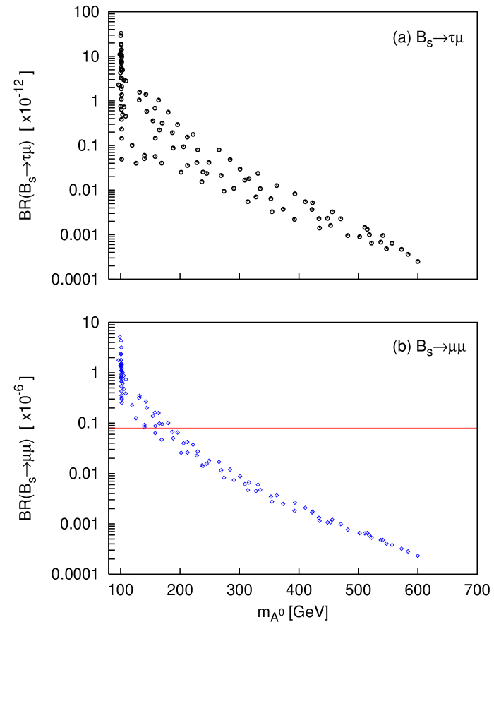
Figure 10: The Higgs mediated contribution to Br$(B_{s}\to\mu\mu,\tau\mu)$ plotted against the Pseudoscalar Higgs mass. In figure (b) the horizontal line at $0.8\times 10^{-7}$ shows the present $90\%$ C.L. experimental upper bound [14].

The lepton flavour violating decay $B_{s}\to\tau\mu$ is plotted in fig. 10a against the Pseudoscalar Higgs mass. This plot shows that the branching ratio for this decay could be as large as $\sim 10^{-10}$, but is certainly not as interesting as the flavour conserving decay just discussed. The branching ratio for the decay $\tau\to\mu\mu\mu$ is of a similar order of magnitude to that in fig. 10a. These rates are not quite as high as those reported in eq. (12) and (13).

In the limit of large $\tan\beta$, $B_{s}\to\mu^{+}\mu^{-}$ and $\Delta M_{s}$ are correlated. This correlation is shown in the two panels of fig. 11. For these two panels the two different values of $f_{B_{s}}$ listed in eq. (45) and (46) are used. The upper panel ($f_{B_{s}}=230$ MeV) shows that the central value of $(\Delta M_{s}^{\rm CDF}-\Delta M_{s}^{\rm SM})$ coincides with the bound from Br$(B_{s}\to\mu^{+}\mu^{-})$. The lower panel ($f_{B_{s}}=259$ MeV) shows that the data points with $\Delta M_{s}^{\rm DP}$ at the central value, are in fact ruled out by the bound on Br$(B_{s}\to\mu^{+}\mu^{-})$. The uncertainty in the SM prediction for $\Delta M_{s}$ is rather large and in fact all of the data points of fig. 11 agree with the recent Tevatron measurement to within $1\sigma$. These two panels clearly show that the interpretation of the recent measurement depends crucially on the uncertainty in the determination of $f_{B_{s}}$.

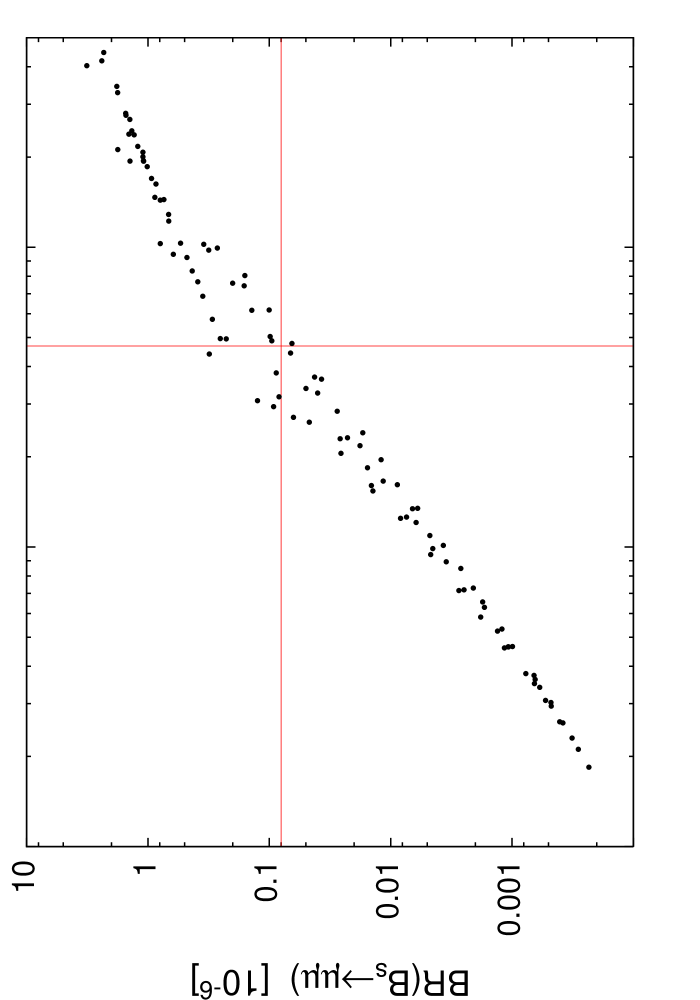
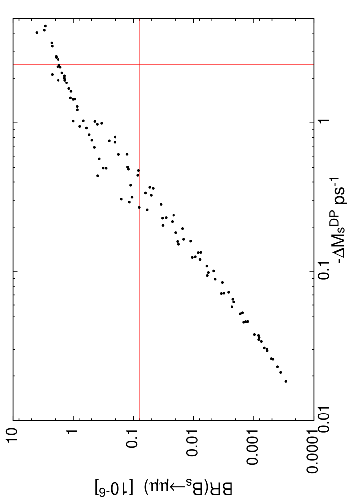
Figure 11: The correlation of Br$(B_{s}\to\mu^{+}\mu^{-})$ and $\Delta M_{s}^{\rm DP}$ are given for $f_{B_{s}}=230$ MeV (upper panel) and $f_{B_{s}}=259$ MeV(lower panel). The horizontal line in both panels shows the present experimental bound on Br$(B_{s}\to\mu^{+}\mu^{-})$. The vertical lines mark the central value of $(\Delta M_{s}^{\rm CDF}-\Delta M_{s}^{SM})$.

Figure 12: Plot for the ratio, $\Delta M_{s}^{LL}/\Delta M_{s}^{LR}$, of the Higgs contribution to the operators $Q_{1}^{SLL}$ and $Q_{2}^{LR}$.

The plot in fig. 12 shows the ratio, $\Delta M_{s}^{LL}/\Delta M_{s}^{LR}$, of the contributions to the operators $Q_{1}^{\rm SLL}$ and $Q_{2}^{\rm LR}$ as defined in eq. (3.1). It is commonly assumed that the contribution to the $Q_{1}^{\rm SLL}$ operator, $\Delta M_{s}^{LL}$, is negligible. From fig. 12 we can see that the contribution of the $Q_{1}^{\rm SLL}$ operator, $\Delta M_{s}^{LL}$, is between 40% and 90% of $\Delta M_{s}^{LR}$ and hence is significant.

5.3 Lepton flavour violating decays of MSSM Higgs bosons

Our numerical results for the branching ratio of $H^{0}\to\tau\mu$ are presented in fig. 13c. The rates for this process are plotted against the Pseudoscalar Higgs mass, $m_{A^{0}}$. The predicted rates range from $10^{-9}$ up to a few times $10^{-7}$. In fig. 13c we can see a broad band of points stretching from $m_{A^{0}}=100$ GeV up to $m_{A^{0}}=600$ GeV showing that most points are predicting a rate of around $10^{-8}$. The decay rate appears to be almost independent of the Pseudoscalar Higgs mass, although there is a slight peak at the lower range of the Higgs mass, which is where the highest rates are achieved. Notice that the data points shown in fig. 13 are divided into two groups. The grouping is determined by whether the $B_{s}\to\mu\mu$ bound is in excess or not, as indicated in the figure caption. From this grouping we can see that the points with the highest predicted $H^{0}\to\tau\mu$ rates appear to be excluded by the $B_{s}\to\mu\mu$ bound. In this way the Higgs mediated contribution to the $B_{s}$ decay can provide additional information on the allowed Higgs decay rate.

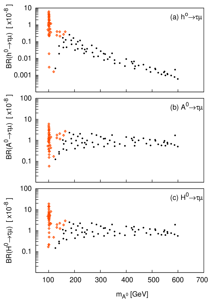
Figure 13: BR($h^{0},A^{0},H^{0}\to\tau\mu$) plotted against $m_{A^{0}}$. Each of the scatter points represent the output result from an fixed value in $M_{1/2}$ and $m_{0}$. For each of these fitted points we have assumed, $\mu=120$ GeV and $A_{0}=0$. Here the dots(diamonds) mark points for which $Br(B_{s}\to\mu\mu)$ is below(above) the present experimental limit.

Fig. 13b shows our predictions for the lepton flavour violating Pseudoscalar Higgs decay, $A^{0}\to\tau\mu$. The rates for the decay of the Pseudoscalar are almost identical to those of the heavy CP-even Higgs shown in fig. 13.

The rate for the decay of the lightest Higgs boson is shown in fig. 13a where it is again plotted against the Pseudoscalar Higgs mass. The predicted rates for this decay show a very different dependence upon $m_{A^{0}}$, as they are spread over a large range from $10^{-11}$ to $10^{-7}$. The branching ratio for the lightest Higgs appears to be inversely proportional to the Pseudoscalar Higgs mass. Hence this LFV decay will only be interesting if $m_{A^{0}}<300$ GeV where its rate can be comparable to those for the other neutral Higgs states. The data points for the lightest Higgs boson decay of fig. 13a have again been divided into two groups. As before, the two groupings depend upon whether the $B_{s}\to\mu\mu$ bound is being exceeded or not. The plot shows that the data points for particularly light Pseudoscalar Higgs mass are excluded by the $B_{s}\to\mu\mu$ bound. These excluded points correspond to the largest predictions for the decay $h^{0}\to\tau\mu$ and leaves, $3\times 10^{-9}$, the highest allow decay rate.

Figure 14: Br$(H^{0}\to\tau\mu)$ plotted against Br$(\tau\to\mu\gamma)$.

Fig. 14 shows the correlation between the two LFV decays $H^{0}\to\tau\mu$ and $\tau\to\mu\gamma$. The plot shows a very nice linear relation between the two branching ratios. The rate for $\tau\to\mu\gamma$ is generally a factor of $\sim 10$ larger than that for $H^{0}\to\tau\mu$, although there is a region towards the bottom left of the plot where the two rates become comparable.

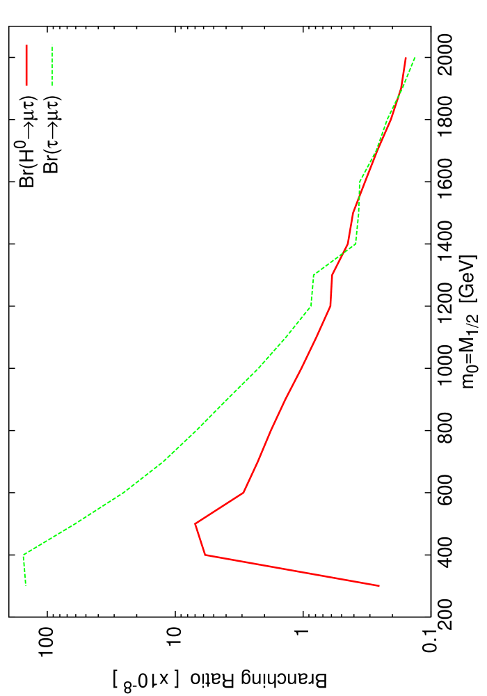
Figure 15: Br$(H\to\tau\mu)$ and Br$(\tau\to\mu\gamma)$ plotted along the line $m_{0}=M_{1/2}$.

In some other works[12] a non-decoupling effect in the Higgs decay $H^{0}\to\tau\mu$ was observed. It was found that the decay $\tau\to\mu\gamma$ experiences a decoupling suppression for large values of $m_{0}$ and $M_{1/2}$. This decoupling is experienced as a result of heavy SUSY particles in the loops of lepton flavour violating diagrams. On the other hand the Higgs LFV coupling do not experience such a large suppression. It was noted that, in this decoupling region, the LFV Higgs decay rate can be larger than the tau decay rate.

In order to examine such an effect we present a plot of the two decay rates against $m_{0}=M_{1/2}$, see fig. 14. We see that the rate for the tau decay is initially an order of magnitude greater than that for the Higgs decay. As we move from small to large values of $m_{0}=M_{1/2}$ the rate for the tau decay falls sharply where as the rate for the Higgs decay falls less sharply. By the time we reach $m_{0}=M_{1/2}=2000$ GeV we find that the two rates have become comparable and the Higgs decay rate may even become marginally larger than that for the tau decay. Other authors noted a greater shift than we have found, with the Higgs decay rate becoming $\sim 6$ times greater than the tau decay rate. Here we did not see such an large effect at large values of $m_{0}=M_{1/2}$.

6 Conclusions

We have analysed a supersymmetric model constrained by $SU(5)$ unification with right-handed neutrinos providing light neutrino masses via the seesaw mechanism. We have been concerned with making predictions for lepton flavour violating decay processes such as $\tau\to\mu\gamma$, $\mu\to e\gamma$ and $\phi^{0}\to\tau\mu$. With lepton flavour violation in mind, we chose to study the large $\tan\beta$ region of parameter space where such effects are enhanced. In addition we chose $Y_{\nu_{3}}\sim 1$ under the influence of $SO(10)$ unification in which $\tan\beta$ is naturally large.

Our numerical procedure utilises a complete top-down global $\chi^{2}$ fit to 24 low-energy observables. Through this electroweak fit we were able to analyse lepton flavour violating decay rates for rare charged lepton decays. The choice of a large third family neutrino Yukawa coupling naturally leads to large 23 lepton flavour violation. Within this scenario we have also used our numerical fits to analyse the branching ratios for the FCNC processes $B_{s}\to\mu\mu$, $B_{s}\to\tau\mu$ and the lepton flavour violating decays of MSSM Higgs bosons. As a result, we have been able to make realistic predictions for these decays while ensuring the maximum $\tau-\mu$ violation allowed by the present $\tau\to\mu\gamma$ constraint.

Our model predicts a $\tau\to\mu\gamma$ rate in the region $(10^{-8}-10^{-6})$ and a $\mu\to e\gamma$ rate in the region $(10^{-15}-10^{-14})$. We have seen that the branching ratio for $H^{0}\to\tau\mu$ could be particularly interesting with a rate as high as few $10^{-7}$. We also saw that in the large $m_{0}-M_{1/2}$ region of parameter space this branching ratio could become comparable to that for $\tau\to\mu\gamma$. The Higgs mediated contribution to the branching ratio for $B_{s}\to\mu\mu$ was found to be particularly large and could even exceed the current experimental bound. In addition to the constraint of $\tau\to\mu\gamma$, we also saw that the $B_{s}\to\mu\mu$ bound may also act as a stringent restriction on the allowed rates for $\phi^{0}\to\tau\mu$. We found the rates for the LFV decays $B_{s}\to\tau\mu$ and $\tau\to\mu\mu\mu$ are rather small $<10^{-10}$.

The correlation of $B_{s}\to\mu^{+}\mu^{-}$ and $\Delta M_{s}$ in the large $\tan\beta$ limit was also studied. The constraint from the recent Tevatron measurement is highly dependent upon the determination of $f_{B_{s}}$. It was found that the Higgs contribution to the often neglected operator $Q_{1}^{\rm SLL}$ may be as large as $90\%$ of the contribution from the operator $Q_{2}^{\rm LR}$. Therefore the operator $Q_{1}^{\rm SLL}$ is certainly non-negligible.

References

- [1] Y. Fukuda et al. [Super-Kamiokande Collaboration], Phys. Rev. Lett. 81 (1998) 1562 [arXiv:hep-ex/9807003]. Y. Fukuda et al. [Super-Kamiokande Collaboration], Phys. Lett. B 436 (1998) 33 [arXiv:hep-ex/9805006].
- [2] Q. R. Ahmad et al. [SNO Collaboration], Phys. Rev. Lett. 89 (2002) 011301 [arXiv:nucl-ex/0204008]; Q. R. Ahmad et al. [SNO Collaboration], Phys. Rev. Lett. 89 (2002) 011302 [arXiv:nucl-ex/0204009].
- [3] M. H. Ahn et al. [K2K Collaboration], Phys. Rev. Lett. 90 (2003) 041801 [arXiv:hep-ex/0212007].
- [4] K. Eguchi et al. [KamLAND Collaboration], Phys. Rev. Lett. 90 (2003) 021802 [arXiv:hep-ex/0212021].
- [5] G. L. Fogli, E. Lisi, A. Marrone, A. Palazzo and A. M. Rotunno, arXiv:hep-ph/0506307. G. L. Fogli, E. Lisi, A. Marrone and A. Palazzo, arXiv:hep-ph/0506083.
- [6] M. L. Brooks et al. [MEGA Collaboration], Phys. Rev. Lett. 83 (1999) 1521 [arXiv:hep-ex/9905013].
- [7] K. Hayasaka [Belle Collaboration], Nucl. Phys. Proc. Suppl. 144 (2005) 149.
- [8] M. Grassi [MEG Collaboration], Nucl. Phys. Proc. Suppl. 149 (2005) 369. S. Yamada, Nucl. Phys. Proc. Suppl. 144 (2005) 185. A. Baldini, AIP Conf. Proc. 721 (2004) 289.
- [9] A. Dedes, J. R. Ellis and M. Raidal, Phys. Lett. B 549 (2002) 159 [arXiv:hep-ph/0209207]. D. Guetta, J. M. Mira and E. Nardi, Phys. Rev. D 59 (1999) 034019 [arXiv:hep-ph/9806359].
- [10] K. S. Babu and C. Kolda, Phys. Rev. Lett. 89 (2002) 241802 [arXiv:hep-ph/0206310].
- [11] M. Sher, Phys. Rev. D 66 (2002) 057301 [arXiv:hep-ph/0207136].
- [12] J. L. Diaz-Cruz and J. J. Toscano, Phys. Rev. D 62 (2000) 116005 [arXiv:hep-ph/9910233]. J. L. Diaz-Cruz, JHEP 0305 (2003) 036 [arXiv:hep-ph/0207030]. U. Cotti, M. Pineda and G. Tavares-Velasco, arXiv:hep-ph/0501162. A. Brignole and A. Rossi, Phys. Lett. B 566 (2003) 217 [arXiv:hep-ph/0304081]. A. Brignole and A. Rossi, Nucl. Phys. B 701 (2004) 3 [arXiv:hep-ph/0404211]. E. Arganda, A. M. Curiel, M. J. Herrero and D. Temes, Phys. Rev. D 71 (2005) 035011 [arXiv:hep-ph/0407302]. S. Kanemura, K. Matsuda, T. Ota, T. Shindou, E. Takasugi and K. Tsumura, Phys. Lett. B 599 (2004) 83 [arXiv:hep-ph/0406316]. S. Kanemura, T. Ota and K. Tsumura, arXiv:hep-ph/0505191.
- [13] C. S. Huang, W. Liao and Q. S. Yan, Phys. Rev. D 59, 011701 (1999) [arXiv:hep-ph/9803460]. S. R. Choudhury and N. Gaur, Phys. Lett. B 451 (1999) 86 [arXiv:hep-ph/9810307]. K. S. Babu and C. F. Kolda, Phys. Rev. Lett. 84, 228 (2000) [arXiv:hep-ph/9909476]. C. S. Huang, W. Liao, Q. S. Yan and S. H. Zhu, Phys. Rev. D 63, 114021 (2001) [Erratum-ibid. D 64, 059902 (2001)] [arXiv:hep-ph/0006250]. P. H. Chankowski and L. Slawianowska, Phys. Rev. D 63, 054012 (2001) [arXiv:hep-ph/0008046]. C. Bobeth, T. Ewerth, F. Kruger and J. Urban, Phys. Rev. D 64, 074014 (2001) [arXiv:hep-ph/0104284]. A. Dedes, H. K. Dreiner and U. Nierste, Phys. Rev. Lett. 87, 251804 (2001) [arXiv:hep-ph/0108037]. G. Isidori and A. Retico, JHEP 0111, 001 (2001) [arXiv:hep-ph/0110121]. R. Arnowitt, B. Dutta, T. Kamon and M. Tanaka, Phys. Lett. B 538, 121 (2002) [arXiv:hep-ph/0203069]. C. Bobeth, T. Ewerth, F. Kruger and J. Urban, Phys. Rev. D 66, 074021 (2002) [arXiv:hep-ph/0204225]. A. Dedes, H. K. Dreiner, U. Nierste and P. Richardson, arXiv:hep-ph/0207026. A. J. Buras, P. H. Chankowski, J. Rosiek and L. Slawianowska, Phys. Lett. B 546, 96 (2002) [arXiv:hep-ph/0207241]. J. K. Mizukoshi, X. Tata and Y. Wang, Phys. Rev. D 66, 115003 (2002) [arXiv:hep-ph/0208078]. S. Baek, P. Ko and W. Y. Song, JHEP 0303, 054 (2003) [arXiv:hep-ph/0208112]. G. Isidori and A. Retico, JHEP 0209, 063 (2002) [arXiv:hep-ph/0208159]. A. Dedes and A. Pilaftsis, Phys. Rev. D 67 (2003) 015012 [arXiv:hep-ph/0209306]. C. S. Huang and X. H. Wu, Nucl. Phys. B 657, 304 (2003) [arXiv:hep-ph/0212220]. T. Hurth, arXiv:hep-ph/0212304. T. Kamon [CDF Collaboration], arXiv:hep-ex/0301019. D. A. Demir, arXiv:hep-ph/0303249. R. Dermisek, S. Raby, L. Roszkowski and R. Ruiz De Austri, JHEP 0304, 037 (2003) [arXiv:hep-ph/0304101]. T. Blazek, S. F. King and J. K. Parry, Phys. Lett. B 589 (2004) 39 [arXiv:hep-ph/0308068]. G. L. Kane, C. Kolda and J. E. Lennon, arXiv:hep-ph/0310042. S. Baek, Phys. Lett. B 595 (2004) 461 [arXiv:hep-ph/0406007]. S. Baek, Y. G. Kim and P. Ko, 0502 (2005) 067 [arXiv:hep-ph/0406033]. A. Dedes and B. T. Huffman, Phys. Lett. B 600 (2004) 261 [arXiv:hep-ph/0407285]. J. R. Ellis, K. A. Olive and V. C. Spanos, arXiv:hep-ph/0504196. S. Baek, Y. G. Kim and P. Ko, arXiv:hep-ph/0506115. R. Dermisek, S. Raby, L. Roszkowski and R. Ruiz de Austri, arXiv:hep-ph/0507233.
- [14] CDF Collaboration, CDF Public Note 8176, www-cdf.fnal.gov
- [15] H. Georgi and C. Jarlskog, Phys. Lett. B 86, 297 (1979).
- [16] J. Hisano and Y. Shimizu, Phys. Lett. B 565 (2003) 183 [arXiv:hep-ph/0303071]. N. Akama, Y. Kiyo, S. Komine and T. Moroi, Phys. Rev. D 64 (2001) 095012 [arXiv:hep-ph/0104263]. J. Hisano, M. Kakizaki, M. Nagai and Y. Shimizu, Phys. Lett. B 604, 216 (2004) [arXiv:hep-ph/0407169]. D. Chang, A. Masiero and H. Murayama, Phys. Rev. D 67 (2003) 075013 [arXiv:hep-ph/0205111].
- [17] J. Hisano, T. Moroi, K. Tobe, M. Yamaguchi and T. Yanagida, B 357 (1995) 579 [arXiv:hep-ph/9501407]. J. Hisano, T. Moroi, K. Tobe and M. Yamaguchi, Phys. Rev. D 53 (1996) 2442 [arXiv:hep-ph/9510309].
- [18] A. Masiero, S. K. Vempati and O. Vives, Nucl. Phys. B 649 (2003) 189 [arXiv:hep-ph/0209303].
- [19] S. F. King and M. Oliveira, Phys. Rev. D 60 (1999) 035003 [arXiv:hep-ph/9804283].
- [20] T. Blažek and S. F. King, Phys. Lett. B 518 (2001) 109 [arXiv:hep-ph/0105005].
- [21] T. Blažek and S. F. King, arXiv:hep-ph/0211368.
- [22] F. Borzumati and A. Masiero, Phys. Rev. Lett. 57 (1986) 961. J. Hisano and D. Nomura, Phys. Rev. D 59 (1999) 116005 [arXiv:hep-ph/9810479]. J. R. Ellis, M. E. Gomez, G. K. Leontaris, S. Lola and D. V. Nanopoulos, Eur. Phys. J. C 14 (2000) 319 [arXiv:hep-ph/9911459]. S. Lavignac, I. Masina and C. A. Savoy, Phys. Lett. B 520 (2001) 269 [arXiv:hep-ph/0106245]. J. A. Casas and A. Ibarra, Nucl. Phys. B 618 (2001) 171 [arXiv:hep-ph/0103065]. T. Fukuyama, T. Kikuchi and N. Okada, Phys. Rev. D 68, 033012 (2003) [arXiv:hep-ph/0304190]. T. Fukuyama, A. Ilakovac and T. Kikuchi, arXiv:hep-ph/0506295.
- [23] R. Hempfling, Phys. Rev. D49, 6168 (1994). L. Hall, R. Rattazzi and U. Sarid, Phys. Rev. D50, 7048 (1994). M. Carena, M. Olechowski, S. Pokorski and C. Wagner, Nucl. Phys. B426, 269 (1994).
- [24] T. Blazek, S. Raby and S. Pokorski, Phys. Rev. D 52, 4151 (1995) [arXiv:hep-ph/9504364].
- [25] C. Hamzaoui, M. Pospelov and M. Toharia, Phys. Rev. D 59, 095005 (1999) [arXiv:hep-ph/9807350].
- [26] A. J. Buras, P. H. Chankowski, J. Rosiek and L. Slawianowska, Nucl. Phys. B 659 (2003) 3 [arXiv:hep-ph/0210145]. A. J. Buras, P. H. Chankowski, J. Rosiek and L. Slawianowska, Phys. Lett. B 546 (2002) 96 [arXiv:hep-ph/0207241].
- [27] S. Hashimoto, Int. J. Mod. Phys. A 20 (2005) 5133 [arXiv:hep-ph/0411126].
- [28] A. Gray et al. [HPQCD Collaboration], Phys. Rev. Lett. 95 (2005) 212001 [arXiv:hep-lat/0507015].
- [29] A. Abulencia [CDF - Run II Collaboration], arXiv:hep-ex/0606027. V. M. Abazov et al. [D0 Collaboration], arXiv:hep-ex/0603029.
- [30] A. Djouadi, J. Kalinowski and M. Spira, Comput. Phys. Commun. 108 (1998) 56 [arXiv:hep-ph/9704448].
- [31] B. Aubert et al. [BABAR Collaboration], Phys. Rev. Lett. 92 (2004) 121801 [arXiv:hep-ex/0312027].
- [32] Y. Enari et al. [Belle Collaboration], Phys. Rev. Lett. 93 (2004) 081803 [arXiv:hep-ex/0404018].
- [33] B. Aubert et al. [BABAR Collaboration], Phys. Rev. Lett. 94 (2005) 221803.
- [34] J. E. Duboscq, Nucl. Phys. Proc. Suppl. 144 (2005) 265 [arXiv:hep-ex/0412022].
- [35] T. Blažek, M. Carena, S. Raby and C.E.M. Wagner, Phys. Rev. D 56 (1997) 6919 [arXiv:hep-ph/9611217].
- [36] P. Shagin et al. [E821 Collaboration], eConf C040802 (2004) TUT007. T. Teubner, Prepared for 12th International Workshop on Deep Inelastic Scattering (DIS 2004), Strbske Pleso, Slovakia, 14-18 Apr 2004
- [37] M.Carena, J.R. Espinosa, M.Quiros and C. Wagner, Phys. Lett. B355, 209 (1995); M.Carena, M.Quiros and C. Wagner, Nucl. Phys. B461, 407 (1996); J.A. Casas, J.R. Espinosa, M. Quiros and A. Riotto, Nucl. Phys. B436, 3 (1995).
- [38] T. Affolder et al. [CDF Collaboration], Phys. Rev. Lett. 86 (2001) 4472 [arXiv:hep-ex/0010052].
- [39] T. Blazek, S. F. King and J. K. Parry, JHEP 0305 (2003) 016 [arXiv:hep-ph/0303192].
- [40] T. Blazek, R. Dermisek and S. Raby, Phys. Rev. D 65 (2002) 115004 [arXiv:hep-ph/0201081]. T. Blazek, R. Dermisek and S. Raby, Phys. Rev. Lett. 88 (2002) 111804 [arXiv:hep-ph/0107097]. T. Blazek, S. Raby and K. Tobe, Phys. Rev. D 62 (2000) 055001 [arXiv:hep-ph/9912482]. T. Blazek, arXiv:hep-ph/9912460. T. Blazek, M. Carena, S. Raby and C. E. M. Wagner, Phys. Rev. D 56 (1997) 6919 [arXiv:hep-ph/9611217].