Abstract

We examine the possibility of detecting signals of split supersymmetry in the loop-induced decay $h\longrightarrow\gamma\gamma$ of the Higgs boson at the Large Hadron Collider, where charginos, as surviving light fermions of the supersymmetric spectrum, can contribute in the loop. We perform a detailed study of uncertainties in various parameters involved in the analysis, and thus the net uncertainty in the standard model prediction of the rate. After a thorough scan of the parameter space, taking all constraints into account, we conclude that it will be very difficult to infer about split supersymmetry from Higgs signals alone.

1 Introduction

The idea of a supersymmetric nature, with supersymmetry (SUSY) broken in a phenomenologically consistent manner, is several decades old now. It is expected that the Large Hadron Collider (LHC) will reveal its trace if the scale of SUSY breaking is within a TeV or so. In addition, signals for the Higgs boson(s) at the LHC are also likely to yield useful information about SUSY. For example, in the minimal SUSY standard model (MSSM) and most of its extensions, the lightest neutral Higgs has a mass within about 135 GeV. Furthermore, its couplings with the standard model particles differ from the standard model values, and such departure can be tested at the LHC and more precisely at a linear collider, giving us an indication about a supersymmetric world from the Higgs signals themselves.

The situation is somewhat different in split SUSY, a recently proposed scenario where all supersymmetric scalars are very heavy while the gauginos and Higgsinos can be within the TeV scale [1, 2]. Such a scenario is motivated by the fact that an inadmissibly large cosmological constant is difficult to avoid in a broken SUSY model, unless one fine-tunes parameters to a high degree. Therefore, it has been argued, it may not be out of place to stabilize the electroweak (EW) scale, too, via fine tuning. Nonetheless, SUSY as an artifact of theories such as superstring may still be around, albeit with a large breaking scale.

Since it does not claim to solve the hierarchy problem, split SUSY can have the scalar masses (and the SUSY breaking scale) as high as $10^{13}$ GeV or so. It avoids the problems with flavor changing neutral current plaguing the usual SUSY models, still provides a dark matter candidate, and even offers to retain gauge coupling through TeV-scale thresholds consisting of incomplete representations of the Grand Unification group [2]. Thus, although the very philosophy underlying split SUSY may be questioned, it is important to explore its observable consequences. In particular, one would always like to see if the Higgs sector still contains information on new physics. The problem is that in the split SUSY scenario, the low-energy spectrum contains only one neutral Higgs, its interaction strength with all standard model particles being exactly as in the standard model itself. This makes it difficult to distinguish split SUSY from signals of the Higgs boson, at least in tree-level processes, since such processes are unlikely to produce SUSY particles from decays of the Higgs.

It has been suggested earlier [3] that it may be possible to recognize a Higgs in such a case through its loop-induced decays. In particular, the decay channel $h\longrightarrow\gamma\gamma$ gets additional contributions from chargino loops. If these contributions are substantial, then it may be possible, it has been argued, to seek the signature of split SUSY in the two-photon decay channel of the Higgs boson, even before the accessible part of the SUSY spectrum reveals itself.

However, the difference made by charginos in the loop-induced effects needs to be analyzed with the full process of Higgs production and its subsequent decay in mind. The authors themselves noted in passing in reference [3], that the error in measurements might be substantial at the LHC. Nonetheless, it requires a thorough analysis of the various parameters involved, in order to ascertain whether split SUSY could leave its mark on Higgs decay in the most energetic high energy collider approved till now. In this paper we carry out such an analysis, taking into account all uncertainties in experimental measurements as well as theoretical predictions. Thereafter we make a thorough scan of the split SUSY parameter space, looking for regions where the chargino contributions in the loop could stand out against other uncertainties in the observed event rates. Our conclusion is that it may be difficult to be sure of any split SUSY contributions over most of the parameter space of one’s interest.

In section 2 we outline the relevant features of split SUSY. In section 3 we take up signals for the Higgs boson, where the diphoton decay mode and the relevant procedure for predicting it are discussed. The various uncertainties in the standard model prediction, relevant for our study, are listed in section 4, while section 5 contains the results of a numerical scan of the parameter space. We summarise and conclude in section 6.

2 The split SUSY spectrum

As has been mentioned in the previous section, this scenario introduces a splitting between scalars and the fermions. This means, all the squarks and sleptons as well as all physical states in the electroweak symmetry breaking sector excepting one are ultra-heavy, while gauginos, Higgsinos and one (finely-tuned) neutral Higgs boson remain light.

The low-energy spectrum of split SUSY can be obtained by writing the most general renormalizable Lagrangian [2] where the heavy scalars have been integrated out and only one Higgs doublet $(H)$ is retained:

$${\cal L} = m^{2}H^{\dagger}H-\frac{\lambda}{2}\left(H^{\dagger}H\right)^{2}-\left[h^{u}_{ij}{\bar{q}}_{j}u_{i}\epsilon H^{*}+h^{d}_{ij}{\bar{q}}_{j}d_{i}H+h^{e}_{ij}{\bar{\ell}}_{j}e_{i}H\right.$$ (1)

$$+\frac{M_{3}}{2}{\tilde{g}}^{A}{\tilde{g}}^{A}+\frac{M_{2}}{2}{\tilde{W}}^{a}{\tilde{W}}^{a}+\frac{M_{1}}{2}{\tilde{B}}{\tilde{B}}+\mu{\tilde{H}}_{u}^{T}\epsilon{\tilde{H}}_{d}$$

$$\left.+\frac{H^{\dagger}}{\sqrt{2}}\left({\tilde{g}}_{u}\sigma^{a}{\tilde{W}}^{a}+{\tilde{g}}_{u}^{\prime}{\tilde{B}}\right){\tilde{H}}_{u}+\frac{H^{T}\epsilon}{\sqrt{2}}\left(-{\tilde{g}}_{d}\sigma^{a}{\tilde{W}}^{a}+{\tilde{g}}_{d}^{\prime}{\tilde{B}}\right){\tilde{H}}_{d}+{\rm h.c.}\right],$$

where $\epsilon=i\sigma_{2}$ and ${\tilde{H}}_{u,d}$ (Higgsinos), $\tilde{g}$ (gluino), $\tilde{W}$ (W-ino), $\tilde{B}$ (B-ino) are the gauginos.

The coupling strengths of the effective theory at the scale ${m_{S}}$, where ${m_{S}}$ is the scale of SUSY breaking, are obtained by matching the Lagrangian in equation 1. with the interaction terms of the supersymmetric Higgs doublets $H_{u}$ and $H_{d}$:

$${\cal L}_{\rm susy} = -\frac{g^{2}}{8}\left(H_{u}^{\dagger}\sigma^{a}H_{u}+H_{d}^{\dagger}\sigma^{a}H_{d}\right)^{2}-\frac{g^{\prime 2}}{8}\left(H_{u}^{\dagger}H_{u}-H_{d}^{\dagger}H_{d}\right)^{2}$$ (2)

$$+Y^{u}_{ij}H_{u}^{T}\epsilon{\bar{u}}_{i}q_{j}-Y^{d}_{ij}H_{d}^{T}\epsilon{\bar{d}}_{i}q_{j}-Y^{e}_{ij}H_{e}^{T}\epsilon{\bar{e}}_{i}\ell_{j}$$

$$-\frac{H_{u}^{\dagger}}{\sqrt{2}}\left(g\sigma^{a}{\tilde{W}}^{a}+g^{\prime}{\tilde{B}}\right){\tilde{H}}_{u}-\frac{H_{d}^{\dagger}}{\sqrt{2}}\left(g\sigma^{a}{\tilde{W}}^{a}-g^{\prime}{\tilde{B}}\right){\tilde{H}}_{d}+{\rm h.c.}$$

The combination $H=-\cos\beta\epsilon H_{d}^{*}+\sin\beta H_{u}$ is then fine-tuned to have a small mass term. The matching conditions for the coupling constants in equation 1. at the scale ${m_{S}}$ are obtained by replacing $H_{u}\to\sin\beta H$, $H_{d}\to\cos\beta\epsilon H^{*}$ in equation 2.:

$$\lambda(m_{S}) = \frac{\left[g^{2}(m_{S})+g^{\prime 2}(m_{S})\right]}{4}\cos^{2}2\beta,$$ (3)

$$h^{u}_{ij}(m_{S})=Y^{u*}_{ij}(m_{S})\sin\beta, h^{d,e}_{ij}(m_{S})=Y^{d,e*}_{ij}(m_{S})\cos\beta,$$ (4)

$${\tilde{g}}_{u}(m_{S})=g(m_{S})\sin\beta, {\tilde{g}}_{d}(m_{S})=g(m_{S})\cos\beta,$$ (5)

$${\tilde{g}}_{u}^{\prime}(m_{S})=g^{\prime}(m_{S})\sin\beta, {\tilde{g}}_{d}^{\prime}(m_{S})=g^{\prime}(m_{S})\cos\beta,$$ (6)

where $\lambda$ is the scalar self-coupling of a theory with a single Higgs doublet, $g$, $g^{\prime}$ are gauge couplings, and $Y$’s are the Yukawa couplings of the two doublets at the scale $m_{S}$. The Yukawa interactions of the surviving Higgs doublet below $m_{S}$ is obtained from the matching conditions and are denoted by $h^{(u,d,e)}$.

The low energy effective Lagrangian, as already stated, contains only the neutral CP-even Higgs, a physical state which is henceforth denoted by $h$. Its relevant coupling is obtained by setting $\beta-\alpha~{}=~{}\pi/2$ in the two-Higgs doublet Lagrangian, which is equivalent to the decoupling limit. Gauge and Yukawa couplings at low energy are exactly as in the standard model, though these can be obtained from the original Lagrangian in the said limit, through evolution from the scale $m_{S}$ using the matching conditions mentioned before.

Similarly, the Higgs mass at EW scale is governed by the quartic coupling and the vev $v$:

$$m_{h}\sim\sqrt{\lambda}v$$ (7)

where the low-energy Higgs quartic coupling is controlled by the logarithmically enhanced contribution given by the evolution of $\lambda$ from the high scale $m_{S}$, for which the boundary value is given by equation 3. In this scenario, one can make the Higgs heavier than the lightest neutral supersymmetric Higgs boson [1, 2, 4]. Thus, by taking the maximum value of $m_{S}$ to be about $10^{13}$ GeV (for which the justification is given below), it is possible to have a Higgs of mass upto about 170 GeV [4], making the scenario phenomenologically less restrictive from the viewpoint of Higgs searches.

Theoretically, the fermions can be visualized as being protected by an R-symmetry or a Peccei-Quinn symmetry [1, 2]. In order to make one physical Higgs state light, one has to fine-tune in the Higgsino mass parameter $\mu$, the bilinear soft parameter $\mu B$ and the two soft SUSY breaking mass terms for the two doublets, although the viability of such tuning has sometimes been questioned [5]. In general, a number of theoretical proposals have been made concerning the origin of a split spectrum and some of its consequences [6, 7].

A number of phenomenological consequences of a split spectrum have been studied in the literature [8, 9, 10, 11]. For example, gluinos can be long-lived since their decays are mediated by the squarks whose masses are at the SUSY breaking scale. The collider implications of such long-lived gluinos as well as of heavy sleptons vis-a-vis light charginos and neutralinos have been already reported [9, 10, 11]. Also, an upper limit of about $10^{13}$ GeV on the SUSY breaking scale has been suggested from the consideration that gluino lifetime has to be shorter than the age of the universe [1]. Also, various constraints on the scenario ensue from potentially long-lived ‘R-hadrons’ containing gluinos in a split SUSY scenario [1]. In models based on supergravity, implications on the gravitino mass and dark matter have been discussed as well [12]. The possible enhancement of fermion electric dipole moments has also been reported [13]. In addition, it has been seen that R-parity violation in split SUSY can lead to extremely interesting situations where either the lightest neutralino can still be a dark matter candidate through its long lifetime, or it can appear invisible in collider experiments while not contributing to the relic density of the universe [14].

In addition to the gaugino and Higgsino mass parameters, the trilinear soft-breaking term $A$ etc. which are all within a TeV, the split SUSY spectrum depends on the SUSY breaking scale, in the sense that boundary conditions for parameters affecting low-energy physics are set at that scale. For example, the quantity $\tan\beta$ can no more be interpreted as the ratio of vacuum expectation values (vev) of the two scalar doublets, simply because one of the doublets is integrated out when electroweak symmetry breaking takes place. It is instead more sensible to treat the angle $\beta$ as a parameter specifying the linear combination of the two doublets that survive till the EW scale. The relevant parameters (such as $\tilde{g_{u}}/g,\tilde{g_{d}}/g$ etc.) which enter the chargino mass matrix at low-energy are obtained via evolution from the scale $m_{S}$ (where they are related to the angle $\beta$). This evolution has to be taken into account whenever a reference to physics at the scale $m_{S}$ has to be made.

3 Higgs signals and the diphoton mode

If the Higgs exists in the mass range expected in split SUSY, we will be able to see it during an early phase of the LHC. The question that arises is whether it can be distinguished from the standard model Higgs. If that is possible, then it will be an indication of new physics in Higgs signal itself, even if the detection of the new particles in the spectrum are delayed, due, for example, to their high mass.

As we have seen above, all tree-level interactions revealing the Higgs at the LHC are exactly as in the standard model. Therefore, we must examine loop induced Higgs decay processes where virtual SUSY particles may contribute. The most suggestive channel in this context is the standard production of the Higgs followed by its decay into the diphotons. In this mode, the (partial) decay width $\Gamma(h\rightarrow\gamma\gamma)$, gets additional contributions from chargino loops. Recently, it has been suggested [3] that in some regions of the parameter space these loop contributions may alter the Higgs decay widths by a few per cents, thus making it distinguishable from the standard model Higgs boson.

It has to be remembered, however, that the above decay width is not a directly measurable quantity at the LHC. This is because the width is of the order of keV in the relevant Higgs mass range, which is smaller than the resolution of the electromagnetic calorimeters to be used [15, 16]. Therefore, it is not clear prima facie how well the signature of split SUSY can be extracted in this channel, given the rather sizable theoretical as well as experimental uncertainties in the various relevant parameters.

We, therefore, have chosen to do a calculation involving the full process $(pp\rightarrow hX\rightarrow\gamma\gamma)$, that is to say, the production of the Higgs followed by its decay into the diphoton final state. Taking all uncertainties into account, we have tried to find the significance level at which the chargino-induced contributions can be differentiated in different regions of the parameter space. We have confined ourselves to the production of Higgs via gluon fusion. The other important channel, namely gauge boson fusion, has been left out of this study, partly because it is plagued with uncertainties arising, for example, from diffractive production, which may be too large for the small effects under consideration here.

In the standard model, the decay rate of the Higgs boson to a photon pair is driven by loop-induced contributions from all charged particles as shown in figure 1. Dominant among them are the loops driven by the W boson and the top quark, although contributions from the bottom and charm quarks as well as the $\tau$-lepton cannot be ignored in a precision analysis. The contributions from such loops, including QCD as well as further electroweak corrections, are well-documented in the literature [17, 18].

The additional contributions from charginos depend on interactions that can be extracted from the split SUSY effective Lagrangian:

$$L\supset-\frac{H^{\dagger}}{\sqrt{2}}({\tilde{g}_{u}}\sigma^{a}{\tilde{W}^{a}}+{\tilde{g}_{u}^{\prime}}{\tilde{B}}){{\tilde{H}}_{u}}-\frac{H^{T}}{\sqrt{2}}{i\sigma_{2}}(-{\tilde{g}_{d}}\sigma^{a}{\tilde{W}}^{a}+{{\tilde{g}_{d}}^{\prime}}{\tilde{B}}){\tilde{H}_{d}}+h.c.$$ (8)

Representative Feynman graph relevant for the process is shown in figure 2.

Using the above Lagrangian, one obtains the following contribution to the above decay rate, as a sum of the standard and chargino-induced diagrams:

$$\Gamma(h\to\gamma\gamma)=\frac{G_{F}}{128\sqrt{2}}\frac{\alpha^{2}m_{h}^{3}}{\pi^{3}}\left|\sum_{i}A_{i}\right|^{2}$$ (9)

where $i$ stands for different particles in the loop. The amplitudes $A_{i}$ are

$$A_{W} = C_{W}F_{1}(\lambda_{W})$$

$$A_{f} = N_{c}^{f}Q_{f}^{2}C_{f}F_{1/2}(\lambda_{f})$$

$$A_{\widetilde{\chi}^{\pm}} = C_{\widetilde{\chi}^{\pm}}\frac{m_{W}}{m_{\widetilde{\chi}^{\pm}}}F_{1/2}(\lambda_{\widetilde{\chi}^{\pm}})$$ (10)

where $\lambda_{i}=\frac{4m_{i}^{2}}{m_{h}^{2}}$, $m_{i}$ being the mass of the particle inside the loop. The functions $F_{1},~{}F_{1/2}$ are given by

$$F_{1}(\lambda) = 3\lambda+2+3\lambda(2-\lambda)f(\lambda)$$

$$F_{1/2}(\lambda) = -2\lambda\left[1+(1-\lambda)f(\lambda)\right]$$ (11)

The function $f(\lambda)$ depends on the value of $\lambda$ and takes the form:

$$f(\lambda)=\left[\sin^{-1}\sqrt{\frac{1}{\lambda}}\right]^{2}~{}~{}{\rm for}~{}~{}\lambda\geq 1$$

$$f(\lambda)=-\frac{1}{4}\left[\log\left(\frac{1+\sqrt{1-\lambda}}{1-\sqrt{1-\lambda}}\right)-i\pi\right]^{2}~{}~{}{\rm for}~{}~{}\lambda<1$$ (12)

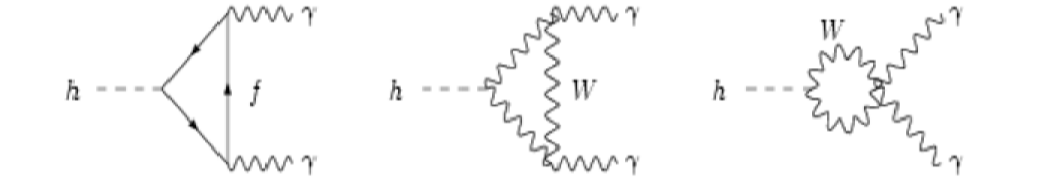
Figure 1: Standard model Feynman graphs contributing to the process $h\to\gamma\gamma$ at the lowest order.

Figure 2: Additional contribution to $h\to\gamma\gamma$ due to the chargino loops in split SUSY.

The colour factor $N_{c}^{f}$ equals 3 for quarks and 1 for leptons. One has $C_{W}=C_{f}=1$, while the chargino coupling is given by,

$$C_{\widetilde{\chi}^{\pm}}=2~{}(S_{ii}~{}\tilde{g_{u}}/g+Q_{ii}~{}\tilde{g_{d}}/g)$$

with $S_{ij}=U_{i1}V_{j2}/\sqrt{2}$ and $Q_{ij}=U_{i2}V_{j1}/\sqrt{2}$. The matrices $\bf{U}$ and $\bf{V}$ diagonalize the chargino mass matrix. In our case $i=1$ and 2 yield the two physical charginos in the loops.

One has to remember that the seed parameters corresponding to split SUSY and MSSM are fixed at the SUSY breaking scale $m_{S}$ and that those featuring in the above expressions are the results of evolution down to the EW scale ($m_{W}$) through renormalization group (RG) equations [1, 2]. However, their low-energy values themselves can be used in the present analysis, without any further reference. We have also assumed gaugino unification, having the low-energy SU(2) gaugino mass $M_{2}$ as an independent parameter. Thus the basic parameters for us are (in addition to those of the standard model) the Higgs mass $m_{h}$ and the SUSY parameters $M_{2}$, $\mu$ (the Higgsino mass) and $tan\beta$ . The latter, not having anything to do with low-energy couplings of the Higgs, can easily evade the bound of $\simeq 2$ obtained from on the measurements of Higgs mass at the Large Electron-Positron (LEP) collider [19]. However, since $\tan\beta$ governs the high-scale Lagrangian and therefore the boundary conditions for the spectrum at the scale $m_{S}$, bounds of the order of 0.5 on its value have been derived from considerations such as the infrared fixed point for the top quark mass [2, 20]. It may be noted that a similar lower bound of about 1.2 can be given on $\tan\beta$ in the MSSM, but it is overridden by the experimental limit. The remaining split SUSY parameters have also been restricted by the lower bound of about 103.5 GeV on the chargino mass [21].

The rate for the inclusive process

$$pp\rightarrow h~{}+~{}X\longrightarrow\gamma\gamma$$

(where Higgs production takes place via gluon fusion) can be expressed in the leading order as

$$R~{}=~{}\frac{\pi^{2}}{8m_{h}s}\frac{\Gamma_{h\rightarrow 2g}\Gamma_{h\rightarrow 2\gamma}}{\Gamma_{tot}}\int^{1}_{\tau}{d\zeta\frac{1}{\zeta}g\left(\zeta,m^{2}_{h}\right)~{}g\left(\frac{\tau}{\zeta},m^{2}_{h}\right)}$$ (13)

where  $\tau=\frac{m^{2}_{h}}{S}$ and $g\left(\zeta,m^{2}_{h}\right)$ is the gluon distribution function evaluated at $Q^{2}~{}=~{}m^{2}_{h}$ and parton momentum fraction $\zeta$. $\Gamma_{h\rightarrow 2\gamma}$ and $\Gamma_{tot}$ stand respectively for the diphoton and total decay widths of the Higgs. The lowest order estimate given above is further multiplied by the appropriate K-factors to obtain the next-to-next leading order (NNLO) predictions in QCD. While the computation of the rate is straightforward, we realise that the various quantities used are beset with theoretical as well as experimental uncertainties [22]. We undertake an analysis of these uncertainties in the next section.

4 Numerical estimate: uncertainties

As has already been stated in the previous section, the rate for diphoton production through real Higgs at LHC is given by

$$R~{}=~{}\sigma(pp\rightarrow h)\times B~{}=~{}\sigma(pp\rightarrow h){\frac{\Gamma(h\rightarrow\gamma\gamma)}{\Gamma_{tot}}}$$ (14)

We have performed a parton-level Monte Carlo calculation for the production cross-section, using the MRS [23] parton distribution functions and multiplied the results with the corresponding NNLO K-factors [24, 25]. It may be noted that NNLO K-factors are not yet available for most other parameterizations. In estimating the statistical uncertainties in the experimental value [26], MRS (at leading order) distributions have been used by the CMS group while ATLAS uses CTEQ distributions. We have obtained the aforesaid uncertainty by taking the estimate based on MRS and multiplying the corresponding event rate by the NNLO K-factor for MRS. It may also be mentioned that the difference between the NLO estimates of Higgs production using the MRS and CTEQ parameterizations is rather small ($\mathrel{\mathchoice{\lower 1.72218pt\vbox{\halign{$\m@th\displaystyle\hfil#\hfil$\cr<\crcr\sim\crcr}}}{\lower 1.72218pt\vbox{\halign{$\m@th\textstyle\hfil#\hfil$\cr<\crcr\sim\crcr}}}{\lower 1.72218pt\vbox{\halign{$\m@th\scriptstyle\hfil#\hfil$\cr<\crcr\sim\crcr}}}{\lower 1.72218pt\vbox{\halign{$\m@th\scriptscriptstyle\hfil#\hfil$\cr<\crcr\sim\crcr}}}}2\%$), according to recent studies [24]. Therefore, it is expected that the NNLO estimate of uncertainties (where there is scope of further evolution in any case) used by us will ultimately converge to even better agreement with other parameterizations and will not introduce any serious inaccuracy in our conclusions. The programme HDECAY3.0 [27], including $\mathcal{O}(\alpha_{s}^{2})$ contributions, has been used for Higgs decay computations .

The number of two-photon events seen is given by $\cal{L}R$ where $\cal{L}$ is the integrated luminosity. $\cal{L}$ is expected to be known at the LHC to within 2 %. We include this uncertainty in our calculation, although it has a rather small effect on our conclusions.

In order to estimate the total uncertainty in $R$, one has to first obtain the spread in theoretically predicted value in the standard model due to the uncertainty in the various parameters used. In addition, however, there is an uncertainty in the experimental values; although the actual level of this will be known only after the LHC run begins, the anticipated statistical spread in the measured value can be estimated through simulations. These two uncertainties, combined in quadrature, are indicative of the difference with central value of the standard model prediction which is required to establish any non-standard effect at any given confidence level. We have performed such an exercise, taking the standard model calculation and that with standard model + chargino contributions.

Parameter	Central Value	Present Uncertainty	LHC Uncertainty(projected)
$m_{h}$	$120-150$	$-$	$0.2$
$m_{W}$	$80.425$	$.034$	$.015$
$m_{t}$	$172.7$	$2.9$	$1.5$
$m_{b}$	$4.62$	$.15$	$-$
$m_{c}$	$1.42$	$.1$	$-$
$m_{\tau}$	$1.777$	$.0003$	$-$
$\alpha_{s}$	$0.1187$	$0.002$	$-$

Table 1: Current and projected uncertainties (at LHC) in the values of various parameters. All the masses are given in $GeV$. The values are extracted from refs [30, 31, 32]

Thus the total uncertainty in $R$ can be expressed as

$${\left(\frac{\delta R}{R}\right)}^{2}~{}=~{}{\left(\frac{\delta R}{R}\right)}_{\it th}^{2}~{}+~{}{\left(\frac{\delta R}{R}\right)}_{\it exp}^{2}$$ (15)

where the theoretical component can be further broken up as

$${\left(\frac{\delta R}{R}\right)}_{\it th}^{2}~{}=~{}\frac{1}{R^{2}}\sum_{i}{\sigma^{2}_{R_{i}}}$$ (16)

where $\sigma_{R_{i}}$ stands for the spread in the prediction of R due to uncertainty in the i^th parameter relevant for the calculation. The sum runs over $m_{h}$, $m_{W}$, $m_{t}$, $m_{b}$, $m_{\tau}$ and $m_{c}$, in addition to the uncertainty in the strong coupling $\alpha_{s}$. The spread in the predicted value is predicted in each case by random generation of values for each parameter (taken to vary one at a time) within the allowed range. Thus we obtain $\frac{1}{R^{2}}{\sigma^{2}_{R_{i}}}$ corresponding to each parameter. One has to further include QCD uncertainties arising via parameterization dependence of the parton distribution functions (PDF) and the renormalisation scale. Although NNLO calculation reduced such uncertainties, the net spread in the prediction due to them could be as large as $\sim 15$ % [24, 25, 28, 29] in the Higgs mass range $120-150$ GeV. The levels of uncertainties in the various parameters, are presented in Table 1. In that table we have given the uncertainties, wherever they are available, from recent and current experiments like the LEP and the Tevatron. In addition, whatever improved measurement, leading to smaller errors (in, say, $m_{t}$ or $m_{W}$) are expected after the initial run of the LHC are also separately incorporated in the table . We have used the estimates corresponding to LHC wherever they are available. In our calculation, we have used two values of the combined uncertainty from PDF and scale-dependence, namely, 15% and 10%, the latter with a view to likely improvement using data at the LHC. This uncertainty is over and above the uncertainty in $\alpha_{s}$ due to the error in measurement of its boundary value at $m_{Z}$. Table 2 contains the finally predicted values of ${\left(\frac{\delta R}{R}\right)}$, for the two values of the Higgs boson mass.

$R_{\it exp}$ includes statistical uncertainties, as estimated in detector simulations with a luminosity of 100 $fb^{-1}$ [26]. As has been already mentioned, we have obtained benchmark values of this quantity using the results for CMS presented in ref [26] for MRS distributions at the lowest order, and appropriately improving them with the NNLO K-factors available in the literature. The resulting predictions for statistical error are $8.1\%$ for $m_{h}=130$ GeV, $8.6\%$ for $m_{h}=140$ GeV and $11.3\%$ for $m_{h}=150$ GeV.

Total Uncertainty in Standard Model Rate
Higgs mass (GeV)	PDF + Scale Uncertainty$=15\%$	PDF + Scale Uncertainty$=10\%$
$130$	$18.5\%$	$14.7\%$
$140$	$18.3\%$	$14.4\%$
$150$	$19.4\%$	$15.8\%$

Table 2: Expected total uncertainties in standard model rate at LHC. Entries in the second (third) column corresponds to total uncertainty from parton distributions and renormalization scale being equal to $15\%$ ($10\%$).

Thus one is able to obtain the net ($1\sigma$ level) uncertainties in the standard model. Next, the split SUSY contributions via chargino-induced diagrams are calculated and added to the standard model amplitude. The observable decay rate obtained therefrom is compared with that predicted in the standard model taking the uncertainty into account at various confidence levels. Thus one is able to decide whether the chargino contributions to the diphoton rate are discernible from the standard model contributions at a given confidence level for a particular combination of split SUSY parameters.

$m_{h}$  (GeV)	$tan\beta$	$m_{S}$  (GeV)
$130$	$1.0$	$1\times 10^{5}-1\times 10^{6}$
	$1.5$	$0.7\times 10^{5}-5\times 10^{5}$
$140$	$1.0$	$3\times 10^{7}-6\times 10^{8}$
	$1.5$	$2\times 10^{6}-4\times 10^{7}$
$150$	$1.2$	$7\times 10^{12}-9\times 10^{12}$
	$1.5$	$0.9\times 10^{12}-2\times 10^{12}$

Table 3: Allowed ranges of $m_{S}$, corresponding to the three low-scale Higgs masses used here.

The realistic estimate requires subjecting the predictions to some experimental cuts aimed at maximizing the signal-to-background ratio as well as focusing on kinematic regions of optimal observability. We incorporate the effects of such cuts with the help of an efficiency factor which, on explicit calculation in representative cases, turns out to be approximately 50%. The only assumptions required are that the percentage error due to various parameters are the same for uncut rates as those calculated with cuts, and that the standard and split SUSY contributions suffer the same reduction due to cuts. We have checked that this holds true so long as the kinematic region is not drastically curtailed by the cuts.

Before we end this section, it should be noted that the various uncertainties quoted above are only benchmark values. The precise levels of these uncertainties will be known after the LHC comes into operation.

5 Numerical estimate: discussions

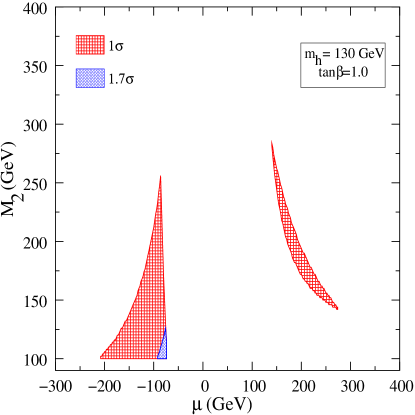
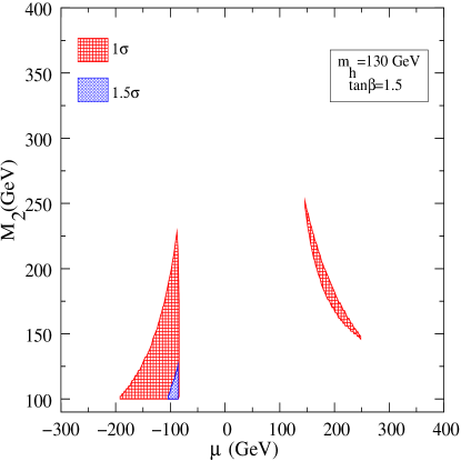
Figure 3: Contour plots for $m_{h}=130$ GeV assuming PDF + scale uncertainty $=15\%$.

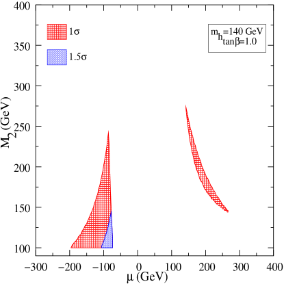
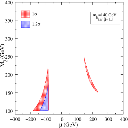
Figure 4: Contour plots for $m_{h}=140$ GeV assuming PDF + scale uncertainty $=15\%$.

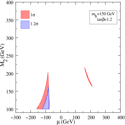
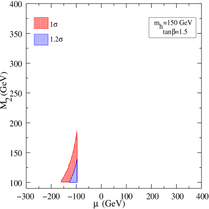
Figure 5: Contour plots for $m_{h}=150$ GeV assuming PDF + scale uncertainty $=15\%$.

Our purpose is to see at what confidence levels one can distinguish the split SUSY effects on $h\longrightarrow\gamma\gamma$. With this in view, we have presented, in figures 3 - 8, sets of contour plots in the $M_{2}$-$\mu$ plane with different values of $\tan\beta$, for $m_{h}=130$ GeV, $140$ GeV and $150$ GeV.

Since the low-scale parameters in this scenario originate in specific boundary conditions at the SUSY breaking scale $(m_{S})$, one needs to emphasize that not all such parameters are consistent. In general, the value of $m_{h}$ is determined (modulo the uncertainties due to parameters such as $\alpha_{s}$ and top quark mass) once $tan\beta$ and $m_{S}$ are fixed. In this study, we are essentially interested in the low energy parameters which can make a difference from the standard model estimate. Therefore, for each $tan\beta$ used, we have found the scale $(m_{S})$, so as to reproduce the Higgs mass used in the corresponding case. Such allowed ranges of $m_{S}$ are presented in the Table 3. In obtaining these values, the procedure adopted is as follows. Using a given value of $tan\beta$ as boundary conditions at $m_{S}$, and values of gauge couplings at the EW scale, one solves the renormalisation group equations, going through an iterative process till convergence is achieved. Then the quartic coupling $\lambda$ is evolved down to the EW scale, using $tan\beta$ as well as the gauge couplings at $m_{S}$ to determine its boundary value (see equation 3), whereby the Higgs mass $(m_{h})$ is obtained. For each value of $m_{h}$ used in our numerical study, we have the value of $m_{S}$ which achieves that particluar $m_{h}$, for a given $tan\beta$. In this way we find that $m_{h}=130-150$ GeV is a ’reasonable’ range, for which, with the given value of $tan\beta$, $m_{S}$ can be $\mathrel{\mathchoice{\lower 1.72218pt\vbox{\halign{$\m@th\displaystyle\hfil#\hfil$\cr<\crcr\sim\crcr}}}{\lower 1.72218pt\vbox{\halign{$\m@th\textstyle\hfil#\hfil$\cr<\crcr\sim\crcr}}}{\lower 1.72218pt\vbox{\halign{$\m@th\scriptstyle\hfil#\hfil$\cr<\crcr\sim\crcr}}}{\lower 1.72218pt\vbox{\halign{$\m@th\scriptscriptstyle\hfil#\hfil$\cr<\crcr\sim\crcr}}}}10^{13}$ GeV and at the same time not too close to the TeV scale. We have deliberately avoided imposing further constraints on $m_{S}$ in this phenomenological study. For $m_{h}=120$ GeV or less, $m_{S}$ tend to violate the aforesaid condition; therefore, we have started from $m_{h}=130$ GeV.

The quantities ${\tilde{g_{u}}}/{\tilde{g_{d}}}$ and ${\tilde{g^{\prime}_{u}}}/{\tilde{g^{\prime}_{d}}}$ are both equal to $tan\beta$ at the scale $m_{S}$, and thus their values at low scale are obtained through running. Such values are used in the chargino mass matrix and Higgs-chargino coupling.

In the first three graphs, the total uncertainty arising from PDF as well as the renormalisation scale has been taken to be 15%. The results where this uncertainty is 10%, corresponding to a projected convergence of different PDF parameterizations as well as improvement over the current NNLO results, are shown in figures 6 - 8. The allowed regions represented by the contours are also subjected to the restriction that the mass of the lighter chargino be above the current experimental limit of 103.5 GeV.

The results in all the above cases show that the distinguishability with the standard model effect is maximum for such values of $\mu$ and $M_{2}$ which leads to the lowest possible chargino masses contributing in the loops. For negative $\mu$, lower values of $|\mu|$ are allowed by the above constraints; hence an asymmetry about $\mu=0$ is seen. The dependence on $\tan\beta$ is also substantial. The maximum departure from the standard model contribution occurs for $\tan\beta=1$. This is because the Higgs-chargino-chargino coupling is maximum when the charginos have equal admixture of the Wino and Higgsino components. When no CP - violating phase in the mixing is assumed, there is also a symmetry of the coupling under $\tan\beta\rightarrow\cot\beta$.

It is clear from the contours that the general level of expected distinguishability of the split SUSY contributions is quite low. This is primarily due to the uncertainty of “PDF + renormalisation scale”. However, even if this uncertainty is brought down from 15% to 10%, one notices that one is barely allowed a small area of the parameter space for $\tan\beta~{}\simeq~{}1$, where predicted effects are about $2\sigma$; otherwise the results are even less optimistic. The distinguishability goes down considerably for high values of $\tan\beta$. The other important source of uncertainty is in the b-quark mass (calculated at the scale $m_{h}$, with the boundary condition that the pole mass is $4.62$ GeV) which affects the total width for $h\longrightarrow b\bar{b}$. The results look even less optimistic if one remembers that searches in, for example, the trilepton channel at the LHC are likely to raise the experimental lower limit of the chargino mass, unless the lighter chargino lies just beyond the LEP limit. Under such circumstances, the confidence level for distinguishing the chargino effects in the diphoton signal will be further diminished, and the $2\sigma$ region will be obliterated in all likelihood.

6 Summary and conclusions

We have undertaken a thorough analysis of the split SUSY parameter space to see if the channel $h\longrightarrow\gamma\gamma$ can allow one to isolate the contributions from chargino-induced loops. In the case of split SUSY, this is supposedly the only channel where the sole surviving Higgs at the electroweak symmetry breaking scale can reveal any difference with respect to its counterpart in the standard model. Although the chargino contribution has been already calculated, our analysis, with all uncertainties duly incorporated in the production as well as decay level, confirms that the measurable effects are very small in all over the allowed parameter space. It is going to be very difficult to achieve a $2\sigma$ difference with respect to the standard model predictions, and that too for the value of $\tan\beta$ in the neighbourhood of 1. Thus it appears to us that the only way to uncover split SUSY is to carry out an exhaustive search for the entire superparticle spectrum at the LHC, unless some other ingenious method can be devised to see the difference in Higgs couplings with the SUSY fermions.

Acknowledgment: We thank Anindya Datta, Aseshkrishna Datta, G.F. Giudice, A. Romanino, V. Ravindran and Sourov Roy for useful comments.

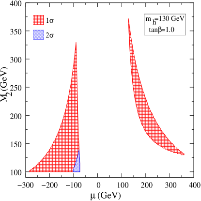
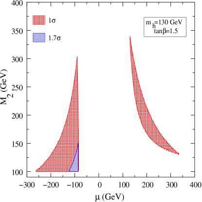
Figure 6: Contour plots for $m_{h}=130$ GeV assuming PDF + scale uncertainty $=10\%$.

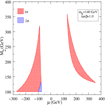
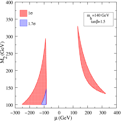
Figure 7: Contour plots for $m_{h}=140$ GeV assuming PDF + scale uncertainty $=10\%$.

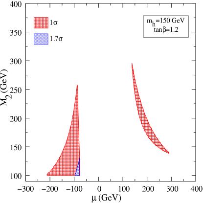
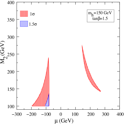
Figure 8: Contour plots for $m_{h}=150$ GeV assuming PDF + scale uncertainty $=10\%$.

References

- [1] N. Arkani-Hamed and S. Dimopoulos, JHEP 0506, 073 (2005) [arXiv:hep-th/0405159].
- [2] G. F. Giudice and A. Romanino, Nucl. Phys. B 699, 65 (2004) [Erratum-ibid. B 706, 65 (2005)] [arXiv:hep-ph/0406088].
- [3] M. A. Diaz and P. F. Perez, J. Phys. G 31, 563 (2005) [arXiv:hep-ph/0412066].
- [4] A. Arvanitaki, C. Davis, P. W. Graham and J. G. Wacker, Phys. Rev. D 70, 117703 (2004) [arXiv:hep-ph/0406034]; R. Mahbubani, [arXiv:hep-ph/0408096].
- [5] M. Drees, [arXiv:hep-ph/0501106].
- [6] N. Arkani-Hamed, S. Dimopoulos, G. F. Giudice and A. Romanino, Nucl. Phys. B 709, 3 (2005) [arXiv:hep-ph/0409232].
- [7] C. Kokorelis, [arXiv:hep-th/0406258]; B. Mukhopadhyaya and S. SenGupta, Phys. Rev. D 71, 035004 (2005) [arXiv:hep-th/0407225]; U. Sarkar, Phys. Rev. D 72, 035002 (2005) [arXiv:hep-ph/0410104]; I. Antoniadis and S. Dimopoulos, Nucl. Phys. B 715, 120 (2005) [arXiv:hep-th/0411032]; J. D. Wells, Phys. Rev. D 71, 015013 (2005) [arXiv:hep-ph/0411041]; B. Bajc and G. Senjanovic, Phys. Lett. B 610, 80 (2005) [arXiv:hep-ph/0411193]; B. Kors and P. Nath, Nucl. Phys. B 711, 112 (2005) [arXiv:hep-th/0411201]; K. S. Babu, T. Enkhbat and B. Mukhopadhyaya, Nucl. Phys. B 720, 47 (2005) [arXiv:hep-ph/0501079]; K. Cheung and C. W. Chiang, Phys. Rev. D 71, 095003 (2005) [arXiv:hep-ph/0501265]; N. Haba and N. Okada, [arXiv:hep-ph/0502213]; B. Dutta and Y. Mimura, [arXiv:hep-ph/0503052]; B. Mukhopadhyaya and S. SenGupta, [arXiv:hep-ph/0503167]; I. Antoniadis, A. Delgado, K. Benakli, M. Quiros and M. Tuckmantel, [arXiv:hep-ph/0507192].
- [8] W. Kilian, T. Plehn, P. Richardson and E. Schmidt, Eur. Phys. J. C 39, 229 (2005) [arXiv:hep-ph/0408088]; D. A. Demir, [arXiv:hep-ph/0410056]; R. Allahverdi, A. Jokinen and A. Mazumdar, Phys. Rev. D 71, 043505 (2005) [arXiv:hep-ph/0410169]; E. J. Chun and S. C. Park, JHEP 0501, 009 (2005) [arXiv:hep-ph/0410242]; M. Beccaria, F. M. Renard and C. Verzegnassi, Phys. Rev. D 71, 093008 (2005) [arXiv:hep-ph/0412257]; J. Cao and J. M. Yang, Phys. Rev. D 71, 111701 (2005) [arXiv:hep-ph/0412315]; S. Kasuya and F. Takahashi, Phys. Rev. D 71, 121303 (2005) [arXiv:hep-ph/0501240]; N. G. Deshpande and J. Jiang, Phys. Lett. B 615, 111 (2005) [arXiv:hep-ph/0503116]; A. Ibarra, Phys. Lett. B 620, 164 (2005) [arXiv:hep-ph/0503160]. J. Guasch and S. Penaranda, [arXiv:hep-ph/0508241].
- [9] J. L. Hewett, B. Lillie, M. Masip and T. G. Rizzo, JHEP 0409, 070 (2004) [arXiv:hep-ph/0408248]; K. Cheung and W. Y. Keung, Phys. Rev. D 71, 015015 (2005) [arXiv:hep-ph/0408335]; M. Toharia and J. D. Wells, [arXiv:hep-ph/0503175]; A. Arvanitaki, C. Davis, P. W. Graham, A. Pierce and J. G. Wacker, [arXiv:hep-ph/0504210]; J. G. Gonzalez, S. Reucroft and J. Swain, [arXiv:hep-ph/0504260]; P. Gambino, G. F. Giudice and P. Slavich, [arXiv:hep-ph/0506214]; A. Arvanitaki, S. Dimopoulos, A. Pierce, S. Rajendran and J. Wacker, [arXiv:hep-ph/0506242]; F. Wang, W. Wang and J. M. Yang, [arXiv:hep-ph/0507172].
- [10] C. H. Chen and C. Q. Geng, [arXiv:hep-ph/0501001]; C. H. Chen and C. Q. Geng, [arXiv:hep-ph/0502246].
- [11] S. h. Zhu, Phys. Lett. B 604, 207 (2004) [arXiv:hep-ph/0407072]; S. P. Martin, K. Tobe and J. D. Wells, Phys. Rev. D 71, 073014 (2005) [arXiv:hep-ph/0412424]; K. Cheung and J. Song, [arXiv:hep-ph/0507113].
- [12] A. Pierce, Phys. Rev. D70, 075006 (2004) [arXiv:hep-ph/0406144]; L. Anchordoqui, H. Goldberg and C. Nunez, Phys. Rev. D 71, 065014 (2005) [arXiv:hep-ph/0408284]; A. Arvanitaki and P. W. Graham, Phys. Rev. D 72, 055010 (2005) [arXiv:hep-ph/0411376]; A. Masiero, S. Profumo and P. Ullio, Nucl. Phys. B 712, 86 (2005) [arXiv:hep-ph/0412058].
- [13] D. Chang, W. F. Chang and W. Y. Keung, Phys. Rev. D 71, 076006 (2005) [arXiv:hep-ph/0503055]; G. F. Giudice and A. Romanino, [arXiv:hep-ph/0510197].
- [14] S. K. Gupta, P. Konar and B. Mukhopadhyaya, Phys. Lett. B 606, 384 (2005) [arXiv:hep-ph/0408296].
- [15] ATLAS Collaboration, ATLAS Detector and Physics Performance Technical Design Report, report CERN-LHCC-99-15 (1999).
- [16] CMS Collaboration, CMS, the Compact Muon Solenoid: Technical proposal, report CERN-LHCC-94-38 (1994).
- [17] H. Zheng and D. Wu, Phys. Rev. D 42, 3760 (1990); A. Djouadi, M. Spira, J. J. van der Bij and P. M. Zerwas, Phys. Lett. B 257, 187 (1991); S. Dawson and R. P. Kauffman, Phys. Rev. D 47, 1264 (1993); K. Melnikov and O. I. Yakovlev, Phys. Lett. B 312, 179 (1993) [arXiv:hep-ph/9302281]; A. Djouadi, M. Spira and P. M. Zerwas, Phys. Lett. B 311, 255 (1993) [arXiv:hep-ph/9305335]; M. Inoue, R. Najima, T. Oka and J. Saito, Mod. Phys. Lett. A 9, 1189 (1994); Y. Liao and X. y. Li, Phys. Lett. B 396, 225 (1997) [arXiv:hep-ph/9605310]; M. Steinhauser, [arXiv:hep-ph/9612395]; A. Djouadi, P. Gambino and B. A. Kniehl, Nucl. Phys. B 523, 17 (1998) [arXiv:hep-ph/9712330]; J. Fleischer, O. V. Tarasov and V. O. Tarasov, Phys. Lett. B 584, 294 (2004) [arXiv:hep-ph/0401090].
- [18] U. Aglietti, R. Bonciani, G. Degrassi and A. Vicini, Phys. Lett. B 595, 432 (2004) [arXiv:hep-ph/0404071]; G. Degrassi and F. Maltoni, [arXiv:hep-ph/0504137].
- [19] The ALEPH, DELPHI, L3 and OPAL Colaborations, and the LEP Higgs Working Group, ”Search for the Standard Model Higgs Boson at LEP” , LEP Higgs WG Note 2001-03, July 2001.
- [20] K. Huitu, J. Laamanen, P. Roy and S. Roy, Phys. Rev. D 72, 055002 (2005) [arXiv:hep-ph/0502052];
- [21] ALEPH Collaboration (A Heiser et al.) Phys. Lett. B533 (2002) 223.
- [22] M. Duhrssen, S. Heinemeyer, H. Logan, D. Rainwater, G. Weiglein and D. Zeppenfeld, Phys. Rev. D 70, 113009 (2004) [arXiv:hep-ph/0406323].
- [23] A. D. Martin, R. G. Roberts, W. J. Stirling and R. S. Thorne, Phys. Lett. B 531, 216 (2002) [arXiv:hep-ph/0201127].
- [24] V. Ravindran, J. Smith and W. L. van Neerven, Nucl. Phys. B 665, 325 (2003) [arXiv:hep-ph/0302135].
- [25] C. Anastasiou and K. Melnikov, Nucl. Phys. B 646, 220 (2002) [arXiv:hep-ph/0207004]; R. V. Harlander and W. B. Kilgore, Phys. Rev. Lett. 88, 201801 (2002) [arXiv:hep-ph/0201206].
- [26] D. Zeppenfeld, R. Kinnunen, A. Nikitenko and E. Richter-Was, Phys. Rev. D 62, 013009 (2000) [arXiv:hep-ph/0002036].
- [27] A. Djouadi, J. Kalinowski and M. Spira, Comput. Phys. Commun. 108, 56 (1998) [arXiv:hep-ph/9704448].
- [28] A. Belyaev, J. Pumplin, W. K. Tung and C. P. Yuan, [arXiv:hep-ph/0508222].
- [29] A. Cafarella, C. Coriano’, M. Guzzi and J. Smith, [arXiv:hep-ph/0510179].
- [30] S. Eidelman et al. [Particle Data Group], Phys. Lett. B 592, 1 (2004).
- [31] [CDF Collaboration], [arXiv:hep-ex/0507091].
- [32] S. Heinemeyer, W. Hollik and G. Weiglein, [arXiv:hep-ph/0412214].