QCD sum rules for the anti-charmed pentaquark

Abstract

We present a QCD sum rule analysis for the anti-charmed pentaquark state with and without strangeness. While the sum rules for most of the currents are either non-convergent or dominated by the $DN$ continuum, the one for the non-strange pentaquark current composed of two diquarks and an antiquark, is convergent and has a structure consistent with a positive parity pentaquark state after subtracting out the $DN$ continuum contribution. Arguments are presented on the similarity between the result of the present analysis and that based on the constituent quark models, which predict a more stable pentaquark states when the antiquark is heavy.

I Introduction

The observation of the $\Theta^{+}$ by the LEPS collaborationLeps03 and its subsequent confirmation have brought a lot of excitements in the field of hadronic physicsOTHERS . On the other hand, there are increasing number of experiments reporting negative results. In particular, the latest experiments at JLABEsmith find no signal from the photoproduction process on a deuteron nor on a proton target, from which the $\Theta^{+}$ was observed earlier by the SAPHIR collaboration with lower statistics. Although the present experimental results are quite confusing and frustratinghicks , one can not afford to give up further refined experimental search, because if a pentaquark is found, it will provide a major and unique testing ground for QCD dynamics at low energy.

Another multiplet to search for as possible pentaquark states are those with one heavy antiquark. The H1 collaboration at HERA has recently reported on the finding of an anti-charmed pentaquark $\Theta_{c}(3099)$ from the $D^{*}p$ invariance mass spectrumAktas:2004qf . Unfortunately other experiments could not confirm the findingLitvintsev:2004yw ; Karshon:2004kt ; Link:2005ti . While the experimental search for the heavy pentaquark is as confusing as that for the light, theoretically, the heavy and light pentaquarks stand on quite different grounds. Cohen showed that the original prediction for the mass of the $\Theta^{+}$ based on the SU(3) Skyrme modelDPP97 is not valid because collective quantization of the model for the anti-decuplet states is inconsistent in the large $N_{c}$ limitCohen:2003yi . In contrast, many theories consistently predicted a stable heavy pentaquark state. The pentaquark with one heavy anti-quark was first studied in Ref. GSR87 ; Lip87 in a quark model with color spin interaction. Then it has been studied in quark models with flavor spin interactionStan98 and Skyrme models RS93 ; OPM94 , and with the recent experiments, attracted renewed interests CBSC ; P04dw ; Stewart:2004pd , some of which were motivated by the diquark-diquarkJW03 and diquark-triquarkKL03a picture. Such states also appear naturally in a coupled channel approachlutz , and in the combined large $N_{c}$ and heavy quark limit of QCDCohen:2005bx . If the heavy pentaquark state is stable against strong decay, as was predicted in the $D$ meson bound solition modelsRS93 , it could only be observed from the weak decay of the virtual $D$ meson. From a constituent quark model picture based on the color spin interaction Jaffe77 , one expects a strong diquark correlation, from which one could have a stable diquark-diquark-antiquarkJW03 or diquark triquarkLip87 structure. The question is whether such strong diquark structure will survive other non-perturbative QCD dynamics in a multiquark environment and produce a stable pentaquark state. Such questions are being intensively pursued in quark model approachesHiyama:2005cf ; Stancu:2005jv ; Maltman:2004qe . In particular, an important question at hand is whether the net attraction from the diquark correlations in the pentaquark configuration is stronger than that from the corresponding diquark and additional quark-antiquark correlation present when the pentaquark separates into a nucleon and a meson state. Since the correlation are inversely proportional to the constituent quark masses involved, the attraction is expected to be more effective for pentaquark state with heavy antiquark. Another non-perturbative approach that can be used to answer such question is the QCD sum rule method.

There have been several QCD sum rule calculations for the light pentaquark statesZhu03 ; MNNRL03 ; SDO03 ; Eidemuller:2004ra ; Lee:2004dp ; Eidemuller:2005jm ; Matheus:2004gx . The application to the heavy pentaquarks was performed by two of us in a previous workhung04 , where we used a pentaquark current composed of two diquarks and an antiquark, and found the sum rule to be consistent with a stable positive parity pentaquark state. The similar approach has been applied to the sum rules for $D_{s}(2317)$ Kim05 . In this work, we extend the previous QCD sum rule calculation to investigate the anti-charmed pentaquark state with and without strangeness using two different currents for each case. We find a convergent Operator Product Expansion (OPE) only for the non-strange heavy pentaquark sum rule obtained with an interpolating field composed of two diquarks and one anti-charm quark, that has been previously used by us hung04 . The stability of non-strange heavy pentaquark is consistent with the result based on the quark model with flavor spin interactionStancu:2005jv . We then refine the convergent sum rule by explicitly including the $DN$ two-particle irreducible contribution. The importance of subtracting out such two-particle irreducible contribution has been emphasized in Ref. Kondo05 ; Lee04 ; Kwon05 for the light pentaquark state. In fact, estimating the contribution from the lowest two-particle irreducible contribution is equally important in lattice gauge theory calculations Sasaki03 ; CFKK03 to isolate the signal for the pentaquark state from the low-lying continuum state. We find that for the non-strange heavy pentaquark sum rule, including the $DN$ continuum contribution tends to shift the position of the pentaquark state downwards. Given the negative experimental signatures of the charmed pentaquark states above the threshold, the present result suggests that the anti-charmed pentaquark states might be bound as was predicted in $D$ meson bound soliton models.

This paper is organized as follows. In Section II, we introduce the interpolating field for the $\Theta_{c}$ and discuss the dispersion relations that we will be using. Section III gives the phenomenological side and Section IV gives the OPE side. The QCD sum rules for $\Theta_{c}$ and their analysis are given in Section V.

II QCD sum rules

II.1 Interpolating field for $\bm{\Theta_{c}}$

Let us introduce the following two interpolating field for $\Theta_{c}$,

$$\Theta_{c1} = \epsilon^{abc}(u^{T}_{a}C\gamma_{\mu}u_{b})\gamma_{5}\gamma_{\mu}d_{c}(\bar{c}_{d}i\gamma_{5}d_{d})\ ,$$

$$\Theta_{c2} = \epsilon^{abk}(\epsilon^{aef}u^{T}_{e}C\gamma_{5}d_{f})(\epsilon^{bgh}u^{T}_{g}Cd_{h})C\bar{c}^{T}_{k}\ .$$ (1)

Here the Roman indices $a,b,\dots$ are color indices, $C$ denotes charge conjugation, $T$ transpose. Note that $\Theta_{c1}$ is composed of a nucleon current ($proton$) and a pseudo scalar current ($D$), while $\Theta_{c2}$ is composed of diquark-diquark-antiquark and has been investigated in a previous workhung04 .

For the charmed pentaquark with strangeness, we consider the following two possible currents,

$$\Theta_{cs1} = \epsilon^{abk}(\epsilon^{aef}u^{T}_{e}Cs_{f})(\epsilon^{bgh}u^{T}_{g}Cd_{h})C\bar{c}^{T}_{k}\ ,$$

$$\Theta_{cs2} = \epsilon^{abk}(\epsilon^{aef}u^{T}_{e}C\gamma_{5}s_{f})(\epsilon^{bgh}u^{T}_{g}Cd_{h})C\bar{c}^{T}_{k}\ .$$ (2)

Here, instead of choosing $\Theta_{cs1}$ as a direct product of a nucleon and a $D_{s}$ or a hyperon and a $D$ meson currents as in $\Theta_{c1}$, we choose it to well represent a state having two diquark structure with the same scalar quantum number but with different flavor. Such configuration allows all the five constituent quarks to be in the $s$-wave states, which will have the lowest orbital energy and consequently could be the dominant ground state configurationStewart:2004pd . Moreover, as we will see, $\Theta_{c1}$ couples dominantly to the nucleon and $D$ meson state, suggesting that currents composed of a direct product of a nucleon and a meson currents are not suitable for investigating the properties of the pentaquark state.

Under parity transformation $q^{\prime}(x^{\prime})=\gamma_{0}q(x)$, the $\Theta_{c}$ currents transform as,

$$\Theta_{c1}^{\prime} = -\gamma_{0}\Theta_{c1}\ ,\quad\Theta_{c2}^{\prime}=\gamma_{0}\Theta_{c2}\ ,$$

$$\Theta_{cs1}^{\prime} = -\gamma_{0}\Theta_{cs1}\ ,\quad\Theta_{cs2}^{\prime}=\gamma_{0}\Theta_{cs2}.$$ (3)

II.2 Dispersion relation

The first type of QCD sum rules for the heavy pentaquarks that we will be using are constructed from the following time ordered correlation function,

$$\Pi_{T}(q)=i\int d^{4}xe^{iq\cdot x}\langle 0|T[\Theta_{c}(x),{\bar{\Theta}_{c}}(0)]|0\rangle\ \equiv\Pi_{1}(q^{2})+\ooalign{\hfil/\hfil\crcr$q$}\Pi_{q}(q^{2})\ ,$$ (6)

where $\Theta_{c}$ can be any of the currents in Eq. (1) or in Eq. (2), and $\Pi_{q}$, $\Pi_{1}$ are called the chiral even and chiral odd parts respectively. As can be seen in Eq. (3), the currents are not eigenstates of the parity transformation and can couple to both positive and negative parity states. The spectral densities calculated from the OPE of Eq.(6) are matched to that obtained from the phenomenological assumption in the Borel-weighted dispersion integral,

$$\int^{S_{0}}_{m_{c}^{2}}dq^{2}e^{-q^{2}/M^{2}}W(q^{2}){1\over\pi}{\rm Im}[\Pi_{i}^{\rm phen}(q^{2})-\Pi_{i}^{\rm ope}(q^{2})]=0\ ,\qquad(i=1,q)\ ,$$ (7)

where $M^{2}$ is the Borel mass. Here, higher resonance contributions are subtracted according to the QCD duality assumption, which introduces the continuum threshold $S_{0}$. We have also introduced an additional weight function $W(q^{2})$ for later use.

In this work, we will also work with the “old-fashioned” correlation function, which is defined asSDO03

$$\Pi_{T}(q)=i\int d^{4}xe^{iq\cdot x}\langle 0|\theta(x^{0})\Theta_{c}(x)\bar{\Theta}_{c}(0)|0\rangle\ .$$ (8)

This type of correlation function has been used in projecting out positive and negative parity nucleon states Jido:1996ia . We then divide the imaginary part into the following two parts, which are defined only for $q_{0}>0$,

$$\frac{1}{\pi}{\rm Im}\Pi(q_{0}) = A(q_{0})\gamma^{0}+B(q_{0})\ .$$ (9)

One should note that these can be identified with the imaginary part calculated from Eq.(6),

$$A(q_{0}) = \frac{1}{\pi}{\rm Im}\Pi_{q}(q_{0})q_{0}$$

$$B(q_{0}) = \frac{1}{\pi}{\rm Im}\Pi_{1}(q_{0}),$$ (10)

for $q_{0}>0$.

Now, depending on the parity of the current $\Theta_{c}$ in Eq.(3), one can extract the positive or negative-parity physical state only by either adding or subtracting $A$ and $B$. That is, the spectral density for the positive and negative parity physical states will be as follows,

$$\rho^{\pm}(q_{0})=\bigg{\{}\begin{array}[]{cc}A(q_{0})\mp B(q_{0})&{\rm For}\,\,\,\Theta_{c1},\Theta_{cs1}\\ A(q_{0})\pm B(q_{0})&{\rm For}\,\,\,\Theta_{c2},\Theta_{cs2}\end{array}.$$ (13)

The sum rules are then obtained by again matching the corresponding spectral density from the OPE and phenomenological side,

$$\int^{\infty}_{0}dq_{0}e^{-q_{0}^{2}/M^{2}}[\rho_{\rm phen}^{\pm}(q_{0})-\rho_{\rm ope}^{\pm}(q_{0})]=0\ .$$ (14)

III Phenomenological side

III.1 $\Theta_{c1},\Theta_{cs1}$

For $\Theta_{c1}$ current, the interpolating field couples to a positive parity state as,

$$\langle 0|\Theta_{c1}(x)|\Theta_{c}({\bf p}):P=+\rangle=\lambda_{+,c1}~{}\gamma_{5}U_{\Theta}({\bf p})e^{-ip\cdot x}\ ,$$ (15)

and to a negative parity state as,

$$\langle 0|\Theta_{c1}(x)|\Theta_{c}({\bf p}):P=-\rangle=\lambda_{-,c1}U_{\Theta}({\bf p})e^{-ip\cdot x}\ .$$ (16)

Here, $\lambda_{\pm,c1}$ denotes the coupling strength between the interpolating field and the physical state with the specified parity. Similar relations will hold for $\Theta_{cs1}$. Using these, we obtain the phenomenological side of Eq. (6) separated into chiral even ($\Pi_{q}$) and odd ($\Pi_{1}$) parts, which are defined to be the parts proportional to / $q$ and $1$ respectively.

As was first pointed out in Ref.Kondo05 , the correlation function can also couple to the $DN$ continuum state, whose threshold could be lower than the expected $\Theta_{c}$ mass. Its phenomenological contribution can be estimated by using,

$$\langle 0|\Theta_{c1}|DN({\bf p})\rangle=i\lambda_{DN,c1}U_{N}({\bf p})\ .$$ (17)

Combining these two contributions, we find

$$\Pi^{\rm phen}_{T,c1}(q)=-|\lambda_{\pm,c1}|^{2}~{}{\ooalign{\hfil/\hfil\crcr$q$}\mp m_{\Theta}\over q^{2}-m^{2}_{\Theta}}-i|\lambda_{DN,c1}|^{2}\int d^{4}p\frac{(\ooalign{\hfil/\hfil\crcr$p$}+m_{N})}{p^{2}-m_{N}^{2}}\frac{1}{(p-q)^{2}-m_{D}^{2}}+\cdot\cdot\cdot,$$ (22)

where the minus (plus) sign in front of $m_{\Theta}$ is for positive (negative) parity. The dots denote higher resonance contributions that should be parameterized according to QCD duality. It should be noted however that higher resonances with different parities contribute differently to the chiral-even and chiral odd parts Jin:1997pb . Thus, $\Pi^{\rm phen}_{q}$ and $\Pi^{\rm phen}_{1}$ constitute separate sum rules. For $\Theta_{cs1}$, the $D$ meson should be replaced by the $D_{s}$ meson.

The corresponding spectral density for the pole and $DN$ contributions are given respectively by

$${1\over\pi}{\rm Im}\Pi^{\rm pole}_{T,c1}(q) = \ooalign{\hfil/\hfil\crcr$q$}|\lambda_{\pm,c1}|^{2}\delta(q^{2}-m^{2}_{\Theta})\mp m_{\Theta}|\lambda_{\pm,c1}|^{2}\delta(q^{2}-m^{2}_{\Theta}),$$ (25)

$${1\over\pi}{\rm Im}\Pi^{\rm DN}_{T,c1}(q) = \ooalign{\hfil/\hfil\crcr$q$}|\lambda_{DN,c1}|^{2}\frac{q^{2}+m_{N}^{2}-m_{D}^{2}}{32\,\pi^{2}\,q^{4}}\sqrt{q^{4}-2q^{2}(m_{N}^{2}+m_{D}^{2})+(m_{N}^{2}-m_{D}^{2})^{2}}$$ (29)

$$+|\lambda_{DN,c1}|^{2}\frac{2m_{N}}{32\,\pi^{2}\,q^{2}}\sqrt{q^{4}-2q^{2}(m_{N}^{2}+m_{D}^{2})+(m_{N}^{2}-m_{D}^{2})^{2}}.$$

We notice that the chiral-odd part has opposite sign depending on the parity while the chiral even part has positive-definite coefficient.

III.2 $\Theta_{c2},\Theta_{cs2}$

As can be seen in Eq.(3), $\Theta_{c2}$ transforms differently compared to $\Theta_{c1}$ under parity. Thus, the couplings to the interpolating field are

$$\langle 0|\Theta_{c2}(x)|\Theta_{c}({\bf p}):P=+\rangle = \lambda_{+,c2}U_{\Theta}({\bf p})e^{-ip\cdot x}\ ,$$

$$\langle 0|\Theta_{c2}(x)|\Theta_{c}({\bf p}):P=-\rangle = \lambda_{-,c2}~{}\gamma_{5}U_{\Theta}({\bf p})e^{-ip\cdot x}\ .$$ (30)

Similarly, the coupling to the $DN$ continuum state changes as follows,

$$\langle 0|\Theta_{c2}|DN({\bf p})\rangle=\lambda_{DN,c2}\gamma_{5}U_{N}({\bf p}).$$ (31)

Combining these changes, we find,

$$\Pi^{\rm phen}_{T,c2}(q)=-|\lambda_{\pm,c2}|^{2}~{}{\ooalign{\hfil/\hfil\crcr$q$}\pm m_{\Theta}\over q^{2}-m^{2}_{\Theta}}+i|\lambda_{DN,c2}|^{2}\int d^{4}p\frac{\gamma_{5}(\ooalign{\hfil/\hfil\crcr$p$}+m_{N})\gamma_{5}}{p^{2}-m_{N}^{2}}\frac{1}{(p-q)^{2}-m_{D}^{2}}+\cdot\cdot\cdot.$$ (36)

Consequently, the spectral densities are,

$${1\over\pi}{\rm Im}\Pi^{\rm pole}_{T,c2}(q) = \ooalign{\hfil/\hfil\crcr$q$}|\lambda_{\pm,c2}|^{2}\delta(q^{2}-m^{2}_{\Theta})\pm m_{\Theta}|\lambda_{\pm,c2}|^{2}\delta(q^{2}-m^{2}_{\Theta}),$$ (39)

$${1\over\pi}{\rm Im}\Pi^{\rm DN}_{T,c2}(q) = \ooalign{\hfil/\hfil\crcr$q$}|\lambda_{DN,c2}|^{2}\frac{q^{2}+m_{N}^{2}-m_{D}^{2}}{32\,\pi^{2}\,q^{4}}\sqrt{q^{4}-2q^{2}(m_{N}^{2}+m_{D}^{2})+(m_{N}^{2}-m_{D}^{2})^{2}}$$ (43)

$$-|\lambda_{DN,c2}|^{2}\frac{2m_{N}}{32\,\pi^{2}\,q^{2}}\sqrt{q^{4}-2q^{2}(m_{N}^{2}+m_{D}^{2})+(m_{N}^{2}-m_{D}^{2})^{2}}.$$

III.3 Phenomenological side

The final form for the phenomenological side to be used in Eq.(14) can be obtained from combining Eq.(29) or Eq.(43) according to Eq.(13), both of which are given in the following form,

$$\rho_{\rm phen}^{\pm}(q_{0})=|\lambda_{\pm}|^{2}\delta(q_{0}-m_{\Theta})+\theta(\sqrt{s_{0}}-q_{0})\rho^{\pm}_{DN}(q_{0})+\theta(q_{0}-\sqrt{s_{0}})\rho^{\pm}_{\rm cont}(q_{0})\ ,$$ (44)

where the usual duality assumption has been used to represent the higher resonance contribution above the continuum threshold $\sqrt{s_{0}}$; i.e., $\rho^{\pm}_{\rm cont}(q_{0})=\rho^{\pm}_{\rm ope}(q_{0})$. The spectral density for the two-particle irreducible part is given by

$$\rho_{DN,c1}^{\pm}(q_{0}) = \frac{|\lambda_{DN,c1}|^{2}}{32\pi^{2}}\sqrt{(q_{0}-m_{D})^{2}-m_{N}^{2}}\sqrt{(q_{0}+m_{D})^{2}-m_{N}^{2}}$$ (45)

$$\times\frac{(q_{0}\pm m_{N})^{2}-m_{D}^{2}}{q_{0}^{3}}\ ,$$

$$\rho_{DN,c2}^{\pm}(q_{0}) = \frac{|\lambda_{DN,c2}|^{2}}{32\pi^{2}}\sqrt{(q_{0}-m_{D})^{2}-m_{N}^{2}}\sqrt{(q_{0}+m_{D})^{2}-m_{N}^{2}}$$ (46)

$$\times\frac{(q_{0}\mp m_{N})^{2}-m_{D}^{2}}{q_{0}^{3}}\ .$$

We substitute the above into the Borel transformed dispersion relation in Eq.(14).

IV OPE side

IV.1 $\Theta_{c1}$

Here, we present the result for $\Theta_{c1}$. To keep the charm quark mass finite, we use the momentum-space expression for the charm quark propagators. For the light quark part of the correlation function, we calculate in the coordinate-space, which is then Fourier-transformed to the momentum space in $D$-dimension. The resulting light-quark part is combined with the charm-quark part before it is dimensionally regularized at $D=4$.

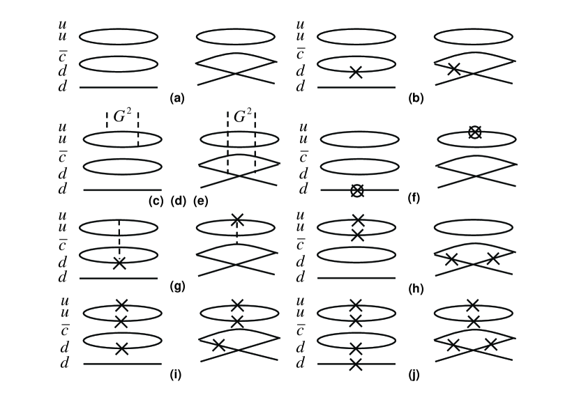
Figure 1: Schematic OPE diagrams for the current $\Theta_{c1}$ in Eq.(1). Each label corresponds to that in Eq.(77). The solid lines denote quark (or anti-charm quark) propagators and the dashed lines are for gluon. The crosses denote the quark condensate, and the crosses with circle represent the mixed quark gluon condensates. (c) represents diagrams proportional to gluon condensate with gluons lines attached to the light quarks only, (d) represents those where the gluons are attached to the heavy quarks only, while (e) represents those where one gluon is attached to the heavy quark and the other to a light quark in all possible ways. (f) and (g) represent all diagrams that contain the quark-gluon condensate.

Our OPE is given by

$$\Pi^{\rm ope,c1}(q) = \Pi^{(a)}+\Pi^{(b)}+\Pi^{(c)}+\Pi^{(d)}+\Pi^{(e)}$$ (47)

$$+\Pi^{(f)}+\Pi^{(g)}+\Pi^{(h)}+\Pi^{(i)}+\Pi^{(j)},$$

where the superscript indicates each diagram in Fig. 1. The imaginary part of each diagram is calculated as

$${1\over\pi}{\rm Im}\Pi^{(a)}(q^{2}) = \frac{11}{5!\,6!\,2^{13}\,\pi^{8}}\int_{0}^{\Lambda}du\,\frac{1}{(1-u)^{5}}\left\{\ooalign{\hfil/\hfil\crcr$q$}\left[-36u(1-u)[-L(u)]^{5}\right.\right.$$

$$+\left.\left.120q^{2}u^{2}(1-u)^{2}[-L(u)]^{4}\right]+m_{c}72[-L(u)]^{5}\right\}\ ,$$

$${1\over\pi}{\rm Im}\Pi^{(b)}(q^{2}) = {5\langle\bar{q}q\rangle\over 4!4!2^{9}\pi^{8}}\int_{0}^{\Lambda}du\frac{1}{(1-u)^{3}}\left\{\ooalign{\hfil/\hfil\crcr$q$}16m_{c}u[-L(u)]^{3}\right.$$

$$+\left.8q^{2}u(1-u)[-L(u)]^{3}-[-L(u)]^{4}\right\}\ ,$$

$${1\over\pi}{\rm Im}\Pi^{(c)}(q^{2}) = -\frac{11\langle\frac{\alpha_{s}}{\pi}G^{2}\rangle}{3\cdot 4!2^{14}\pi^{6}}\int_{0}^{\Lambda}du\frac{1}{(1-u)^{3}}\Bigg{\{}\ooalign{\hfil/\hfil\crcr$q$}\Big{[}-3u(1-u)[-L(u)]^{3}$$

$$+6q^{2}u^{2}(1-u)^{2}[-L(u)]^{2}-\frac{8}{11}(1-u)[-L(u)]^{3}\Big{]}$$

$$+\frac{12}{11}m_{c}[-L(u)]^{3}\Bigg{\}}\ ,$$

$${1\over\pi}{\rm Im}\Pi^{(d)}(q^{2}) = \frac{11\langle\frac{\alpha_{s}}{\pi}G^{2}\rangle}{3!6!2^{12}\pi^{6}}\int_{0}^{\Lambda}du\frac{u^{3}}{(1-u)^{5}}\Bigg{\{}\ooalign{\hfil/\hfil\crcr$q$}m_{c}^{2}\Big{[}-3u(1-u)[-L(u)]^{2}$$

$$+4q^{2}u^{2}(1-u)^{2}[-L(u)]\Big{]}+m_{c}\Big{[}\frac{4}{11}[-L(u)]^{3}$$

$$+\frac{6}{11}q^{2}(1-u)^{2}[-L(u)]^{2}\Big{]}\Bigg{\}}\ ,$$

$${1\over\pi}{\rm Im}\Pi^{(e)}(q^{2}) = \frac{\langle\frac{\alpha_{s}}{\pi}G^{2}\rangle}{4!5!3\cdot 2^{10}\pi^{6}}\int_{0}^{\Lambda}du\frac{u}{(1-u)^{4}}\Bigg{\{}\ooalign{\hfil/\hfil\crcr$q$}\Big{[}\Big{(}96u(1-u)+5(1-u)\Big{)}[-L(u)]^{3}$$

$$-192q^{2}u^{2}(1-u)^{2}[-L(u)]^{2}\Big{]}+90m_{c}[-L(u)]^{3}\Bigg{\}}\ ,$$

$${1\over\pi}{\rm Im}\Pi^{(f)}(q^{2}) = \frac{5\langle\bar{q}g\sigma\cdot Gq\rangle}{3!3!2^{11}\pi^{6}}\int_{0}^{\Lambda}du\frac{1}{(1-u)^{2}}\Big{\{}12\ooalign{\hfil/\hfil\crcr$q$}m_{c}u[-L(u)]^{2}$$

$$-[-L(u)]^{3}+6q^{2}u(1-u)[-L(u)]^{2}\Big{\}}\ ,$$

$${1\over\pi}{\rm Im}\Pi^{(g)}(q^{2}) = \frac{\langle\bar{q}g\sigma\cdot Gq\rangle}{3!4!2^{10}\pi^{6}}\int_{0}^{\Lambda}du\frac{1}{(1-u)^{3}}\Bigg{\{}\ooalign{\hfil/\hfil\crcr$q$}m_{c}\Big{[}12u(1-u)[-L(u)]^{2}$$

$$-60u^{2}[-L(u)]^{2}\Big{]}-12(1-u)[-L(u)]^{3}+72q^{2}u(1-u)^{2}[-L(u)]^{2}$$

$$-\frac{u}{2}[-L(u)]^{3}+3q^{2}u^{2}(1-u)[-L(u)]^{2}\Bigg{\}},$$

$${1\over\pi}{\rm Im}\Pi^{(h)}(q^{2}) = \frac{\langle\bar{q}q\rangle^{2}}{9\cdot 2^{9}\pi^{4}}\int_{0}^{\Lambda}du\frac{1}{(1-u)^{2}}\Bigg{\{}\ooalign{\hfil/\hfil\crcr$q$}\Big{[}12u(1-u)[-L(u)]^{2}$$

$$-16q^{2}u^{2}(1-u)^{2}[-L(u)]+3(1-u)[-L(u)]^{2}\Big{]}+27m_{c}[-L(u)]^{2}\Bigg{\}}\ ,$$

$${1\over\pi}{\rm Im}\Pi^{(i)}(q^{2}) = \frac{5\langle\bar{q}q\rangle^{3}}{9\cdot 2^{4}\pi^{2}}\int_{0}^{\Lambda}du\left\{-\ooalign{\hfil/\hfil\crcr$q$}m_{c}u+[-L(u)]-2q^{2}u(1-u)\right\}\ ,$$ (74)

$${1\over\pi}{\rm Im}\Pi^{(j)}(q^{2}) = \frac{\langle\bar{q}q\rangle^{4}}{216}\left(-\ooalign{\hfil/\hfil\crcr$q$}+22m_{c}\right)\delta(q^{2}-m_{c}^{2}).$$ (77)

Here the upper limit of the integrations is given by $\Lambda=1-m_{c}^{2}/q^{2}$ and $L(u)=q^{2}u(1-u)-m_{c}^{2}u$. Our OPE calculation has been performed up to dimension 12 here. Up to dimension 5, we include all the gluonic contributions represented by the gluon condensate and the quark-gluon mixed condensate. Beyond the dimension 5, we have included only tree-graph contributions which are expected to be important among higher dimensional operators. Other diagrams containing gluon components are expected to be suppressed by the small QCD coupling. Therefore, the higher order tree-graphs, which are the higher order quark condensates, will be able to give us an estimate on how big the typical higher order corrections should be beyond dimension 5. The integrations can be done analytically but we skip the messy analytic expressions. For the charm-quark propagators with two gluons attached, we use the momentum-space expressions given in Ref. Reinders:1984sr . The Wilson coefficients for light-quark condensates come from $\langle\bar{q}q\rangle^{n}$, where $n=2,3,4$. This is in contrast with the OPE for $\Theta_{c2}$, where the Wilson coefficient are non-zero only for $n=4$.

The first important question to ask in the OPE is whether it is sensibly converging as an asymptotic expansion. For that, we choose to plot the Borel transformed OPE appearing in Eq.(14) after subtracting out the continuum contribution,

$$\Pi^{(j)}(M^{2})=\int^{\infty}_{0}dq_{0}~{}e^{-q_{0}^{2}/M^{2}}[\rho_{\rm ope}^{\pm,(j)}(q_{0})-\rho_{\rm cont}^{\pm,(j)}(q_{0})]=0.$$ (78)

Here $j=a,b,c..$ denotes each contribution in the OPE in Eq.(77) after adding according to the rules in Eq.(13).

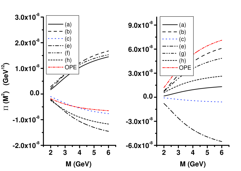
Figure 2: OPE as defined in Eq.(78) for the current $\Theta_{c1}$ and $S_{0}=(3.3~{}{\rm GeV})^{2}$. The left (right) figure is for positive (negative) parity case. The solid line (a) represents the perturbative contribution. The line specified as OPE represents the sum of the power corrections only. (c) represents the gluon condensates. Other labels represent contribution from each term in Eq.(77). Here we plot only a few selected terms in the OPE.

We use the following QCD parameters in our sum rules Shifman:bx ; SDO03 ,

$$m_{s}=0.12~{}{\rm GeV}\ \quad m_{c}=1.26~{}{\rm GeV}\ ,$$ ,

$$\left\langle{\alpha_{s}\over\pi}G^{2}\right\rangle=(0.33~{}{\rm GeV})^{4}\ \quad\langle G^{3}\rangle=0.045~{}{\rm GeV}^{6}\ ,$$ ,

$$\langle\bar{q}q\rangle=-(0.23~{}{\rm GeV})^{3}\ \quad\langle\bar{s}s\rangle=0.8\langle\bar{q}q\rangle\ ,$$ ,

$$\langle\bar{q}g\sigma\cdot Gq\rangle=(0.8~{}{\rm GeV}^{2})\times\langle\bar{q}q\rangle\ \quad\langle\bar{s}g\sigma\cdot Gs\rangle=(0.8~{}{\rm GeV}^{2})\times\langle\bar{s}s\rangle.$$ , (79)

Fig. (2) represents the OPE as defined in Eq.(78) with the imaginary part in Eq.(77). One notes that for the negative parity case, the perturbative contribution is only a small fraction of the OPE, and hence do not converge. For the positive parity case, the power corrections alternate in signs, and the gluon condensate, which represents the light diquark correlation, is only a small correction to the power correction. Hence, such structure, would hardly couple to a pentaquark state, and it is meaningless to perform a detailed QCD sum rule analysis. We present the result with the continuum threshold $S_{0}=(3.3~{}{\rm GeV})^{2}$. This value is chosen in the range $\sqrt{S_{0}}=3.2-3.6$ GeV, which has been used to analyze the anticharmed-pentaquark sum rule in Ref hung04 . However changing $S_{0}$ does not change the relative strength of each contribution, and hence the conclusion of this section. We will therefore, analyze the subsequent OPE with the same threshold.

IV.2 $\Theta_{c2}$

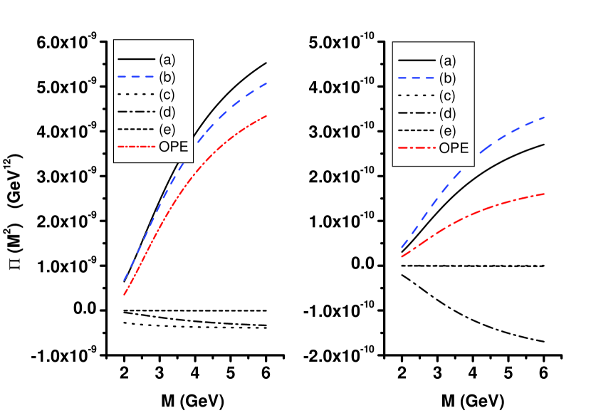
Figure 3: Similar figure as Fig.2 for the current $\Theta_{c2}$. Here each label represents contribution from each term in Eq.(95). The gluon condensates (b) are the dominant power correction in the positive parity channel (left figure).

The OPE for $\Theta_{c2}$ are given in Ref.hung04 . Here, we rewrite the result for completeness,

$${1\over\pi}{\rm Im}\Pi^{(a)}(q^{2}) = -{1\over 5\cdot 5!\ 2^{12}\pi^{8}}\int^{\Lambda}_{0}du\frac{1}{(1-u)^{5}}\left\{\ooalign{\hfil/\hfil\crcr$q$}(1-u)+m_{c}\right\}\ [-L(u)]^{5}\ ,$$ (82)

$${1\over\pi}{\rm Im}\Pi^{(b)}(q^{2}) = -{1\over 3!\ 3!\ 2^{10}\pi^{6}}\left\langle{\alpha_{s}\over\pi}G^{2}\right\rangle\int^{\Lambda}_{0}du\frac{1}{(1-u)^{3}}\left\{\ooalign{\hfil/\hfil\crcr$q$}(1-u)+m_{c}\right\}[-L(u)]^{3}\ ,$$ (85)

$${1\over\pi}{\rm Im}\Pi^{(c)}(q^{2}) = -{1\over 54}\langle\bar{q}q\rangle^{4}(\ooalign{\hfil/\hfil\crcr$q$}+m_{c})~{}\delta(q^{2}-m_{c}^{2})\ ,$$ (88)

$${1\over\pi}{\rm Im}\Pi^{(d)}(q^{2}) = -{1\over 5!\ 3!\ 3\cdot 2^{10}\pi^{6}}\left\langle{\alpha_{s}\over\pi}G^{2}\right\rangle\int^{\Lambda}_{0}du\frac{u^{3}}{(1-u)^{5}}$$ (91)

$$\times \Bigg{\{}3m_{c}^{2}\ooalign{\hfil/\hfil\crcr$q$}(1-u)+m_{c}(1-u)(3-5u)q^{2}+2um_{c}^{3}\Bigg{\}}[-L(u)]^{2}\ ,$$

$${1\over\pi}{\rm Im}\Pi^{(e)}(q^{2}) = -{\left\langle G^{3}\right\rangle\over 5!\ 4!\ 2^{13}\pi^{8}}\int^{\Lambda}_{0}du\frac{u}{(1-u)}~{}\Bigg{\{}\ooalign{\hfil/\hfil\crcr$q$}\left[q^{2}\left({5u\over 2}-1\right)(1-u)-m_{c}^{2}\left({3u\over 2}+7\right)\right]$$ (95)

$$+6m_{c}q^{2}(2u-1)-2m_{c}^{3}{3u+1\over 1-u}\Bigg{\}}[-L(u)].$$

The diagrams corresponding to every term above, denoted by the superscripts $(a)-(e)$, can be found in Ref. hung04 .

Fig. (3) represents the OPE as defined in Eq.(78) with the imaginary part in Eq.(95). As can be seen from the left figure, the OPE without the perturbative contribution is dominated by the gluon condensate coming from the light diquarks. This suggests that the diquark correlation is the dominant interaction among the quarks and heavy antiquark in the positive parity channel. Moreover, the perturbative contribution is larger than sum of the power corrections denoted as “OPE” in the figure. Therefore, the pentaquark could couple strongly to this current and a detailed QCD sum rule analysis is sensible. The situation changes for the negative channel, where the power corrections have alternating signs, and hence becomes less reliable.

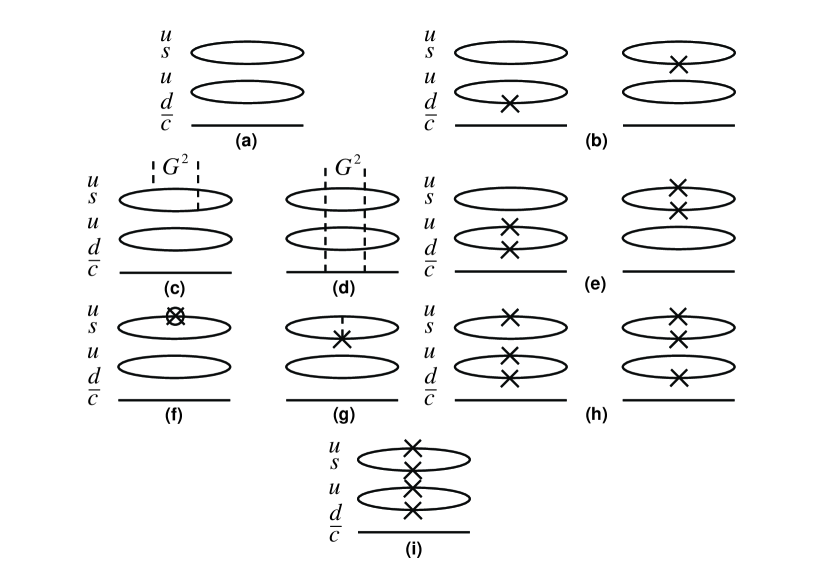
Figure 4: Schematic OPE diagrams for the currents $\Theta_{cs1}$ in Eq.(122) and $\Theta_{cs2}$ in Eq.(149). Each label corresponds to that in Eq.(122) or Eq.(149). All the other notations in this figure are the same as Fig. 1.

IV.3 $\Theta_{cs1}$

The OPE for this current is given as follows

$${1\over\pi}{\rm Im}\Pi^{(a)}(q^{2}) = \frac{1}{5\cdot 5!\,2^{12}\,\pi^{8}}\int_{0}^{\Lambda}du\,\frac{1}{(1-u)^{5}}\left\{\ooalign{\hfil/\hfil\crcr$q$}(u-1)-m_{c}\right\}[-L(u)]^{5}\ ,$$ (98)

$${1\over\pi}{\rm Im}\Pi^{(b)}(q^{2}) = {m_{s}(2\langle\bar{q}q\rangle+\langle\bar{s}s\rangle)\over 3!3!2^{8}\pi^{6}}\int_{0}^{\Lambda}du\frac{1}{(1-u)^{3}}\left\{\ooalign{\hfil/\hfil\crcr$q$}(u-1)-m_{c}\right\}[-L(u)]^{3}\ ,$$ (101)

$${1\over\pi}{\rm Im}\Pi^{(c)}(q^{2}) = \frac{\langle\frac{\alpha_{s}}{\pi}G^{2}\rangle}{3!3!2^{10}\pi^{6}}\int_{0}^{\Lambda}du\frac{1}{(1-u)^{3}}\left\{\ooalign{\hfil/\hfil\crcr$q$}(u-1)-mc\}\right[-L(u)]^{3}\ ,$$ (104)

$${1\over\pi}{\rm Im}\Pi^{(d)}(q^{2}) = -\frac{\langle\frac{\alpha_{s}}{\pi}G^{2}\rangle}{3\cdot 3!5!2^{10}\pi^{6}}\int_{0}^{\Lambda}du\frac{u^{3}}{(1-u)^{5}}\Big{\{}\ooalign{\hfil/\hfil\crcr$q$}3m_{c}^{2}(1-u)$$

$$+m_{c}(1-u)(3-5u)q^{2}+2um_{c}^{3}\Big{\}}[-L(u)]^{2}\,$$

$${1\over\pi}{\rm Im}\Pi^{(e)}(q^{2}) = \frac{(\langle\bar{q}q\rangle^{2}+\langle\bar{q}q\rangle\langle\bar{s}s\rangle)}{3\cdot 2^{7}\pi^{4}}\int_{0}^{\Lambda}du\frac{1}{(1-u)^{2}}\left\{\ooalign{\hfil/\hfil\crcr$q$}(u-1)-m_{c}\}\right[-L(u)]^{2}\ ,$$ (110)

$${1\over\pi}{\rm Im}\Pi^{(f)}(q^{2}) = \frac{m_{s}\langle\bar{q}D^{2}q\rangle}{2^{10}\pi^{6}}\int_{0}^{\Lambda}du\frac{1}{(1-u)^{2}}\left\{\ooalign{\hfil/\hfil\crcr$q$}(u-1)-m_{c}\}\right[-L(u)]^{2},$$ (113)

$${1\over\pi}{\rm Im}\Pi^{(g)}(q^{2}) = \frac{m_{s}\langle\bar{s}g\sigma\cdot Gs\rangle}{3\cdot 2^{11}\pi^{6}}\int_{0}^{\Lambda}du\frac{1}{(1-u)^{2}}\left\{\ooalign{\hfil/\hfil\crcr$q$}(u-1)-m_{c}\}\right[-L(u)]^{2}\ ,$$ (116)

$${1\over\pi}{\rm Im}\Pi^{(h)}(q^{2}) = \frac{m_{s}(2\langle\bar{q}q\rangle^{3}+\langle\bar{q}q\rangle^{2}\langle\bar{s}s\rangle)}{9\cdot 2^{4}\pi^{2}}\int_{0}^{\Lambda}du\left\{\ooalign{\hfil/\hfil\crcr$q$}(u-1)-m_{c}\right\}\ ,$$ (119)

$${1\over\pi}{\rm Im}\Pi^{(i)}(q^{2}) = \frac{\langle\bar{q}q\rangle^{3}\langle\bar{s}s\rangle}{54}\left(\ooalign{\hfil/\hfil\crcr$q$}+m_{c}\right)\delta(q^{2}-m_{c}^{2}).$$ (122)

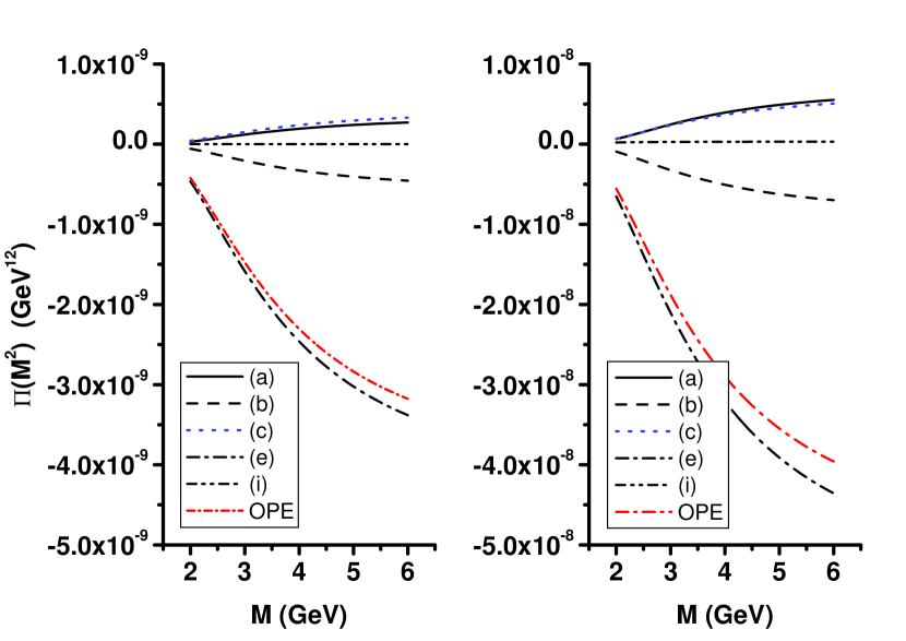
Figure 5: Similar figure as Fig.2 for the current $\Theta_{cs1}$ with $S_{0}=(3.3~{}{\rm GeV})^{2}$. Here each label represents contribution from each term in Eq.(122).

Note here again that the superscripts correspond to the diagrams shown in Fig. 4. The dimension-5 condensate involving $D^{2}$ is related to the quark-gluon condensate via $\langle\bar{q}D^{2}q\rangle=\langle\bar{q}g\sigma\cdot Gq\rangle/2$. Similar relation holds for the corresponding strange-quark condensate. The correction to this relation is proportional to square of the quark mass which should be very small even for the strange quark. Fig. (5) represents the OPE as defined in Eq.(78) with the imaginary part in Eq.(122). We have only included a few terms in the OPE to show how each term contributes differently to the sum rule. As can be seen from the figure, the line denoted as “OPE”, which is sum of the power corrections only, are much larger than the perturbative contribution. Moreover, the gluon condensate from diquarks is only a small fraction of the large higher order correction. This suggests that the OPE are not convergent and it is very unlikely that the diquark correlation will remain an important mechanism in this configuration.

IV.4 $\Theta_{cs2}$

The OPE for this current is given as follows

$${1\over\pi}{\rm Im}\Pi^{(a)}(q^{2}) = \frac{1}{5\cdot 5!\,2^{12}\,\pi^{8}}\int_{0}^{\Lambda}du\,\frac{1}{(1-u)^{5}}\left\{\ooalign{\hfil/\hfil\crcr$q$}(u-1)-m_{c}\right\}[-L(u)]^{5}\ ,$$ (125)

$${1\over\pi}{\rm Im}\Pi^{(b)}(q^{2}) = {m_{s}(-2\langle\bar{q}q\rangle+\langle\bar{s}s\rangle)\over 3!3!2^{8}\pi^{6}}\int_{0}^{\Lambda}du\frac{1}{(1-u)^{3}}\left\{\ooalign{\hfil/\hfil\crcr$q$}(u-1)-m_{c}\right\}[-L(u)]^{3}\ ,$$ (128)

$${1\over\pi}{\rm Im}\Pi^{(c)}(q^{2}) = \frac{\langle\frac{\alpha_{s}}{\pi}G^{2}\rangle}{3!3!2^{10}\pi^{6}}\int_{0}^{\Lambda}du\frac{1}{(1-u)^{3}}\left\{\ooalign{\hfil/\hfil\crcr$q$}(u-1)-mc\}\right[-L(u)]^{3}\ ,$$ (131)

$${1\over\pi}{\rm Im}\Pi^{(d)}(q^{2}) = -\frac{\langle\frac{\alpha_{s}}{\pi}G^{2}\rangle}{3\cdot 3!5!2^{10}\pi^{6}}\int_{0}^{\Lambda}du\frac{u^{3}}{(1-u)^{5}}\left\{\ooalign{\hfil/\hfil\crcr$q$}3m_{c}^{2}(1-u)\right.$$

$$+\left.m_{c}(1-u)(3-5u)q^{2}+2um_{c}^{3}\}\right[-L(u)]^{2}\,$$

$${1\over\pi}{\rm Im}\Pi^{(e)}(q^{2}) = \frac{(\langle\bar{q}q\rangle^{2}-\langle\bar{q}q\rangle\langle\bar{s}s\rangle)}{3\cdot 2^{7}\pi^{4}}\int_{0}^{\Lambda}du\frac{1}{(1-u)^{2}}\left\{\ooalign{\hfil/\hfil\crcr$q$}(u-1)-m_{c}\}\right[-L(u)]^{2}\ ,$$ (137)

$${1\over\pi}{\rm Im}\Pi^{(f)}(q^{2}) = \frac{-m_{s}\langle\bar{q}D^{2}q\rangle}{2^{10}\pi^{6}}\int_{0}^{\Lambda}du\frac{1}{(1-u)^{2}}\left\{\ooalign{\hfil/\hfil\crcr$q$}(u-1)-m_{c}\}\right[-L(u)]^{2},$$ (140)

$${1\over\pi}{\rm Im}\Pi^{(g)}(q^{2}) = \frac{m_{s}\langle\bar{s}g\sigma\cdot Gs\rangle}{3\cdot 2^{11}\pi^{6}}\int_{0}^{\Lambda}du\frac{1}{(1-u)^{2}}\left\{\ooalign{\hfil/\hfil\crcr$q$}(u-1)-m_{c}\}\right[-L(u)]^{2}\ ,$$ (143)

$${1\over\pi}{\rm Im}\Pi^{(h)}(q^{2}) = \frac{m_{s}(-2\langle\bar{q}q\rangle^{3}+\langle\bar{q}q\rangle^{2}\langle\bar{s}s\rangle)}{9\cdot 2^{4}\pi^{2}}\int_{0}^{\Lambda}du\left\{\ooalign{\hfil/\hfil\crcr$q$}(u-1)-m_{c}\right\}\ ,$$ (146)

$${1\over\pi}{\rm Im}\Pi^{(i)}(q^{2}) = \frac{-\langle\bar{q}q\rangle^{3}\langle\bar{s}s\rangle}{54}\left(\ooalign{\hfil/\hfil\crcr$q$}+m_{c}\right)\delta(q^{2}-m_{c}^{2}).$$ (149)

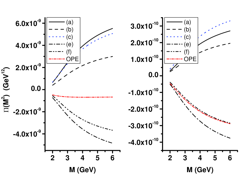
Figure 6: Similar figure as Fig.2 for the current $\Theta_{cs2}$ with $S_{0}=(3.3~{}{\rm GeV})^{2}$. Here each label represents each term in Eq.(149).

Again note that the OPE diagram for each label is shown in Fig. 4. Fig. (6) represents the OPE as defined in Eq.(78) with the imaginary part in Eq.(149). Again, we have only included a few terms in the OPE to show a general trend of each contribution. For the negative parity case, the OPE has large contributions with alternating signs. The situation is better for the positive parity case, but again, the power corrections alternate in signs.

From all the previous analysis on the OPE for the charmed pentaquark with and without strangeness, we find that the one without strangeness with diquark structure are most reliable, and are dominated by gluon condensate coming from diquark correlation. It is interesting to note that this result is consistent with the Skyrme model calculation which predicts a bound state of pentaquarks in the nonstrange sector OPM94 . In the following, we will perform a more detailed analysis with the stable structure well represented by the interpolating current $\Theta_{c2}$.

V QCD sum rules and analysis

V.1 The couplings to the $DN$ continuum, $\lambda_{DN}$

As discussed before, it is important to subtract out the contribution from the $DN$ continuum. For that, one needs to know the coupling strength $\lambda_{DN}$. Here we determine this for the currents without strange quarks, $\lambda_{DN,c2}$. In the case of $\Theta^{+}$ (1540)Lee04 , the soft-kaon theorem was used to convert the external Kaon state, corresponding to the $D$ meson states in Eq.(17) and Eq.(31), to a commutation relation of the operator and the corresponding axial charge. The strength of the resulting five-quark operator with an external nucleon state was then obtained from a separate nucleon sum rule analysis with the same five-quark nucleon current. However, applying the soft $D$ meson limit will obviously not work in the present case.

Instead, we determine the coupling strength directly from the sum rule method. To do that, we eliminate contribution from the low-lying pole by introducing the additional weight $W(q^{2})=q^{2}-m_{\Theta}^{2}$ in Eq.(7). We will take $m_{\Theta}=3$ GeV, and confirmed that changing it by $\pm 200$ MeV will have less than 5 % effect on the $\lambda_{DN}$ value. This way of eliminating a certain pole is sometime used in QCD sum rules jin97 ; ko03 . Then, substituting the corresponding imaginary parts, we find,

$$|\lambda_{DN}|^{2}={\int_{m_{c}^{2}}^{S_{0}}dq^{2}~{}e^{-q^{2}/M^{2}}(q^{2}-m_{\Theta}^{2})\frac{1}{\pi}{\rm Im}\Pi_{i}^{\rm ope}(q^{2})\over\int_{(m_{N}+m_{D})^{2}}^{S_{0}}dq^{2}~{}e^{-q^{2}/M^{2}}(q^{2}-m_{\Theta}^{2})\frac{1}{\pi}{\rm Im}\Pi_{i}^{DN}(q^{2})},\,\,\,(i=1,q)$$ (150)

where the $i=1,q$ in Im$\Pi$ represent the part proportional to $1$ or / $q$ in the respective imaginary part, and Im$\Pi^{DN}$ is the spectral density in Eq.(29) or in Eq.(43) without the $|\lambda_{DN}|^{2}$.

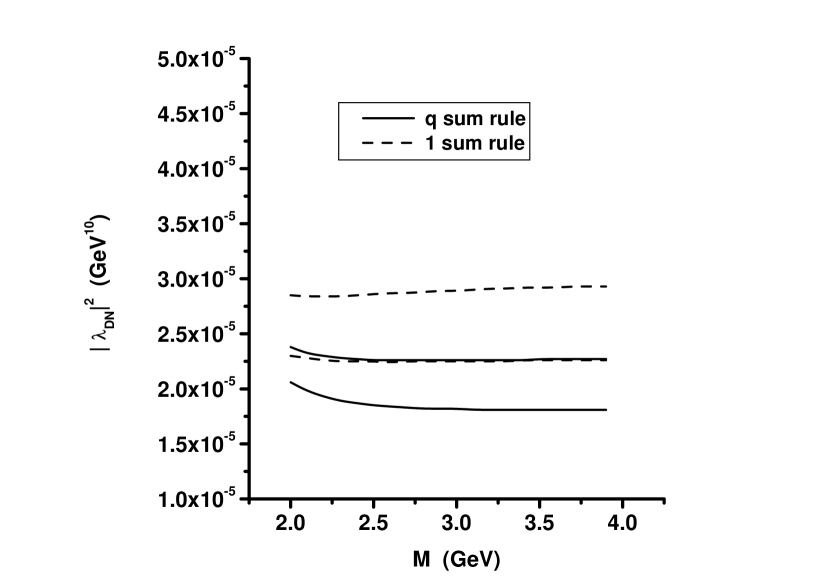
Figure 7: The $|\lambda_{DN,c2}|^{2}$ from the sum rule for $i=q$ (solid) line and $i=1$ (dashed line). The upper (lower) solid or dashed lines in this case are for $S_{0}=(3.8~{}{\rm GeV})^{2}$ [$S_{0}=(3.7~{}{\rm GeV})^{2}$].

Figure (7) shows the plot of Eq.(150). The two dotted (solid) lines represent boundary curves with the least Borel mass dependence for the $\lambda_{DN}$ from the 1 ($q$) sum rules. $\lambda_{DN}$ should not only be independent of the Borel mass but also independent of the sum rule from which it is obtained. However, the results coming from either $i=q$ or $i=1$ sum rule differ slightly. Inspecting the OPE, one finds that the contributions from higher dimensional operators are consecutively suppressed for the $i=q$ sum rule, while that is not so for the $i=1$ sum rule. Therefore, the value from the former sum rule should be more reliable. Nonetheless, to allow for all variations, we will choose the following range for the $|\lambda_{DN}|^{2}$ values,

$$2\times 10^{-5}{\rm GeV}^{10}< |\lambda_{DN,c2}|^{2} <3\times 10^{-5}{\rm GeV}^{10}.$$ (151)

Similar attempts to determine $\lambda_{DN,c1}$ give vastly different values from either $i=q$ or $i=1$ sum rules. This reflects the non-convergence of OPE from which one can not expect a consistent result.

V.2 Parity

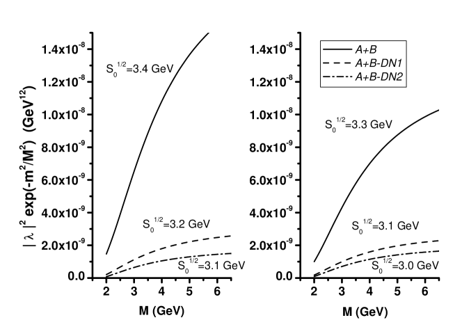
Figure 8: The left figure shows the left-hand side of Eq.(152) using $\Theta_{c2}$ for positive parity case with $|\lambda_{DN,c2}|^{2}=2\times 10^{-5}~{}{\rm GeV}^{10}$ (dashed line) and $|\lambda_{DN,c2}|^{2}=3\times 10^{-5}~{}{\rm GeV}^{10}$ (dot-dashed line). The solid line is when there is no $DN$ continuum, $|\lambda_{DN,c2}|^{2}=0$. The right figure is obtained with different threshold parameters. See Eq. (8) for $A$ and $B$.

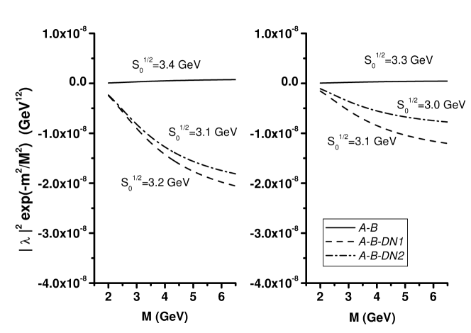
Figure 9: The left figure shows the left-hand side of Eq.(152) using $\Theta_{c2}$ for negative parity case with $|\lambda_{DN,c2}|^{2}=2\times 10^{-5}~{}{\rm GeV}^{10}$ (dashed line) and $|\lambda_{DN,c2}|^{2}=3\times 10^{-5}~{}{\rm GeV}^{10}$ (dot-dashed line). The solid line is when there is no $DN$ continuum. The right figure is obtained with different threshold parameters.

We will now concentrate on the sum rule obtained from $\Theta_{c2}$. Using the dispersion relation in Eq.(14) and the spectral density in Eq.(44), one finds the following sum rule,

$$|\lambda_{\pm,c2}|^{2}e^{-m_{\Theta\pm}^{2}/M^{2}}=\int_{0}^{\sqrt{s_{0}}}dq_{0}~{}e^{-q_{0}^{2}/M^{2}}\bigg{[}\rho_{\rm ope}^{\pm}(q_{0})-\rho_{DN}^{\pm}(q_{0})\bigg{]}\ .$$ (152)

As can be seen from Fig.(8), the left hand side of Eq.(152) is positive for positive parity case. For $|\lambda_{DN,c2}|^{2}=0$ (the solid lines), we have chosen the continuum threshold $S_{0}^{1/2}$ to be 3.4 GeV and 3.3 GeV, which gives the most stable pentaquark mass as we will show in the next subsection. Similar method was used to obtain the continuum thresholds when $|\lambda_{DN,c2}|^{2}\neq 0$. However, Fig.(9) shows that the corresponding sum rule is negative for the negative parity case, suggesting that there can not be any negative parity state. This result also confirms the non-convergence of the OPE for the negative parity case, from which a consistent result can not be obtained. This can also be expected from the constituent quark picture. The two diquarks in $\Theta_{c2}$ current have opposite parities and, when they are combined with the antiquark, the configuration should be dominated by the positive-parity part in the nonrelativistic limit.

V.3 Mass

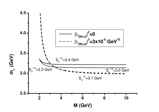
Figure 10: The mass obtained by taking the square root of the inverse ratio between left hand side of Eq.(152) and its derivative with respect to $M^{2}$ using $\Theta_{c2}$.

The sum rule for the $\Theta_{c}$ mass is obtained by taking the derivative of Eq.(152) with respect to $1/M^{2}$. The solid and dashed lines in Fig. (10) represent the mass for two different $\lambda_{DN}$ values. The threshold parameters were obtained to give the most stable mass within the Borel window plotted. One notes that the inclusion of the coupling to the $DN$ continuum states, the mass reduces to smaller values to below 3 GeV. The curve with $\lambda_{DN,c2}=2\times 10^{-5}$ GeV¹⁰ lies between the solid and dashed lines in Fig. (10). This suggests the possibility that the heavy pentaquark might actually be bound; namely, lies below the $DN$ threshold. This is consistent with the constituent quark model picture, where one expects the diquark correlation to be more dominant than that of the quark-antiquark correlation as the participating antiquark becomes heavy. However, if this was the case, its existence can only be measured through its weak decay.

VI summary

We have performed the OPE and QCD sum rule analysis for heavy pentaquark with and without strangeness with two different current each. We find that the OPE is convergent only for the non-strange pentaquark with diquark structure. The OPE for this structure is dominated by gluon condensate coming from diquark, which non-perturbatively represents their strong correlation. We find that the heavy pentaquark without strangeness has positive parity as reported earlierhung04 and that its mass lies below 3 GeV, when the $DN$ irreducible contribution is explicitly including in the phenomenological side of the sum rule. The picture that we described here does not work so well in the light pentaquark $\Theta^{+}$, as the OPE are highly divergentMN04 as can be seen in the picture of the OPE in the original sum rule paper for the light pentaquark stateSDO03 .

References

(1)LEPS Collaboration T. Nakano et al.,
Phys. Rev. Lett. 91 (2003) 012002.
(2)
S. Stepanyan et al. [CLAS Collaboration],
Phys. Rev. Lett. 91 (2003) 252001;
J. Barth et al. [SAPHIR Collaboration],
Phys. Lett. B 572 (2003) 127;
V. V. Barmin et al. [DIANA Collaboration],
Phys. Atom. Nucl. 66 (2003) 1715
[Yad. Fiz. 66 (2003) 1763];
V. Kubarovsky, S. Stepanyan [CLAS Collaboration],
AIP Conf. Proc. 698 (2004) 543;
A. E. Asratyan, A. G. Dolgolenko, M. A. Kubantsev,
Phys. Atom. Nucl. 67 (2004) 682
[Yad. Fiz. 67 (2004) 704]
[arXiv:hep-ex/0309042];
V. Kubarovsky et al. [CLAS Collaboration],
Phys. Rev. Lett. 92 (2004) 032001;
A. Airapetian, et al. [HERMES Collaboration],
Phys. Lett. B 585 (2004) 213;
A. Aleev, et al. [SVD Collaboration],
hep-ex/0401024.
M. Abdel-Bary et al. [COSY-TOF Collaboration],
Phys. Lett. B 595 (2004) 127
[arXiv:hep-ex/0403011];
S. Chekanov et al. [ZEUS Collaboration],
Phys. Lett. B 591 (2004) 7
[arXiv:hep-ex/0403051];
S. Chekanov et al. [ZEUS Collaboration],
Phys. Lett. B 591 (2004) 7
[arXiv:hep-ex/0403051];
Y. Oh, H. Kim and S. H. Lee,
Phys. Rev. D 69, 014009 (2004)
[arXiv:hep-ph/0310019];
Phys. Rev. D 69, 094009 (2004)
[arXiv:hep-ph/0310117];
Phys. Rev. D 69, 074016 (2004)
[arXiv:hep-ph/0311054];
Nucl. Phys. A 745, 129 (2004)
[arXiv:hep-ph/0312229];
S. H. Lee, H. Kim and Y. Oh,
J. Korean Phys. Soc. 46, 774 (2005)
[arXiv:hep-ph/0402135];
Y. Oh and H. Kim,
Phys. Rev. D 70, 094022 (2004)
[arXiv:hep-ph/0405010].
(3)
E. Smith, ”Review on JLAB results”, talk given at Hadron 05,
http://www.cbpf.br/ hadron05/.
(4)
For a review on the present status of pentaquarks, see, K. H. Hicks,
Prog. Part. Nucl. Phys. 55, 647 (2005)
[arXiv:hep-ex/0504027].
(5)
A. Aktas et al. [H1 Collaboration],
Phys. Lett. B 588 (2004) 17
[arXiv:hep-ex/0403017].
(6)
D. O. Litvintsev [CDF Collaboration],
Nucl. Phys. Proc. Suppl. 142, 374 (2005)
[arXiv:hep-ex/0410024].
(7)
U. Karshon [ZEUS Collaboration],
arXiv:hep-ex/0410029.
(8)
J. M. Link et al. [FOCUS Collaboration],
arXiv:hep-ex/0506013.
(9)
D. Diakonov, V. Petrov and M. V. Polyakov,
Z. Phys. A 359, 305 (1997)
[arXiv:hep-ph/9703373].
(10)
T. D. Cohen,
Phys. Lett. B 581, 175 (2004)
[arXiv:hep-ph/0309111].
(11)
C. Gignoux, B. Silvestre-Brac, J. M. Richard,
Phys. Lett. B 193 (1987) 323;
(12)
H. J. Lipkin,
Phys. Lett. B 195 (1987) 484.
(13)
Fl. Stancu,
Phys. Rev. D 58 (1998) 111501;
M. Genovese, J.-M. Richard, Fl. Stancu, S. Pepin,
Phys. Lett. B 425 (1998) 171.
(14)
D. O. Riska, N. N. Scoccola,
Phys. Lett. B 299 (1993) 338.
(15)
Y. Oh, B.-Y. Park, D.-P. Min,
Phys. Lett. B 331 (1994) 362;
Phys. Rev. D 50 (1994) 3350;
Y. Oh, B.-Y. Park,
Phys. Rev. D 51 (1995) 5016;
Y. s. Oh and B. Y. Park,
Z. Phys. A 359, 83 (1997).
(16)
K. Cheung,
Phys. Rev. D 69 (2004) 094029
[arXiv:hep-ph/0308176].
T. E. Browder, I. R. Klebanov, D. R. Marlow,
Phys. Lett. B 587 (2004) 62;
M. A. Nowak, M. Praszalowicz, M. Sadzikowski and J. Wasiluk,
Phys. Rev. D 70 (2004) 031503
[arXiv:hep-ph/0403184];
H. Y. Cheng, C. K. Chua and C. W. Hwang,
Phys. Rev. D 70 (2004) 034007
[arXiv:hep-ph/0403232];
M. E. Wessling,
Phys. Lett. B 603 (2004) 152
[arXiv:hep-ph/0408263];
F. Stancu,
Int. J. Mod. Phys. A 20 (2005) 1797
[arXiv:hep-ph/0504056];
K. Maltman,
Int. J. Mod. Phys. A 20 (2005) 1977
[arXiv:hep-ph/0412327].
(17)
D. Pirjol and C. Schat,
Phys. Rev. D 71, 036004 (2005)
[arXiv:hep-ph/0408293].
(18)
I. W. Stewart, M. E. Wessling and M. B. Wise,
Phys. Lett. B 590, 185 (2004)
[arXiv:hep-ph/0402076].
(19)
R. L. Jaffe and F. Wilczek, Phys. Rev. Lett. 91 (2003) 232003.
(20)
M. Karliner and H. J. Lipkin,
Phys. Lett. B 575 (2003) 249
[arXiv:hep-ph/0402260].
(21)
J. Hofmann and M. F. M. Lutz,
arXiv:hep-ph/0507071.
(22)
T. D. Cohen, P. M. Hohler and R. F. Lebed,
arXiv:hep-ph/0508199.
(23)
R. L. Jaffe,
Phys. Rev. Lett. 38, 195 (1977)
[Erratum-ibid. 38, 617 (1977)].
(24)
E. Hiyama, M. Kamimura, A. Hosaka, H. Toki and M. Yahiro,
arXiv:hep-ph/0507105.
(25)
F. Stancu,
AIP Conf. Proc. 775, 32 (2005)
[arXiv:hep-ph/0504284].
(26)
K. Maltman,
Phys. Lett. B 604, 175 (2004)
[arXiv:hep-ph/0408145].
(27)
S. L. Zhu,
Phys. Rev. Lett. 91 (2003) 232002.
(28)
R. D. Matheus, F. S. Navarra, M. Nielsen, R. Rodrigues da Silva,
S. H. Lee,
Phys. Lett. B 578 (2004) 323.
(29)
J. Sugiyama, T. Doi, M. Oka,
Phys. Lett. B 581 (2004) 167.
(30)
M. Eidemuller,
Phys. Lett. B 597 (2004) 314
[arXiv:hep-ph/0404126].
(31)
H. J. Lee, N. I. Kochelev and V. Vento,
Phys. Lett. B 610 (2005) 50
[arXiv:hep-ph/0412127];
H. J. Lee, N. I. Kochelev and V. Vento,
arXiv:hep-ph/0506250.
(32)
M. Eidemuller, F. S. Navarra, M. Nielsen and R. Rodrigues da Silva,
arXiv:hep-ph/0503193.
(33)
R. D. Matheus, F. S. Navarra, M. Nielsen and R. R. da Silva,
Phys. Lett. B 602 (2004) 185
[arXiv:hep-ph/0406246].
(34)
H. Kim, S. H. Lee and Y. Oh,
Phys. Lett. B 595 (2004) 293
[arXiv:hep-ph/0404170].
(35)
H. Kim and Y. Oh,
Phys. Rev. D 72 (2005) 074012
[arXiv:hep-ph/0508251];
M. E. Bracco, A. Lozea, R. D. Matheus, F. S. Navarra and M. Nielsen,
Phys. Lett. B 624, 217 (2005)
[arXiv:hep-ph/0503137].
(36)
Y. Kondo, O. Morimatsu and T. Nishikawa,
Phys. Lett. B 611 (2005) 93
[arXiv:hep-ph/0404285].
(37)
S. H. Lee, H. Kim and Y. Kwon,
Phys. Lett. B 609 (2005) 252
[arXiv:hep-ph/0411104].
(38)
Y. Kwon, A. Hosaka and S. H. Lee,
arXiv:hep-ph/0505040.
(39)
S. Sasaki,
Phys. Rev. Lett. 93 (2004) 152001
[arXiv:hep-lat/0310014].
(40)
F. Csikor, Z. Fodor, S. D. Katz, T. G. Kovacs,
JHEP 0311 (2003) 070.
(41)
D. Jido, N. Kodama, M. Oka,
Phys. Rev. D 54 (1996) 4532.
(42)
X. M. Jin, J. Tang,
Phys. Rev. D 56 (1997) 515.
(43)
L. J. Reinders, H. Rubinstein, S. Yazaki,
Phys. Rept. 127 (1985) 1.
(44)
M. A. Shifman, A. I. Vainshtein, V. I. Zakharov,
Nucl. Phys. B 147 (1979) 385.
(45)
X. m. Jin,
Phys. Rev. D 55, 1693 (1997)
[arXiv:hep-ph/9608303].
(46)
H. Kim and M. Oka,
Nucl. Phys. A 720, 368 (2003)
[arXiv:hep-ph/0301227].