Abstract

In Universal Extra Dimension models, the lightest Kaluza-Klein (KK) particle is generically the first KK excitation of the photon and can be stable, serving as particle dark matter. We calculate the thermal relic abundance of the KK photon for a general mass spectrum of KK excitations including full coannihilation effects with all (level one) KK excitations. We find that including coannihilation can significantly change the relic abundance when the coannihilating particles are within about 20% of the mass of the KK photon. Matching the relic abundance with cosmological data, we find the mass range of the KK photon is much wider than previously found, up to about 2 TeV if the masses of the strongly interacting level one KK particles are within five percent of the mass of the KK photon. We also find cases where several coannihilation channels compete (constructively and destructively) with one another. The lower bound on the KK photon mass, about 540 GeV when just right-handed KK leptons coannihilate with the KK photon, relaxes upward by several hundred GeV when coannihilation with electroweak KK gauge bosons of the same mass is included.

1 Introduction

One of the most important astrophysical challenges is to understand the nature and identity of dark matter. Perhaps the most interesting candidate is a neutral, stable, weakly interacting particle arising from physics beyond the Standard Model. This is consistent with a wide range of data, such as measurements of the cosmic microwave background (CMB) radiation that imply the abundance of dark matter is roughly a factor of 6 times the abundance of baryons [1], as well as comparisons between large scale structure simulations and galaxy survey observations that suggest the bulk of dark matter is cold [2].

Universal Extra Dimension (UED) models [3] (see also [4]), in which all of the Standard Model fields propagate in extra dimensions, provide an interesting example of Kaluza-Klein (KK) dark matter [5, 6, 7]. This is because bulk interactions do not violate higher dimensional momentum conservation (KK number), and in these models all of the couplings among the Standard Model particles arise from bulk interactions. To generate 4D chiral fermions, the extra compact dimension(s) must be modded out by an orbifold. For five dimensions this is $S^{1}/Z_{2}$, while in six dimensions $T^{2}/Z_{2}$ is suitable and has other interesting properties [3] including motivation for three generations from anomaly cancellation [8] and the prevention of fast proton decay [9]. An orbifold does, however, lead to some of the less appealing aspects of the model. Brane-localized terms can be added to both orbifold fixed points that violate KK number. If these brane localized terms are symmetric under the exchange of the two orbifold fixed points, then a remnant of KK number conservation remains, called KK parity. All odd-level KK modes are charged under this discrete symmetry thereby ensuring that the lightest level-one KK particle (LKP) does not decay. The stability of the LKP suggests it could well be an interesting dark matter candidate.

We calculate the thermal relic abundance of dark matter including coannihilation with all level-one KK particles. This is an important calculation since there are many level-one KK particles that are near enough in mass to the LKP that they are expected to be important to determine the relic abundance. The identity of the LKP depends on the mass spectrum of the first KK level. We assume it is the lightest KK photon. This has been widely advocated for both its properties as dark matter and is favored by the contributions to the masses of the level one KK particles from one-loop radiative corrections [5, 7]. The spectrum of level-one KK particle masses is also not known. However, certain finite and log-enhanced one-loop radiative corrections [10] to the masses have been calculated in [5]. The size of these corrections depend on two unknowns: the size of the log, i.e., the cutoff scale of the theory, and the size of the matching corrections evaluated at the cutoff scale. Generically one would expect the calculable log-enhanced corrections to dominate over the uncalculable matching corrections. However, the log is not particularly large relative to the finite matching corrections. Indeed, should the cutoff scale be close to the scale of the KK particle masses, uncalculable matching corrections would be of order the calculable log-enhanced corrections, and then one would like to know the relic abundance for a general spectrum. This is the calculation we carry out in this paper.

We present our results with three scenarios of level-one KK particle mass spectra. First, we consider coannihilation with all level-one KK particles that carry electroweak, but not color charges. Next, we consider coannihilation including colored particles. In both of these cases, we take all of the level one KK particles (other than the LKP) to have the same mass $m_{\gamma^{(1)}}(1+\delta)$. Finally, we consider coannihilation with all particles with a mass spectrum derived from the loop corrections from [5]. We believe these three scenarios provide a good cross section of the effects of coannihilation. We also provide formulae for the (co)annihilation cross sections so that any other more complicated spectra could easily be calculated based on our results.

The format of this paper is as follows. In Sec. 2 we discuss KK dark matter including past results and motivate the need for the calculations we carry out. In Sec. 3, we briefly describe the method used to calculate the relic abundance of the KK photon, and the effect of including coannihilating particles in this calculation. In Sec. 4, we consider the effect of coannihilation on the relic abundance, and use this to obtain limits on the mass of the corresponding dark matter candidate, the KK photon. We find mass ranges in three scenarios: (1) when electroweak KK excitations coannihilate, (2) when all KK excitations coannihilate, taking all KK particles (except for the LKP) to have the same mass, and (3) when all KK excitations coanihilate assuming the mass spectrum is determined by the one-loop radiative corrections in [5] with zero matching corrections. Appendices A and B reviews the Lagrangian and Feynman rules in UED. The diagrams and cross sections pertinent to these results are summarized in Appendices C and D.

2 KK dark matter

The relic density of the KK photon was first calculated by Servant and Tait [6]. Using their results, one finds that its thermal relic abundance of the KK photon matches the WMAP observations for cold dark matter when the KK photon mass is between about 550 to 850 GeV. The range of mass that they found depended on the relative importance of coannihilation with the level-one KK excitations of the right-handed leptons. This was the only coannihilation channel that was considered in [6]. Several groups have also examined the prospects for detecting KK dark matter directly and indirectly [7].

Coannihilation is likely to occur through other level one KK excitations. Examining a typical spectrum of KK excitations from the one-loop radiative corrections discussed in [5], one finds that the KK excitations of the particles transforming under the electroweak (but not color) groups tend to be within about 10% of the mass of the KK photon. This is near enough in mass that coannihilation with these KK excitations is expected to affect the the thermal relic abundance. We emphasize that these radiative corrections, proportional to the log of the ratio of the cutoff scale $\Lambda$ to the compactification scale $R^{-1}$, are merely indicative of shifts in the level one KK particle masses, since the finite matching corrections are unknown. Indeed, if the cutoff scale were not too large, even the KK excitations that transform under SU(3)_c could also play an important role in the calculation of the thermal relic abundance.

What is the cutoff scale of UED models? Generically, the cutoff scale is where the extra dimensional theory gets strong. In the four dimensional effective theory this can be estimated by including KK excitations into loops, and one obtains typically $\Lambda R\sim 10$–$100$. But there have also been recent explicit scattering amplitude calculations that suggest the cutoff scale may be much lower than previously assumed [11]. In any case, it is clear that including the effects of coannihilation for the entire spectrum will allow us to calculate the broadest range of KK photon masses that lead to a thermal relic abundance consistent with the cosmological measurements. We will illustrate the relative importance of different channels by showing the results for specific choices of the level one KK spectrum.

The lower bound on the mass of the KK photon arises by calculating the effects of KK particles in loop corrections to precision electroweak data. This was first done by [3] who found a lower bound of about $300$ GeV. As we will see, this bound is not saturated no matter what spectrum of level one KK excitations one takes, and so we do not need to consider it further.

In general, the accuracy we desire requires only tree-level calculations. However a very recent paper did find an important effect on the relic abundance of the KK photon [12]. The loop suppressed operators on the orbifold fixed points lead to couplings between pairs of level-one excitations and SM particles through resonances of level two (and higher) KK excitations. The resonance behavior can roughly compensate for the loop suppression, resulting in a large contribution to the total cross section. Ref. [12] investigated the effect of the annihilation $\gamma^{(1)}\gamma^{(1)}\rightarrow t\bar{t}$ through an $s$ channel $h^{(2)}$, and found that including this process leads to a significant decrease in the relic abundance of $\gamma^{(1)}$. Including these loop-suppressed effects would make our calculations prohibitively complicated, so in this paper we neglect them. Instead, our motivation is orthogonal, namely to understand the implications of including coannihilation of all level one KK excitations on the relic abundance. Ultimately, to obtain the most accurate estimate of the relic abundance of the KK photon would require taking into account both the resonance effect as well as the coannihilation effects that we report in this paper.

3 The Relic Density of the KK photon

3.1 Annihilation and freeze-out

We now briefly review the standard method for calculating the cosmological relic density of a stable particle [13, 14]. The number density of a particle in the expanding universe is described by the Boltzmann equation

$$\frac{dn_{\psi}}{dt}+3Hn_{\psi}=-\left<\sigma_{A}v\right>\left[(n_{\psi})^{2}-(n_{\psi}^{eq})^{2}\right]$$ (1)

where $\left<\sigma_{A}v\right>$ is the thermal average of the total cross section for annihilation of the particle $\psi$ (assumed here to be equal to the total cross section for producing $\psi$) times the relative velocity of two particles, and $H$ is the Hubble expansion rate of the universe.

We solve the Boltzmann equation to obtain the number density of a massive particle at late times. At early times ($T\gg m_{\psi}$, $n_{\psi}^{eq}\approx T^{3}$), $n_{\psi}^{eq}$ is large, and any deviation of $n$ from $n^{eq}$ rapidly goes to $0$. At late times ($T\ll m_{\psi}$, $n_{\psi}^{eq}\approx g(m_{\psi}T/2\pi)^{3/2}e^{-m_{\psi}/T}$), $n^{eq}$ is tiny since the particles are now too massive to be thermally produced. As $n_{\psi}$ decreases due to the expansion of the universe, the particles eventually become too dilute to annihilate and freeze out at a constant density per comoving volume. This freeze-out occurs roughly when the Hubble expansion rate overtakes the rate at which the particles annihilate, $\Gamma=\left<\sigma_{A}v\right>n_{\psi}\approx H$.

As we will verify later, KK dark matter freezes out at $T_{f}\ll m_{KK}$, so that at freeze out $n^{eq}=g\left(\frac{m^{2}}{2\pi x}\right)^{3/2}e^{-x}$, where $x=\frac{m}{T}$, and $g$ is the number of degrees of freedom of the annihilating particle. In this case, (1) cannot be solved analytically. Instead, the Boltzmann equation must be solved either numerically, or by means of a standard approximation which gives solutions consistent with numerical results to within $10\%$. Here we shall use the latter approach.

To solve the Boltzmann equation approximately, we begin by making a simplifying change of coordinates. If we assume the universe expands adiabatically, then $sa^{3}=$ constant, where $s$ is the comoving entropy density given by $s=\frac{2\pi^{2}}{45}g_{*}T^{3}$ and $g_{*}$ is the effective number of relativistic degrees of freedom. In terms of the variables $Y=n_{\psi}/s$, $Y^{eq}=n^{eq}/s$, and $x=m/T$, (1) can be rewritten as

$$\frac{dY}{dx}=-\frac{\left<\sigma_{A}v\right>}{Hx}s[Y^{2}-(Y^{eq})^{2}]$$ (2)

where we assume that freeze-out occurs in a radiation dominated epoch, so that $\frac{dx}{dt}=Hx$. Writing $\Delta=Y-Y^{eq}$, this becomes

$$\Delta^{\prime}+{Y^{eq}}^{\prime}= -C\frac{\left<\sigma_{A}v\right>}{x^{2}}\Delta(2Y^{eq}+\Delta)$$

$$= -f(x)\Delta(2Y^{eq}+\Delta)$$ (3)

where $C=\sqrt{\frac{g_{*}\pi}{45}}mM_{\rm Pl}$, and $f(x)=C\left<\sigma_{A}v\right>x^{-2}$.

At early times, the particles track their equilibrium values, so that $\Delta\ll Y^{eq}$ and $\Delta^{\prime}\ll{Y^{eq}}^{\prime}$. In this case

$$\Delta=-\frac{{Y^{eq}}^{\prime}}{f(x)(2Y^{eq}+\Delta)}$$ (4)

To determine the freeze-out temperature, we use this expression for $\Delta$ to solve $\Delta=cY^{eq}$ with $Y^{eq}=\frac{45g}{\sqrt{32\pi^{7}}g_{*}}x^{3/2}e^{-x}$, where $c$ is a numerical factor whose optimal value is determined by comparison with numerical solutions of the Boltzmann equation ($c=\sqrt{2}-1$). The freeze-out temperature can be deduced by solving the following equation numerically:

$$x_{f}=\ln\left(c(c+2)\sqrt{\frac{45}{8}}\frac{gmM_{\rm Pl}\langle\sigma_{A}v\rangle}{2\pi^{3}\sqrt{g_{*}x_{f}}}\right)$$ (5)

At late times, $Y^{eq}$ and ${Y^{eq}}^{\prime}$ are both small, and the equation reduces to

$$\frac{\Delta^{\prime}}{\Delta^{2}}=-f(x)$$ (6)

This equation is separable, and can thus be solved (with boundary conditions again chosen to give the best fit to numerical simulations):

$$Y_{\infty}\approx\Delta_{\infty} = \frac{1}{\int_{x_{f}}^{\infty}f(x)dx}$$

$$\rho_{\psi}=m_{\psi}n_{\psi}|_{t=\infty} = m_{\psi}s_{0}Y_{\infty}$$

$$\Omega_{\psi}=\frac{\rho_{\psi}}{\rho_{c}} = \frac{s_{0}\sqrt{45}}{\sqrt{\pi g_{*}}M_{\rm Pl}\rho_{c}\int_{x_{f}}^{\infty}\left<\sigma_{A}v\right>x^{-2}dx}$$ (7)

$$\approx \frac{1.04\times 10^{9}}{\int_{x_{f}}^{\infty}\left<\sigma_{A}v\right>x^{-2}dx}$$

Note that because of the factor of $s_{0}$ appearing in the numerator, this solution assumes that the universe expands adiabatically between freeze-out and today. This is, of course, not quite true, as some standard model particles will subsequently fall out of equilibrium, slightly increasing the entropy per comoving volume. In practice, however, this contribution from known standard model sources is very small, and hence may safely be neglected.

3.2 Coannihilation

Different species of interacting particles that have masses nearly degenerate with the KK photon will fall out of equilibrium at the same time and with roughly similar density. Interactions of the form $\psi_{1}X\rightleftharpoons\psi_{2}X^{\prime}$ (where $\psi_{1}$ and $\psi_{2}$ are the KK particles, and $X,X^{\prime}$ are SM particles), converting the relic into other particles of similar mass, occur rapidly. In fact, such processes are much more efficient than the relevant annihilation processes, so that the abundances of the all particles are effectively correlated during freeze-out. The slightly heavier particle species will eventually all decay to the lightest stable particle (in our case, the KK photon) and thus contribute to the relic density. This situation is called coannihilation.

As shown in [14], to compute the relic density and freeze-out temperature with coannihilation, it suffices to substitute an effective cross section $\sigma_{\rm eff}$ for $\sigma$ in Eqs. (3.1),(5) above, where

$$\sigma_{\rm eff}=\sum_{i,j}\sigma_{ij}\frac{g_{i}g_{j}}{g_{\rm eff}^{2}}(1+\Delta_{i})^{3/2}(1+\Delta_{j})^{3/2}e^{-x(\Delta_{i}+\Delta_{j})}$$

$$g_{\rm eff}=\sum_{i}g_{i}(1+\Delta_{i})^{3/2}e^{-\Delta_{i}x}$$ (8)

The relic abundance depends on a weighted average of the annihilation and coannihilation cross sections of all relevant particles. Thus if the coannihilating particles interact more strongly compared with the annihilating particles (while also being close enough in mass) they can increase the effective cross section and thereby decrease the relic density. Conversely, if they are more weakly interacting, then the coannihilation effects decrease the effective cross section, yielding a larger final value for $\Omega_{\psi}$.

A simple intuitive picture of the effects of including coannihilation comes from noting that

$$\rho\sim\left(\int_{x_{f}}^{\infty}\left<\sigma_{A}v\right>x^{-2}\right)^{-1}.$$ (9)

The integral over $x$ will of course result in a different weight for $s$ and $p$ wave annihilation, nevertheless it is easiest to simply ignore this difference and approximate $\rho_{\psi}\sim(\left<\sigma v\right>)^{-1}$. A larger effective cross section results in more annihilation during freeze-out, and thus a smaller relic density.

Furthermore, it is easy to see that the effective cross section $\sigma_{\rm eff}$ is a weighted average of the relevant annihilation and coannihilation cross sections by considering the case where all but the lightest (first) coannihilating particles have the same mass $m_{j}=m_{0}(1+\delta)$, $j\neq 1$, and all particles have the same number of degrees of freedom. Then

$$A = \frac{\sum\limits_{ij}(1+\delta)^{3(a_{i}+a_{j})/2}e^{-(a_{i}+a_{j})\delta x}\frac{\sigma_{ij}}{\sigma_{11}}}{\sum\limits_{i}(1+\delta)^{3a_{i}/2}e^{-a_{i}x\delta}}$$

$$\delta\rightarrow 0 \Rightarrow \frac{1}{N^{2}}\sum_{ij}\frac{\sigma_{ij}}{\sigma_{11}}$$ (10)

where $i,j$ run over all included particles, $a_{i,j}=0(1)$ for the LKP (all other KK particles), and $\sigma_{ij}$ is the total (co)annihilation cross section for the process $\psi_{i}\psi_{j}\rightarrow$ Standard Model particles.

This makes it clear that in the limit of a small mass difference and equal numbers of degrees of freedom, $\sigma_{\rm eff}$ is precisely the average of all relevant cross sections while the relic abundance depends only on whether this average is larger or smaller than $\sigma_{11}$. If all $\sigma_{ij}$ are equal, then including coannihilation does not alter the relic density; if the weighted cross sections of the coannihilating particles are on average larger (smaller) than that of the original particle, then the relic density will be smaller (larger) when coannihilation is included. This holds irrespective of the value of $\delta$. However, since $\delta$ enters exponentially into the weights of the coannihilation cross sections, the effects of coannihilation are rapidly suppressed as the relative mass difference $\delta$ increases. Typically for weakly interacting particle dark matter, $x_{f}\approx 20$ to $30$, and for $\delta>0.1$ the effects of coannihilation are generally negligible. However, for very large coannihilating cross sections, fractional mass differences up to $\delta=0.2$ can affect the relic density [14].

4 Results

Now we are ready to consider the effect of coannihilation on the relic abundance of the the KK photon. Each coannihilation scenario considered requires several total annihilation cross sections; the relevant Feynman diagrams, together with tables of the formulae of the relevant cross sections, are presented in Appendices C and D.

Certain approximations were made in obtaining our results. Cross sections were computed ignoring all terms of order $\frac{m_{SM}}{m_{KK}}$ where $m_{SM}$ is any standard model mass. Consequently, we ignored all Yukawa couplings which are proportional to the corresponding fermion mass. This approximation is well justified (in that including such terms should alter the relic abundance by less than $10\%$) for all particles except possibly the top quark, whose mass $m_{t}\approx 175$ GeV is close to one half of the precision electroweak lower bound on $R^{-1}$. In particular, as shown in [12], the top Yukawa coupling can alter the cross section significantly, as it leads to nearly resonant $s$-channel diagrams. Aside from this effect, our results are not expected to be sensitive to the top mass since, as we will see, the masses of the KK photon necessary to explain the observed relic dark matter abundance are well above the mass of the top quark. It addition, we neglected the mixing between $B^{(1)}$ and $W^{3(1)}$, which are expected to be rather small already for the first KK level (see Appendix A.3). Hence, we take $\gamma^{(1)}\equiv B^{(1)}$, $Z^{(1)}\equiv W_{3}^{(1)}$ throughout.

When examining the relic density as a function of mass, a further simplification is obtained by ignoring the mass-dependence of $x_{f}$. The value of $x_{f}$ depends very weakly on the mass. Indeed, from (5) we expect this dependence to be approximately logarithmic. Typically, over the mass range of $m_{KK}=0.2$ to $2$ TeV, $x_{f}$ varies by about $2$ GeV/degree, or less than 10%. This variation has a small effect on the relic density. This also shows that the KK dark matter is cold: for all cases considered here, we find $23<x_{f}<28$, so that the particles are well approximated as non-relativistic.

We use couplings and astrophysical parameters that can be obtained from [15]. In particular, we take the electroweak and strong couplings evaluated at $M_{Z}$ (ignoring the renormalization group running of the couplings). In practice, the freeze-out temperature is between about $25$ and $100$ GeV, depending on which particles coannihilate. The dark matter relic density is taken to be the $1\sigma$ value from WMAP, $\Omega_{DM}=0.113\pm 0.01$ [1].

4.1 Coannihilation with simplified level-one KK spectrum

To investigate the effects of KK particles coannihilating with the KK photon, we chose two different mass spectra for the coannihilating particles. First, particles in the first KK level are divided into two groups: those with masses approximately $m_{\gamma^{(1)}}(1+\delta)$, with $\delta$ small, and those that are too heavy to play a role in coannihilation. While this choice of mass spectrum gives a good understanding of the range of possible outcomes of including coannihilating particles, it is also somewhat arbitrary. Thus, we also investigate a mass spectrum based on that derived in [5] in the next subsection.

The first check on our results was to consider coannihilation of the KK photon with just right-handed leptons, where our calculations and numerical results agree with [6]. This provides a non-trivial check on our procedure for calculating the relic density in the Universal Extra Dimensions model.

Figure 1 shows the effect of including coannihilation of the KK photon with leptons (blue), and all electroweak particles including leptons, scalars, and electroweak gauge bosons (red). Here we assume in each case that particles included in the coannihilation have the same mass $m_{\gamma}(1+\delta)$. The graph shows that coannihilation with leptons, and to a lesser extent with $W$ and $Z$ bosons, tends to increase the relic density for a given mass of the KK photon.

Figure 2 shows the effect of including coannihilation of the KK photon with all level one KK electroweak particles and level one KK quarks (blue), and all particles at KK level one including the KK gluon (red). Again, we assume in each case that all particles included in the coannihilation have the same mass $m_{\gamma}(1+\delta)$. Clearly, including coannihilation with strongly interacting KK particles decreases the relic abundance for a fixed KK photon mass. The extent of this decrease is one of the most important results of this paper. In particular, if the level one KK particles are highly degenerate to within a few to perhaps 10%, the KK photon mass consistent with the thermal relic abundance that matches the WMAP data could be several TeV.

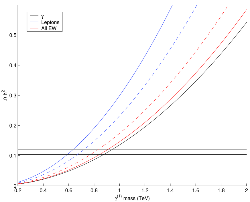
Figure 1: Relic abundance of KK dark matter as a function of mass after including no coannihilation (black; right-most solid line), coannihilation of $B^{(1)}$ with all leptons (blue; left-most pair of solid and dashed lines), and all electroweak particles (red; middle pair of solid and dashed lines), assuming in each case that all coannihilating particles have the same mass $m_{\gamma^{(1)}}(1+\delta)$. The solid (dashed) lines show the values for $\delta=0.01$ $(0.05)$ for the cases with coannihilation. Notice that for the case including KK electroweak gauge bosons, the abundance as a function of mass is smaller for the smaller mass splitting $\delta=0.01$, unlike the case with just KK leptons, since the effects of coannihilation of these two sets of KK particles somewhat compensate for each other in the relic abundance calculation.

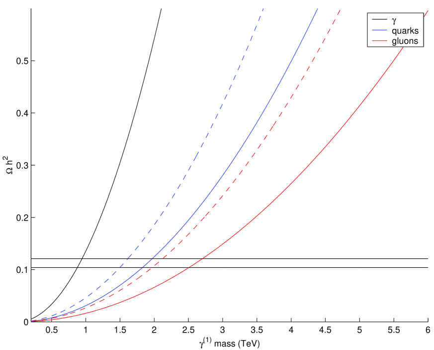
Figure 2: Relic abundance of KK dark matter as a function of mass after including coannihilation of $B^{(1)}$ with all non-strongly interacting particles and quarks (blue), and all level one particles (red) assuming in each case that all coannihilating particles have the same mass $m_{\gamma^{(1)}}(1+\delta)$. The solid and dashed lines show the values for $\delta=0.01$, and $\delta=0.05$.

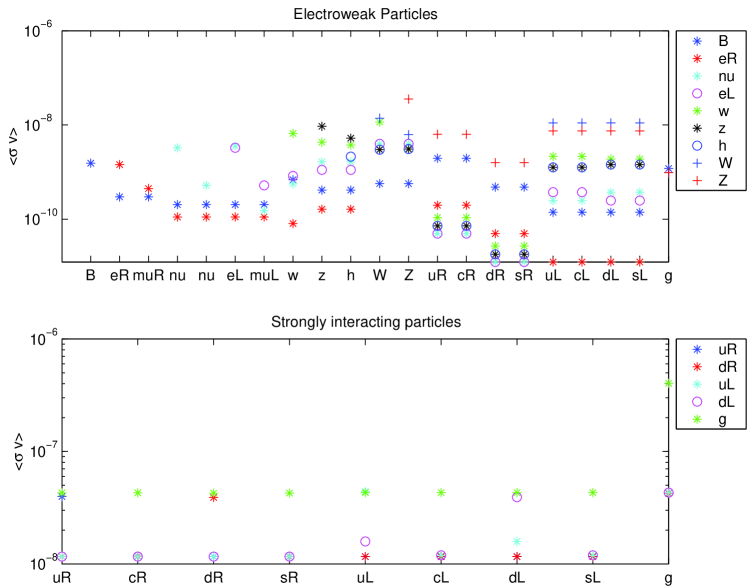
Figure 3: Magnitudes of all cross sections, using $m_{KK}=1$ TeV, $x_{f}=25$, and all couplings taken at the scale $M_{Z}$. Here each color represents a particular particle species (see legend), and the x-axis indicates with which particle the (co)annihilation is occurring. For example, a blue dot above the text $e_{L}$ is the coannihilation cross section of $B^{(1)}\equiv\gamma^{(1)}$ with $e_{L}$. Only 2 families of fermions are shown, as this is sufficient to show the difference between annihilation between members of the same family, and coannihilation between members of different families. The annihilation cross sections for fermions, $W$ and its scalar counterpart $w$ have been weighted by a factor of $1/2$ to account for the two helicities. In general the coannihilation cross sections are smaller than the annihilation ones, (and more numerous) so that usually adding more coannihilating particles decreases the effective cross section. However, as the SU(2) coupling is stronger than the U(1) coupling, and as it also opens more channels, when scalars and gauge bosons, whose annihilation cross sections are quite large, are added, the average cross section increases.

These results can be more readily understood by examining the relative magnitudes of the cross sections in question, shown in in Fig. 3. Notice first that the coannihilation cross section of any non-colored particle with $B^{(1)}$ is smaller than the annihilation cross section of $B^{(1)}$ with itself. Thus coannihilation with particles whose self-annihilation cross sections are close to those of $B^{(1)}$ tends to decrease the effective cross section, and hence increase the relic abundance for a given $B^{(1)}$ mass. This is the case for leptons and scalars. The level one KK electroweak gauge bosons $W^{(1)}$ and $Z^{(1)}$ and all strongly interacting particles have sufficiently large self-annihilation cross sections that they cause an increase in the effective cross section, and decrease the relic abundance. For $W^{(1)}$ and $Z^{(1)}$ this effect is relatively small, and their inclusion does not completely counter-balance the reduction in $\sigma_{eff}$ resulting from including leptons and scalars. In the case of the strongly interacting particles, the relevant cross sections are approximately an order of magnitude larger than those of the non-strongly interacting particles, and the resulting reduction in the relic density is quite dramatic at small $\delta$.

4.2 Coannihilation with the Cheng, Matchev, Schmaltz spectrum

In this section we consider the spectrum that results if one takes the one-loop radiative corrections to the KK masses from [5]. There are several assumptions built into this spectrum. One is that the matching contributions to the brane-localized kinetic terms are assumed to be zero when evaluated at the cutoff scale. Furthermore, the radiatively generated terms are log enhanced by a log of the ratio of the cutoff scale $\Lambda$ to the mass of the KK excitation. This ratio is also not known, and may be much smaller than previously estimated [11]. We therefore consider a wide range of $\Lambda R$ to illustrate the effects of coannihilation.

First, let us summarize the results of [5] that are used for the masses of the KK excitations in this Section:

$$\delta(m^{2}_{B^{(n)}}) = \frac{g^{\prime 2}}{16\pi^{2}R^{2}}\left(\frac{-39}{2}\frac{\zeta(3)}{\pi^{2}}-\frac{n^{2}}{3}\ln\,\Lambda R\right)$$

$$\delta(m^{2}_{W^{(n)}}) = \frac{g^{2}}{16\pi^{2}R^{2}}\left(\frac{-5}{2}\frac{\zeta(3)}{\pi^{2}}+15n^{2}\ln\,\Lambda R\right)$$

$$\delta(m^{2}_{g^{(n)}}) = \frac{g_{s}^{2}}{16\pi^{2}R^{2}}\left(\frac{-3}{2}\frac{\zeta(3)}{\pi^{2}}+23n^{2}\ln\,\Lambda R\right)$$

$$\delta(m_{Q^{(n)}}) = \frac{n}{16\pi^{2}R}\left(6g_{s}^{2}+\frac{27}{8}g^{2}+\frac{1}{8}g^{\prime 2}\right)\ln\,\Lambda R$$

$$\delta(m_{u^{(n)}}) = \frac{n}{16\pi^{2}R}\left(6g_{s}^{2}+2g^{\prime 2}\right)\ln\,\Lambda R$$

$$\delta(m_{d^{(n)}}) = \frac{n}{16\pi^{2}R}\left(6g_{s}^{2}+\frac{1}{2}g^{\prime 2}\right)\ln\,\Lambda R$$

$$\delta(m_{L^{(n)}}) = \frac{n}{16\pi^{2}R}\left(\frac{27}{8}g^{2}+\frac{9}{8}g^{\prime 2}\right)\ln\,\Lambda R$$

$$\delta(m_{e^{(n)}}) = \frac{n}{16\pi^{2}R}\frac{9}{2}g^{\prime 2}\ln\,\Lambda R$$ (11)

All of the non-colored KK excitation masses are within about 10% of $m_{\gamma^{(1)}}$ up to moderately high values of the cutoff scale ($\Lambda R\approx 30$), and hence are almost certainly relevant for coannihilation. Conversely, for $\Lambda R>5$, the masses of the strongly interacting particles are more than $10\%$ greater than $m_{\gamma^{(1)}}$, and thus are less likely to be important for coannihilation. However, as emphasized by [14], particles with sufficiently large cross sections may be relevant to coannihilation even for mass differences of up to of order $20\%$.

We further simplify the mass spectrum given by (4.2), while ignoring the SM top quark mass, by dividing the KK particles into five mass classes: the KK photon; the KK leptons and scalars; the KK $W$ and $Z$ gauge bosons; the KK quarks; and the KK gluon. (In cases with more than one particle of slightly differing mass, we take the average mass of all of the particles in that class.)

Figure 4 shows the $\gamma^{(1)}$ mass that results in a thermal relic abundance consistent with cosmological data, as a function of $\Lambda R$, given a five class mass spectrum. The upper plot also shows the mass gap $\delta$ for each of the classes. Because $g_{s}$ is considerably larger than $g,g^{\prime}$, the masses of the strongly interacting particles increase rather quickly as the cutoff increases. For $\Lambda R\geq 2$, nearly all strongly interacting particles have $\delta>0.05$. Masses of the leptons and scalars, however, vary rather slowly with $\Lambda R$, and remain within $10\%$ of the $\gamma^{(1)}$ mass out to values $\Lambda R\sim 10^{4}$. Thus as the cutoff is increased, the gluons, quarks, and to a lesser extent the $W$ and $Z$ bosons, rapidly become too heavy to play a role in coannihilation, and the relic density is determined by the effective cross section of $\gamma^{(1)}$ and the KK leptons and scalars. Thus the mass spectrum, Eq. (4.2), favors a somewhat lower value of $m_{\gamma^{(1)}}\approx 700$ GeV to be consistent with the measurements of the dark matter abundance in the Universe.

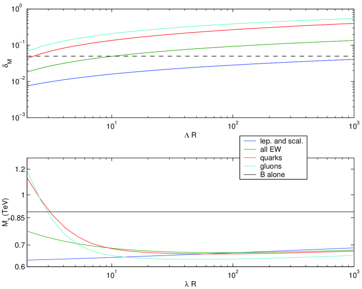
Figure 4: The calculated $\gamma^{(1)}$ mass yielding a thermal relic abundance consistent with WMAP observations is shown in the bottom graph using as a function of $\Lambda R$. This result was calculated using a simplified spectrum of the first KK level consisting of four sub-levels that vary logarithmically with $\Lambda R$, shown in the top graph. The ratios are from top to bottom: the KK gluon, the KK quarks, the KK electroweak gauge bosons, and the KK leptons and scalars, divided by the KK photon mass. The black dashed line corresponds to $\delta=0.05$ for reference. In the bottom graph, including increasing numbers of particles at the first KK level are shown with the four lines labeled in the legend. The solid straight black line (the line at the top on the far right) shows the the case without coannihilation for reference. All level one KK particles except for the leptons and scalars become rapidly irrelevant to the relic abundance calculation once $\Lambda R\gtrsim 100$.

5 Conclusions

We have calculated the thermal relic abundance of the KK photon in the five dimensional UED model for a generalized mass spectrum of level one KK particles. We find that the lowest KK photon mass which could possibly account for the observed dark matter relic abundance is $540$ GeV, resulting from including coannihilation with three generations $e_{R}$ and neutrinos all very nearly degenerate with $\gamma^{(1)}$ ($\delta=0.01$). This is consistent with the result found in Ref. [6] updated to reflect the WMAP measurements. Since the radiative mass corrections should be the same for $e_{L}$ and $\nu$, a more realistic estimate, given by including all KK leptons, is $570$ GeV. This is significantly lower than the lower mass bound of $860$ GeV given by including $\gamma^{(1)}$ alone. Including level one KK quarks and the KK gluon with masses within about 10% of the mass of the KK photon significantly increases the total effective annihilation cross section. This implies the KK photon mass leading to a thermal relic abundance consistent with WMAP observations is much larger, up to several TeV, see Figs. 2 and 4 for more precise numerical ranges. On face value, such a small separation between the KK photon and the strongly interacting level one KK particles is not expected from the radiative corrections to the masses of the first KK level computed in [5]. However, if the cutoff scale is not much larger than the KK photon mass itself, and thus matching corrections are comparable in size while opposite in sign to compensate, the level one KK spectrum could be much more degenerate. These results show that the range of the KK photon mass is much wider if indeed the mass spectrum is more degenerate than previously thought. Given measurements of the level one KK particle masses, the calculations presented here could be used to find the total effective cross section to verify if the KK photon does (or does not) make up the dark matter density needed to be consistent with WMAP observations.

Note added: During the completion of this work we became aware of an analogous calculation done independently by another group [16]. We have compared extensively the formulas for the annihilation cross-sections involving KK quarks, KK leptons and KK gauge bosons, in the limit of degenerate KK masses, as listed in the Appendix. In all considered cases we found perfect agreement.

Appendix A Universal Extra Dimensions

Here we provide a brief overview of the Universal Extra Dimension model in five dimensions (for a review, see [17]). In subsequent Appendices we list the Feynman diagrams for (co)annihilation and the cross section results we obtained. The particle content of the UED model is shown in Table 1. The $Z_{2}$ orbifold projects out one helicity of the fermion zero modes, as well as the zero mode of the $5^{th}$ component of the gauge field. We begin with a brief survey of the mass eigenstates of the theory; the Feynman rules are presented in Appendix B.

$5D$ field	$4D$ Even Fields	$4D$ Odd Fields
$A_{M}$	$A_{\mu}$	$A_{5}$
$\left(L,\tilde{L}\right)$	$L=\left(\nu,e_{L}\right)$	$\tilde{L}=\left(\nu_{R},e_{R}\right)$
$\left(Q,\tilde{Q}\right)$	$Q=\left(u_{L},d_{L}\right)$	$\tilde{Q}=\left(u_{R},d_{R}\right)$
$\left(e,\tilde{e}\right)$	$e=e_{R}$	$\tilde{e}=e_{L}$
$\left(u,\tilde{u}\right)$	$u=u_{R}$	$\tilde{u}=u_{L}$
$\left(d,\tilde{d}\right)$	$d=d_{R}$	$\tilde{d}=d_{L}$
$\phi$	$\phi$

Table 1: $5D$ fields and their behavior under the orbifold projection $y\rightarrow-y$.

A.1 Fermions

The kinetic terms for fermions have the form:

$$L_{kinetic}=\overline{\psi}(x,y)(\gamma^{\mu}\partial_{\mu}+g_{5,5}\gamma_{5}\partial_{5})\psi(x,y)$$ (12)

where we have ignored SM mass terms. Upon doing the usual Fourier expansion for, for example, the first generation of (left-handed) quarks, and integrating over $y$, we obtain:

$$L_{kinetic}= \overline{(u,d)_{L}}\gamma^{\mu}\partial_{\mu}(u,d)_{L}+\sum\limits_{j=1}^{\infty}\Big{[}\overline{P_{L}Q_{1L}^{(j)}}\left(\gamma^{\mu}\partial_{\mu}P_{L}Q_{1L}^{(j)}-\gamma^{5}\frac{j}{R}P_{R}Q_{1R}^{(j)}\right)$$ (13)

$$+\overline{P_{R}Q_{1R}^{(j)}}\left(\gamma^{\mu}\partial_{\mu}P_{R}Q_{1R}^{(j)}+\gamma^{5}\frac{j}{R}P_{L}Q_{1L}^{(j)}\right)\Big{]}\;.$$

(We use lower case letters to denote SM particles, and upper case for their KK excitations.) To obtain the full fermion masses, the usual mass terms arising from the Yukawa couplings are added (then diagonalizing the resulting mass matrices).

A.2 Gauge Bosons

After compactification, the kinetic terms in the gauge boson Lagrangian can be expressed as

$$L_{kinetic}=-\frac{1}{4}\left(F_{\mu\nu}F^{\mu\nu}+2(\partial_{5}A_{\mu}-\partial_{\mu}a)^{2}\right)$$ (14)

where $A_{\mu}$ is the 4D gauge field, and (to make the analogy with the Higgs mechanism more apparent) $a=A_{5}$, a 4D scalar. Integrating over the fifth dimension coordinate $y$ causes all cross-terms between modes of different KK-number to cancel, leaving

$$L_{kinetic}=-\frac{1}{4}\sum_{j=0}^{\infty}\left(\partial_{\mu}A^{(j)}_{\nu}-\partial_{\nu}A_{\mu}^{(j)}\right)^{2}+\frac{1}{2}\sum_{j=1}^{\infty}\left(\frac{j}{R}A_{\mu}^{(j)}-\partial_{\mu}a^{(j)}\right)^{2}\;.$$ (15)

Expanding the second term, and collecting modes of different KK number, we obtain:

$$L_{kinetic} = -\frac{1}{4}\left(\partial_{\mu}A^{(0)}_{\nu}-\partial_{\nu}A^{(0)}_{\mu}\right)^{2}+\sum\limits_{j=1}^{\infty}\bigg{[}-\frac{1}{4}\left(\partial_{\mu}A^{(j)}_{\nu}-\partial_{\nu}A^{(j)}_{\mu}\right)^{2}$$ (16)

$${}+\frac{1}{2}\left(\frac{j}{R}\right)^{2}A_{\mu}^{(j)}A^{\mu(j)}-\left(\frac{j}{R}\right)\partial_{\mu}a^{(j)}A^{\mu(j)}+\frac{1}{2}\partial_{\mu}a^{(j)}\partial^{\mu}a^{(j)}\bigg{]}$$

This is precisely the Lagrangian for a tower of 4D gauge fields with masses $M_{j}=\frac{j}{R}$ generated by a spontaneously broken symmetry. The scalar fields $a^{(j)}$ are eaten by the gauge field $A^{(j)}_{\mu}$ in the usual Higgs mechanism to give them mass.

A.3 Electroweak KK Gauge Boson Mass Eigenstates

There is a tower of KK gauge bosons for each of the SM gauge symmetries. The electroweak gauge boson KK tower, however, is different from the SM zero modes in the admixture of $W^{3(j)}$ and $B^{(j)}$. This is because the KK $SU(2)$ and $U(1)$ gauge bosons receive different loop corrections to their masses. The actual KK mass eigenstates can be found by diagonalizing the matrix

$$\left(\begin{array}[]{cc}\frac{n^{2}}{R^{2}}+\delta_{1}+\frac{1}{4}g^{2}v^{2}&\frac{1}{4}gg^{\prime}v^{2}\\ \frac{1}{4}gg^{\prime}v^{2}&\frac{n^{2}}{R^{2}}+\delta_{2}+\frac{1}{4}g^{{}^{\prime}2}v^{2}\end{array}\right)$$ (17)

where $\delta_{1}=\delta(m_{W_{3}^{(n)}})$, $\delta_{2}=\delta(m_{B^{(n)}})$ are the radiative corrections to the $n^{\rm th}$ KK level electroweak gauge bosons (precise expressions can be found in [5]). We can re-express this as:

$$\left(\begin{array}[]{cc}\frac{n^{2}}{R^{2}}+\Delta_{M}&0\\ 0&\frac{n^{2}}{R^{2}}+\Delta_{M}\end{array}\right)+\left(\begin{array}[]{cc}\delta+\frac{1}{4}g^{2}v^{2}&\frac{1}{4}gg^{\prime}v^{2}\\ \frac{1}{4}gg^{\prime}v^{2}&-\delta+\frac{1}{4}g^{{}^{\prime}2}v^{2}\end{array}\right)$$ (18)

where $\Delta_{M}=\frac{\delta_{1}+\delta_{2}}{2}$, and $\delta=\frac{\delta_{1}-\delta_{2}}{2}$. The first contribution to the masses is diagonal in the $W^{(3)}$-$B$ basis, and does not affect mixing. The mass eigenstates result from diagonalizing the second matrix; thus the Weinberg angle at each KK level is determined by the relative sizes of $\delta$ and the electroweak masses $\frac{1}{4}g_{i}g_{j}v^{2}$. Since $\delta$ is proportional to $\frac{1}{R^{2}}$, if $m_{KK}\gg M_{ew}$, the KK mass matrix is almost diagonal in the $W^{(3)}$-$B$ basis. Since $m_{KK}$ is at least 300 GeV [3], the KK Weinberg angle is much smaller than its SM counterpart. In fact, for $R^{-1}\geq 600$ GeV (which is roughly the lower bound on the mass of $B^{(1)}$) and $\Lambda/\mu\geq 2$, $\sin(\theta_{KK})<0.15$, and to the accuracy required here we can take $\gamma^{(1)}\simeq B^{(1)}$, and $Z^{(1)}\simeq W_{3}^{(1)}$.

A.4 Scalars in the Electroweak Sector

We have just shown that in the absence of other scalar interactions $A_{5}^{(n)}$ is the Goldstone boson eaten by $A_{\mu}^{(n)}$ in the effective 4D theory. In the weak sector, however, the interactions between $A_{5}$ and the KK scalar fields mix up the mass eigenstates. Note that this was also discussed in Ref. [18].

To see this, consider the 2-point vertices of the SU(2) gauge bosons. The 5D gauge field strength contributes a term of the form (16). Now we add to this the interactions with the standard model scalar fields:

$$L_{scalar} = \frac{1}{2}\left|\partial_{m}\Phi-igA_{m}^{a}T^{a}\Phi\right|^{2}$$ (19)

$$= \frac{1}{2}\Big{\{}\partial_{m}\Phi\partial^{m}\Phi+igA_{m}^{a}\left[(T^{a}\Phi)^{\dagger}\partial_{m}\Phi-\partial_{m}\Phi^{\dagger}T^{a}\Phi\right]$$

$${}\;\;+g^{2}A_{m}^{a}(T^{a}\Phi)^{\dagger}A^{m}_{b}(T^{b}\Phi)\Big{\}}$$

where $A_{m}$, $\Phi$ are the five-dimensional fields. We now will determine the physical and Goldstone scalars by examining all of the 2-point vertices in this Lagrangian.

After integrating out the $5^{th}$ dimension, and adding in the gauge boson kinetic term, the relevant piece of the Lagrangian is:

$$m_{KK}A_{\mu a}^{(n)}\partial^{\mu}a_{a}^{(n)}-\frac{1}{2}|\Phi|^{2}{m_{{{\it KK}}}}^{2}+\frac{g}{2}A^{(n)}_{\mu a}\left[T^{a}\overline{v}\partial^{\mu}\Phi^{(n)*}-\partial^{\mu}\Phi^{(n)}(T^{a}\overline{v})^{*}\right]$$

$$+\frac{g}{2}a_{a}^{(n)}\left[T^{a}\overline{v}m_{KK}\Phi^{(n)*}-m_{KK}\Phi^{(n)}(T^{a}\overline{v})^{*}\right]$$

$$+\frac{g^{2}}{2}A_{a}^{\mu(n)}A_{b\mu}^{(n)}\left[(T^{a}v)^{\dagger}T^{b}v+m_{KK}^{2}\right]-a_{a}{(n)}a_{b}^{(n)}(T^{a}v)^{\dagger}T^{b}v$$ (20)

where $\overline{v}=(0,v)$ is the standard model Higgs VEV. The terms involving $T^{a}\overline{v}\partial_{M}\Phi$ give 2-point couplings between the KK weak gauge boson and the KK excitation of the corresponding Goldstone boson, which we write as $\Phi_{a}^{(n)}$. In the case of $A_{5}^{a}(\equiv a^{a})$, these 2-point couplings involve $p_{5}\equiv m_{KK}$ rather than spatial derivatives, and thus become mass mixing terms between $\Phi^{a}$ and $a^{a}$. In addition, both $\Phi$ and $A_{\mu}^{a}$ acquire KK mass from their interactions with $a^{a}$, while $a^{a}$ gets a mass from its interactions with the Higgs VEV. Thus $a^{a}$ is no longer purely a Goldstone boson, as it has an electroweak scale mass.

A convenient gauge-fixing functional is:

$$G=\frac{1}{\sqrt{\xi}}\left[\partial^{\mu}A_{\mu a}^{(n)}-\xi(gF^{a}\Phi_{a}^{(n)}+m_{KK}a^{(n)}_{a})\right]$$ (21)

After fixing the gauge via $L\rightarrow L-\frac{1}{2}G^{2}$, all 2-point interactions between the scalars and gauge bosons of the effective 4D theory are canceled for any gauge fixing parameter $\xi$. This means that one is free to choose a gauge ($\xi\rightarrow\infty$) in which the Goldstone boson propagator vanishes. For general values of $\xi$, there are mass mixing terms between $a_{a}^{(n)}$ and $\Phi_{a}^{(n)}$. This leads to mass matrices for the scalars of the form

$$\left(\begin{array}[]{cc}m_{\it KK}^{2}\xi+m_{z}^{2}&-m_{Z}m_{\it KK}\left(\xi-1\right)\\ -m_{Z}m_{\it KK}\left(\xi-1\right)&m_{Z}^{2}\xi+m_{\it KK}^{2}\end{array}\right)$$ (22)

between $a^{a}$ and the KK excitation of the corresponding SM Goldstone boson. Here $m_{W}$ and $m_{Z}$ are the masses of the SM $W$ and $Z$ gauge bosons, respectively.

To obtain the physical and Goldstone particles, we diagonalize the mass matrix. We find the mass eigenstates

$$\rho^{(1)} = \frac{1}{\sqrt{m_{z}^{2}+m_{KK}^{2}}}(-m_{KK}a+m_{z}\Phi)\qquad\mbox{with mass}\quad\xi\sqrt{m_{KK}^{2}+m_{z}^{2}}$$

$$\rho^{(2)} = \frac{1}{\sqrt{m_{z}^{2}+m_{KK}^{2}}}(m_{z}a+m_{KK}\Phi)\;\;\>\qquad\mbox{with mass}\quad\sqrt{m_{KK}^{2}+m_{z}^{2}}$$

Clearly $\rho^{(1)}$ is the Goldstone boson, which we can be eliminated from the theory by taking the limit $\xi\rightarrow\infty$, leaving $\rho^{(2)}$ the physical scalar particle. The fact that the physical scalar is a mixture of $A_{5a}$ and $\Phi_{a}$ changes its couplings to other particles by terms proportional to the masses of the electroweak gauge bosons. Note that this mixing in the scalars is needed to ensure unitarity of gauge boson scattering is preserved, which we explicitly verified.

Since the $A_{5}$ component of the physical scalar is suppressed by $\frac{m_{Z}}{m_{KK}}$ relative to the $\Phi^{(1)}$ component, in practice this mixing can be ignored in all calculations not involving massive external SM gauge bosons.

This completes our discussion of the particle spectrum of the UED model. The KK zero modes are the particles of the Standard Model. At $n_{KK}=1$ and higher, the effective theory contains massive vector bosons that have eaten the corresponding Goldstone $A_{5}^{(n)}$ (or a combination of $A_{5}^{(n)}$ and $\Phi^{(n)}$ for the $W$ and $Z$). It also contains both helicities of SU(2) doublet and singlet fermions, with the SM helicity even under the $Z_{2}$ action, and the non-SM helicity odd. Finally, the model contains physical scalars, which are the KK Higgs, $h^{(n)}$, and $\phi^{(n)}_{W},\phi^{(n)}_{Z}$, that are mixtures of $A_{5}^{W,Z}$ with the KK excitations of the SM Goldstone bosons $\phi_{W,Z}$.

Appendix B Feynman Rules

In this section the Feynman rules relevant for the calculations used in this paper are written. Only the relevant interactions, namely between SM particles and level one KK modes, are shown. In the diagrams we use double and single lines to denote KK particles and SM particles, respectively.

B.1 Fermion/Gauge Boson Interactions

The fermion interactions of the KK modes differ from those of the standard model due to the vector-like nature of these higher modes, which introduces helicity operators at certain vertices. We find it convenient to work in unitary gauge, so that the Goldstone bosons do not appear as external particles but instead as the longitudinal polarizations of the massive KK gauge bosons. The relevant fermion interactions, after integrating over the fifth dimension, are

$$\frac{ig}{\sqrt{\pi R}}\left[\overline{f^{(0)}}\gamma^{\mu}A_{\mu}^{(1)}P_{L}F_{L}^{(1)}+\overline{P_{L}F_{L}^{(1)}}\gamma^{\mu}A_{\mu}^{(1)}f^{(0)}\right]$$ (23)

$$\frac{ig}{\sqrt{\pi R}}\left[\overline{P_{L}F^{(1)}_{L}}\gamma^{\mu}A_{\mu}^{(0)}P_{L}F_{L}^{(1)}+\overline{P_{R}F_{R}^{(1)}}\gamma^{\mu}A_{\mu}^{(0)}P_{R}F_{R}^{(1)}\right]$$ (24)

leading to the following vertices:

where $\overline{F_{L}}P_{L}F_{L}+\overline{F_{R}}P_{R}F_{R}=\overline{F}F$; i.e., this vertex is non-chiral as expected.

B.1.1 Fermion/Scalar Interactions

The interactions of fermions with scalars proportional to Yukawa couplings are presented for completeness, even though we do not make use of them since we have ignored terms of order $v^{2}/m_{KK}^{2}$. The Yukawa terms result in

$$\overline{f}^{(0)}\left[\frac{\lambda_{u}}{\sqrt{\pi R}}P_{R}G_{uR}^{(1)}i\sigma_{2}\Phi^{*(1)}+\frac{\lambda_{D}}{\sqrt{\pi R}}P_{R}G_{DR}^{(1)}\Phi^{(1)}\right]$$ (25)

$$\overline{P_{L}F_{L}^{(1)}}\left[\frac{\lambda_{u}}{\sqrt{\pi R}}P_{R}G_{uR}^{(1)}i\sigma_{2}\phi^{*}+\frac{\lambda_{D}}{\sqrt{\pi R}}P_{R}G_{DR}^{(1)}\phi\right]$$ (26)

$$\overline{P_{R}F_{R}^{(1)}}\left[\frac{\lambda_{u}}{\sqrt{\pi R}}P_{L}G_{uL}^{(1)}i\sigma_{2}\phi^{*}+\frac{\lambda_{D}}{\sqrt{\pi R}}P_{L}G_{DL}^{(1)}\phi\right]$$ (27)

$$\overline{P_{L}F_{L}^{(1)}}\left[\frac{\lambda_{u}}{\sqrt{\pi R}}g_{u}i\sigma_{2}\Phi^{*(1)}+\frac{\lambda_{D}}{\sqrt{\pi R}}g_{D}\Phi^{(1)}\right]$$ (28)

where $F$ ($f$) and $G$ ($g$) are the KK (SM) SU(2) singlet and doublet fermions, respectively. In addition, the interactions of $A_{5}$ with fermions can be deduced from the gauge boson/fermion interaction Lagrangian above. The only difference is that $A_{5}$ is odd under the orbifold $Z_{2}$, and so it couples to the “wrong” (opposite) handedness of the KK fermions. After integrating over the fifth dimension, the interaction terms become:

$$\frac{ig}{\sqrt{\pi R}}\left[\overline{f^{(0)}}\gamma^{5}A_{5}^{(1)}P_{L}F_{R}^{(1)}+\overline{P_{L}F_{R}^{(1)}}\gamma^{5}A_{5}^{(1)}f^{(0)}\right]$$ (29)

and similarly for $G$, replacing left with right KK fermions. This leads to the Feynman rules:

where $\overline{F_{L}}P_{R}G_{R}+\overline{F_{R}}P_{L}G_{L}=\overline{F}G$. Unlike the vertices between SM scalars and fermions, which are suppressed by the small Yukawa couplings, the intrinsic strength of the vertex between $A_{5}$ and fermions is not small. However, since the physical scalar particle is $m_{Z}A_{5}+m_{KK}\Phi$, in the limit that that both fermion masses and $m_{Z}$ are small compared with $m_{KK}$, we can ignore all scalar-fermion vertices.

B.1.2 Gauge Boson/Scalar Interactions

The electroweak gauge boson/scalar interactions are of the form

$$\frac{ig}{\sqrt{\pi R}}\left[A^{(0)}_{\mu}\left(\Phi\partial^{\mu}\Phi^{*}-\Phi^{*}\partial^{\mu}\Phi\right)+A^{(1)}_{\mu}\left(\phi\partial^{\mu}\Phi^{*}-\Phi^{*}\partial^{\mu}\phi+\phi^{*}\partial^{\mu}\Phi-\Phi\partial^{\mu}\phi^{*}\right)\right]+$$

$$\frac{g^{2}}{\pi R}\left[A^{(1)}_{\mu}A^{(0)\mu}\left(\Phi\phi^{*}+\Phi^{*}\phi+v\Phi+v\Phi^{*}\right)+A^{(1)}_{\mu}A^{(1)\mu}\left(|\phi|^{2}+v\phi+v\phi^{*}\right)+A^{(0)}_{\mu}A^{(0)\mu}|\Phi|^{2}\right]$$ (30)

where the gauge group indices and generators have been suppressed. The form of these interactions are nevertheless identical to those in the Standard Model.

Since $A_{5}$ and the Higgs mix with each other, as we showed above, it is convenient to compute the interactions of $A_{5}$ with electroweak gauge bosons and scalars. In the electroweak sector, where $f^{abc}=i\varepsilon^{abc}$, these interactions arise from

$$ig(\partial^{\mu}A^{a}_{5}-\partial_{5}A^{a\mu})(A^{b}_{\mu}A^{c}_{5}-A^{b}_{5}A^{c}_{\mu})-\frac{g^{2}}{2}(A^{b}_{\mu}A^{c}_{5}-A^{b}_{5}A^{c}_{\mu})^{2}\;.$$ (31)

After integrating over the fifth dimension, the only terms which survive are (using the notation $a_{k}$ to denote ${A_{5}}_{k}$):

$$\left(-\partial^{\mu}A^{a(n)}_{5}m^{(n)}_{KK}A^{a\mu(n)}\right)\left(A^{b(0)}_{\mu}A^{c(n)}_{5}-A^{b(n)}_{5}A^{c(0)}_{\mu}\right)-\frac{g^{2}}{2}(A^{b(0)}_{\mu}A^{c(n)}_{5}-A^{b(n)}_{5}A^{c(0)}_{\mu})^{2}$$ (32)

Summing over $a,b,c\in SU(2)$ and switching into the usual $W^{+},W^{-},A,Z$ basis gives the following 3-point interaction terms:

$$i\left(-{\it W^{+(n)}}_{{{\it\nu}}}{\it W^{-}}_{{\nu}}+{\it W^{-(n)}}_{{{\it\nu}}}{\it W^{+}}_{{\nu}}\right)m_{{{\it KK}}}({\it s}_{{w}}a_{{\gamma}}+c_{w}a_{{Z}})$$

$$+i\left({\it W^{+(n)}}_{{{\nu}}}(Z_{{\nu}}c_{{w}}+A_{{\nu}}{\it s}_{{w}})-(A^{(n)}_{{{\nu}}}{\it s}_{{w}}+Z^{(n)}_{{{\nu}}}c_{{w}}){\it W^{+}}_{{\nu}}\right)m_{{{\it KK}}}a_{{-}}$$

$$+i\left(-{\it W^{-(n)}}_{{{\nu}}}(Z_{{\nu}}c_{{w}}+A_{{\nu}}{\it s}_{{w}})+(Z^{(n)}_{{{\nu}}}c_{{w}}+A^{(n)}_{{{\nu}}}{\it s}_{{w}}){\it W^{-}}_{{\nu}}\right)m_{{{\it KK}}}a_{{+}}$$ (33)

for the two gauge boson/$A_{5}$ interactions, and

$$-i\left(a_{{-}}^{(n)}{\partial}a_{{+}}^{(n)}-a^{(n)}_{{+}}{\partial}a_{{-}}^{(n)}\right){\it s}_{w}A^{(0)}_{{\nu}}-i\left(-a_{{+}}^{(n)}{\partial}a_{{-}}+a_{{-}}^{(n)}{\partial}a_{{+}}^{(n)}\right)c_{w}Z_{{\nu}}^{(0)}$$

$$-i\left(\left\{a_{{z}}^{(n)}c_{{w}}+a_{{\gamma}}^{(n)}{\it s}_{{w}}\right\}{\partial}a_{{-}}^{(n)}-a_{{-}}^{(n)}\left\{{\partial}a_{{\gamma}}^{(n)}{\it s}_{{w}}{\partial}a_{{z}}^{(n)}c_{{w}}\right\}\right){\it W^{+(0)}}_{{\nu}}-$$

$$i\left(-\left\{a_{{z}}^{(n)}c_{{w}}+a_{{\gamma}}^{(n)}{\it s}_{{w}}\right\}{\partial}a_{{+}}^{(n)}+a_{{+}}^{(n)}\left\{{\partial}a_{{\gamma}}^{(n)}{\it s}_{{w}}+{\partial}a_{{z}}^{(n)}c_{{w}}\right\}\right){\it W^{-(0)}}_{{\nu}}$$ (34)

for the triple-scalar/gauge boson interactions. The 4-point interactions are obtained from the corresponding standard model vertices by requiring both KK particles be $A_{5}$.

$A_{5}$ also couples to $\Phi$ through $|D_{\mu}\Phi|^{2}$. This results in three types of vertices: $V_{1}=gm_{KK}A_{5}\Phi\Phi^{*}$, $V_{2}=gm_{Z}A_{5}A_{5}\Phi$, and $V_{3}=g^{2}A_{5}A_{5}\Phi\Phi^{*}$. $V_{2}$ and $V_{3}$ are identical to those of the KK gauge bosons, once the factors of $g_{\mu\nu}$ are replaced with $g_{55}$. $V_{1}$ is obtained from the corresponding KK gauge boson vertex by replacing $p_{\mu}\rightarrow im_{KK}$. As some care must be taken with signs, the $V_{1}$ terms are listed here:

$$-i{\it s}_{{w}}\left(-{w_{{+}}}^{(n)}w_{{-}}+{w_{{-}}}^{(n)}w_{{+}}\right)a_{{\gamma}}^{(n)}$$

$$+\frac{1}{2\cos\left(\theta_{w}\right)}\,a_{{z}}^{(n)}\left(\,i\cos\left(2\theta_{w}\right)({w_{{+}}}^{(n)}w_{{-}}-{w_{{-}}}^{(n)}w_{{+}})+{h}^{(n)}z-{z}^{(n)}h\right)$$

$$+\frac{1}{2}\,\left(-iz{w_{{+}}}^{(n)}-h{w_{{+}}}^{(n)}+{h}^{(n)}w_{{+}}+i{z}^{(n)}w_{{+}}\right)a_{{-}}$$

$$+\frac{1}{2}\,\left(iz{w_{{-}}}^{(n)}-h{w_{{-}}}^{(n)}+{h}^{(n)}w_{{-}}-i{z}^{(n)}w_{{-}}\right)a_{{+}}$$ (35)

The vertices involving physical scalars follow from combining vertices involving $A_{5}$ and $\Phi$ in the correct proportion. A table of these physical vertices is given below. In principle, care must be taken in vertices involving the Weinberg angle, as the mass mixing is not the same for the $KK$ particles as it is for the SM particles. In the case of the scalar $A_{5}$, however, the physical component of $A_{5}$ is that which mixes with the SM Goldstone boson of the $Z$ particle, and hence its mixing angle should be the same as that of the SM $Z$ boson. For the KK gauge bosons, the mixing angle is different. However, as we already discussed above, it is a good approximation to neglect this mixing and thus take $\gamma^{(1)}\simeq B^{(1)}$ and $Z^{(1)}\simeq W^{3(1)}$.

The following notation is used in the table. We define $\kappa_{w}=\frac{m_{KK}}{\sqrt{m_{KK}^{2}+m_{W}^{2}}}$ and $\kappa_{z}=\frac{m_{KK}}{\sqrt{m_{KK}^{2}+m_{Z}^{2}}}$. $\Phi_{z},\Phi_{+}$, and $\Phi_{-}$ are the physical level one KK scalars that are themselves mixtures of the KK excitations of the SM Goldstone bosons and $A_{5}$ from the weak gauge bosons, as described in Sec. A.4. (Here we use level one KK particles, but the vertices are the same for level $n$ KK states also.). $\Phi_{h}$ is the level one KK Higgs particle, while $h$ is the SM Higgs particle. The table includes only vertices which differ from those of the SM.

2 vector/scalar vertices
Vertex	Coupling
$W^{+(1)}_{\mu}W^{-(0)}_{\nu}\Phi_{z}$	$-ic_{w}(-1)^{\beta}m_{z}\kappa_{z}g_{\mu\nu}$
$W^{-(1)}_{\mu}W^{+(0)}_{\nu}\Phi_{z}$	$ic_{w}(-1)^{\beta}m_{z}\kappa_{z}g_{\mu\nu}$
$W^{+(1)}_{\mu}Z^{(0)}_{\nu}\Phi_{-}$	$im_{Z}(s_{w}^{2}+(-1)^{\beta}c_{w}^{2})\kappa_{w}g_{\mu\nu}$
$W^{-(1)}_{\mu}Z^{(0)}_{\nu}\Phi_{+}$	$-im_{Z}(s_{w}^{2}+(-1)^{\beta}c_{w}^{2})\kappa_{w}g_{\mu\nu}$
$W^{-(0)}_{\mu}Z^{(1)}_{\nu}\Phi_{+}$	$-im_{Z}(s_{w}^{2}-(-1)^{\beta}c_{w}^{2})\kappa_{w}g_{\mu\nu}$
$W^{+(0)}_{\mu}Z^{(1)}_{\nu}\Phi_{-}$	$im_{Z}(s_{w}^{2}-(-1)^{\beta}c_{w}^{2})\kappa_{w}g_{\mu\nu}$
$W^{+(1)}_{\mu}A^{(0)}_{\nu}\Phi_{-}$	$\frac{1}{2}im_{Z}\sin(2\theta_{w})((-1)^{\beta}-1)\kappa_{w}g_{\mu\nu}$
$W^{-(1)}_{\mu}A^{(0)}_{\nu}\Phi_{+}$	$\frac{-1}{2}im_{Z}\sin(2\theta_{w})((-1)^{\beta}-1)\kappa_{w}g_{\mu\nu}$
$W^{-(0)}_{\mu}A^{(1)}_{\nu}\Phi_{+}$	$\frac{1}{2}im_{Z}\sin(2\theta_{w})((-1)^{\beta}+1)\kappa_{w}g_{\mu\nu}$
$W^{+(0)}_{\mu}A^{(1)}_{\nu}\Phi_{-}$	$\frac{-1}{2}im_{Z}\sin(2\theta_{w})((-1)^{\beta}-1)\kappa_{w}g_{\mu\nu}$
$A_{\mu}^{(i)}A_{\nu}^{(j)}\Phi_{h}$	as in standard model

2 scalar/vector vertices
Vertex	Coupling
$A_{\mu}^{(0)}\Phi_{+}\Phi_{-}$	$gs_{w}(p_{+}-p_{-})$
$Z_{\mu}^{(0)}\Phi_{+}\Phi_{-}$	$g(c_{w}-\frac{cos(2\theta_{W})}{2c_{w}}\kappa_{w}^{2})(p_{+}-p_{-})$
$W_{\mu}^{+(0)}\Phi_{z}\Phi_{-}$	$g\left(\frac{m_{W}^{2}}{m_{KK}^{2}}+\frac{1}{2}\right)\kappa_{z}\kappa_{w}(p_{-}-p_{z})$
$W_{\mu}^{-(0)}\Phi_{z}\Phi_{+}$	$-g\left(\frac{m_{W}^{2}}{m_{KK}^{2}}+\frac{1}{2}\right)\kappa_{z}\kappa_{w}(p_{+}-p_{z})$
$A_{\mu}^{(0)j}\Phi_{j}\Phi_{h}$	$\kappa_{j}\times$ SM vertex

2 vector/2 scalar vertices
$W^{+(0)}_{\mu}W^{-(0)}_{\nu}\Phi_{+}\Phi_{-}$	$\frac{g^{2}}{2}(1+\frac{2m_{W}^{2}}{m_{KK}^{2}})\kappa_{w}^{2}g_{\mu\nu}$
$W^{+(0)}_{\mu}W^{-(0)}_{\nu}\Phi_{z}\Phi_{z}$	$\frac{g^{2}}{2}\kappa_{z}^{2}(1+4\frac{c_{w}^{2}m_{Z}^{2}}{m_{KK}^{2}})g_{\mu\nu}$
$A^{(0)}_{\mu}A^{-(0)}_{\nu}\Phi_{+}\Phi_{-}$	$2e^{2}g_{\mu\nu}$
$Z^{(0)}_{\mu}Z^{(0)}_{\nu}\Phi_{+}\Phi_{-}$	$g^{2}\kappa_{w}^{2}(\frac{\cos(2\theta_{w})^{2}}{2c_{w}^{2}}+\frac{2c_{w}^{4}m_{Z}^{2}}{m_{KK}^{2}})g_{\mu\nu}$
$Z^{(0)}_{\mu}A^{(0)}_{\nu}\Phi_{+}\Phi_{-}$	$ge\kappa_{w}^{2}(\frac{\cos(2\theta_{w})}{c_{w}}+\frac{2c_{w}^{3}m_{Z}^{2}}{m_{KK}^{2}})g_{\mu\nu}$
$Z^{(0)}_{\mu}W^{\pm(0)}_{\nu}\Phi_{z}\Phi_{\pm}$	$\frac{g^{2}}{2}\kappa_{w}\kappa_{z}(\frac{s_{w}^{2}}{c_{w}}-\frac{c_{w}^{3}m_{Z}^{2}}{m_{KK}^{2}})g_{\mu\nu}$
$A^{(0)}_{\mu}W^{\pm(0)}_{\nu}\Phi_{z}\Phi_{\pm}$	$\frac{-ge}{2}\kappa_{w}\kappa_{z}(1+\frac{c_{w}^{2}m_{Z}^{2}}{m_{KK}^{2}})g_{\mu\nu}$

3 scalar vertices
$\Phi_{z}\Phi_{z}h$	$-(m_{Z}^{2}(1+\frac{m_{Z}^{2}}{m_{KK}^{2}})+\frac{1}{2}M_{h}^{2})\frac{\kappa_{z}^{2}}{c_{w}m_{Z}}$
$\Phi_{w}\Phi_{w}h$	$-(m_{W}^{2}(1+\frac{m_{W}^{2}}{m_{KK}^{2}})+\frac{1}{2}M_{h}^{2})\frac{\kappa_{w}^{2}}{c_{w}m_{Z}}$
4 scalar vertices
$\Phi_{+}\Phi_{-}hh$	$\frac{-g^{2}\kappa_{w}^{2}}{4}(\frac{M_{h}^{2}}{m_{W}^{2}}+2\frac{m_{W}^{2}}{m_{KK}^{2}})$
$\Phi_{z}\Phi_{z}hh$	$\frac{-g^{2}\kappa_{z}^{2}}{4c_{w}^{2}}(\frac{M_{h}^{2}}{m_{Z}^{2}}+2\frac{m_{Z}^{2}}{m_{KK}^{2}})$

Here we have included only vertices in which the SM scalars are the physical Higgs particle. In practice, to lowest order in $v/m_{KK}$, the only vertices that are affected are those whose analogue in the SM contains a factor of $m_{Z}$. In this case, the contributions of certain $A_{5}$ terms can be of the same order in $m_{Z}$ as the contributions of $\Phi^{(1)}$.

Note that vertices of the form $A^{\mu a}A^{b}_{\mu}a^{c}$ have a sign which depends on whether the indices $a,b,c$ occur in clockwise or counter-clockwise order, caused by $\varepsilon^{abc}$ from the commutators of $SU(2)$ generators. Diagrams of the form $A^{a\mu}A^{a}_{\mu}\Phi$, have no such sign. Hence care must be taken in combining the contributions of these two types of diagrams to obtain the physical scalar vertex. In order to make this clear, we have explicitly kept a factor of $(-1)^{\beta}$ in the relevant vertices. Here $\beta$ is even for vertices in which the electric charge entering the vertex increases in the counter-clockwise direction, and is odd otherwise.

The gauge boson self-interaction terms are exactly as in the standard model, and need not be reviewed here. Note that $A^{(1)}_{\mu}$, being even under orbifold parity, has no vertices with the Goldstone boson $A_{5}$ apart from those in the kinetic terms described above.

Appendix C Generic Diagrams and their annihilation cross sections

In this section, we list all Feynman diagrams involved in the annihilation processes we consider. (As explained above, processes involving the Yukawa coupling of Higgs to fermions, the self-coupling of Higgs to itself, are not calculated as they are expected to have a small effect on these results.) The possible annihilation processes are classified according to the nature of the initial and final state particles. Some diagrams apply to multiple processes, and not all diagrams in a given section necessarily apply to all processes of that type. A comprehensive list of processes, the relevant diagrams, and the corresponding cross sections can be found in Appendix D.

C.1 Fermion Annihilation

C.1.1 $f^{(1)}f^{(1)}\rightarrow f^{(0)}f^{(0)}$ and $f^{(1)}\overline{f}^{(1)}\rightarrow f^{(0)}\overline{f}^{(0)}$

C.1.2 $f^{(1)}\overline{f}^{(1)}\rightarrow A_{\mu}^{(0)}A_{\nu}^{(0)}$

Here the set of diagrams depends on the particular final state; i.e., the last diagram is absent when the final state gauge bosons are hypercharge.

C.1.3 $f^{(1)}\overline{f}^{(1)}\rightarrow\phi^{(0)}\phi^{*(0)}$

C.2 Gauge Boson Annihilation

C.2.1 $A_{\mu}^{(1)}A_{\nu}^{(1)}\rightarrow f^{(0)}\overline{f}^{(0)}$

Here vertices involving both SM and KK fermions are chiral, as previously mentioned, and factors of the appropriate helicity projection operators must be included. In the limit that electroweak breaking masses are ignored, all of these scattering processes result in two final state fermions of the same chirality.

C.2.2 $W_{\mu}^{(1)}W_{\nu}^{(1)}\rightarrow\phi^{(0)}\phi^{*(0)}$ and $Z_{\mu}^{(1)}Z_{\nu}^{(1)}\rightarrow\phi^{(0)}\phi^{*(0)}$

This set of diagrams corresponds to the annihilation of $W$ or $Z$ bosons into at least one physical SM Higgs boson. In the limit that the masses of the SM $W$ and $Z$ are small compared to $s$, we can consistently ignore diagrams with vertices of the form $WW\phi$, $ZZ\phi$, and $WZ\phi$, as their couplings are suppressed by $v/m_{KK}$ or $v^{2}/s$. If one of the external particles is a gauge boson, the Goldstone boson equivalence theorem tells us that only the longitudinal polarization of the external gauge boson contributes. We can then use the Goldstone boson approximation to calculate the relevant cross sections from the set of diagrams below.

C.2.3 $A_{\mu}^{(1)}A_{\nu}^{(1)}\rightarrow A_{\mu}^{(0)}A_{\nu}^{(0)}$

This set of diagrams corresponds to KK gauge boson annihilation into SM gauge bosons. Note that we treated SM electroweak gauge bosons as massive, so that no external Goldstone bosons are necessary. However, all diagrams with physical scalar propagators must be included. In the $s$-channel, only the Higgs plays a role. However, since there are physical KK $w$ and $z$ scalars, these propagators must be included in the $t$ and $u$ channels. We remark that would-be high-energy divergences of the form $s/m_{KK}^{2}$ are absent precisely because the the non-Goldstone scalars are a mixture of $\phi^{(1)}$ and $A_{5}^{(1)}$.

C.3 Higgs Annihilation

C.3.1 $\Phi^{(1)}\Phi^{(1)}\rightarrow\phi^{(0)}\phi^{(0)}$

This set of diagrams correspond to scalar annihilation into at least one final state Higgs particle. If final state gauge bosons are present, the resulting diagrams contain at least one coupling proportional to $m_{Z}$, and hence are highly suppressed unless the gauge boson is longitudinally polarized. Thus all such processes can be described by purely scalar final states in the limit that we ignore terms proportional to $m_{Z}/m_{KK}$.

Here we furthermore ignore diagrams involving 3-scalar vertices, since their contribution is suppressed by factors of $v/m_{KK}$ or $v^{2}/s$.

C.3.2 $\Phi^{(1)}\Phi^{*(1)}\rightarrow A_{\mu}^{(0)}A_{\nu}^{(0)}$

C.3.3 $\Phi^{(1)}\Phi^{*(1)}\rightarrow f^{(0)}\overline{f}^{(0)}$

C.4 Fermion/gauge boson coannihilation

C.4.1 $f^{(1)}A_{\nu}^{(1)}\rightarrow f^{(0)}A_{\nu}^{(0)}$

C.5 Gauge boson/Higgs coannihilation

C.5.1 $\Phi^{(1)}A_{\nu}^{(1)}\rightarrow\Phi^{(0)}A_{\nu}^{(0)}$

Here again we work in the limit $m_{W}\ll s,m_{KK}$. In this limit, processes to two final state scalars can be neglected, as they necessarily involve at least one vertex suppressed by a factor of $m_{Z}$. In processes to one final state scalar and one final state gauge boson, diagrams in which scalar propagators are replaced by gauge boson propagators are also electroweak suppressed (by $m_{Z}^{2}$, while the longitudinal gauge boson contributes $1/m_{Z}$) and thus neglected.

C.6 Fermion/Higgs Coannihilation

C.6.1 $\Phi^{(1)}f^{(1)}\rightarrow\Phi^{(0)}f^{(0)}$

This coannihilation diagram includes processes to external Goldstone bosons which are of course just the leading order contribution to the analogous process of coannihilating into external SM gauge bosons.

Appendix D Cross Sections

D.1 Fermion Annihilation

The following sections refer to the diagrams and matrix elements computed in Sec. C, by the Section numbers assigned to each process. The total cross section is the sum of the appropriate terms and cross-terms, multiplied by the necessary spin averaging and identical particle factors. We use the notation $L=\ln\left(\frac{1+\beta}{1-\beta}\right)$.

D.1.1 $e_{R}$

Process	Diagrams	Total cross section
$E_{R}E_{R}\rightarrow e_{R}e_{R}$	C.1.1 a,b	$\frac{g_{1}^{4}Y_{e_{R}}^{4}}{32\pi\beta^{2}s^{2}m_{KK}^{2}}[\beta s(2s-m_{KK}^{2})+m_{KK}^{2}(4s-5m_{KK}^{2})L]$
$E_{R}\overline{E_{R}}\rightarrow e\overline{e}$	C.1.1 c,d	$\frac{g_{1}^{4}Y_{e_{R}}^{4}}{192\pi\beta^{2}s^{2}}[\beta(12s^{2}+16m_{KK}^{4}+65sm_{KK}^{2})-12m_{KK}^{2}(4s+3m_{KK}^{2})L]$
		$+\frac{g_{1}^{4}Y_{e_{R}}^{2}Y_{e_{L}}^{2}}{24\pi\beta s^{2}}(s+2m_{KK}^{2})$
$E_{R}\overline{E_{R}}\rightarrow f\overline{f}$	C.1.1 d	$\frac{g_{1}^{4}Y_{e_{R}}^{2}(s+2m_{KK}^{2})}{24\pi\beta s^{2}}\sum_{f=\neq e}Nc(Y_{f_{R}}^{2}+Y_{f_{L}}^{2})$
$E_{R}\overline{\mu_{R}}\rightarrow e_{R}\overline{\mu_{R}}$	C.1.1 c	$\frac{g_{1}^{4}Y_{e_{R}}^{4}}{64\pi\beta^{2}sm_{KK}^{2}}[\beta(4s+9m_{KK}^{2})-8m_{KK}^{2}L]$
$E_{R}\mu_{R}\rightarrow e_{R}\mu_{R}$	C.1.1 a	$\frac{g_{1}^{4}Y_{e_{R}}^{4}}{64\pi\beta sm_{KK}^{2}}(4s-3m_{KK}^{2})$
$E_{R}\overline{E_{R}}\rightarrow\phi\phi^{*}$	C.1.3	$\frac{g_{Ze}^{2}g_{Z\phi}^{2}}{48\pi\beta s^{2}}(s+2m_{KK}^{2})$
$E_{R}\overline{E_{R}}\rightarrow\gamma\gamma$	C.1.2 a,b	$\frac{e^{4}}{8\pi s^{3}\beta^{2}}\left\{(s^{2}+4m_{KK}^{2}s-8m_{KK}^{4})L-s\beta(s+4m_{KK}^{2})\right\}$
$E_{R}\overline{E_{R}}\rightarrow ZZ$	C.1.2 a,b	$\frac{g^{4}\left(\frac{2(-1/2+\sin(\theta_{W}))}{sin(2\theta_{W}}\right)^{4}}{8\pi s^{3}\beta^{2}}\left\{(s^{2}+4m_{KK}^{2}s-8m_{KK}^{4})L-s\beta(s+4m_{KK}^{2})\right\}$
$E_{R}\overline{E_{R}}\rightarrow WW$	C.1.2 c	$\,{\frac{e^{4}(s+2\,{{\it m_{KK}}}^{2})}{192\pi\,{s}^{2}\beta\,{c_{{w}}}^{4}}}$

Note that in the $s$-channel diagrams the mass of the propagator was ignored (i.e., only hypercharge gauge photon exchanged), since we neglected terms of order $v^{2}/m_{KK}^{2}$.

D.1.2 $e_{L}$

Process	Diagrams	Total cross section
$E_{L}\overline{E_{L}}\rightarrow e^{\prime}_{L}\overline{e^{\prime}_{L}}$	C.1.1 c,d	$\frac{g_{s}^{2}g_{t,e}^{2}[5\,s\beta-2\,\left(2\,s+3\,{m_{{{\it KK}}}}^{2}\right)L]}{32\pi s^{2}\beta^{2}}+{\frac{g_{t,e}^{4}[\beta\,\left(4\,s+9\,{m_{{{\it KK}}}}^{2}\right)-8\,{m_{{{\it KK}}}}^{2}L]}{64\pi s\beta^{2}m_{\it KK}^{2}}}$
		$+{\frac{g_{s}^{4}[s+2\,{m_{{{\it KK}}}}^{2}]}{24\pi s^{2}\beta}}$
$E_{L}\overline{E_{L}}\rightarrow W^{+}W^{-}$	C.1.2 a,c	$\,g^{4}{\frac{\left(96\,{c_{{w}}}^{4}{m_{{{\it KK}}}}^{2}+24\,s{c_{{w}}}^{4}\right)L+2\,\beta\,{m_{{{\it KK}}}}^{2}+s\beta-40\,s{c_{{w}}}^{4}\beta-176\,\beta\,{m_{{{\it KK}}}}^{2}{c_{{w}}}^{4}}{768\pi\,{s}^{2}{\beta}^{2}{c_{{w}}}^{4}}}$

Cross sections identical in nature to those of $E_{R}$ have not been reproduced in this table. They can be obtained from the previous table with appropriate replacements of the coupling constants.

In the cross section to leptons of the same generation, explicit coupling factors have been kept since the diagrams are the same for both (i) $E_{L}\overline{E_{L}}\rightarrow e_{L}\overline{e_{L}}$ and (ii) $E_{L}\overline{E_{L}}\rightarrow\nu_{e}\overline{\nu_{e}}$, as well as the analogous processes with neutrinos in the initial state (iii) and (iv). Here $g^{2}_{s(t)}$ is the total coupling in the $s$-($t$-)channel. Ignoring the SM gauge boson masses, $g_{s}^{2}=g_{t}^{2}=g^{2}(\tan^{2}\theta_{W}Y_{E_{L}}Y_{e_{L}}+T_{3}(E_{L})T_{3}(e_{L}))$ for annihilation into the same particle, and $g_{s}^{2}=g^{2}(\tan^{2}\theta_{W}Y_{E_{L}}Y_{\nu_{L}}+T_{3}(E_{L})T_{3}(\nu_{L}))$ $g_{t}^{2}=g^{2}/2$ for processes to the electroweak partner (where the $t$-channel is mediated by a $W^{\pm}$ boson).

For cross sections to gauge bosons, the leading terms in the limit of vanishing gauge boson mass have been kept.

D.1.3 quarks

The processes $QQ\rightarrow qq$ and $Q\overline{Q}\rightarrow q\overline{q}$ are essentially the same as the corresponding processes for electrons shown above, except that an additional diagram involving gluon exchange is present. In the limit that all KK gauge bosons have mass, and we ignore the masses of all SM gauge bosons in the $s$ channel, the relevant amplitude comes from the electron amplitude (with the appropriate modification of the hypercharge value) plus the same amplitude with all couplings changed to $g_{s}$. Annihilation to scalars and electroweak gauge bosons are identical to the electron case, with the appropriate couplings. Thus the only novel diagrams are annihilation to $gg$ and $g\gamma$.

Process	Diagrams	Total cross section
$Q\overline{Q}\rightarrow g\gamma$	C.1.2 a,b	$\frac{e^{2}g_{s}^{2}}{2}\,{\frac{\left(-8\,{m_{{{\it KK}}}}^{4}+4\,{m_{{{\it KK}}}}^{2}s+{s}^{2}\right)L-{s}^{2}\beta-4\,\beta\,{m_{{{\it KK}}}}^{2}s}{18\pi\,{s}^{3}{\beta}^{2}}}$
$Q\overline{Q}\rightarrow gZ$	C.1.2 a	$\frac{g_{s}^{2}g_{Z,q}^{2}}{36}\,{\frac{\left({s}^{2}+4\,s{m_{{{\it KK}}}}^{2}-8\,{m_{{{\it KK}}}}^{4}\right)L-{s}^{2}\beta-4\,s\beta\,{m_{{{\it KK}}}}^{2}}{{\beta}^{2}{s}^{3}\pi}}$
$Q\overline{Q}\rightarrow gg$	C.1.2 a,b,c	$-\frac{g_{s}^{4}}{216}{\frac{-4\,\left({m_{KK}}^{4}+4\,s{m_{KK}}^{2}+\,{s}^{2}\right)L+7\,\beta\,{s}^{2}+31\,s\beta\,{m_{KK}}^{2}}{\pi{s}^{3}{\beta}^{2}}}$

Here $g_{Z,q}$ is the coupling of the quark to the Z boson. Note that in annihilation to gluons, the appropriate color factors have been included, along with a factor of $\frac{1}{9}$ for the average over quark colors. In $qq\rightarrow g\gamma$ or $qq\rightarrow gZ$, a factor of $1/2$ must be included for the trace over $t^{a}t^{b}$.

D.2 Gauge Boson Annihilation

Because the KK Weinberg angle is sufficiently small that its effect on our computations can be neglected, the results here are presented in the $B^{(1)}$, $W^{3(1)}$ basis.

D.2.1 Hypercharge

Process	Diagrams	Total cross section
$B_{\mu}B_{\nu}\rightarrow f\overline{f}$	C.2.1 a,b	$\,{\frac{g_{1}^{4}Y_{f}^{4}[(10\,{m_{{{\it KK}}}}^{2}+5\,s)L-7\,s\beta]}{72{s}^{2}\pi\,{\beta}^{2}}}$
$B_{\mu}B_{\nu}\rightarrow W^{+}W^{-}$	C.2.3 d,e,f	${\frac{1}{192}}\,{\frac{{{\it s}_{{w}}}^{4}{g}^{4}}{\beta\,{c_{{w}}}^{4}\pi\,s}}$
$B_{\mu}B_{\nu}\rightarrow ZZ$	C.2.3 d,e,f	$\frac{1}{2}{\frac{1}{192}}\,{\frac{{{\it s}_{{w}}}^{4}{g}^{4}}{\beta\,{c_{{w}}}^{4}\pi\,s}}$
$B_{\mu}B_{\nu}\rightarrow hh$	C.2.2 a,b,c	$\frac{1}{2}{\frac{1}{192}}\,{\frac{{{\it s}_{{w}}}^{4}{g}^{4}}{\beta\,{c_{{w}}}^{4}\pi\,s}}$

D.3 $W_{3}$

Process	Diagrams	Total cross section
$W_{3\mu}W_{3\nu}\rightarrow f\overline{f}$	C.2.1 a,b	$\,{\frac{g^{4}T_{3}(f)^{4}[(10\,{m_{{{\it KK}}}}^{2}+5\,s)L-7\,s\beta]}{72{s}^{2}\pi\,{\beta}^{2}}}$
$W_{3\mu}W_{3\nu}\rightarrow\phi\phi$	C.2.2 a,b,c	${\frac{1}{2}\frac{g^{4}}{192\pi\,s\beta}}$
$W_{3\mu}W_{3\nu}\rightarrow Z_{\mu}Z_{\nu}$	C.2.3 d,e,f	$\frac{1}{2}{\frac{g^{4}}{192\beta\,\pi\,s}}$
$W_{3\mu}W_{3\nu}\rightarrow W^{+}W^{-}$	C.2.3 a,b,c,d,e,f	$\frac{{g}^{4}}{18}\,{\frac{\left(-12\,{m_{{{\it KK}}}}^{4}s+24\,{m_{{{\it KK}}}}^{6}\right)L+4\,\beta\,{s}^{3}+3\,\beta\,{m_{{{\it KK}}}}^{2}{s}^{2}+12\,s{m_{{{\it KK}}}}^{4}\beta}{\pi\,{s}^{3}{\beta}^{2}{m_{{{\it KK}}}}^{2}}}$
		$+{\frac{1}{192}}\,{\frac{{g}^{4}}{\beta\,\pi\,s}}$

D.4 $W^{\pm}$

Process	Diagrams	Total cross section
$W^{+}_{\mu}W^{-}_{\nu}\rightarrow f_{R}\overline{f_{R}}$	C.2.1 c	0 to leading order in the SM z boson mass
$W^{+}_{\mu}W^{-}_{\nu}\rightarrow f_{L}\overline{f_{L}}$	C.2.1 a,c	${\frac{g^{4}}{8}}\,{\frac{\left(5\,s+12\,{m_{{{\it KK}}}}^{2}\right)L-10\,\beta\,s-8\,\beta\,{m_{{{\it KK}}}}^{2}}{72\pi\,{s}^{2}{\beta}^{2}}}$
$W^{+}_{\mu}W^{-}_{\nu}\rightarrow W^{+}_{\nu}W^{-}_{\mu}$	C.2.3 a,c,d,e,s	$\,\frac{g^{4}}{144}{\frac{\left(-32\,{m_{{{\it KK}}}}^{2}s-48\,{m_{{{\it KK}}}}^{4}\right)L+16\,{s}^{2}\beta+41\,{m_{{{\it KK}}}}^{2}\beta\,s+87\,{m_{{{\it KK}}}}^{4}\beta}{\pi\,{s}^{2}{\beta}^{2}{m_{{{\it KK}}}}^{2}}}$
$W^{+}_{\mu}W^{-}_{\nu}\rightarrow A_{\nu}A_{\mu}$	C.2.3 a,b,c	$\,\frac{e^{4}}{2}{\frac{\left(-12\,{m_{{{\it KK}}}}^{4}s+24\,{m_{{{\it KK}}}}^{6}\right)L+4\,\beta\,{s}^{3}+3\,\beta\,{m_{{{\it KK}}}}^{2}{s}^{2}+12\,{m_{{{\it KK}}}}^{4}s\beta}{18\pi\,{\beta}^{2}{m_{{{\it KK}}}}^{2}{s}^{3}}}$
$W^{+}_{\mu}W^{-}_{\nu}\rightarrow Z_{\nu}Z_{\mu}$	C.2.3 a,b,c,d,e,f	$\,{\frac{{g^{4}c_{{w}}}^{4}\left(24\,L{m_{{{\it KK}}}}^{6}+12\,{m_{{{\it KK}}}}^{4}s\beta-12\,L{m_{{{\it KK}}}}^{4}s+3\,{s}^{2}\beta\,{m_{{{\it KK}}}}^{2}+4\,{s}^{3}\beta\right)}{36\pi\,{s}^{3}{\beta}^{2}{m_{{{\it KK}}}}^{2}}}$
		$+{\frac{1}{384}}\,{\frac{{g}^{4}}{\beta\,\pi\,s}}$
$W^{+}_{\mu}W^{-}_{\nu}\rightarrow Z_{\nu}A_{\mu}$	C.2.3 a,b,c	$\frac{e^{2}c_{w}^{2}g^{2}}{18}{\frac{\left(-12\,{m_{{{\it KK}}}}^{4}s+24\,{m_{{{\it KK}}}}^{6}\right)L+4\,\beta\,{s}^{3}+3\,\beta\,{m_{{{\it KK}}}}^{2}{s}^{2}+12\,s\beta\,{m_{{{\it KK}}}}^{4}}{\pi\,{s}^{3}{\beta}^{2}{m_{{{\it KK}}}}^{2}}}$
$W^{+}_{\mu}W^{-}_{\nu}\rightarrow hh$	2.2.3 a,b,c	${\frac{1}{2}\frac{g^{4}}{192\pi\,s\beta}}$
$W^{+}_{\mu}W^{-}_{\nu}\rightarrow hz$	2.2.3 a,b,d	${\frac{g^{4}}{576}}\,{\frac{s-4\,{m_{{{\it KK}}}}^{2}}{\pi\,{s}^{2}\beta}}$

D.5 Gluon

Process	Diagrams	Total cross section
$g_{\mu}g_{\nu}\rightarrow f\overline{f}$	C.2.1 a,b,c	${\frac{g_{s}^{4}}{64}}\,{\frac{\left(40\,s+98\,{m_{{{\it KK}}}}^{2}\right)L-83\,\beta\,s-72\,\beta\,{m_{{{\it KK}}}}^{2}}{6\pi\,{s}^{2}{\beta}^{2}}}$
$g_{\mu}g_{\nu}\rightarrow g_{\nu}g_{\mu}$	C.2.3 a,b,c,s	$\,{g_{s}^{4}\frac{\left(-8\,{m_{{{\it KK}}}}^{2}{s}^{2}-24\,{m_{{{\it KK}}}}^{4}s+24\,{m_{{{\it KK}}}}^{6}\right)L+8\,{s}^{3}\beta+13\,{m_{{{\it KK}}}}^{2}\beta\,{s}^{2}+34\,{m_{{{\it KK}}}}^{4}s\beta}{32\pi\,{s}^{3}{\beta}^{2}{m_{{{\it KK}}}}^{2}}}$

Here the factor of $1/64$ was included for the average over initial gluon colors.

D.6 Scalar Annihilation

In this set of cross sections, note that the KK modes of the SM Goldstone bosons are in fact separate propagating degrees of freedom, and thus their annihilation cross sections must be calculated independently of those of the KK W and Z bosons. For processes to one Higgs and one SM gauge bosons, we use the Goldstone boson approximation, as processes to final state transverse polarizations are suppressed by $v/m_{KK}$.

Scalar Annihilation into Scalars:
Process	Diagrams	Total cross section
$w^{+}w^{-}\rightarrow hh$	C.3.1 a,b,d	$\,{\frac{{H}^{2}}{512\pi\,s\beta\,{c_{{w}}}^{4}}}+\,{\frac{\left(4\,\beta\,{m_{{{\it KK}}}}^{2}-8\,{m_{{{\it KK}}}}^{2}L\right)H}{512\pi\,{\beta}^{2}s{m_{{{\it KK}}}}^{2}{c_{{w}}}^{2}}}+\,{\frac{8\,\beta\,s+4\,\beta\,{m_{{{\it KK}}}}^{2}}{512\pi\,{\beta}^{2}s{m_{{{\it KK}}}}^{2}}}$
$w^{+}w^{-}\rightarrow zh$	C.3.1 a,b,c	${\frac{1}{768}}\,{\frac{24\,{s}^{2}\beta-92\,\beta\,s{m_{{{\it KK}}}}^{2}-16\,\beta\,{m_{{{\it KK}}}}^{4}}{\pi\,{\beta}^{2}{s}^{2}{m_{{{\it KK}}}}^{2}}}$
		$+{\frac{1}{768}}\,{\frac{-24\,{m_{{{\it KK}}}}^{2}sL+44\,\beta\,s{m_{{{\it KK}}}}^{2}+16\,\beta\,{m_{{{\it KK}}}}^{4}}{\pi\,{\beta}^{2}{s}^{2}{m_{{{\it KK}}}}^{2}{c_{{w}}}^{2}}}+{\frac{1}{768}}\,{\frac{-4\,\beta\,{m_{{{\it KK}}}}^{4}+\beta\,s{m_{{{\it KK}}}}^{2}}{\pi\,{\beta}^{2}{s}^{2}{m_{{{\it KK}}}}^{2}{c_{{w}}}^{4}}}$
$zz\rightarrow hh$	C.3.1 a,b,d	${\frac{1}{512}}\,{\frac{8\,s\beta+4\,\beta\,{m_{{{\it KK}}}}^{2}-4\,\beta\,{m_{{{\it KK}}}}^{2}H^{2}+8\,{m_{{{\it KK}}}}^{2}H^{2}L+H^{4}\beta\,{m_{{{\it KK}}}}^{2}}{\pi\,{\beta}^{2}s{m_{{{\it KK}}}}^{2}{c_{{w}}}^{4}}}$
$hh\rightarrow hh$	2.2.3 d	${\frac{g^{4}}{512}}\,{\frac{{H}^{4}}{\pi\,s\beta\,{c_{{w}}}^{4}}}$
$hh\rightarrow zh$		$\approx\left(\frac{m_{Z}}{M_{KK}}\right)^{4}$
$hz\rightarrow hh$		$\approx\left(\frac{m_{Z}}{M_{KK}}\right)^{4}$
$w^{+}z\rightarrow w^{+}h$	C.3.1 a,b,c	${\frac{1}{768}}\,{\frac{{g}^{4}\left(76\,s{m_{{{\it KK}}}}^{2}\beta-4\,\beta\,{m_{{{\it KK}}}}^{4}+60\,{s}^{2}\beta-144\,s{m_{{{\it KK}}}}^{2}L\right)}{\pi\,{\beta}^{2}{s}^{2}{m_{{{\it KK}}}}^{2}}}$
		$+{\frac{1}{768}}\,{\frac{{g}^{4}\left(84\,s{m_{{{\it KK}}}}^{2}L-48\,{s}^{2}\beta-30\,s{m_{{{\it KK}}}}^{2}\beta\right)}{\pi\,{\beta}^{2}{s}^{2}{m_{{{\it KK}}}}^{2}{c_{{w}}}^{2}}}$
		$+{\frac{1}{768}}\,{\frac{{g}^{4}\left(3\,s{m_{{{\it KK}}}}^{2}\beta+12\,{s}^{2}\beta-12\,s{m_{{{\it KK}}}}^{2}L\right)}{\pi\,{\beta}^{2}{s}^{2}{m_{{{\it KK}}}}^{2}{c_{{w}}}^{4}}}$
$wh\rightarrow wh$	C.3.1 b,c,d	${\frac{g^{4}}{768}}\,{\frac{12\,{s}^{2}\beta-20\,\beta\,s{m_{{{\it KK}}}}^{2}-4\,\beta\,{m_{{{\it KK}}}}^{4}}{\pi\,{\beta}^{2}{s}^{2}{m_{{{\it KK}}}}^{2}}}$
		$+{\frac{g^{4}}{768}}\,{\frac{\left(12\,s{m_{{{\it KK}}}}^{2}L-6\,\beta\,s{m_{{{\it KK}}}}^{2}\right)H^{2}}{\pi\,{\beta}^{2}{s}^{2}{m_{{{\it KK}}}}^{2}{c_{{w}}}^{2}}}+{\frac{g^{4}}{256}}\,{\frac{{H}^{4}}{\pi\,s\beta\,{c_{{w}}}^{4}}}$
$hz\rightarrow zh$	C.3.1 a,c,d	${\frac{g^{4}}{768}}\,{\frac{\left(-24\,s{m_{{{\it KK}}}}^{2}+12\,s{m_{{{\it KK}}}}^{2}H^{2}\right)L}{\pi\,{\beta}^{2}{s}^{2}{m_{{{\it KK}}}}^{2}{c_{{w}}}^{4}}}$
		$+{\frac{g^{4}}{768}}\frac{3\,H^{4}\beta\,s{m_{{{\it KK}}}}^{2}-6\,s{m_{{{\it KK}}}}^{2}\beta\,H^{2}-4\,\beta\,{m_{{{\it KK}}}}^{4}+28\,s{m_{{{\it KK}}}}^{2}\beta+12\,{s}^{2}\beta}{\pi\,{\beta}^{2}{s}^{2}{m_{{{\it KK}}}}^{2}{c_{{w}}}^{4}}$

Scalar Annihilation into Gauge Bosons:
Process	Diagrams	Total cross section
$zz\rightarrow ZZ$	C.3.2 a,b,c,g	$\frac{g^{4}}{64}{\frac{\left(-4\,s{m_{{{\it KK}}}}^{2}+8\,{m_{{{\it KK}}}}^{4}\right)L+4\,\beta\,s{m_{{{\it KK}}}}^{2}+{s}^{2}\beta}{\pi c_{w}^{4}\,{s}^{3}{\beta}^{2}}}+\,{\frac{g^{4}{H}^{4}}{512\pi\,s\beta\,{c_{{w}}}^{4}}}$
$zz\rightarrow W^{+}W^{-}$	C.3.2 a,b,c,e,f,g	$-\,{\frac{\left(-16\,{m_{{{\it KK}}}}^{6}+8\,{m_{{{\it KK}}}}^{4}s\right)L-2\,\beta\,{s}^{3}-3\,\beta\,{s}^{2}{m_{{{\it KK}}}}^{2}-8\,\beta\,s{m_{{{\it KK}}}}^{4}}{64\pi\,{s}^{3}{\beta}^{2}{m_{{{\it KK}}}}^{2}}}$
		$+\frac{g^{4}H^{2}}{64}\,\frac{\beta-2\,L}{c_{w}^{2}s\pi\,{\beta}^{2}}+{\frac{g^{4}}{256}}\,{\frac{H^{4}}{\beta\,\pi\,s{c_{{w}}}^{4}}}$
$hh\rightarrow ZZ$	C.3.2 a,b,c,e,f,g	${\frac{g^{4}}{64}}\,{\frac{\left(-4\,s{{\it Mh}}^{2}+8\,{{\it Mh}}^{4}\right)L+{s}^{2}\beta+4\,{{\it Mh}}^{2}\beta\,s}{\pi\,{s}^{3}{\beta}^{2}{c}^{4}}}+{\frac{1}{512}}\,{\frac{{H}^{4}}{\beta\,\pi\,s{c_{{w}}}^{4}}}$
		${\frac{1}{512}}\,{\frac{\left(-4\,\beta\,{m_{{{\it KK}}}}^{2}+8\,{m_{{{\it KK}}}}^{2}L\right){H}^{2}}{\pi\,{\beta}^{2}s{m_{{{\it KK}}}}^{2}{c_{{w}}}^{4}}}+{\frac{1}{512}}\,{\frac{8\,\beta\,s+4\,\beta\,{m_{{{\it KK}}}}^{2}}{\pi\,{\beta}^{2}s{m_{{{\it KK}}}}^{2}{c_{{w}}}^{4}}}$
$hh\rightarrow W^{+}W^{-}$	C.3.2 a,b,c,e,f,g	$\frac{g^{4}}{32}\left(\,{\frac{\left(-4\,s{{\it Mh}}^{2}+8\,{{\it Mh}}^{4}\right)L+{s}^{2}\beta+4\,{{\it Mh}}^{2}\beta\,s}{\pi\,{s}^{3}{\beta}^{2}}}\right)+{\frac{g^{4}}{256}}\,{\frac{{H}^{4}}{\beta\,\pi\,s{c_{{w}}}^{4}}}$
		$+{\frac{g^{4}}{256}}\,{\frac{\left(4\,{m_{{{\it KK}}}}^{2}{c_{{w}}}^{2}\beta-8\,{m_{{{\it KK}}}}^{2}{c_{{w}}}^{2}L\right){H}^{2}}{\pi\,{\beta}^{2}s{m_{{{\it KK}}}}^{2}{c_{{w}}}^{4}}}+{\frac{g^{4}}{256}}\,{\frac{8\,{c_{{w}}}^{4}\beta\,s+4\,{c_{{w}}}^{4}\beta\,{m_{{{\it KK}}}}^{2}}{\pi\,{\beta}^{2}s{m_{{{\it KK}}}}^{2}{c_{{w}}}^{4}}}$
$z\phi\rightarrow W^{+}W^{-}$	C.3.2 a,b,d,e,f	${\frac{g^{4}}{384}}\,{\frac{5\,{s}^{2}\beta-48\,s{m_{{{\it KK}}}}^{2}L+124\,s{m_{{{\it KK}}}}^{2}\beta-96\,L{m_{{{\it KK}}}}^{4}}{\pi\,{s}^{3}{\beta}^{2}}}$
		$+{\frac{g^{4}}{768}}{\frac{-24m_{KK}^{2}sL+24\,{s}^{2}\beta-47\,s{m_{{{\it KK}}}}^{2}\beta-4\,\beta\,{m_{{{\it KK}}}}^{4}}{\pi\,{s}^{2}{\beta}^{2}{m_{{{\it KK}}}}^{2}}}$
$w^{+}w^{-}\rightarrow W^{+}W^{-}$	C.3.2 a,c,d,e,f,g	$\frac{g^{4}}{384}\,{\frac{17\,\beta\,s-96\,{m_{{{\it KK}}}}^{2}L+172\,\beta\,{m_{{{\it KK}}}}^{2}}{\pi\,{s}^{2}{\beta}^{2}}}+{\frac{g^{4}}{64}}\,{\frac{{H}^{4}}{\beta\,\pi\,s{c_{{w}}}^{4}}}$
		$\frac{g^{4}}{192}\left[\frac{\left(-3\,s{m_{{{\it KK}}}}^{2}\beta+6\,s{m_{{{\it KK}}}}^{2}L\right){H}^{2}}{\pi\,{s}^{2}{\beta}^{2}{m_{{{\it KK}}}}^{2}{c_{{w}}}^{4}}+\frac{3\,{s}^{2}\beta+7\,s{m_{{{\it KK}}}}^{2}\beta-6\,s{m_{{{\it KK}}}}^{2}L-\beta\,{m_{{{\it KK}}}}^{4}}{\pi\,{s}^{2}{\beta}^{2}{m_{{{\it KK}}}}^{2}{c_{{w}}}^{4}}\right]$
$w^{+}w^{-}\rightarrow ZZ$	C.3.2 a,b,c,e,f,g	${\frac{1}{64}}\,{\frac{g^{4}\left(2\,{c_{{w}}}^{2}-1\right)^{4}\left(8\,{m_{{{\it KK}}}}^{4}L-4\,{m_{{{\it KK}}}}^{2}Ls+{s}^{2}\beta+4\,s{m_{{{\it KK}}}}^{2}\beta\right)}{\pi\,{s}^{3}{\beta}^{2}{c_{{w}}}^{4}}}$
		$\,{\frac{g^{4}{H}^{4}}{512s\beta\,\pi\,{c_{{w}}}^{4}}}+{\frac{g^{4}\left(4\,\beta\,{m_{{{\it KK}}}}^{2}{c_{{w}}}^{2}-8\,{m_{{{\it KK}}}}^{2}L{c_{{w}}}^{2}\right){H}^{2}}{512{m_{{{\it KK}}}}^{2}\pi\,s{\beta}^{2}{c_{{w}}}^{4}}}$
		$+\,{\frac{8\,{c_{{w}}}^{4}s\beta+4\,\beta\,{m_{{{\it KK}}}}^{2}{c_{{w}}}^{4}}{512{m_{{{\it KK}}}}^{2}\pi\,s{\beta}^{2}{c_{{w}}}^{4}}}$
$w^{+}w^{-}\rightarrow AA$	C.3.2 a,b, c	$e^{4}\,{\frac{\left(8\,{m_{{{\it KK}}}}^{4}-4\,s{m_{{{\it KK}}}}^{2}\right)L+4\,\beta\,s{m_{{{\it KK}}}}^{2}+{s}^{2}\beta}{2\pi\,{s}^{3}{\beta}^{2}}}$
$w^{+}w^{-}\rightarrow AZ$	C.3.2 a,b,c	$\frac{g^{4}s_{w}^{2}(2c_{w}^{2}-1)^{2}}{c_{w}^{2}}\,{\frac{\left(-4\,s{m_{{{\it KK}}}}^{2}+8\,{m_{{{\it KK}}}}^{4}\right)L+4\,\beta\,s{m_{{{\it KK}}}}^{2}+{s}^{2}\beta}{8\pi\,{s}^{3}{\beta}^{2}}}$
$w^{+}h\rightarrow W^{+}A$	C.3.2 a,b,c,d	$-{\frac{1}{384}}\,{\frac{{{\it s}_{{w}}}^{2}{g}^{4}\left(17\,\beta\,s-96\,{m_{{{\it KK}}}}^{2}L+172\,\beta\,{m_{{{\it KK}}}}^{2}\right)}{\pi\,{s}^{2}{\beta}^{2}}}$
$w^{+}z\rightarrow W^{+}A$	C.3.2 a,b, c,d	$-{\frac{1}{384}}\,{\frac{{{\it s}_{{w}}}^{2}{g}^{4}\left(17\,\beta\,s-96\,{m_{{{\it KK}}}}^{2}L+172\,\beta\,{m_{{{\it KK}}}}^{2}\right)}{\pi\,{s}^{2}{\beta}^{2}}}$
$w^{+}h\rightarrow W^{+}Z$	C.3.2 a,b,c,d,e,f,g	[Eq. (36) below]
$w^{+}z\rightarrow W^{+}Z$	C.3.2 a,b,c,d,e,f,g	[Eq. (37) below]

$$-\frac{g^{4}}{384}\bigg{[}{\frac{-24\,\beta\,{c_{{w}}}^{2}{s}^{2}+17\,{s}^{2}\beta\,{c_{{w}}}^{4}+12\,{s}^{2}\beta-96\,s{c_{{w}}}^{4}{m_{{{\it KK}}}}^{2}L+96\,{c_{{w}}}^{2}s{m_{{{\it KK}}}}^{2}L+48\,s{m_{{{\it KK}}}}^{2}\beta}{\pi\,{s}^{3}{\beta}^{2}{c_{{w}}}^{2}}}$$

$$+\frac{172\,{c_{{w}}}^{4}s{m_{{{\it KK}}}}^{2}\beta-48\,s{m_{{{\it KK}}}}^{2}L-96\,{c_{{w}}}^{2}s{m_{{{\it KK}}}}^{2}\beta-192\,{m_{{{\it KK}}}}^{4}L{c_{{w}}}^{2}+96\,L{m_{{{\it KK}}}}^{4}}{\pi\,{s}^{3}{\beta}^{2}{c_{{w}}}^{2}}$$

$$-\frac{60\,{s}^{2}\beta\,{c_{{w}}}^{4}-144\,s{c_{{w}}}^{4}{m_{{{\it KK}}}}^{2}L+76\,{c_{{w}}}^{4}s{m_{{{\it KK}}}}^{2}\beta-4\,{c_{{w}}}^{4}\beta\,{m_{{{\it KK}}}}^{4}-48\,\beta\,{c_{{w}}}^{2}{s}^{2}}{2\pi\,{s}^{2}{\beta}^{2}{m_{{{\it KK}}}}^{2}{c_{{w}}}^{4}}$$

$$-\frac{-30\,{c_{{w}}}^{2}s{m_{{{\it KK}}}}^{2}\beta+84\,{c_{{w}}}^{2}s{m_{{{\it KK}}}}^{2}L-12\,s{m_{{{\it KK}}}}^{2}L+3\,s{m_{{{\it KK}}}}^{2}\beta+12\,{s}^{2}\beta}{2\pi\,{s}^{2}{\beta}^{2}{m_{{{\it KK}}}}^{2}{c_{{w}}}^{4}}\bigg{]}$$ (36)

$$-\frac{g^{4}}{384}\bigg{[}\frac{-24\,\beta\,{c_{{w}}}^{2}{s}^{2}+17\,{s}^{2}\beta\,{c_{{w}}}^{4}+12\,{s}^{2}\beta-96\,s{c_{{w}}}^{4}{m_{{{\it KK}}}}^{2}L+96\,{c_{{w}}}^{2}s{m_{{{\it KK}}}}^{2}L+48\,s{m_{{{\it KK}}}}^{2}\beta}{\pi\,{s}^{3}{\beta}^{2}{c_{{w}}}^{2}}$$

$$+\frac{172\,{c_{{w}}}^{4}s{m_{{{\it KK}}}}^{2}\beta-48\,s{m_{{{\it KK}}}}^{2}L-96\,{c_{{w}}}^{2}s{m_{{{\it KK}}}}^{2}\beta-192\,{m_{{{\it KK}}}}^{4}L{c_{{w}}}^{2}+96\,L{m_{{{\it KK}}}}^{4}}{\pi\,{s}^{3}{\beta}^{2}{c_{{w}}}^{2}}$$

$$-\frac{12\,{s}^{2}\beta-20\,s{m_{{{\it KK}}}}^{2}\beta-4\,\beta\,{m_{{{\it KK}}}}^{4}}{2\pi\,{s}^{2}{\beta}^{2}{m_{{{\it KK}}}}^{2}}-\frac{12\,{H}^{2}s{m_{{{\it KK}}}}^{2}L-6\,s{m_{{{\it KK}}}}^{2}\beta\,{H}^{2}}{2\pi\,{s}^{2}{\beta}^{2}{m_{{{\it KK}}}}^{2}{c_{{w}}}^{2}}-\frac{3{H}^{4}}{2\beta\,\pi\,s{c_{{w}}}^{4}}\bigg{]}$$ (37)

Scalar Annihilation into Fermions:
Process	Diagrams	Total cross section
$w^{+}w^{-}\rightarrow f\overline{f}$	C.3.3	$\left(\frac{g^{2}(T_{3}-Qs_{w}^{2})(2c_{w}^{2}-1)}{c_{w}^{2}}+e^{2}Q\right)^{2}\,{\frac{s-4\,{m_{{{\it KK}}}}^{2}}{12\pi\,\beta\,{s}^{2}}}$
$w^{+}z(\mbox{or}\phi)\rightarrow f^{+}\overline{f^{-}}$	C.3.3	$\left(\frac{g^{2}}{2}\right)^{2}\,{\frac{s-4\,{m_{{{\it KK}}}}^{2}}{12\pi\,\beta\,{s}^{2}}}$
$z\phi\rightarrow f\overline{f}$	C.3.3	$\left(\frac{g^{2}(T_{3}-Qs_{w}^{2})}{2c_{w}^{2}}\right)^{2}\,{\frac{s-4\,{m_{{{\it KK}}}}^{2}}{12\pi\,\beta\,{s}^{2}}}$

Here $Q$ and $T_{3}$ denote the charge and SU(2) charge, respectively, of the fermion.

D.7 Coannihilation

D.7.1 Gauge Boson Coannihilation

Process	Diagrams	Total cross section
$g_{\mu}A_{\nu},Z_{\nu}\rightarrow q\overline{q}$	C.2.1 a,b	$\,\frac{1}{2(N_{c}^{2}-1)}{\frac{(g_{Zq}^{2}g_{s}^{2})[(10\,{m_{{{\it KK}}}}^{2}+5\,s)L-7\,s\beta]}{72{s}^{2}\pi\,{\beta}^{2}}}$
$g_{\mu}W^{+}_{\nu}\rightarrow q\overline{q}$	C.2.1 a,b	$\,\frac{1}{2(N_{c}^{2}-1)}{\frac{(g_{Wq}^{2}g_{s}^{2})[(10\,{m_{{{\it KK}}}}^{2}+5\,s)L-7\,s\beta]}{72{s}^{2}\pi\,{\beta}^{2}}}$
$W^{\pm}_{\mu}W^{(3)}_{\nu}\rightarrow f_{L}\overline{f_{L}}$	C.2.1 a,b,c	${\frac{g^{4}}{576}}\,{\frac{\left(5\,s+14\,{m_{{{\it KK}}}}^{2}\right)L+\left(-16\,{m_{{{\it KK}}}}^{2}-13\,s\right)\beta}{{s}^{2}\pi\,{\beta}^{2}}}$
$W^{\pm}_{\mu}B_{\nu}\rightarrow f\overline{f}$	C.2.1 a,b	${\frac{-1}{144}}\,{\frac{Y_{f}^{2}g_{1}^{2}g^{2}\left(\left(-10\,{m_{{{\it KK}}}}^{2}-5\,s\right)L+7\,s\beta\right)}{{s}^{2}\pi\,{\beta}^{2}}}$
$B_{\mu}W^{(3)}_{\nu}\rightarrow f\overline{f}$	C.2.1 a,b	as for $BB\rightarrow ff$
$W^{\pm}_{\mu}W^{(3)}_{\nu}\rightarrow W^{\pm}_{\nu}A_{\mu}$	C.2.3 a,c,s	$\frac{g^{2}e^{2}}{18}{\frac{\left(-4\,{m_{{{\it KK}}}}^{2}s-6\,{m_{{{\it KK}}}}^{4}\right)L+2\,{s}^{2}\beta+5\,s\beta\,{m_{{{\it KK}}}}^{2}+11\,\beta\,{m_{{{\it KK}}}}^{4}}{{m_{{{\it KK}}}}^{2}\pi\,{s}^{2}{\beta}^{2}}}$
$W^{\pm}_{\mu}W^{(3)}_{\nu}\rightarrow W^{\pm}_{\nu}Z_{\mu}$	C.2.3 a,c,s,e,d	$\frac{g^{4}c_{w}^{2}}{18}{\frac{\left(-4\,{m_{{{\it KK}}}}^{2}s-6\,{m_{{{\it KK}}}}^{4}\right)L+2\,{s}^{2}\beta+5\,s\beta\,{m_{{{\it KK}}}}^{2}+11\,\beta\,{m_{{{\it KK}}}}^{4}}{{m_{{{\it KK}}}}^{2}\pi\,{s}^{2}{\beta}^{2}}}$
		$+{\frac{g^{4}c_{w}^{2}}{576}}\,{\frac{-4\,{m_{{{\it KK}}}}^{2}+s}{\beta\,\pi\,{s}^{2}}}$
$W^{3}_{\mu}B_{\nu}\rightarrow hh$ or $Z_{\mu}Z_{\nu}$	C.2.2 a,b,c	$\,{\frac{{g}^{4}{Y_{{h}}}^{2}T_{3}(h)^{2}{{\it s}_{{w}}}^{2}}{24\pi\,s\beta\,{c_{{w}}}^{2}}}$
$W^{\pm}_{\mu}B_{\nu}\rightarrow zw$	C.2.2 a,b,c	${\frac{1}{192}}\,{\frac{{g}^{4}{{\it s}_{{w}}}^{2}}{s\pi\,\beta\,{c_{{w}}}^{2}}}$
$W_{3\mu}B_{\nu}\rightarrow w^{+}w-$	C.2.2 a,b,c	${\frac{1}{192}}\,{\frac{{g}^{4}{{\it s}_{{w}}}^{2}}{s\pi\,\beta\,{c_{{w}}}^{2}}}$
$W^{\pm}_{\mu}B_{\nu}\rightarrow hw$	C.2.2 a,b,c	${\frac{1}{192}}\,{\frac{{g}^{4}{{\it s}_{{w}}}^{2}}{s\pi\,\beta\,{c_{{w}}}^{2}}}$
$W^{\pm}_{\mu}W^{(3)}_{\nu}\rightarrow hw$	C.2.2 a,b,c,d	$-{\frac{1}{576}}\,{\frac{{g}^{4}\left(-s+4\,{m_{{{\it KK}}}}^{2}\right)}{\pi\,{s}^{2}\beta}}$

D.7.2 Fermion Coannihilation

Process	Diagrams	Total cross section
$fB_{\nu}\rightarrow f(A_{\nu}+Z_{\nu})$	C.4.1 a,c	$\,{\frac{g^{2}g_{1}^{2}Y^{2}(T_{3}^{2}+\tan^{2}(\theta_{W})Y^{2})\left({Y_{f}}^{2}\left(6\,L-\beta\right)\right)}{96\pi\,s{\beta}^{2}}}$
$fW^{(3)}_{\nu}\rightarrow f(A_{\nu}+Z_{\nu})$	C.4.1 a,c	$\,{\frac{g^{4}T_{3}^{2}(T_{3}^{2}+\tan^{2}(\theta_{W})Y^{2})\left({{\it Ye}_{{L}}}^{2}\left(6\,L-\beta\right)\right)}{96\pi\,s{\beta}^{2}}}$
$f_{L}^{-}B_{\nu}\rightarrow f_{L}^{+}W^{-}_{\nu}$	C.4.1 a,c	$\,{\frac{g^{2}g_{1}^{2}\left({{\it Ye}_{{L}}}^{2}\left(6\,L-\beta\right)\right)}{192\pi\,s{\beta}^{2}}}$
$f_{L}^{-}W^{3}_{\nu}\rightarrow f_{L}^{+}W^{-}_{\nu}$	C.4.1 a,b,c	$\,{\frac{g^{4}\left(-26\,{m_{{{\it KK}}}}^{2}L+32\,s\beta+23\,\beta\,{m_{{{\it KK}}}}^{2}\right)}{768\pi\,s{\beta}^{2}{m_{{{\it KK}}}}^{2}}}$
$W_{\mu}^{-}L_{L}^{+}\rightarrow L_{L}^{-}(Z_{\mu}+A_{\mu})$	C.4.1 a,b,c	$\,{\frac{g^{4}\left(\left(-32\,{c_{{w}}}^{2}+6\right){m_{{{\it KK}}}}^{2}L+\left(24\,\beta\,{c_{{w}}}^{2}-\beta\right){m_{{{\it KK}}}}^{2}+32\,{c_{{w}}}^{2}s\beta\right)}{768\pi\,s{\beta}^{2}{m_{{{\it KK}}}}^{2}{c_{{w}}}^{2}}}$
$W_{\mu}^{+}L_{L}^{-}\rightarrow L_{L}^{+}(Z_{\mu}+A_{\mu})$	C.4.1 a,b,c	as above
$W_{\mu}^{-}Q_{L}^{+}\rightarrow Q_{L}^{-}(Z_{\mu}+A_{\mu})$	C.4.1 a,b,c	$-{\frac{{g}^{4}\left(-6\,{m_{{{\it KK}}}}^{2}L+240\,{c_{{w}}}^{2}{m_{{{\it KK}}}}^{2}L+\beta\,{m_{{{\it KK}}}}^{2}-208\,\beta\,{c_{{w}}}^{2}{m_{{{\it KK}}}}^{2}-288\,{c_{{w}}}^{2}s\beta\right)}{6912{c_{{w}}}^{2}\pi\,s{\beta}^{2}{m_{{{\it KK}}}}^{2}}}$
$W_{\mu}^{+}Q_{L}^{-}\rightarrow Q_{L}^{+}(Z_{\mu}+A_{\mu})$	C.4.1 a,b,c	as above
$f_{L}^{-}W^{-}_{\nu}\rightarrow f_{L}^{-}W^{-}_{\nu}$	C.4.1 a,b	${\frac{1}{192}}\,{\frac{{g}^{4}\left(3\,{m_{{{\it KK}}}}^{2}L+4\,\beta\,s\right)}{\pi\,s{\beta}^{2}{m_{{{\it KK}}}}^{2}}}$
$f_{L}^{+}W^{-}_{\nu},\rightarrow f_{L}^{+}W^{-}_{\nu}$	C.4.1 b,c	$\frac{g^{4}}{2}{\frac{-16\,L{m_{{{\it KK}}}}^{2}+11\,\beta\,{m_{{{\it KK}}}}^{2}+8\,s\beta}{192\pi\,s{\beta}^{2}{m_{{{\it KK}}}}^{2}}}$
$f_{L}^{-}W^{+}_{\nu},\rightarrow f_{L}^{-}W^{+}_{\nu}$	C.4.1 b,c	as above
$W_{3\mu}Q\rightarrow g_{\mu}q$	C.4.1 a,c	$\frac{g^{2}T_{3}^{2}g_{s}^{2}}{72}\frac{6L-\beta}{s\pi\beta^{2}}$
$B_{\mu}Q\rightarrow g_{\mu}q$	C.4.1 a,c	$\frac{g_{1}^{2}Y_{Q}^{2}g_{s}^{2}}{72}\frac{6L-\beta}{s\pi\beta^{2}}$
$W_{\mu}^{\pm}Q\rightarrow g_{\mu}q^{\prime}$	C.4.1 a,c	$\frac{g^{2}g_{s}^{2}}{36}\frac{6L-\beta}{s\pi\beta^{2}}$
$g_{\mu}q\rightarrow qg_{\mu}$	C.4.1 a,b,c	${\frac{g_{s}^{4}\left(25\,\beta\,{m_{KK}}^{2}-24\,L{m_{KK}}^{2}+36\,s\beta\right)}{1296\pi\,s{\beta}^{2}{m_{KK}}^{2}}}$
$g_{\mu}q\rightarrow qA_{\mu},Z_{\mu},W_{\mu}$	C.4.1 a,c	$\frac{g_{s}^{2}g_{A,Z,W}^{2}}{2(N_{c}^{2}-1)}{\frac{-\beta+6\,L}{96\pi\,s{\beta}^{2}}}$

D.8 Higgs Coannihilation

Process	Diagrams	Total cross section
$hW^{3}_{\nu}\rightarrow hZ_{\nu}$	C.5.1 a,b,c	$\,{\frac{g^{4}}{96\pi c_{w}^{2}\,s\beta}}$
$hB_{\nu}\rightarrow hZ_{\nu}$	C.5.1 a,b,c	$\,{\frac{g^{4}s_{w}^{2}}{96\pi c_{w}^{4}\,s\beta}}$
$zW^{3}_{\nu}\rightarrow zZ_{\nu}$	C.5.1 a,b,c	$\,{\frac{g^{4}}{96\pi c_{w}^{2}\,s\beta}}$
$zB_{\nu}\rightarrow zZ_{\nu}$	C.5.1 a,b,c	$\,{\frac{g^{4}s_{w}^{2}}{96\pi c_{w}^{4}\,s\beta}}$
$\phi(\mbox{or }z)W^{(3)}_{\nu}\rightarrow w^{+}W^{-}_{\nu}$	C.5.1 a,b,c,d	$\,\frac{g^{4}}{96}{\frac{-4\,{m_{{{\it KK}}}}^{2}L+\beta\,{m_{{{\it KK}}}}^{2}+4\,s\beta}{\pi\,s{\beta}^{2}{m_{{{\it KK}}}}^{2}}}$
$\phi(\mbox{or }z)B_{\nu}\rightarrow w^{+}W^{-}_{\nu}$	C.5.1 a,b,c	$\,{\frac{g^{4}s_{w}^{2}}{96c_{w}^{2}\beta\,\pi\,s}}$
$wW^{3}_{\nu},B_{\nu}\rightarrow w(Z_{\nu}+A_{\nu})$	C.5.1 a,b,c	$\,{\frac{g^{4}}{96\pi\,{c_{{w}}}^{2}s\beta}}$
$wB_{\nu}\rightarrow\phi W_{\nu}$	C.5.1 a,b,c	${\frac{g^{4}}{96}}\,{\frac{{{\it s}_{{w}}}^{2}}{\pi\,s\beta\,{c_{{w}}}^{2}}}$
$wW^{(3)}_{\nu}\rightarrow\phi W_{\nu}$	C.5.1 a,b,d	${\frac{g^{4}}{96}}\,{\frac{-4\,L{m_{{{\it KK}}}}^{2}+\beta\,{m_{{{\it KK}}}}^{2}+4\,s\beta}{\pi\,s{\beta}^{2}{m_{{{\it KK}}}}^{2}}}$
$\phi(\mbox{or }z)W_{\nu}\rightarrow\phi(\mbox{or }z)W_{\nu}$	C.5.1 a,b,c	$\,{\frac{g^{4}}{96\pi\,s\beta}}$
$z(\mbox{or }h)W_{\nu}\rightarrow h(\mbox{or }z)W_{\nu}$	C.5.1 a,b,d	$\,{\frac{g^{4}\left(4\,s\beta+\beta\,{m_{{{\it KK}}}}^{2}-4\,L{m_{{{\it KK}}}}^{2}\right)}{96s\pi\,{\beta}^{2}{m_{{{\it KK}}}}^{2}}}$
$w^{-}W^{+}_{\nu}\rightarrow z(\mbox{or }h)(Z_{\nu}+A_{\nu})$	C.5.1 a,b,c,d	${\frac{g^{4}}{96}}\,{\frac{\left(-4\,L{c_{w}}^{2}+\beta\right){m_{{{\it KK}}}}^{2}+4\,{c_{w}}^{2}s\beta}{\pi\,s{\beta}^{2}{c_{w}}^{2}{m_{{{\it KK}}}}^{2}}}$
$w^{-}W^{+}_{\nu}\rightarrow w^{-}W^{+}_{\nu}$	C.5.1 b,c,d	$\,{\frac{g^{4}}{24\pi\,\beta\,{m_{{{\it KK}}}}^{2}}}$
$w^{+}W^{+}_{\nu}\rightarrow w^{+}W^{+}_{\nu}$	C.5.1 a,c,d	$\frac{g^{4}}{24}{\frac{\left(-2\,L+\beta\right){m_{{{\it KK}}}}^{2}+s\beta}{\pi\,s{\beta}^{2}{m_{{{\it KK}}}}^{2}}}$
$f\phi\rightarrow f\phi$	C.6.1 a	$\frac{(g_{f}g_{\phi})^{2}}{8}\,{\frac{s\beta-L{m_{{{\it KK}}}}^{2}}{\pi\,s{\beta}^{2}{m_{{{\it KK}}}}^{2}}}$

In the last line, $g_{f}$ and $g_{\phi}$ denote the couplings of the appropriate $t$-channel gauge boson to the fermions and the scalars, respectively.

References

- [1] D. N. Spergel et al. [WMAP Collaboration], Astrophys. J. Suppl. 148, 175 (2003) [arXiv:astro-ph/0302209].
- [2] M. Davis, G. Efstathiou, C. S. Frenk and S. D. White, Astrophys. J. 292, 371 (1985).
- [3] T. Appelquist, H. C. Cheng and B. A. Dobrescu, Phys. Rev. D 64, 035002 (2001) [arXiv:hep-ph/0012100];
- [4] E. W. Kolb and R. Slansky, Phys. Lett. B 135, 378 (1984); I. Antoniadis, Phys. Lett. B 246, 377 (1990); I. Antoniadis, K. Benakli and M. Quirós, Phys. Lett. B 331, 313 (1994) [arXiv:hep-ph/9403290]; K. R. Dienes, E. Dudas and T. Gherghetta, Nucl. Phys. B 537, 47 (1999) [arXiv:hep-ph/9806292].
- [5] H. C. Cheng, K. T. Matchev and M. Schmaltz, Phys. Rev. D 66, 036005 (2002) [arXiv:hep-ph/0204342]; H. C. Cheng, K. T. Matchev and M. Schmaltz, Phys. Rev. D 66, 056006 (2002) [arXiv:hep-ph/0205314].
- [6] G. Servant and T. M. P. Tait, Nucl. Phys. B 650, 391 (2003) [arXiv:hep-ph/0206071].
- [7] H. C. Cheng, J. L. Feng and K. T. Matchev, Phys. Rev. Lett. 89, 211301 (2002) [arXiv:hep-ph/0207125]; D. Hooper and G. D. Kribs, Phys. Rev. D 67, 055003 (2003) [arXiv:hep-ph/0208261]; G. Servant and T. M. P. Tait, New J. Phys. 4, 99 (2002) [arXiv:hep-ph/0209262]; G. Servant and T. M. P. Tait, New J. Phys. 4, 99 (2002) [arXiv:hep-ph/0209262]; G. Bertone, G. Servant and G. Sigl, Phys. Rev. D 68, 044008 (2003) [arXiv:hep-ph/0211342];
- [8] B. A. Dobrescu and E. Poppitz, Phys. Rev. Lett. 87, 031801 (2001) [arXiv:hep-ph/0102010].
- [9] T. Appelquist, B. A. Dobrescu, E. Ponton and H. U. Yee, Phys. Rev. Lett. 87, 181802 (2001) [arXiv:hep-ph/0107056].
- [10] H. Georgi, A. K. Grant and G. Hailu, Phys. Lett. B 506, 207 (2001) [arXiv:hep-ph/0012379].
- [11] R. S. Chivukula, D. A. Dicus, H. J. He and S. Nandi, Phys. Lett. B 562, 109 (2003) [arXiv:hep-ph/0302263].
- [12] M. Kakizaki, S. Matsumoto, Y. Sato and M. Senami, arXiv:hep-ph/0502059.
- [13] E. W. Kolb and M. S. Turner, “The Early Universe,” Addison-Wesley (1990).
- [14] K. Griest and D. Seckel, Phys. Rev. D 43, 3191 (1991).
- [15] S. Eidelman et al. [Particle Data Group], Phys. Lett. B 592, 1 (2004).
- [16] K.C. Kong and K. Matchev, arXiv:hep-ph/0509119.
- [17] G. Kribs, “2004 TASI Lectures on the Phenomenology of Extra Dimensions,” in preparation.
- [18] S. De Curtis, D. Dominici and J. R. Pelaez, Phys. Lett. B 554, 164 (2003) [arXiv:hep-ph/0211353].