Next to Minimal Flavor Violation

Abstract

The flavor structure of a wide class of models, denoted as next to minimal flavor violation (NMFV), is considered. In the NMFV framework, new physics (NP), which is required for stabilization of the electroweak symmetry breaking (EWSB) scale, naturally couples (dominantly) to the third generation quarks and is quasi-aligned with the Yukawa matrices. Consequently, new sources of flavor and CP violation are present in the theory, mediated by a low scale of few TeV. However, in spite of the low flavor scale, the most severe bounds on the scale of NP are evaded since these are related to flavor violation in the first two generations. Instead, one typically finds that the NP contributions are comparable in size to SM loop processes. We argue that, in spite of the successful SM unitary triangle fit and contrary to the common lore, such a sizable contribution to $\Delta F=2$ processes of $\sim 40\%$ (with arbitrary phase) compared to SM is presently allowed since B-factories are only beginning to constrain these models. Thus, it is very interesting that in the NMFV models one is not forced to separate the scale of NP related to EWSB and the scale of flavor violation. We show briefly that this simple setup includes a wide class of supersymmetric and non-supersymmetric models all of which solve the hierarchy problem. We further discuss tests related to $\Delta F=1$ processes, in particular the ones related to $b\to s$ transition. The $b\rightarrow s$ processes are computed using two different hadronic models to estimate the uncertainties involved. In addition, we derive constraints on the NP from $B\rightarrow K\pi$ data using only SU(3) flavor symmetry and minimal dynamical assumptions. Finally we argue that in many cases correlating $\Delta F=2$ and $\Delta F=1$ processes is a powerful tool to probe our framework.

I Introduction

The most pressing puzzle in modern particle physics is the origin of electroweak symmetry breaking (EWSB) and the relative hierarchy between the EWSB and the Planck scale. In the last three decades several ideas were proposed towards the resolution of these mysteries. They include among others supersymmetry SUSY , technicolor TC ; TCreview , composite Higgs CH , topcolor topcolor , little Higgs models LH in 4d and also Arkani-Hamed-Dimopoulos-Dvali (ADD) ADD and Randall-Sundrum I (RS1) RS models with extra dimensions. All of these scenarios have new physics (NP) at the TeV scale which can be weakly coupled (as in SUSY or Little Higgs models) or strongly coupled (as in most other solutions).

It is very interesting that even though flavor physics does not have a direct link with the problems mentioned above, it plays a crucial role in constraining the frameworks proposed to solve them, and might help in the future to distinguish between the various scenarios. The relevance of flavor physics to the resolution of the above puzzles, if for nothing else, is tightly related to the top quark. The closeness of the top mass to the EWSB scale $\Lambda_{\rm EW}$ strongly suggest that it has a sizable coupling to the Higgs sector or to the particles which unitarize the scattering amplitude of the longitudinal modes of the weak gauge bosons. In fact, it is the heaviness of the top quark that yields EWSB in many models. In addition the left handed top is accompanied by its isospin bottom partner. Thus it seems almost inevitable that the new degrees of freedom, required for EWSB stabilization, will have sizable couplings to the SM third generation quarks. This in turn raises the issue of flavor physics, since non-universal coupling between the different generations and the NP sector would induce new sources of flavor and CP violation, which are tightly constrained.

The fact that, in general, the third generation quarks couple to a new sector, however, does not necessarily imply additional sources of flavor and CP violation. If in a model the scale related to mediation of flavor physics is very high ($\gg$ TeV) (see e.g. GMSB ; AMSB in SUSY) then the new spurions which break flavor symmetries at $\gg$ TeV become irrelevant at low energies. Thus, the theory would flow to a minimal flavor violation (MFV) MFV model in which the only relevant source of flavor and CP violation (i.e., flavor violation in the NP at TeV) originates from the Yukawa matrices and most of the present constraints can be evaded MFVmore . However, the class of such MFV models which naturally account for the hierarchy problem, the flavor puzzle and present a consistent picture of EWSB (passing the various electroweak precision tests) is rather limited. Furthermore, in the MFV scenario there is no clue about the solution to the flavor puzzle from the observation of NP at the TeV scale (expected to resolve the hierarchy problem), i.e. the EWSB and flavor sectors are decoupled. Thus we focus below on the possibility that new sources of flavor violation are present in the TeV scale physics. We extend the MFV framework in a rather minimal way, covering many more models with TeV scale NP. Specifically, we assume that NP dominantly couples only to the third generation quarks (as we argued above, due to heaviness of the top quark, NP is very likely to couple at least to the third generation) and is quasi-aligned with the up and down Yukawa matrices. We denote this framework as next to minimal flavor violation (NMFV).

Within NMFV, the effective scale mediating flavor violation could be as low as a few TeV. Thus, the EWSB and flavor sectors can be more intimately connected than in MFV, avoiding the latter’s unappealing feature of two vastly different scales.

In order to better understand this point, let us briefly review the usual argument for a high-scale flavor-violating NP. The most stringent constraints come from the kaon system. To study them it is useful to work in the language of effective theory. Within the SM the dominant, short distance, contribution to $\varepsilon_{K}$ is due to box diagrams with intermediate top quarks. These induce a four fermion operator, $\left(\bar{s}d\right)^{2}/\Lambda^{2}_{\rm F}$, where roughly $\Lambda_{\rm F}\sim 4\pi S_{0}M_{W}/g^{2}\lambda^{5}\sim 10^{3}-10^{4}\,$TeV with $M_{W}$ being the $W$ mass and $S_{0}$ is the corresponding Inami-Lim IL function (here $d,s$ are in the mass basis and here and below Lorentz indices are being suppressed). It is clear then that, if there is NP which mediates the non-universal contributions to the first two generations, then such states cannot be much lighter than $\Lambda_{\rm F}$. Such heavy particles cannot be involved in regularizing the Higgs mass quadratic divergences. This is a manifestation of the well known tension between the generic lower bound on the flavor mediation scale and the EWSB scale.

However, suppose that NP only couples dominantly to the third generation quarks. Or, equivalently, the NP approximately respects a U(2)³ flavor symmetry which is a subgroup of the U(3)³ SM quark flavor symmetry. This implies that in the effective theory one can go to a special interaction basis in which four fermions operator (if we are considering $\Delta F=2$ processes) induced by the NP involve only third generation quarks. At first sight, the above tension with Kaon system is clearly avoided, but one needs a more careful analysis to see effects induced via 3rd generation.

Let us, for example, consider the case in which the dominant non-universal NP couplings are with the quark doublets, $Q_{i}$. Then, in the special interaction basis, the theory contains one type of new non-universal operators

$${\cal L}^{{}^{\Delta F=2}}_{\rm NMFV}=c_{3}(\bar{Q}_{3}Q_{3})^{2}/\Lambda_{\rm NMFV}^{2}\,,$$ (1)

where $c_{3}\sim O(1)$ and $\Lambda_{\rm NMFV}$ is the scale of mediation of flavor violation. Generically the presence of the above additional term in the theory implies new sources of flavor and CP violation. The strength of these is related to the orientation, in flavor space, of the above term relative to the Yukawa matrices. For example the MFV case corresponds to up (or down) Yukawa matrix being exactly diagonal in this special basis. As we know the up and down Yukawa matrices are quasi-aligned (from the left) by themselves where the misalignment between the first [second] and third generations are characterized by the corresponding CKM mixing angles, of $\left(V_{\rm CKM}\right)_{13}\sim{\cal}O(\lambda^{3})$ [$\left(V_{\rm CKM}\right)_{23}\sim{\cal}O(\lambda^{2})$] respectively, where $\lambda$ is the Cabibbo angle. Thus, in this basis, the down-Yukawa (up-Yukawa) is diagonal up to exactly the CKM matrix.

As just described, MFV requires a very restrictive flavor structure. Here instead we assume that the up-Yukawa matrix is not diagonal in this special basis. Within our framework, the NP distinguishes between the third generation quarks, especially the top one, and the other lighter quarks. Thus it would be natural to assume that in this special basis, up-Yukawa matrix is still quasi-diagonal, i.e., diagonal up to small rotations. Motivated by the CKM misalignment between up and down Yukawa matrices (from the left) and by the phenomenological constraints, we take these small rotations to be CKM-like. In the same basis, down-Yukawa matrix is also diagonal up to a CKM-like unitary rotation matrix which we denote by $\left(D_{L}\right)$ with $\left(D_{L}\right)_{13}\sim{\cal}O(\lambda^{3})$ [$\left(D_{L}\right)_{23}\sim{\cal}O(\lambda^{2})$]. Clearly, there are new CP violating phases in $\left(D_{L}\right)$ (since it is not exactly the CKM matrix). Note that we assume that, to leading order, the interaction (1) does not distinguish between the first two generations (the couplings are either very small or equivalently approximately degenerate) so that the rotation in the 12 plane is unphysical.

Let us estimate now what is the size of the contribution to various flavor changing neutral current (FCNC) processes. We shall mainly focus below on constraints coming from FCNC related to Kaons and B mesons since they yields the most severe constraints. For the same reason we first focus on $\Delta F=2$ processes. In the mass basis the operators in Eq. (1) induce flavor violation where the most stringent bounds are related to the down type sector. In the mass basis, Eq. (1) will be of the form

$${\cal L}_{\rm NMFV}^{{}^{\rm mass}}=c_{3}{\left(\bar{Q}_{i}Q_{j}\right)^{2}\over\Lambda_{\rm NMFV}^{2}}\,\left(D_{3i}^{*}D_{3j}\right)^{2}\,,$$ (2)

where $i,j=1,2,3$ are flavor indices. This implies that the contributions to $\varepsilon_{K}$ are suppressed by $\left(\lambda^{5}/\Lambda_{\rm NMFV}\right)^{2}$ and the ones related to the B system (such as $\Delta m_{d}$, the CP asymmetry in $B\to\psi K_{S}$ and others) are suppressed by $\left(\lambda^{3}/\Lambda_{\rm NMFV}\right)^{2}\,.$ Comparing this to the SM contributions one find that with

$$\Lambda_{\rm NMFV}\sim 2-3\,{\rm TeV}\,.$$ (3)

the NP contribution to all $\Delta F=2$ are similar in size to the SM short-distance (top quark dominated) ones. It is rather remarkable that $\Lambda_{\rm NMFV}$ is similar to a scale either generated by one loop diagram with ${\cal O}(100)\,$GeV mass intermediate particle as typically induced in supersymmetric models or little Higgs models (with T parity) or a tree level exchange of composite particles with ${\cal O}(3)\,$TeV masses. In both of the above cases this mass scale is the scale required for EWSB stabilization without being excluded by electroweak precision tests.

Based on the success of SM unitarity triangle (UT) fit, the lore is that the presence of such a NP effects, comparable in size to the SM ones, are ruled out. However, we show that up to $O(30\%)$ NP effects (relative to SM) are still allowed by current data without any significant restriction on the the new CPV phases. Therefore, within the NMFV, the usual tension of having the flavor scale coincide with the one of NP required for stabilizing the EWSB scale does not exist!

We can also consider NP effects in $\Delta F=1$ processes. In the language of effective theory these will be induced by the following Lagrangian (again assuming that flavor violation is in the left handed sector),

$${\cal L}^{{}^{\Delta F=1}}_{\rm NMFV}={(\bar{Q}_{3}Q_{3})\over\Lambda_{\rm NMFV}^{2}}\,(c_{Q}\bar{Q}_{l}Q_{l}+c_{u}\bar{u}_{l}u_{l}+c_{d}\bar{d}_{l}d_{l})\,,$$ (4)

where $u,d$ stands for up and down quark singlets and $l=1,2$ stands for flavor index and Lorentz and gauge indices were suppressed (each of the terms in the above equation stands for all the possible operators allowed by reshuffling these indices). $\Delta F=1$ transitions are induced by ${\cal L}^{{}^{\Delta F=1}}_{\rm NMFV}$ once we move to the mass basis,

$${\cal L}^{{}^{\Delta F=1,mass}}_{\rm NMFV}={(\bar{Q}_{i}Q_{j})\over\Lambda_{\rm NMFV}^{2}}\,(c_{Q}\bar{Q}_{l}Q_{l}+c_{u}\bar{u}_{l}u_{l}+c_{d}\bar{d}_{l}d_{l})\,\left(D_{3i}^{*}D_{3j}\right)\,,$$ (5)

where subdominant corrections due to rotation of the U(2) invariant part were neglected. Note that given (3) we expect the NP contribution to $\Delta F=1$ processes to be roughly of the order of the SM EW penguins. Below we will discuss how the “anomalies” in the CP asymmetries in $B\rightarrow(\eta^{\prime},\phi,\pi)K_{s}$ can be easily accommodated in our framework. Finally, we can consider correlation between $\Delta F=2$ and $\Delta F=1$ processes.

The article is organized as follows: in the next section we describe in some detail the experimental tests that are considered in what follows for the NMFV framework. We also summarize our main results. The discussion related to the $\Delta F=2$ processes, given in section III, is general, i.e., without any specific assumptions on the structure of the NP operators. It applies to a a very broad class (even wider than the NMFV class) of SM extensions.

In section IV we move to discuss $\Delta F=1$ processes. In order to get meaningful constraints, further assumptions, beyond the ones related to the NMFV, will be required. Below we shall adopt one set of assumptions which cover a sub-class of NMFV models and then we explain how our analysis can be extended to include other models as well. We will basically assume, motivated by the experimental current data, that helicity flipping and right handed operators are subdominant.

In section V we describe the possible correlation between $\Delta F=2$ and $\Delta F=1$ in our framework. Such correlations are quite common (but not always present) in NMFV models.

In section VI we give some more formal description of our framework and list several supersymmetric and non-supersymmetric models which satisfy the definition of NMFV. We finally demonstrate how the Randall-Sundrum (RS1) framework belongs to the specific subclass (with regard to $\Delta F=1$ processes) analyzed below and discuss how it is being currently tested by this data. We conclude in section VII.

Let us summarize our main messages for this work.

• There is a wide class of models which flows to what we denoted as NMFV. In this class the usual tension associated with the scale required for EWSB stabilization being (roughly) the same as the scale in which sources of flavor and CP violation are induced is largely ameliorated. Within the NMFV framework (which includes among others SUSY alignment align , non-abelian SUSY models nonabelian , Little Higgs models LH , Composite Higgs CH , RS1 models RS , Top-color models topcolor ; TCreview and various hybrid models hybrid ) the scale of flavor violation $\Lambda_{\rm NMFV}\sim 4\pi M_{W}/g^{2}\sim$ few TeV and the flavor violating contributions are quasi-aligned with the Yukawa matrices. Since NP dominantly couples to the 3rd generation, too large contributions to $K-\bar{K}$ mixing from such low flavor scale are avoided.

• The mixing of 1st and 2nd generation with 3rd generation still generates NP contributions to $\Delta F=2$ processes with size similar to the SM loop effects. However, unlike the common lore, the present data can accommodate such NP contributions. This is in spite of the SM successful unitarity triangle fit.

• It seems that, within the NMFV framework, in the near future the best constraints on the scale of the the new degrees of freedom required for EWSB stabilization will come not from electroweak precision tests but from flavor physics.

• We demonstrate how the data from the $B$ and $K$ system help to probe models with NMFV. In particular we consider: (a) $\Delta F=2$ processes. (b) $\Delta F=1$ processes. (c) Correlation between $\Delta F=2$ and $\Delta F=1$ processes.

II NMFV, Overview and experimental tests

With the data coming from the BELLE and BaBar experiments, the SM flavor sector has entered into a new phase of precision tests. Our main point in this work is to study to what extent the data really point towards the SM and how well can we use it in order to really constrain physics beyond the SM in particular the NMFV framework.

In particular the question we have in mind is: what is the maximal size of the NP contributions so that no conflict with present data is obtained? This is provided that, at any stage of our work, we allow for the presence of arbitrary NP phases. Note that this is the situation expected within the NMFV as demonstrated in Eq. (2). Within our framework the spectrum contains only three light generations so that CKM unitarity is maintained. Furthermore since flavor violation is mediated at scale $\Lambda_{\rm NMFV}\sim 3\,{\rm TeV}$, NP effects cannot compete with SM tree-level effects. This actually covers a very wide class of models, even broader than the NMFV (for more details see e.g. Frame ).

We expect NP contributions to modify the predictions regarding observables that are related to $\Delta F=2$ and $\Delta F=1$ processes. To be more explicit let us consider $\Delta F=2$ processes first. These enter the unitarity triangle fit and includes $\varepsilon_{K},\Delta m_{d},S_{\psi K},A_{\rm SL},\Delta m_{s}\,$. On the contrary tree level observables which enter the fit such as measurements of $V_{ub}/V_{cb}$ are unaffected by assumption.

It is instructive to consider the status of the new physics contributions before and after the 2004 results. We claim that our understanding of the flavor structure of the quark sector was dramatically improved during this time as follows. During the last year several new exciting measurements, such as the CP asymmetry in $B\to DK$, $B\to D^{*}\pi$ etc, have entered into a precision phase. These new observables, just like $V_{ub}/V_{cb}$, are mediated in the SM by tree level processes and therefore insensitive to NP contributions, thus providing a direct measurement (independent of $V_{ub}/V_{cb}$) of the CKM elements.

We can parameterize our ignorance of the NP contributions to $\Delta F=2$ processes by a set of six parameters $h_{d,s,K},\sigma_{d,s,K}$. These just stand for the magnitude and the phase of the NP contributions, normalized by the SM amplitudes, in the $K-\bar{K},\,B-\bar{B}$ and $B_{s}-\bar{B}_{s}$ systems respectively Para . This implies that the predictions for the above observables is modified as follows:

$$\Delta m_{d} = \left|1+h_{d}e^{2i\sigma_{d}}\right|\Delta m_{d}^{\rm SM}\,,\qquad S_{\psi K}=\sin\left[2\beta+{\rm arg}\left(1+h_{d}e^{2i\sigma_{d}}\right)\right]\,,$$

$$\Delta m_{s} = \left|1+h_{s}e^{2i\sigma_{s}}\right|\Delta m_{s}^{\rm SM}\,,\qquad S_{\psi\phi}=\sin\left[2\beta_{s}+{\rm arg}\left(1+h_{s}e^{2i\sigma_{s}}\right)\right]\,,$$

$$A_{\rm SL} = Im\left[{\Gamma_{12}^{d}\over M_{12}^{d}\left(1+h_{d}e^{2i\sigma_{d}}\right)}\right]\,,$$ (6)

where in the above we added $S_{\psi\phi}$ for completeness, $\beta_{s}\sim\lambda^{2}$ with $\lambda\sim 0.22$ is the Wolfenstein parameter and $M_{12}^{d}$ ($\Gamma_{12}^{d}$) is the SM dispersive (absorptive) part of the $B^{0}-\bar{B}^{0}$ mixing amplitude LLNP . The short distance corrections to the $K^{0}-\bar{K}^{0}$ mixing amplitude, $M_{12}^{K}$, are given by epsKc

$$M_{12}^{\rm K}\propto\left[{\lambda_{t}^{*}}^{2}\eta_{2}S_{0}\left(1+h_{K}e^{2i\sigma_{K}}\right)+\dots\right],$$ (7)

where $\lambda_{t}=V_{ts}^{*}V_{td}$, $S_{0}\simeq 2.4$, $\eta_{2}=0.57\pm 0.01$ epsQCD and the dots stands for contributions involving the charm quark. Given the above modification to the SM amplitude, the constraint yielded by $\varepsilon_{K}$ is given by epsKc

$$\eta\left\{(1-\rho)\left[1+h_{K}\left(\cos 2\sigma_{K}+{1\over 2}\sin 2\sigma_{K}\left({1-\rho\over\eta}-{\eta\over 1-\rho}\right)\right)\right]A^{2}\eta_{2}S_{0}+P_{c}(\varepsilon)\right\}A^{2}\hat{B}_{K}=0.187\,,$$ (8)

where $P_{c}(\varepsilon)=0.29\pm 0.07$ charm , and $\hat{B}_{K}=0.86\pm 0.15$ CKMfitter .

We stress that this $\Delta F=2$ analysis is quite model-independent in the following sense. In general, NP induces a set of new $\Delta F=2$ operators. However, since to a good approximation strong phases are not involved, the relative magnitude of the matrix elements of the NP vs. SM operators can be simply absorbed into $h_{K,d,s}$. Then, $\sigma_{K,d,s}$ is the relative weak phase between NP and SM.

Let us now briefly discuss $\Delta F=1$ processes. Even in the SM the structure of the effective weak Hamiltonian which governs these processes is much richer than the one related to $\Delta F=2$ processes and for NP effects, the weak phases can, in general, be different in $\Delta F=2$ and $\Delta F=1$ transitions. Thus in order to simplify the analysis and obtain non-trivial results we consider the $\Delta F=1$ processes within a narrower class of NMFV models, which satisfies the following additional assumptions.

• NP induce only LH flavor-changing operators. This is plausible in a wide class of models since a large $m_{t}$ can result in anomalous couplings of left-handed $b$; Also the CP asymmetries in $b\to s$ transitions seem to prefer LH currents Endo:2004dc (see however LMP ). In addition the presence of chirality flipping operator is highly constrained by measurements such as $b\to s\gamma$ and the bounds on the strange electric dipole moments. In that sense we can view the class of models in which only LH operator are induced as truly NMFV.

This assumption has a very important implication. As evident from Eqs. (2,5) observables related to $\Delta F=2$ and $\Delta F=1$ transitions have the same weak phase and hence are correlated. As discussed below even this assumption is not constraining enough to get meaningful results from present data. Thus in our analysis below we add the following assumption:

• NP in the $\Delta F=1$ processes is aligned with the SM Z-penguin operators, i.e., only the non-photonic and non-box part of the electroweak operators is modified. This is motivated by $Z^{\prime}$ and RS1 models. We also describe how this assumption could be relaxed and how our results are still useful in other situations.

Following the analysis related to the $\Delta F=2$ processes we analyze the $\Delta B=\Delta S=1$ ones such as $B\to\phi K_{s},\eta^{\prime}K_{s},K\pi$ and we will look for correlations with the $\Delta F=2$ ones. Schematically, the amplitudes including the NP contributions will be parameterized as before by multiplying the SM contribution by the factor $(1+h_{s}^{1}e^{i\sigma_{s}})$. In order to disentangle the NP short distance parameter a specific hadronic model must be used which implies that our results will suffer from systematic uncertainties. We therefore choose to calculate each transition using two hadronic models and compare the results as discussed in more details below. In general we expect that the magnitude $h_{s}^{1}$ entering here will differ by an $O(1)$ factor from $h_{s}$. Moreover, choosing $h_{s}^{1}$ to be positive, then the sign of $h_{s}$ is physical and we have to scan over it. Other interesting $\Delta F=1$ processes are the one which mediate $K\to\pi\nu\bar{\nu}\,,$ for which NP is parameterized by multiplying the SM short distance contributions by $(1+h_{K}^{1}e^{i\sigma_{K}})$, while NP in the NMFV framework is subdominant in the $b\rightarrow d$ system since all the presently measured quantities are tree-level effects in the SM.

One way to check whether only subdominant NP contributions are allowed would be to estimate what are the allowed ranges for the above parameters $h_{d,s,K},\sigma_{d,s,K},h_{s}^{1},h_{K}^{1}$ which are consistent with the experimental data. This is the first purpose of our analysis i.e. to estimate what are the allowed range for $h_{d,s,K},h_{s}^{1}$ (independent of the value of the phases) before and after the summer of 2005 (the Lepton-photon and EPS 2005 conference). Even before going to the details of our analysis we want to state our results. These are the allowed regions before 2004:

$$h_{K} \lesssim 6\,\,\,\,{\rm and}\,\,\,\,-\pi/3\leq 2\sigma_{K}\leq\pi/2\,\,\,{\rm or}\,\,\,2\pi/3\leq 2\sigma_{K}\leq 7\pi/6$$

$$h_{d} \lesssim 6\,\,\,\,{\rm and}\,\,\,\,0\leq 2\sigma_{d}\leq\pi\,,\qquad h_{s}=0-\infty.$$

The allowed regions after 2005:

$$h_{K} =0-0.5\,\,\,\,{\rm and}\,\,\,\,0\leq 2\sigma_{K}\leq 2\pi\,,$$

$$h_{d} =0-0.4\,\,\,\,{\rm and}\,\,\,\,\pi\leq 2\sigma_{d}\leq 2\pi\,,\qquad h_{s}=0-\infty,$$

and $h_{K}^{1},\sigma_{K}$ are basically unconstrained given the above range for $h_{K}$.

Note that $\sigma$ between $(0,\pi)$ is the physical range for $\Delta F=2$ processes, whereas the corresponding physical range for $\Delta F=1$ transitions is $(0,2\pi)$.

III $\Delta F=2$ processes

III.1 Before 2004: coincidence issue?

Let us now consider the experimental data before the 2004 summer results. The set of observables which enter the fit contains five measurements, $\varepsilon_{K},\Delta m_{d},S_{\psi K},\Delta m_{s}$ and $V_{ub}/V_{cb}\,,$ while the number of free parameters is eight: two SM parameters $\rho,\eta$ and $6$ NP parameters $h_{K,d,s},\sigma_{K,d.s}$! We begin with a qualitative discussion.

The best constraints are found when we consider the subset of three observables in $B_{d}$ system, ($V_{ub}$, $\Delta m_{d}$ and $S_{\psi K}$) which depend on only 4 unknown parameters: $\rho$, $\eta$, $h_{d}$ and $\sigma_{d}$. Even in this case the system is under-constrained, i.e., there is $1$ free parameter. For example, an $O(1)$ or more value of $h_{d}$ is allowed (other parameters are then fixed assuming the theory and experimental errors are small: see later), i.e. NP not constrained.

The crucial point is that only $V_{ub}$ is independent of NP so that only one combination of $\rho$, $\eta$ is fixed. Thus it is not surprising that the favored region in the $\rho-\eta$ plane covers the whole annulus allowed by $V_{ub}/V_{cb}$ as shown in fig. 1(a)  Ligeti04 .

$\begin{array}[]{c@{\hspace{0.2in}}c}\includegraphics[width=216.81pt]{rhoetaNPold}\hfil\hskip 14.45377pt&\includegraphics[width=216.81pt]{rhoetaold}\\ \mbox{\bf(a)}\hfil\hskip 14.45377pt&\mbox{\bf(b)}\end{array}$

Figure 1: The constraint on the $\rho$ and $\eta$ Wolfenstein parameters before 2004. Left: allowing for NP in $\Delta F=2$ Ligeti04 . Right: within the SM.

We can add a $4$th measurement to this analysis, namely, $\varepsilon_{K}$, which depends on $\rho$, $\eta$ but, in general, this introduces $2$ more (NP) parameters as well: $h_{K}$ and $\sigma_{K}$. So, the system is still under-constrained and moreover it is clear that $h_{K}$ is also not constrained.

Note that the $B_{s}$ system is (almost) decoupled since the SM contribution to $B_{s}$ mixing does not depend on $\rho$, $\eta$. The SM contribution depends on $V_{ts}$ which is known fairly well based on $V_{cb}$ and unitarity. However, both NP parameters ($h_{s}$ and $\sigma_{s}$) are not constrained since there is only one data, namely $\Delta m_{s}$, presently bounded by a lower limit only.

This situation with NP is to be compared with the standard SM fit shown in fig. 1(b) CKMfitter . Even before summer 2004, this fit was already non-trivial since $2$ parameters fit $4$ data Nirera (including $\varepsilon_{K}$). This implies that while NP $\gtrsim$ SM is allowed, in such a scenario (i.e. with $\rho$, $\eta$ laying somewhere else on $V_{ub}$ annulus than where they are in the SM fit), the good SM fit is an accident or a coincidence: we will refer to this as the “coincidence issue”. Said another way, although there is no fine-tuning involved, what is discomforting is that given a size for NP (comparable to SM), the NP phase and $\left(\rho,\eta\right)$ have to conspire (or have to be orchestrated) with this NP size in order to fit the data, whereas the same data can be fit without NP, i.e., in the SM (and with different $\left(\rho,\eta\right)$) (This issue was discussed in the context of RS1 in ref. APS ).

Parameter	Value
$\bar{m}_{t}(m_{t})$	$162.5\pm 2.8$ GeV
$f_{B}\sqrt{B_{d}}$	$223\pm 50$ MeV
$|\varepsilon_{K}|$	$(2.282\pm 0.017)\times 10^{-3}$
$\lambda$	0.22
$|V_{ub}|$	$(4.22\pm 0.11\pm 0.24)\times 10^{-3}$
$|V_{cb}|$	$(41.58\pm 0.45\pm 0.58)\times 10^{-3}$
$\Delta m_{d}$	$0.502\pm 0.006$ ps-1
$S_{\psi K}$	$0.687\pm 0.032$
$S_{\rho\rho,L}^{+-}$	$-0.22\pm 0.22$
$A_{SL}$	$-0.0026\pm 0.0067$

Table 1: Inputs used in the $\Delta F=2$ fits. The data is taken from the August 1, 2005 update of Ref. CKMfitter , see http://www.slac.stanford.edu/xorg/ckmfitter/.

Next, we consider a more quantitative analysis. We start our discussion by considering the $B-\bar{B}$ system (here and below $B$ stands for $B_{d}$). The required analysis, for this case, was presented in CKMfitter ; Ligeti04 (see also BBNR ). In that case the different parameters $r_{d},\theta_{d}$ were used to constrain the NP contributions,

$$r_{d}^{2}e^{2i\theta_{d}}\equiv 1+h_{d}e^{2i\sigma_{d}}\,,$$ (9)

The experimental data $S_{\psi K}^{\rm exp}$ and $\Delta m_{d}^{\rm exp}$ yield the constraints

$$\Delta m_{d}^{\rm SM}r_{d}^{2}=\Delta m_{d}^{\rm exp}\,,\qquad\sin(2\beta+2\theta_{d})=S_{\psi K}^{\rm exp}\,.$$ (10)

It is remarkable that such an analysis, performed using data as before 2004, shows that the data only weakly constrained $h_{d}$ and $2\sigma_{d}$ to be in the range:

$$h_{d}=0-6\,\ \ \ 2\sigma_{d}=0-\pi\,.$$ (11)

This is demonstrated in Fig. 2(a) where we plot the $h_{d}-\sigma_{d}$ plan at various CL. Here and in the following we produced the plot using the CKMfitter code CKMfitter , suitably modified to accomodate our NP scenario. Note that a large range of the NP phase $\sigma_{d}$ (roughly half the physical range) is allowed for a given size of NP. This happens even in the case where NP $\gtrsim$ SM, contrary to the expectation from counting of parameters and data, since in the above case there should be a correlation between $h_{d}$ and $\sigma_{d}$ (there is only one free parameter). This is due to the fairly large theory errors in $\Delta m_{d}$ and $|V_{ub}|$ (experimental errors are all small in comparison). Thus there was at most a mild coincidence issue.

Improving the theory errors would have sharpened the coincidence issue, i.e., large $h_{d}$ would have been allowed only for a smaller range of $\sigma_{d}$. However, a sizable NP amplitude (up to $h_{d}\sim 3$) could not be ruled out even if the theory errors are small since, with a $\sigma_{d}$ of a specific value, the data could be always be fitted. The point is that this bound on the NP size is not dictated dominantly by errors, but rather its corresponding strength is related to the counting of number of parameters vs. data. Clearly, more independent observables were needed!

$\begin{array}[]{c@{\hspace{0.2in}}c}\includegraphics[width=216.81pt]{hdsd_old}\hfil\hskip 14.45377pt&\includegraphics[width=216.81pt]{hksk_old}\\ \mbox{\bf(a)}\hfil\hskip 14.45377pt&\mbox{\bf(b)}\end{array}$

Figure 2: Left: The allowed range for $h_{d}$ and $\sigma_{d}$ before 2004 from $V_{ub},\Delta m_{d}$ and $S_{\psi K}$. Right: The allowed range for $h_{K}$ and $\sigma_{K}$ before 2004 from $V_{ub}$ and $\varepsilon_{K}$.

We move now to discuss the constraint from $\varepsilon_{K}\,$. Since $\varepsilon_{K}$ is subject to a sizable hadronic uncertainty, the resulting constraint is not very stringent. This is demonstrated in fig. 1(b) Lap where the precise measurement of $\varepsilon_{K}$ correspond to the light-blue band in the $\rho-\eta$ plane. In order to find the allowed region for $h_{K}$ before the 2004 summer results we use the relation (8) and repeat the CKM fit together with $h_{K}$ and $\sigma_{K}$. This is equivalent to asking what are the values of $h_{K}$ and $\sigma_{K}$ for which the $\varepsilon_{K}$ hyperbola still overlaps with the yellow annulus of fig. 1(a), given by the $|V_{ub}/V_{cb}|$ constraint. The resulting range is given by

$$h_{K}=0-0.6\,\ \ \ \sigma_{K}=0-\pi\,,$$ (12)

although even for $h_{K}\gtrsim 1$ a large range of $\sigma_{K}$ (in fact, most of the physical range except for near $\pi/2$) is allowed. This is demonstrated in fig. 2(b) which shows the region allowed by the measurements of $\varepsilon_{K}$ and $V_{ub}/V_{cb}$ in the $h_{K}-\sigma_{K}$ plane.

We now briefly explain some of the features of this constraint which will be useful in comparing in next section with the status after the summer of 2004. The cases $\sigma_{K}\sim 0,\pi/2$ are very simple to understand since the asymptotes of the hyperbola of Eq. (8) remain the same and only the intercept on the $\eta$ axis changes with $h_{K}$. Consider first the case $\sigma_{K}\sim 0$. It is easy to see that the $\eta$-intercept decreases as $h_{K}$ is increased, becoming zero for $h_{K}\rightarrow\infty$, i.e., it remains non-negative so that the hyperbola always intersects with $V_{ub}$ circle, resulting in no constraint on $h_{K}$. Next, consider $\sigma_{K}\sim\pi/2$. In this case the $\eta$-intercept initially increases with $h_{K}$ (approaching $+\infty$ for $h_{K}\rightarrow 1^{-}$) so that the hyperbola goes outside of the $V_{ub}$ circle for some value of $h_{K}$ close to, but smaller than $1$. Whereas, for $h_{K}>1$, the hyperbola flips about the $\rho$-axis, i.e., the $\eta$-intercept becomes negative (it approaches $-\infty$ for $h_{K}\rightarrow 1^{+}$). The magnitude of the intercept decreases as $h_{K}$ increases (approaching zero as $h_{K}\rightarrow\infty$) so that eventually the hyperbola intersects $V_{ub}$ circle again for large $h_{K}$. Thus, we find that only a range of $h_{K}\sim 1$ (where the hyperbola does not intersect $V_{ub}$ circle at all) is excluded. For other values of $\sigma_{K}$, the asymptotes rotate precluding a simple analysis as above.

The experimental lower value on the $B_{s}-\bar{B}_{s}$ mass difference, $\Delta m_{s}^{\rm exp}$ yields the following constraint on $h_{s}-\sigma_{s}$ hfag

$$\left|1+h_{s}e^{2i\sigma_{s}}\right|\Delta m_{s}^{\rm SM}\geq\Delta m_{s}^{\rm exp}\,.$$ (13)

At present this does not constrain the allowed range for $h_{s}$

$$h_{s}=0-\infty\,.$$ (14)

The experimental lower bound on $\Delta m_{s}$ yield exclusion regions in the $h_{s}-\sigma_{s}$ plane as demonstrated in fig. 3(a). It is easy to see that $h_{s}\sim-1$, $\sigma_{s}\sim 0,\pi$ and $h_{s}\sim+1$, $\sigma_{s}\sim\pm\pi/2$ are excluded due to destructive interference between NP and SM leading to $\Delta m_{s}$ below limit.

$\begin{array}[]{c@{\hspace{0.2in}}c}\includegraphics[width=216.81pt]{hsss}\hfil\hskip 14.45377pt&\includegraphics[width=216.81pt]{hsss_fut}\\ \mbox{\bf(a)}\hfil\hskip 14.45377pt&\mbox{\bf(b)}\end{array}$

Figure 3: Left: The allowed range for $h_{s}-\sigma_{s}$ using the data on $\Delta m_{s}$. Right: the future projection for a measured $\Delta m_{s}=(18.3\pm 0.3)ps^{-1}$.

To conclude this discussion, the remarkable lesson we learnt from the above analysis is that up to a year ago the NP contributions to $\Delta F=2$ processes in models belonging to the class previously defined could have been comparable in size or even dominate over the SM ones.

III.2 After 2005: coincidence issue $\rightarrow$ fine-tuning problem?

The 2004 (and beyond) $B$ factory measurements dramatically changed the situation. An obvious point from the above discussion is that a measurement of a $4$th observable in $B_{d}$ system which depends on a different combination of the same $4$ parameters leads to a determination of all the $4$ parameters. NP is now constrained! Precisely this happened in the summer of 2004. Specifically, the experimental results of 2004 (and later) have provided us with a direct probe of the SM flavor parameters ($\rho$ and $\eta$) through new data related to SM tree level dominated processes (and hence independent of NP) as follows.

We shall not try here to describe all the relevant processes but list some of them (for more details see e.g CKMfitter and refs. therein). The CP asymmetry in $B\rightarrow DK$, $A_{DK}$, which is governed by a SM tree level transition and therefore unaffected by NP is:

$$A_{DK}\sim\tan\gamma=\frac{\eta}{\rho}\,.$$ (15)

The point is that $A_{DK}$ depends only on $\rho$, $\eta$ in a combination different than $V_{ub}$. The CP asymmetry in $B\to\rho\rho$, $S_{\rho\rho}$, is given by

$$S_{\rho\rho}\propto\sin\left(2\gamma+2\beta+2\theta_{d}\right)\,.$$ (16)

Thus, $S_{\rho\rho}$ also depends only on $\rho$, $\eta$ after subtracting the phase of $B_{d}$ mixing (including the NP phase) using $S^{exp}_{\psi K_{s}}$.

In short, we have a $2$nd direct measurement of $\rho$, $\eta$: $V_{ub}$ and $A_{DK}$ or $S_{\rho\rho}$ are thus enough to fix $\rho$, $\eta$ even in presence of NP!

The resulting values of $\rho$, $\eta$ are consistent with the SM expectation, i.e. with $\rho$, $\eta$ coming from the SM fit before summer 2004 (see Fig. 1(b)) Ligeti04 . This is demonstrated in fig. 4(a) which show that with present data, even in presence of NP, the favored region in the $\rho-\eta$ is now around the SM preferred region. The input parameters used in this fit are listed in Table 1.

$\begin{array}[]{c@{\hspace{0.2in}}c}\includegraphics[width=216.81pt]{rhoetaNP}\hfil\hskip 14.45377pt&\includegraphics[width=216.81pt]{rhoeta}\\ \mbox{\bf(a)}\hfil\hskip 14.45377pt&\mbox{\bf(b)}\end{array}$

Figure 4: The constraint on the $\rho$ and $\eta$ Wolfenstein parameters after summer 2005. Left: allowing for NP in $\Delta F=2$ Ligeti04 . Right: within the SM.

This implies that the only solution for the $4$ parameters is one with “small” NP. To be explicit, the SM contribution to $B_{d}$ mixing (which depends on $\rho$, $\eta$) is now known (even with NP present) and it accounts for observed mixing (both $\Delta m_{d}$ and $S^{exp}_{\psi K_{s}}$) so that there is not much room for NP.

Thus, the allowed NP went from $\gtrsim$ SM to $<$ SM – in fact, the “naive” expectation based on $\rho$, $\eta$ plane (comparing Figs. 1(a) and 4(a)) is that NP $\ll$ SM! Consequently there is a potential fine-tuning problem for NMFV models where the generic expectation is that NP $\sim$ SM. It is no more just a coincidence issue!

In short, the above measurements yield a dramatic improvement in constraining the enlarged parameter space relevant for the $\Delta F=2$ processes in presence of NP.

This dramatic effect on NP should be contrasted to the not-so-dramatic effect on SM fit: an already non-trivial fit ($2$ parameters and $4$ data) became more so ($5$ data). Moreover, the uncertainties in the above new measurements are still rather large: for the SM the corresponding improvement on the standard fit is not very significant (i.e., errors or size of the region in $\rho$-$\eta$ plane didn’t reduce much) as one can see by examining fig. 4(b) Ligeti04 ; CKMfitter and comparing it with the results from 2002 in fig. 1(b).

We now quantitatively discuss the allowed size of NP after these new results. We start our discussion by considering the $B-\bar{B}$ system. The required analysis, for this case, was presented in CKMfitter ; Ligeti04 . We find the following range for $h_{d}$

$$h_{d}=0-0.4\,\ {\rm for}\ \ 2\sigma_{d}=\pi-2\pi\,.$$ (17)

This is demonstrated in fig. 5(a) where we show the $h_{d}-\sigma_{d}$ allowed regions allowed by the combined recent measurements.

$\begin{array}[]{c@{\hspace{0.2in}}c}\includegraphics[width=216.81pt]{hdsd}\hfil\hskip 14.45377pt&\includegraphics[width=216.81pt]{hksk}\\ \mbox{\bf(a)}\hfil\hskip 14.45377pt&\mbox{\bf(b)}\end{array}$

Figure 5: Left: The allowed range for $h_{d}$ and $\sigma_{d}$ after summer 2005. Right: The same for $h_{K}$ and $\sigma_{K}$.

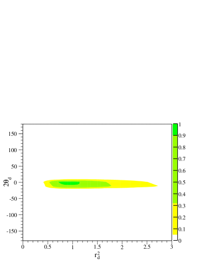
Figure 6: The allowed range for $r_{d}$ and $\theta_{d}$ after 2005.

Thus, in detail, the naive expectation mentioned above (based on comparing Figs 1(a) and 4(a)) is not borne out, i.e., surprisingly, NP $\sim 30-40\%$ of SM (with almost any phase) is still allowed! In view of above discussion, it is clear that such a large size of NP being allowed is due to the (as yet) sizable errors in the new data. The fact that any phase being allowed for such a sizable NP contribution is due to theory errors in data before summer, i.e., $\Delta m_{d}$ and $V_{ub}$ (since, just as before, in the absence of these errors, $\sigma_{d}$ is fixed for given $h_{d}$).

At this point, it is worth comparing the two parameterizations for NP: the $\left(r_{d}^{2},2\theta_{d}\right)$ plot in Fig 6 shows that $|2\theta_{d}|\lesssim 20^{\circ}$. However, this does not directly imply that NP phase ($\sigma_{d}$) is small since $2\theta_{d}$ is combination of $h_{d}$ and $\sigma_{d}$ (in particular, it is clear that for small $h_{d}$ large $\sigma_{d}$ still gives small $2\theta_{d}$). In this sense, $\left(h_{d},\sigma_{d}\right)$ is a more transparent parametrization of NP than $\left(r_{d}^{2},2\theta_{d}\right)$.

Note that $h_{d}$ up to $1.5$ is allowed, but only for $\sigma_{d}\sim 0$ since such NP only affects $\Delta m_{d}$ which has large theory errors. However, this implies aligning of NP phase with SM and hence a fine-tuning.

Clearly, unlike before summer, smaller experimental error (in $4^{th}$ data) will restrict the allowed $h_{d}$ (with arbitrary $\sigma_{d}$) to be less than $\sim 30\%$ and thus will sharpen the fine-tuning problem for models where the generic expectation is NP $\sim$ SM. Also, even if error in $4^{th}$ data is not improved, reducing theory errors in data before summer ($\Delta m_{d}$ and $V_{ub}$) is welcome since it will restrict the range of $\sigma_{d}$ allowed for, say, $h_{d}\sim 30\%$ (in addition to ruling out $h_{d}\sim 1$ (with $\sigma_{d}\sim 0$)). Thus, the allowed $h_{d}$ (with arbitrary $\sigma_{d}$) will be smaller, again leading to fine-tuning problem for NP models or in other words push $\Lambda_{\rm NMFV}$ to a higher scale.

There is another potential fine-tuning problem related to the Kaon system. There is no new data in $K$-system, but $\rho$, $\eta$ and hence SM contribution to $\varepsilon_{K}$ (even in presence of NP) is now known and accounts for observed $\varepsilon_{K}$. This implies that $h_{K}$ cannot be large: again, the naive expectation is that $h_{K}\ll 1$. Let us discuss the constraint from $\varepsilon_{K}$ quantitatively. In order to find the allowed region for $h_{K}$ after the 2004 summer results we use the relation (8) and scan over values of $h_{K}$ and $\sigma_{K}$ so that the resulting value is still within the combined constraints in yellow shown in fig. 4(a) The resulting range is given by

$$h_{K}=0-0.6\,\ \ \ \sigma_{K}=0-\pi\,,$$ (18)

although (as was the case before summer of 2004) even for $h_{K}\sim 1$ a large range of $\sigma_{K}$ (roughly half the physical range) is allowed (unlike for $h_{d}$, $\sigma_{d}$). This is demonstrated in fig. 5(b) which shows a plot of the region allowed by the combined recent measurements.

The fact that the $2\sigma$ excluded region has not changed too much before and after the summer can be easily understood from eq. 8. For $\sigma_{K}\sim 0$, as explained before, the $\eta$-intercept decreases (approaches zero) with increasing $h_{K}$ so that the hyperbola does not intersect the $V_{ub}$ circle in the allowed SM region at $1\sigma$, although, due to large theory errors, there is still an overlap with SM region with a lower CL ($2\sigma$). This explains the difference between Figs. 2(b) and 5(b) for $\sigma_{K}\sim 0$. Consider next $\sigma_{K}\sim\pi/2$. For $h_{K}\gtrsim 1$, the $\eta$-intercept is negative so that there is never an overlap with allowed (SM) region of $V_{ub}$ circle. Thus, $\sigma_{K}\sim\pi/2$ is excluded not only for $h_{K}\sim 1$ (for which the hyperbola does not intersect the $V_{ub}$ circle at all), but also for larger $h_{K}$ (cf. before summer 2004 where $h_{K}>1$ was allowed).

Thus, just as for $h_{d}$, the naive expectation for $h_{K}$ is not realized. In fact, $h_{K}\sim 0.6$ is still allowed – this is due to large theory errors in hadronic matrix elements. Thus it implies that only a mild increase in the scale $\Lambda_{\rm NMFV}$ or a mild suppression in the mixing angles (relative to the CKM angles) is required to fit the data.

Also, we checked that the correlation between $\left(h_{d},\sigma_{d}\right)$ and $\left(h_{K},\sigma_{K}\right)$ is weak at present due to the large errors.

During the last year no significant improvement in measurement related to the $B_{s}-\bar{B}_{s}$ system were obtained (and the SM contribution is independent of $\rho$, $\eta$ so that their direct measurement last year does not affect this analysis) . Consequently the constraint on $h_{s}-\sigma_{s}$ is unmodified and is described by fig. 3(a)

$$h_{s}=0-\infty\,.$$ (19)

The same figure shows also how the constraints on $h_{s}$ and $\sigma_{s}$ will change when $\Delta m_{S}$ will be measured. The particular plot in fig. 3(b) is for $\Delta m_{s}=(18.3\pm 0.3)ps^{-1}$.

We conclude this part with the following statement: even though the data significantly improved in the last two years (in the sense that new observables were measured), NP in $\Delta F=2$ amplitudes can still fit the data with arbitrary phases and size comparable to the SM contributions. This implies that only recently we have started to constrain NMFV models with $\Lambda_{\rm NMFV}=2-3\,$TeV.

IV $\Delta F=1$ transitions

So far in the above we discussed how NP is constrained using data only from $\Delta F=2$ processes. However, as demonstrated in Eq. (4) NP contributes not only to $\Delta F=2$ processes but also mediates $\Delta F=1$ transitions like $b\to s$ or $s\to d$. We shall analyze the implications of this scenario in the context of recent measurements of the CP asymmetries in $K\to\pi\bar{\nu}\nu$ (currently only an upper bound), $B\to\phi K_{S},\eta^{\prime}K_{S}$ and also $B\to K\pi$. As we will see, when dealing with the latter, two main difficulties are found: (i) due to the presence of strong phases, a computation of the hadronic matrix elements is required, which suffers from theoretical uncertainties. In order to get an estimate of the size of the uncertainties involved we shall obtain our results using two different hadronic models. For the $B\to K\pi$ transitions we shall use QCD factorization BBNS ; Beneke:2003zv ; BPRS and an SU(3) analysis (demonstrated here in complete form for the first time) whereas for $B\to\phi,\eta^{\prime}K$ case we shall use naive and QCD factorization. (ii) We shall see that, generically, in the presence of strong phases the number of unknown UV parameters is too large and therefore does not allow us to obtain bounds on the weak phases. Thus we are forced to make more assumptions which hold in a narrower class of NMFV models.

IV.1 Model dependence of the $\Delta F=1$ processes

We shall try to analyze our framework in as model-independent fashion as possible. However, a completely model independent analysis will be proven to be a non-trivial task given our present experimental and theoretical knowledge. Let us focus on the effective theory below the EWSB scale (or $M_{W}$) that is obtained in our framework, in particular in the context of $\Delta F=1$ processes. As we pointed out before, these have a much richer structure than the $\Delta F=2$ ones and in order to be able to obtain nontrivial results we therefore must restrict the definition of our framework. Let us now discuss in more detail the set of assumptions that define it. We consider these to be well motivated – for example, we will show in the next section that these assumptions hold in RS1 and various $Z^{\prime}$ models and therefore provides us with a way to test this framework. In addition we shall discuss how one can use our results to constraint other subclasses of the NMFV framework.

• NP induce only LH flavor-changing operators. This implies that our effective theory contains only operators which already exist in the SM one i.e. $O_{1-10}$ (see e.g. BBL for definition of the standard operator basis).

• The operators in the effective theory are obtained from integrating out color singlet particles (see e.g. Zp and references therein for related discussions).

As already discussed in section II the first assumption implies that there is a correlation between the observables related to $\Delta F=2$ and $\Delta F=1$ transitions. Note that this also clearly implies that the $\Delta F=1$ processes are governed by a single weak phase per transition. Furthermore the assumption (ii) implies that at the EWSB scale only the odd operators (since the color indices are trivially contracted), $O_{3,5,7,9}$, are being induced in the effective weak Hamiltonian. Consequently the amplitude for each transition is characterized by five UV parameters per transition, i.e. $C_{3,5,7,9}^{K,d,s}$ and a weak phase, $\sigma_{K,d,s}$. However, as we show next, even this reduction in the number of UV parameters is not enough to enable us to obtain a non-trivial constraint.

For the $s\to d$ transition processes, the only ones which are theoretically clean are the neutral and charge $K\to\pi\nu\bar{\nu}$ decays, which are related by isospin GNR . Thus we basically have only a single measurement with too large an uncertainty at this stage. The $b\to d$ case would seem to be better, since the B factories has provide us with more precise data on $B\to\rho\rho,\rho\pi,\pi\pi$. Extracting the UV parameters from the data in a theoretically clean way requires $SU(2)$ isospin analysis. However, since the above processes are dominated by SM tree level amplitudes, the resulting constraints on the above parameters are still rather weak at present. The $b\to s$ case is indeed better: there is data on the CP asymmetries in $B\to\phi,\eta^{\prime}K_{S}$ decays. Furthermore, the data on various $B\to K\pi$ processes has reached a precision level. And, more importantly (unlike the former cases), these decays are penguin dominated. Thus, with some limited theoretical input and the use of $SU(2)$ isospin, these decays can provide non-trivial constraints on our UV parameters. Below we show that without using a specific hadronic model for the matrix elements, the data from $S_{\eta^{\prime},\phi K_{S}}$ and the $B\to K\pi$ system provides us with three non-trivial data point. Using a specific hadronic model (like Naive factorization or QCD factorization) increases the number of data points at our disposal, but introduces additional theoretical uncertainties. This is still not enough in order to constrain five fundamental parameters, i.e., $C_{3,5,7,9}$ and the weak phase $\sigma_{s}$. The best we can do at this stage is to constrain frameworks with only two NP Wilson coefficients and a single weak phase. However, instead of considering this most general possibility, we take another route below, adding the following assumption.

• We choose a framework where NP affects only a single free NP Wilson coefficient (which is a linear combination of $C_{3,5,7,9}^{s}$ discussed above), which we find well motivated. Specifically, we consider the class of models in which the NP $\Delta F=1$ operators are aligned with the SM Z penguins.

This covers various $Z^{\prime}$ models (see Zprecent for recent related discussions), various little Higgs models and the RS1 framework. Note that, given (iii), the fact that we have more observables than input parameters implies that we can see whether these models are consistent with the present data and if they pass their first non-trivial test. The values of $C_{3,5,7,9}^{s}$ discussed above (at the $M_{W}$ scale) are

$$C_{3,5,7,9}^{s}(m_{W})\equiv C_{3,5,7,9}^{Z}(m_{W})h_{s}^{1}e^{i\sigma_{s}}$$ (20)

in such a way that when $h_{s}^{1}=1$ and $\sigma_{s}=0$ they coincide with the SM Z-penguin contribution.

We are led thus to consider the following extension of the weak $\Delta B=1$ Hamiltonian, including terms introduced by NP:

$${\cal H}_{W}^{SM}=\lambda_{u}^{(f)}[C_{1}O_{1}^{u}+C_{2}O_{2}^{u}]+\lambda_{c}^{(f)}[C_{1}O_{1}^{c}+C_{2}O_{2}^{c}]-\lambda_{t}^{(f)}\sum_{i=3}^{10}[C_{i}^{SM}(\mu)+h_{s}^{1}e^{i\sigma_{s}}C_{i}^{(Z)}(\mu)]O_{i}$$

with $f=d,s$. The operators $O_{i}$ are defined as in Ref. BBL and include the tree operators $O_{1,2}^{u,c}$, the QCD penguin operators $O_{3-6}$, and the electroweak penguin operators $O_{7-10}$.

The Wilson coefficients $C^{SM}_{3-10}(\mu)$ and $C^{(Z)}_{3-10}(\mu)$ are found using the standard method. First, one integrates out the $W$ and top quark at the $\mu=M_{W}$ scale, followed by running down to $\mu\sim m_{b}$. At the matching scale, the Wilson coefficients have an expansion in $\alpha_{s}(M_{W})$ of the form

$$\vec{C}(M_{W})\equiv\vec{C}^{SM}+\vec{C}^{(Z)} = \vec{C}_{s}^{(0)}(M_{W})+\frac{\alpha_{s}(M_{W})}{4\pi}\vec{C}_{s}^{(1)}(M_{W})+\frac{\alpha_{em}}{4\pi}[\vec{C}_{\rm ew}^{\gamma+b}(M_{W})$$ (22)

$$+\left(1+h_{s}^{1}e^{i\sigma_{s}}\right)\vec{C}_{\rm ew}^{Z}(M_{W})]\,.$$

In the matching condition we distinguish between the contributions from the photon penguin and box graphs $C^{\gamma+b}$ and from the $Z$ penguins $C^{Z}$. The Wilson coefficients at a low scale $\mu\sim m_{b}$ are obtained by running down with the $10\times 10$ anomalous dimension matrix of the operators $O_{1-10}$.

We quote below the values of the Wilson coefficients in Eq. (IV.1) at a low scale $\mu=4.25$ GeV. We used the following parameters in obtaining these results $\Lambda=225$ MeV, $m_{t}=170$ GeV, $\sin^{2}\theta_{W}=0.231$.

$$\begin{array}[]{c|cc|cccc|cccc}&C_{1}&C_{2}&C_{3}&C_{4}&C_{5}&C_{6}&C_{7}&C_{8}&C_{9}&C_{10}\\ \hline\cr\vec{C}^{(SM)}&1.086&-0.192&0.014&-0.036&0.01&-0.043&-0.0005&0.0004&-0.009&0.0017\\ \hline\cr 10^{3}\times\vec{C}^{(Z)}&0&0&1.80&-0.64&0.050&-0.298&1.182&0.446&-4.539&1.040\\ \hline\cr\end{array}$$ (26)

In the evaluation of the electroweak penguin coefficients we used the electromagnetic coupling $\alpha=1/129$.

A similar approach has been followed in section I to include the NP effects in the $\Delta S=2$, $\Delta B=2$ effective Hamiltonian. The weak phase appearing there, $2\sigma_{s}$, is related to the one in the $\Delta S=\Delta B=1$ effective Hamiltonian ($\sigma_{s}$). However, the magnitude of the NP in mixing will be in general different $h_{s}\neq h_{s}^{1}$.

IV.2 Analysis of $\Delta F=1$ transitions in $K$ system

We first briefly discuss the $K\to\pi\nu\bar{\nu}$ decay process which involves the $s\to d$ transition. In our framework the NP contributions are governed by $\sigma_{K}$, i.e., the same phase which controls the NP in $\varepsilon_{K}\,.$ The measurement of the charged mode has large errors so that the resulting constraint on $\sigma_{K}$ is rather weak. For the neutral mode $K_{L}\to\pi\nu\bar{\nu}$ there is presently only an upper bound so that the resulting constraint is much weaker. However, we still show the relation between these BR’s and the NP model parameters for future reference since the situation can dramatically change once more data is collected. For the charged mode we can relate the branching ratio to our NP parameters as follows

$${\rm BR}(K^{+}\to\pi^{+}\nu\bar{\nu})/\kappa_{+}\propto\left\{X^{2}\left(\eta^{2}+(\rho-1)^{2}\right)\left((h_{k}^{1})^{2}+2\cos\left(\sigma_{K}\right)h_{k}^{1}+1\right)A^{4}+\right.$$

$$\left.2X\left(\eta h_{k}^{1}\sin\left(\sigma_{K}\right)-(\rho-1)\left(h_{k}^{1}\cos\left(\sigma_{K}\right)+1\right)\right)P_{0}A^{2}+P_{0}^{2}\right\}\,,$$ (28)

(see e.g. kpn and refs. therein) where $X\sim 1.5$ and $P_{0}\sim 0.4$ BBL . A similar relation is obtained for the neutral decay mode. In the future, measuring the above processes will directly constrain $\sigma_{K}$, allowing for a comparison with the $\varepsilon_{K}$ result.

We now move to discuss in more details the constraints related to $b\to s$ transitions.

IV.3 $B\to\phi K_{S},\eta^{\prime}K_{S}$ transitions

An important source of information about the new physics in $b\to s$ transitions comes from time-dependent CP violation in $B$ decays into CP eigenstates. The relevant parameters for the $B^{0}(t)\to f$ transition are defined in terms of the ratio of amplitudes

$$\lambda_{f}=e^{-i\phi_{M}}\frac{\bar{A}_{f}}{A_{f}}$$ (29)

where $\phi_{M}$ is the $B^{0}-\bar{B}^{0}$ mixing phase, and $A_{f},\bar{A}_{f}$ are the $B^{0}\to f$ and $\bar{B}^{0}\to f$ decay amplitudes, respectively. The time-dependent CP asymmetry parameters $S_{f}$ and $C_{f}$ are given in terms of these parameters by

$$S_{f}=\frac{2\mbox{Im }\lambda_{f}}{1+|\lambda_{f}|^{2}}\,,\qquad C_{f}=\frac{1-|\lambda_{f}|^{2}}{1+|\lambda_{f}|^{2}}$$ (30)

Assuming that the amplitudes $A_{f},\bar{A}_{f}$ are dominated by one single weak phase, the $S_{f}$ parameter gives a direct measurement of the interference of this phase with the $B^{0}-\bar{B}^{0}$ mixing amplitude. One such case is the tree mediated decay $B\to\psi K_{S}$, which measures the $B^{0}-\bar{B}^{0}$ mixing phase. Allowing for NP in the $B^{0}-\bar{B}^{0}$ mixing amplitude, this relation is modified in our framework as mentioned in Sec. III

$$S_{\psi K_{S}}=\sin(2\beta+2\theta_{d})$$ (31)

with $1+h_{d}e^{i\sigma_{d}}=r_{d}^{2}e^{2i\theta_{d}}$. The experimental result for $S_{\psi K_{S}}$ is shown in Table 1.

Next we consider the penguin-mediated decays $b\to s\bar{q}q$, which have in general a more complicated structure. Allowing for NP as described by the effective Hamiltonian Eq. (IV.1), the general form of the decay amplitude can be written as

$$A_{f}=\lambda_{c}^{(s)}P_{f}(1+e^{i\gamma}d_{f}e^{i\theta_{f}}+h_{s}^{1}e^{-i\sigma_{s}}q_{f}^{c}e^{i\phi_{f}^{c}}(1+R_{b}\lambda^{2}e^{i\gamma}))$$ (32)

where $R_{b}=\sqrt{{\bar{\rho}}^{2}+{\bar{\eta}}^{2}}$. The different terms in this formula arise from the operators in the weak Hamiltonian Eq. (IV.1) as follows: $P_{f}$ is contributed by the matrix elements of $O_{1,2}^{c}$ and $O_{3-10}$ with the SM Wilson coefficients; the $d_{f}e^{i\theta_{f}}$ arises from the operators $O_{1,2}^{u}$; finally, the terms proportional to $q_{f}e^{i\phi_{f}^{c}}$ are contributed by the operators $O_{3-10}$ with the Wilson coefficients $C_{i}^{Z}(\mu)$. The small correction $\sim\lambda^{2}R_{b}\sim O(1\%)$ is introduced by the fact that NP appears in Eq. (IV.1) multiplying the CKM coefficient $\lambda_{t}^{(s)}$.

In the absence of the $d_{f}$ term (usually called the ‘SM contamination’), and assuming the validity of the SM, the amplitude Eq. (32) gives a CP asymmetry parameter $S_{f}=-\eta_{CP}\sin(2\beta+2\theta_{d})$, where $\eta_{CP}$ is the CP eigenstate of the final state. In particular, $S_{f}$ measured in these decays must be directly related to the corresponding parameter in $B\to\psi K_{S}$. Any significant deviation from zero of the difference $-\eta_{CP}S_{f}-S_{\psi K_{S}}$ can be therefore interpreted as new physics London:1997zk ; Grossman:1996ke .

We show in Table 2 the current measured values of the CP violating parameters $S_{f}$ and $C_{f}$ for several decays mediated by the $b\to s$ penguin. The individual results for $S_{f}$ from BABAR and BELLE are listed, together with their world average. For reference, we give also the corresponding result for $B\to J/\psi K_{S}$, to which they are equal in the SM in the limit of the decay amplitude being dominated by the penguin. The results display a deviation from the naive SM expectation $-\eta_{CP}S_{f}=S_{\psi K_{S}}$ of roughly $2\sigma$. The agreement improved after the most recent results reported at the Lepton-Photon 2005 conference LP05 .

A nonzero difference $-\eta_{CP}S_{f}-S_{\psi K_{S}}$ can be introduced from terms in the decay amplitude with a weak phase different from that of the penguin. Such terms are present in the SM, where they originate from the matrix elements of $O_{1,2}^{u}$, which are multiplied with the CKM coefficient $\lambda_{u}^{(s)}=e^{-i\gamma}|\lambda_{u}^{(s)}|$ (parameterized by $\sim d_{f}e^{i\phi_{f}}$ in Eq. (32)). Since such contributions are CKM- and loop-suppressed, they are expected to be small.

The SM contamination in the differences $\Delta_{f}=-\eta_{CP}S_{f}-S_{\psi K_{S}}$ has been studied using several methods. In Refs. Grossman:2003qp ; Gronau:2003kx , these effects have been bound using SU(3) flavor symmetry, and inputs from the measured branching fractions of $b\to d$ modes. This method allows also the study of correlations with data on $C_{f}$ and has been recently extended also to 3-body modes 3body . Further applications of these bounds, with additional dynamical input, have been presented in Ref. boundsplus .

A different approach makes use of QCD factorization in the heavy quark limit, to compute the matrix elements of the operators in the weak Hamiltonian. Such computations were performed in Beneke:2003zv ; Beneke:2005pu and found to give small positive results for the differences $-\eta_{CP}S_{f}-S_{\psi K_{S}}$ (see Ref. Beneke:2005pu for a recent update). On the other hand, the observed sign of this difference in the experimental data is predominantly negative, although with significant errors. Therefore it is natural to attempt an explanation of the data in terms of new physics contributions to the weak effective Hamiltonian.

$f$	$-\eta_{CP}S_{f}$			$C_{f}$
	BABAR	BELLE	WA	WA
$\phi K_{S}$	$0.50\pm 0.25^{+0.07}_{-0.04}$	$0.44\pm 0.27\pm 0.05$	$0.47\pm 0.19$	$-0.09\pm 0.14$
$\eta^{\prime}K_{S}$	$0.36\pm 0.13\pm 0.03$	$0.62\pm 0.12\pm 0.04$	$0.50\pm 0.09$	$-0.07\pm 0.07$
$\pi^{0}K_{S}$	$0.35^{+0.30}_{-0.33}\pm 0.04$	$0.22\pm 0.47\pm 0.08$	$0.31\pm 0.26$	$-0.02\pm 0.13$
$J/\psi K_{S}$			$0.687\pm 0.032$

Table 2: Experimental results BaBe for the CP asymmetry parameters in neutral $B$ decay into CP eigenstates mediated by the $b\to s\bar{q}q$ transition. For reference we show also the corresponding parameter measured in $B\to\psi K_{S}$ decays.

In the remainder of this section, we will study the implications of these data for the NP framework considered here, in particular the constraints on the parameters $(h_{s}^{1},\sigma_{s})$. Some aspects of our analysis have been partially considered in previous work, so a brief review is in order.

An important question concerns the assumptions built into the NMFV, in particular assumption (i) of the NP inducing only LH flavor-changing operators. Due to the different parity of the final state in $S_{\phi K},S_{\eta^{\prime}K}$ the resulting asymmetries are sensitive to the chiral structure of the NP contributions Kagan . In Endo:2004dc , Endo, Mishima, and Yamaguchi demonstrated that a possible difference between the mixing-induced CP-asymmetries in $B\to\phi K_{S}$ and $B\to\eta^{\prime}K_{S}$ can be easily explained by NP-induced operators with LH chiralities for a wide range of weak phases and amplitudes. This observation validates the assumption (i) of the NMFV approach (see Sec. IV.A).

Another important information yielded by the recent measurements is that, with left handed NP operators LMP , the data can be accounted even if the NP contributions are subdominant. Thus it is interesting to examine whether the data can be explained by $O(1)$ modification of the SM electroweak operators (as in our framework). Such a scenario occurs in many models with NP mediated by a $Z^{\prime}$ gauge boson Zp . Our main motivation however to discuss this is that it was recently shown (before the summer results) in APS that this is exactly the case in RS1 models with low KK masses and bulk custodial isospin.

We describe next the details of our analysis. We add new terms $q_{f}e^{i\phi_{f}}$ in the $b\to s$ amplitude in Eq. (32) induced by the NP terms in the weak effective Hamiltonian (IV.1). The coefficient $q_{f}e^{i\phi_{f}}$ is related to matrix elements of the operators $O_{3-10}$ with appropriate Wilson coefficients $C_{i}^{Z}$. We computed these matrix elements for several final states $f$ of interest using: a) naive factorization Naive and b) the QCD factorization relations using the heavy quark limit BBNS , including the leading radiative corrections and chirally enhanced terms. The results of this analysis are shown in the plots of Fig. 7, where the left column is for the naive factorization case and the right one is for the QCD factorization case. In the numerical evaluation of the factorization formulas we used the hadronic parameters quoted in Ref. Beneke:2003zv with the exception of the quark masses, for which we take $m_{b}(m_{b})=4.8\pm 0.1$ GeV and $m_{s}(2\,GeV)=0.11\pm 0.025$ GeV.

This type of analysis overlaps partially with previous work done in Ref. BFRS , where constraints on several NP scenarios were obtained from mixing-induced CP violation in $b\to s$ decays. The parameters $\varepsilon_{z}e^{i\theta_{z}}$ introduced in BFRS describing NP induced through Z$-$penguins are similar to the parameters $(h_{s}^{1},\sigma_{s})$ used here. Ref. BFRS used leading order factorization to compute the matrix elements of the relevant weak Hamiltonian operators. There are important differences between our analysis and that presented in Ref. BFRS , which we discuss next. First, we take into account also the NP present in $B^{0}-\bar{B}^{0}$ mixing, parameterized by the $(h_{d},\sigma_{d})$. This is done by performing a correlated analysis of these two types of processes. Second, the analysis of BFRS does not take into account experimental information on direct CP asymmetries. The reason for this is that at leading order in QCD factorization, the strong phases vanish. This implies that the direct CP asymmetries are predicted to vanish, and thus no information is gained at this order. In our fits the $A_{CP}$ data is included as inputs for the QCD factorization case.

$\begin{array}[]{c@{\hspace{0.2in}}c}\includegraphics[width=216.81pt]{sphik_nv}\hfil\hskip 14.45377pt&\includegraphics[width=216.81pt]{sphik_bbns}\\ \mbox{\bf(a)}\hfil\hskip 14.45377pt&\mbox{\bf(b)}\\ \includegraphics[width=216.81pt]{setapk_nv}\hfil\hskip 14.45377pt&\includegraphics[width=216.81pt]{setapk_bbns}\\ \mbox{\bf(c)}\hfil\hskip 14.45377pt&\mbox{\bf(d)}\\ \includegraphics[width=216.81pt]{setapksphik_nv}\hfil\hskip 14.45377pt&\includegraphics[width=216.81pt]{setapksphik_bbns}\\ \mbox{\bf(e)}\hfil\hskip 14.45377pt&\mbox{\bf(f)}\end{array}$

Figure 7: The constraints on $h_{s}^{1}$ and $\sigma_{s}$ from various $\Delta F=1$ processes. Left column: naive factorization results. Right column: QCD factorization results. The various rows are respectively for (from top to bottom): $B\rightarrow\phi K_{S}$, $B\rightarrow\eta^{\prime}K_{S}$, the two combined.

IV.4 $B\to K\pi$ transitions

The $B\to K\pi$ decays are penguin-dominated processes, with subleading contributions coming from tree and electroweak penguin amplitudes. In this respect they are similar to the $B\to\phi K_{S}$ and $\eta^{\prime}K_{S}$ decays considered previously, however with a larger “up-type” contamination.

In the previous subsection we showed that the time-dependent CP asymmetry parameter $S_{f}$ in $B^{0}(t)\to f$ can be used to constrain the NP parameters $(h_{s}^{1},\sigma_{s})$, provided that the hadronic parameters determining the NP contribution are known. Writing the amplitude for a generic $B\to f$ mode as

$$A(\bar{B}^{0}\to f)=P_{f}(1+d_{f}e^{i\psi_{f}}e^{-i\gamma}+h_{s}^{1}e^{i\sigma_{s}}q_{f}e^{i\phi_{f}})\,,$$ (33)

the NP parameters $(h_{s}^{1},\sigma_{s})$ have been constrained using dynamical computations of the hadronic parameters $(d,\psi)$ and $(q,\phi)$.

In this subsection we show that in the particular case of the $B^{0}\to K_{S}\pi^{0}$ decay, these parameters can be determined from data on other $B\to K\pi$ decays, using only flavor SU(3) symmetry and minimal assumptions about the smallness of certain contributions. Some of these assumptions are satisfied at leading order of the heavy mass expansion in $\Lambda/m_{b}$, and are explicitly checked in dynamical computations of the nonleptonic decay amplitudes in factorization BBNS ; Beneke:2003zv ; BPRS . We estimate the corrections introduced by the remaining assumptions by comparing with the results of such dynamical computations. In principle, the output of such an analysis allows also a direct test of the QCD factorization computation of these hadronic parameters. The current precision of the data is however not sufficient for performing a significant test. Tests for NP in these modes using related methods were also presented in Refs. xx ; xx1 ; xx2 ; xx3 ; xx4 .

We give also the results for the constraints on $(h_{s}^{1},\sigma_{s})$ using as input the QCD factorization results for the hadronic parameters $(d,\psi)$ and $(q,\phi)$ in Eq. (33).

Before proceeding with the details of our analysis we list our data points. Altogether we have 9 (10 when we include the constraint on the CKM phase as we shall do eventually using the results of our $\Delta F=2$ analysis) data points. These are given by four branching ratios $B^{-,0}\to\pi^{-}\bar{K}^{0},\pi^{0}\bar{K}^{-},\pi^{+}K^{-},\pi^{0}K^{0}\,$, four direct CP asymmetries and a single time-dependent CP asymmetry $S_{K_{S}\pi^{0}}$. The corresponding experimental values are listed in Table 3.

We start by neglecting the NP and discuss the most general form for these decay amplitudes in the SM. The structure of the $B\to K\pi$ decay amplitudes, assuming only isospin symmetry, can be written in terms of graphical amplitudes as (see, e.g. GHLR )

$$A(B^{-}\to\pi^{-}\bar{K}^{0})=\lambda_{u}^{(s)}(P_{uc}+A)+\lambda_{t}^{(s)}(P_{tc}+EW_{P}+\frac{1}{2}EW_{C}-EW_{E})$$ (34)

$$\sqrt{2}A(B^{-}\to\pi^{0}K^{-})=\lambda_{u}^{(s)}(-P_{uc}-A-T-C)+\lambda_{t}^{(s)}(-P_{tc}-EW_{P}+EW_{T}+EW_{C}+EW_{E})$$

$$A(\bar{B}^{0}\to\pi^{+}K^{-})=\lambda_{u}^{(s)}(-P_{uc}-T)+\lambda_{t}^{(s)}(-P_{tc}-EW_{P}+EW_{C}-\frac{1}{2}EW_{E})$$

$$\sqrt{2}A(\bar{B}^{0}\to\pi^{0}\bar{K}^{0})=\lambda_{u}^{(s)}(P_{uc}-C)+\lambda_{t}^{(s)}(P_{tc}+EW_{P}+EW_{T}+\frac{1}{2}EW_{C}+\frac{1}{2}EW_{E})$$

The notation adopted implies the use of the unitarity of the CKM matrix to eliminate the $c$-quark CKM factor as $\lambda_{c}^{(s)}=-\lambda_{u}^{(s)}-\lambda_{t}^{(s)}$. We combined the QCD penguin amplitudes as $P_{ut}=P_{u}-P_{t}$ and $P_{ct}=P_{c}-P_{t}$.

The graphical amplitudes appearing in Eqs. (34) arise as matrix elements of specific operators in the weak Hamiltonian, as follows: the operators $O_{1,2}^{u,c}$ give rise to the tree $T$, color-suppressed $C$, weak annihilation $A$ and $u,c$-penguin $P_{u},P_{c}$ amplitudes. The matrix elements of the electroweak penguin operators $Q_{7-10}$ appear in several possible combinations: color-allowed $EW_{T}$, color-suppressed $EW_{C}$, penguin-type contractions $EW_{P}$ and weak annihilation $EW_{E}$.

In the presence of new physics as described by the weak Hamiltonian Eq. (IV.1), the QCD and EW penguin amplitudes can be split into contributions which contain, respectively do not contain, the NP factor $h_{s}^{1}e^{i\sigma_{s}}$ as follows

$$P_{t}\to P_{t}+h_{s}^{1}e^{i\sigma_{s}}P_{Z}$$ (35)

$$EW_{i}\to EW_{i}+h_{s}^{1}e^{i\sigma_{s}}EW_{i}^{(Z)}$$ (36)

The new penguin amplitude $P_{Z}$ is proportional to the Wilson coefficients $C_{3-6}^{Z}$, and the new EWP amplitudes are proportional to the corresponding Wilson coefficients $C_{7-10}^{Z}$. In the remainder of this part we will assume the SM form of the $B\to K\pi$ amplitudes. Their modification to include NP effects using Eq. (35) is straightforward and will be included below.

Isospin symmetry gives one relation among these amplitudes

$$A(B^{-}\to\pi^{-}\bar{K}^{0})+\sqrt{2}A(B^{-}\to\pi^{0}K^{-})=A(\bar{B}^{0}\to\pi^{+}K^{-})+\sqrt{2}A(\bar{B}^{0}\to\pi^{0}\bar{K}^{0})\,.$$ (37)

Counting hadronic parameters gives 6 independent complex amplitudes (8 coefficients of the $\lambda_{u,t}$ CKM factors minus two relations from (37)). Taking into account that one unphysical phase can be eliminated, this gives 11 independent real hadronic parameters. Together with the CKM phase, this counting shows that the $K\pi$ system is parameterized by 12 unknown parameters, which can not be fixed with only the help of the 9 data points in Table 2 (even if the CKM phase is added as an input). In other words, the most general form Eq. (34) contains too many amplitudes to be predictive, and additional input is necessary. We will be very explicit about the assumptions made, and discuss possible tests for their validity.

Assumption A. In the heavy quark limit, weak annihilation diagrams are power suppressed by $\Lambda/m_{b}$ relative to the tree and penguin amplitudes BBNS ; Beneke:2003zv ; BPRS . This is a theoretically clean approximation, although the numerical size of the power corrections $O(\Lambda/m_{b})$ could be significant. In this limit we can neglect the weak annihilation amplitudes $A,EW_{E}$ appearing in Eqs. (34). This approximation by itself does not reduce the number of $K\pi$ independent amplitudes, but will be required in conjunction with the approximation B. introduced below.

Assumption B. Flavor SU(3) symmetry and the neglect of the matrix elements related to electroweak penguins $Q_{7,8}$. This approximation is justified in the SM because of the smallness of the Wilson coefficients $C_{7,8}$ relative to $C_{9,10}$ (see Eq. (26)). In the presence of new physics mediated by the $Z$ coupling (IV.1), this inequality still holds $C_{7,8}^{(Z)}<C_{9,10}^{(Z)}$, but the Wilson coefficients $C_{7,8}^{(Z)}$ are not negligible compared with the QCD penguin coefficients $C_{3-6}^{(Z)}$. Their effects must be therefore included in our analysis.

The latter assumption allows a reduction in the number of electroweak penguin amplitudes, and gives four relations for these amplitudes. These relations follow from SU(3) symmetry, and were derived in Refs. NeRo ; BuFl ; GPY . The first relation does not require the approximation A. and relates the combination $EW_{T}+\frac{3}{2}EW_{C}$ as NeRo

$$EW_{T}+\frac{3}{2}EW_{C}=\frac{3}{2}\kappa_{+}(T+C)$$ (38)

where $\kappa_{\pm}$ are given by ratios of Wilson coefficients of the dominant EW penguins $O_{9,10}$ as

$$\kappa_{\pm}\equiv\frac{C_{9}\pm C_{10}}{C_{1}\pm C_{2}}$$ (39)

Adopting also the approximation A., two additional identities can be written down, which fix all individual EW penguin amplitudes in terms of the $T,C$ and $P_{uc}$ amplitudes GPY . The first relation holds for any values of $\kappa_{\pm}$

$$EW_{C}=\frac{1}{2}\kappa_{+}(T+C)+\frac{1}{2}\kappa_{-}(C-T)\,.$$

and the second relation

$$EW_{P}=\kappa P_{u}\,.$$ (40)

assumes furthermore the equality $\kappa_{+}\simeq\kappa_{-}\equiv\kappa$, which holds to a good precision in the SM. It continues to hold in any new physics model for which $C_{10}(M_{W})$ is subdominant, including the class of models considered here.

The approximations A. and B. taken together reduce the number of individual hadronic parameters to 4 complex amplitudes: $P_{ut},P_{ct},T,C$ (minus an overall phase). Counting in also $\gamma$, this gives 8 unknown real parameters, which can be extracted from data. This is essentially the approach proposed in Ref. London for determining $\gamma$ from $B\to K\pi$ data alone.

Including also the NP effects through the substitutions Eq. (35) introduces several new parameters: $(h_{s}^{1},\sigma_{s})$ and the NP penguins $P_{Z}$ and $EW_{i}^{Z}$. This renders the system again undetermined. The $EW_{i}^{Z}$ amplitudes can be expressed in terms of the tree amplitudes, using relations similar to those for $EW_{i}$. The relation similar to Eq. (38) is

$$EW_{T}^{Z}+\frac{3}{2}EW_{C}^{Z}=\frac{3}{2}\kappa_{+}^{Z}(T+C)+\frac{3}{2}\Delta_{1}(T+C)$$ (41)

where $\kappa_{\pm}^{Z}$ are given by

$$\kappa_{\pm}^{Z}\equiv\frac{C_{9}^{Z}\pm C_{10}^{Z}}{C_{1}\pm C_{2}}$$ (42)

and $\Delta_{1}$ is a correction proportional to $C_{7,8}^{Z}$. Inspection of the Wilson coefficients in Eq. (26) shows that their effects can be significant, and have to be included. In QCD factorization this coefficient is given explicitly by

$$\Delta_{1}=\frac{r_{\chi}^{M}a_{8Z}^{c}-a_{7Z}^{c}}{a_{1}+a_{2}}=-\frac{C_{7}^{Z}+C_{8}^{Z}/N_{c}}{(C_{1}+C_{2})(1+1/N_{c})}+r_{\chi}^{K}\frac{C_{8}^{Z}+C_{7}^{Z}/N_{c}}{(C_{1}+C_{2})(1+1/N_{c})}+O(\alpha_{s})$$ (43)

where we used the notations of Beneke:2003zv for the coefficients $a_{i}$. A subscript $Z$ means that $a_{iZ}$ has to be computed using the $C_{i}^{Z}$ Wilson coefficients. We retained here also the $a_{8Z}^{c}$ term, although it is formally power suppressed by the factor $r_{\chi}^{K}=2M_{K}^{2}/(m_{b}(m_{q}+m_{s}))$. However, numerically it is comparable with the $a_{7Z}^{c}$ term, and it partially cancels it. Using the Wilson coefficients in Eq. (26), the effect of $\Delta_{1}$ is a 6% increase in the value of $\kappa_{+}$ (in absolute value). This shows that the contributions from $C_{7,8}^{Z}$ can be neglected to a very good approximation in the relation Eq. (41).

The relations analogous to Eqs. (IV.4), (40) read

$$EW_{C}^{Z}=\frac{1}{2}\kappa_{+}^{Z}(T+C)+\frac{1}{2}\kappa_{-}^{Z}(C-T)+\Delta_{2}(T+C)$$ (44)

$$EW_{P}^{Z}=\kappa^{Z}P_{u}+\Delta_{3}\,.$$ (45)

with $\kappa^{Z}\equiv\kappa_{+}^{Z}\sim\kappa_{-}^{Z}$, and the correction terms $\Delta_{2,3}$ contain again the contributions proportional to $C_{7,8}^{Z}$. We will need only $\Delta_{2}$, which is given in QCD factorization by BBNS ; Beneke:2003zv

$$\Delta_{2}=\frac{r_{\chi}^{K}a_{8Z}^{c}}{a_{1}+a_{2}}=r_{\chi}^{K}\frac{C_{8}^{Z}+C_{7}^{Z}/N_{c}}{(C_{1}+C_{2})(1+1/N_{c})}+O(\alpha_{s})$$ (46)

This gives that the $C_{7,8}^{Z}$ contributions to the relation Eq. (44) are both power suppressed and color suppressed. However, they appear multiplied with the chirally enhanced coefficient $r_{\chi}^{K}$, so for consistency with Eq. (41) we will include them in the following. Numerically the effect of $\Delta_{2}$ is a negative shift (again in absolute value) in $\kappa_{+}$ of $\sim-40\%$. However, when substituted in the $\bar{B}\to K\pi$ amplitudes, the overall contribution from $Q_{7,8}$ is negligible (below 1% of the total amplitude) over most of the parameter space. Therefore we will neglect these contributions in our fit.

Counting the number of parameters, we have now in addition to the 7 SM parameters, $P_{ut},P_{ct},T,C$, another 4 unknown parameters $h_{s}^{1},\sigma_{s},P_{Z}$. This renders the system undetermined. To be able to proceed, we make one last approximation.

Assumption C. Our final approximation here is to neglect the amplitude $P_{ut}$ which is doubly Cabibbo suppressed by the small CKM coefficient $\lambda_{u}^{(s)}$.

With this approximation, the $K\pi$ system is described in the presence of NP by 4 complex hadronic amplitudes $P_{ct},T,C,P_{Z}$ and the two NP parameters $(h_{s}^{1},\sigma_{s})$, altogether 9 unknowns (the CKM phase will be taken as an input from our $\Delta F=2$ analysis). The number of hadronic parameters can be reduced by one if we consider also the decay $B^{+}\to\pi^{0}\pi^{+}$. As this mode is dominated by a SM tree level transition, it receives a negligible NP contribution. Neglecting small electroweak penguin contributions, the amplitude for this decay is

$$\sqrt{2}A(B^{-}\to\pi^{0}\pi^{-})=\lambda_{u}^{(d)}(T+C)$$ (47)

with branching fraction BR$(B^{+}\to\pi^{0}\pi^{+})=(5.5\pm 0.6)\times 10^{-6}$ hfag . Using the branching fraction for this mode as an input eliminates the hadronic amplitude $|T+C|$, and reduces the number of unknown parameters to 8.

	$Br\,(\times 10^{-6})$	$A_{CP}$
$B^{-}\to\pi^{-}\bar{K}^{0}$	$24.1\pm 1.3$	$-0.02\pm 0.04$
$B^{-}\to\pi^{0}K^{-}$	$12.1\pm 0.8$	$0.04\pm 0.04$
$B^{0}\to\pi^{+}K^{-}$	$18.9\pm 0.7$	$-0.11\pm 0.02$
$B^{0}\to\pi^{0}\bar{K}^{0}$	$11.5\pm 1.0$	$0.01\pm 0.16$
$S_{K_{S}\pi^{0}}$	$0.34\pm 0.28$

Table 3: World averages of $B\to K\pi$ branching fractions, direct CP asymmetries and the $S_{K_{S}\pi^{0}}$ parameter hfag .

The most general parameterization of the $\bar{B}\to K\pi$ amplitudes compatible with the assumptions A.,B.,C. can be written as

$$A(B^{-}\to\pi^{-}\bar{K}^{0})=\lambda_{c}^{(s)}P_{ct}(1+\frac{1}{3}\delta_{EW}\varepsilon_{C}e^{i\phi_{C}}+h_{s}^{1}e^{i\sigma_{s}}[p_{Z}e^{i\phi_{Z}}+\frac{1}{3}\delta_{EW}^{Z}\varepsilon_{C}e^{i\phi_{C}}])$$ (48)

$$\sqrt{2}A(B^{-}\to\pi^{0}K^{-})=-\lambda_{c}^{(s)}P_{ct}(1-\delta_{EW}\varepsilon e^{i\phi}+\frac{1}{3}\delta_{EW}\varepsilon_{C}e^{i\phi_{C}}$$ (49)

$$\hskip 85.35826pt+h_{s}^{1}e^{i\sigma_{s}}[p_{Z}e^{i\phi_{Z}}-\delta_{EW}^{Z}\varepsilon e^{i\phi}+\frac{1}{3}\delta_{EW}^{Z}\varepsilon_{C}e^{i\phi_{C}}]+e^{-i\gamma}\varepsilon e^{i\phi})$$

$$A(\bar{B}^{0}\to\pi^{+}K^{-})=-\lambda_{c}^{(s)}P_{ct}(1-\frac{2}{3}\delta_{EW}\varepsilon_{C}e^{i\phi_{C}}+h_{s}^{1}e^{i\sigma_{s}}[p_{Z}e^{i\phi_{Z}}-\frac{2}{3}\delta^{Z}_{EW}\varepsilon_{C}e^{i\phi_{C}}]+e^{-i\gamma}\varepsilon_{T}e^{i\phi_{T}})$$

$$\sqrt{2}A(\bar{B}^{0}\to\pi^{0}\bar{K}^{0})=\lambda_{c}^{(s)}P_{ct}(1+\delta_{EW}\varepsilon_{T}e^{i\phi_{T}}+\frac{1}{3}\delta_{EW}\varepsilon_{C}e^{i\phi_{C}}$$ (50)

$$\hskip 85.35826pt+h_{s}^{1}e^{i\sigma_{s}}[p_{Z}e^{i\phi_{Z}}+\delta^{Z}_{EW}\varepsilon_{T}e^{i\phi_{T}}+\frac{1}{3}\delta^{Z}_{EW}\varepsilon_{C}e^{i\phi_{C}}]-e^{-i\gamma}\varepsilon_{C}e^{i\phi_{C}})$$

We introduced here the tree/penguin ratios $(\varepsilon_{i},\phi_{i})$, and the reduced NP penguin parameters $(p_{Z},\phi_{Z})$, defined as

$$\varepsilon_{T}e^{i\phi_{T}}=\frac{|\lambda_{u}^{(s)}|}{|\lambda_{c}^{(s)}|}\frac{T}{P_{ct}}\,,\quad\varepsilon_{C}e^{i\phi_{C}}=\frac{|\lambda_{u}^{(s)}|}{|\lambda_{c}^{(s)}|}\frac{C}{P_{ct}}\,,\quad\varepsilon e^{i\phi}=\frac{|\lambda_{u}^{(s)}|}{|\lambda_{c}^{(s)}|}\frac{T+C}{P_{ct}}\,,\quad p_{Z}e^{i\phi_{Z}}=\frac{P_{Z}}{P_{ct}}\,.$$ (51)

The parameters $\delta_{EW}$ and $\delta_{EW}^{Z}$ describe the contributions of the two types of electroweak penguin operators $C_{9,10}$ and $C_{9,10}^{Z}$, respectively. Their numerical values can be obtained from Eq. (26)

$$\delta_{EW}=-\frac{3}{2}\frac{|\lambda_{c}^{(s)}|}{|\lambda_{u}^{(s)}|}\frac{C_{9}+C_{10}}{C_{1}+C_{2}}\simeq 0.65\,,\qquad\delta_{EW}^{Z}=-\frac{3}{2}\frac{|\lambda_{c}^{(s)}|}{|\lambda_{u}^{(s)}|}\frac{C_{9}^{Z}+C_{10}^{Z}}{C_{1}+C_{2}}\simeq 0.287\,.$$ (52)

We will use as hadronic inputs the following ratios of CP-averaged branching fractions

$$R_{\pi}=\frac{2Br(B^{+}\to\pi^{0}\pi^{+})}{Br(B^{+}\to K^{0}\pi^{+})}=0.456\pm 0.055\,,\qquad R_{c}=\frac{2Br(B^{+}\to\pi^{0}K^{+})}{Br(B^{+}\to K^{0}\pi^{+})}=1.004\pm 0.086$$ (53)

$$R_{n}=\frac{Br(B^{0}\to K^{+}\pi^{-})}{Br(B^{+}\to K^{0}\pi^{+})}\frac{\tau_{B^{+}}}{\tau^{B^{0}}}=0.816\pm 0.057\,,\qquad R_{0}=\frac{2Br(B^{0}\to K_{S}\pi^{0})}{Br(B^{+}\to K^{0}\pi^{+})}\frac{\tau_{B^{+}}}{\tau^{B^{0}}}=1.032\pm 0.106$$

together with the direct CP asymmetries and the $S_{K_{S}\pi^{0}}$ parameter in Table 2. We will use the weak phase $\gamma$ as determined from the global CKM fit  CKMfitter

$$\gamma=(57^{+13}_{-8})^{\circ}$$ (55)

This gives a total of 9 data points which can be used to constrain the 8 hadronic parameters $(\varepsilon,\phi),(\varepsilon_{C},\phi_{C}),(p_{Z},\phi_{Z})$ and the NP parameters $(h_{s}^{1},\sigma_{s})$ from data.

For the purposes of a numerical analysis, it is convenient to simplify the theoretical expressions for the decay amplitudes, by introducing a new penguin amplitude

$$P\equiv\lambda_{c}^{(s)}P_{ct}(1+\frac{1}{3}\delta_{EW}\varepsilon_{C}e^{i\phi_{C}})$$ (56)

and redefining the ratios of amplitudes as

$$\frac{\varepsilon_{i}e^{i\phi_{i}}}{1+\frac{1}{3}\delta_{EW}\varepsilon_{C}e^{i\phi_{C}}}\to\varepsilon_{i}e^{i\phi_{i}}\,,\qquad i=T,C$$ (57)

$$\frac{p_{Z}e^{i\phi_{Z}}+\frac{1}{3}\delta_{EW}^{Z}\varepsilon_{C}e^{i\phi_{C}}}{1+\frac{1}{3}\delta_{EW}\varepsilon_{C}e^{i\phi_{C}}}\to p_{Z}e^{i\phi_{Z}}\,.$$ (58)

Expressed in terms of the redefined parameters, the $B\to K\pi$ amplitudes in Eqs. (48) are given by

$$A(B^{-}\to\pi^{-}\bar{K}^{0})=P(1+h_{s}^{1}e^{i\sigma_{s}}p_{Z}e^{i\phi_{Z}})$$ (59)

$$\sqrt{2}A(B^{-}\to\pi^{0}K^{-})=-P(1-\delta_{EW}\varepsilon e^{i\phi}+e^{-i\gamma}\varepsilon e^{i\phi}+h_{s}^{1}e^{i\sigma_{s}}[p_{Z}e^{i\phi_{Z}}-\delta_{EW}^{Z}\varepsilon e^{i\phi}])$$ (60)

$$A(\bar{B}^{0}\to\pi^{+}K^{-})=-P(1-\delta_{EW}\varepsilon_{C}e^{i\phi_{C}}+e^{-i\gamma}\varepsilon_{T}e^{i\phi_{T}}+h_{s}^{1}e^{i\sigma_{s}}[p_{Z}e^{i\phi_{Z}}-\delta^{Z}_{EW}\varepsilon_{C}e^{i\phi_{C}}])$$

$$\sqrt{2}A(\bar{B}^{0}\to\pi^{0}\bar{K}^{0})=P(1+\delta_{EW}\varepsilon_{T}e^{i\phi_{T}}-e^{-i\gamma}\varepsilon_{C}e^{i\phi_{C}}+h_{s}^{1}e^{i\sigma_{s}}[p_{Z}e^{i\phi_{Z}}+\delta^{Z}_{EW}\varepsilon_{T}e^{i\phi_{T}}])$$

We performed a fit to the hadronic parameters $\varepsilon_{T},\phi_{T},\varepsilon_{C},\phi_{C},p_{Z},\phi_{Z}$ and the NP parameters $(h_{s}^{1},\sigma_{s})$, using as input the data in Eq. (53). We allowed $\varepsilon_{T}$ and $\varepsilon_{C}$ to vary in the range $[0,1]$ while $p_{Z}$ in $[0,0.6]$. We also impose the following constraints on the strong phases, motivated by factorization predictions in the heavy quark limit :

$$\phi_{C},\,\phi_{T}\in[90^{\circ},270^{\circ}]\qquad\phi_{Z}\in[-90^{\circ},90^{\circ}]$$ (61)

We present in Fig. 8(a) the constraints on the NP parameters $(h_{s}^{1},\sigma_{s})$ following from this analysis and in Fig. 8(b,d) the corresponding result from the QCD factorization analysis (with and without the use of branching fractions). Finally Figs. 8(c,e,f) present the constraints obtained by combining the above results with $\phi K_{S},\eta^{\prime}K_{S}$ data. In the case of the $SU(3)$ $K\pi$ analysis we repeat the combined fit either using naive or QCD factorization for the $\eta^{\prime},\phi K$ channels.

$\begin{array}[]{c@{\hspace{0.2in}}c}\includegraphics[width=216.81pt]{kpi_su3}\hfil\hskip 14.45377pt&\includegraphics[width=216.81pt]{kpi_br_bbns}\\ \mbox{\bf(a)}\hfil\hskip 14.45377pt&\mbox{\bf(b)}\\ \includegraphics[width=216.81pt]{setapksphikkpi_nv}\hfil\hskip 14.45377pt&\includegraphics[width=216.81pt]{kpi_nobr_bbns}\\ \mbox{\bf(c) }\hfil\hskip 14.45377pt&\mbox{\bf(d)}\\ \includegraphics[width=216.81pt]{setapksphikkpi_su3_bbns}\hfil\hskip 14.45377pt&\includegraphics[width=216.81pt]{setapksphikkpi_br_bbns}\\ \mbox{\bf(e)}\hfil\hskip 14.45377pt&\mbox{\bf(f)}\end{array}$

Figure 8: The constraints on $h_{s}^{1}$ and $\sigma_{s}$ from the $K\pi$ system. Left column: $SU(3)$ analysis. Right column: QCD factorization. Plots (a) and (b) are obtained taking into account BR information. Plot (d) is obtained from CP asymmetries only. Plots (c) and (e) are obtained combining (a) with $B\rightarrow\phi K_{S},\eta^{\prime}K_{S}$ in naive and QCD factorization respectively. Plot (f) is obtained combining (b) with $B\rightarrow\phi K_{S},\eta^{\prime}K_{S}$ in QCD factorization.

V Correlations

V.1 Adding together $\Delta F=2$ and $\Delta F=1$

Since in our framework NP enters with the same phases in both $\Delta F=2$ and $\Delta F=1$ processes, one might try to combine together the constraints we obtained in Sections III and IV. We will do it here for the $b\rightarrow s$ transitions only, because it is where we have interesting constraints both in $\Delta F=1$ and $\Delta F=2$ sectors. The combined $\phi K_{S}$, $\eta^{\prime}K_{S}$ analysis provided us with an allowed range for $\sigma_{s}$. We can use this constraint together with the $\Delta m_{s}$ bound to get a restricted allowed region in the $h_{s}-\sigma_{s}$ plane. This is illustrated in Fig. 9 for the present bounds on ($h_{s},\,\sigma_{s}$) (Fig. 3(a)) and in Fig. 10 for future bounds coming from a measured $\Delta m_{s}$ (Fig. 3(b)).

$\begin{array}[]{c@{\hspace{0.2in}}c}\includegraphics[width=216.81pt]{dmssetapksphik_nv}\hfil\hskip 14.45377pt&\includegraphics[width=216.81pt]{dmssetapksphik_bbns}\\ \mbox{\bf(a)}\hfil\hskip 14.45377pt&\mbox{\bf(b)}\\ \includegraphics[width=216.81pt]{dmssetapksphikkpi_nv}\hfil\hskip 14.45377pt&\includegraphics[width=216.81pt]{dmssetapksphikkpi_bbns}\\ \mbox{\bf(c)}\hfil\hskip 14.45377pt&\mbox{\bf(d)}\\ \end{array}$

Figure 9: The allowed range for $h_{s}-\sigma_{s}$ combining the present data on $\Delta m_{s}$ with the bound on $\sigma_{s}$ coming from the $\Delta F=1$ analysis. The first row is obtained considering $B\rightarrow\phi K_{S},\eta^{\prime}K_{S}$ only, while in the second row the $K\pi$ data is also added. Left column: naive factorization results. Right column: QCD factorization results. Naive factorization in $\phi,\eta^{\prime}K_{S}$ is combined with the $SU(3)$ analysis in $K\pi$.

$\begin{array}[]{c@{\hspace{0.2in}}c}\includegraphics[width=216.81pt]{dmssetapksphik_nv_fut}\hfil\hskip 14.45377pt&\includegraphics[width=216.81pt]{dmssetapksphik_bbns_fut}\\ \mbox{\bf(a)}\hfil\hskip 14.45377pt&\mbox{\bf(b)}\\ \includegraphics[width=216.81pt]{dmssetapksphikkpi_nv_fut}\hfil\hskip 14.45377pt&\includegraphics[width=216.81pt]{dmssetapksphikkpi_bbns_fut}\\ \mbox{\bf(c)}\hfil\hskip 14.45377pt&\mbox{\bf(d)}\\ \end{array}$

Figure 10: The allowed range for $h_{s}-\sigma_{s}$ combining a future measured $\Delta m_{s}=(18.3\pm 0.3)ps^{-1}$ with the bound on $\sigma_{s}$ coming from $\Delta F=1$ analysis. The first row is obtained considering $B\rightarrow\phi K_{S},\eta^{\prime}K_{S}$ only, while in the second row the $K\pi$ data is also added. Left column: naive factorization results. Right column: QCD factorization results. Naive factorization in $\phi,\eta^{\prime}K_{S}$ is combined with the $SU(3)$ analysis in $K\pi$.

Even if the combination does not constrain the NP ($h_{s},\sigma_{s}$) parameters too much, experimental improvements on $\Delta m_{s}$ can change the situation dramatically.

Given this more restricted region in $h_{s}-\sigma_{s}$ plane, we can look for correlations with $S_{\psi\phi}$ that will be measured in the future. This is shown in Fig. 11 for the CL regions of Fig 9(a-d) and in Fig. 12 for Fig 10(a-d), where we have represented the allowed values of $S_{\psi\phi}$ as a function of $h_{s}$. The crucial point to understand the plots of Fig. 11 is that $\Delta F=1$ analysis prefers the region centered (roughly) around $\sigma_{s}\approx-90^{\circ}$ which results in constructive (destructive) interference (for $h_{s}<(>)0$). Thus, $S_{\psi\phi}\sim 0$ (see Eq. (6)) near the center of the allowed range of $\sigma_{s}$. As we vary $\sigma_{s}$ in preferred region and move away from center, both signs for $S_{\psi\phi}$ are obtained. Thus, for the region preferred by the current $\Delta F=1$ data, we cannot make a prediction for $S_{\psi\phi}$! In particular and as mentioned earlier, $h_{s}\sim+1$ is excluded for $\sigma_{s}\approx-90^{\circ}$, i.e., near the center of the preferred region so that $S_{\psi\phi}\sim 0$ is not allowed for $h_{s}\sim+1$. This is due to the large destructive interference reducing $\Delta m_{s}$ below limit. Note that $\sigma_{s}\sim-45^{\circ},-135^{\circ}$ are allowed which corresponds to the maximally misaligned phase ($2\sigma_{s}\sim 5\pi/2,7\pi/2$) for NP (relative to SM). This implies that for these values of $\sigma_{s}$ and for $|h_{s}|\gtrsim 1$, the maximal ($\sim\pm 1)$ $S_{\psi\phi}$ is obtained. In particular, this holds even for $h_{s}\sim+1$ (although, as mentioned above, $S_{\psi\phi}\sim 0$ is excluded for $h_{s}\sim+1$). Finally, it is clear from Eq. (6) that for $|h_{s}|<1$ (i.e., small NP), again both signs for $S_{\psi\phi}$ are allowed, but $S_{\psi\phi}$ is restricted to be small (i.e., cannot be maximal).

$\begin{array}[]{c@{\hspace{0.2in}}c}\includegraphics[width=216.81pt]{spsiphi_nokpi_nv}\hfil\hskip 14.45377pt&\includegraphics[width=216.81pt]{spsiphi_nokpi_bbns}\\ \mbox{\bf(a)}\hfil\hskip 14.45377pt&\mbox{\bf(b)}\\ \includegraphics[width=216.81pt]{spsiphi_kpi_nv}\hfil\hskip 14.45377pt&\includegraphics[width=216.81pt]{spsiphi_kpi_bbns}\\ \mbox{\bf(c)}\hfil\hskip 14.45377pt&\mbox{\bf(d)}\\ \end{array}$

Figure 11: The allowed values of $S_{\psi\phi}$ as a function of $h_{s}$ for the CL regions of Fig. 9(a-d).

$\begin{array}[]{c@{\hspace{0.2in}}c}\includegraphics[width=216.81pt]{spsiphi_nokpi_nv_fut}\hfil\hskip 14.45377pt&\includegraphics[width=216.81pt]{spsiphi_nokpi_bbns_fut}\\ \mbox{\bf(a)}\hfil\hskip 14.45377pt&\mbox{\bf(b)}\\ \includegraphics[width=216.81pt]{spsiphi_kpi_nv_fut}\hfil\hskip 14.45377pt&\includegraphics[width=216.81pt]{spsiphi_kpi_bbns_fut}\\ \mbox{\bf(c)}\hfil\hskip 14.45377pt&\mbox{\bf(d)}\\ \end{array}$

Figure 12: The allowed values $S_{\psi\phi}$ as a function of $h_{s}$ for the CL regions of Fig. 10(a-d).

V.2 Relations among different flavor transitions

We now want to address the question whether it is possible to relate NP appearing in different kind of flavor transitions, say, $b\rightarrow s$ and $b\rightarrow d$. Our framework already assumes that given a specific flavor transition, the flavor violating currents in the $\Delta F=2$ and $\Delta F=1$ processes have the same origin. The $\Delta F=1$ processes depend also on the flavor diagonal current and for this reason we distinguished among $h_{X}$ and $h_{X}^{1}$. However in most of the models where NP in flavor violating processes enters through a tree-level exchange or a penguin-like process, the properties of flavor diagonal vertex does not really depend whether the flavor violating vertex is a $b\rightarrow s$ or $b\rightarrow d$ or $d\rightarrow s$ transition. In particular, this is certainly true for models with $Z$-alignment like the RS1 models. With this additional input we are able to relate different flavor transitions. In fact this implies that

$$\sqrt{\frac{h_{s}}{h_{d}}}\frac{h_{d}^{1}}{h_{s}^{1}}=1\qquad\sqrt{\frac{h_{s}}{h_{K}}}\frac{h_{K}^{1}}{h_{s}^{1}}=k\qquad\sqrt{\frac{h_{d}}{h_{K}}}\frac{h_{K}^{1}}{h_{d}^{1}}=k$$ (62)

where the constants depend only on the flavor diagonal vertex and are determined for a given model. For example, in the case of $Z$-alignment $k$ is the ratio between the neutrino Z-charge (since we have defined $h_{K}^{1}$ for $K\rightarrow\pi\nu\bar{\nu}$) and the down quark Z charge. The origin of this relation is clear: the details of the flavor violating vertex cancel in the ratio $\sqrt{h_{X}}/h_{X}^{1}$ (i.e., $\Delta F=2$ and $\Delta F=1$ for same transition), while the details of the flavor diagonal vertex cancel in the ratio between two different $h_{X}^{1}$’s under the assumptions above. In principle testing these relations can provide a sensitive probe of the subclass of NMFV models we analyzed here. However experimentally this is not so simple since we need enough information in both $\Delta F=2$ and $\Delta F=1$ for two different transitions. Presently only $\Delta F=1$ $b\rightarrow s$ is constrained by data while $h_{K}^{1}$ and $h_{d}^{1}$ are unconstrained. This means that at the moment we can use these relations, within our framework, only to say something about the expected size of NP in $\Delta F=1$ $b\to d$ and $d\to s$ processes, given our knowledge in $b\to s$ transitions.

VI Flavor structure & implications for SUSY models and the RS1 framework

In this part we try to explain in more detail what we mean by the NMFV framework: in particular, we give a more systematic analysis for the flavor structure of NMFV models. We also describe various flavor models and demonstrate that they belong to the NMFV class.

VI.1 Flavor structure of the NMFV

Our main theoretical motivation to introduce the NMFV framework is related to the following observation, regarding models which solve the hierarchy problem and account for the flavor puzzle: in many cases only the third generation couples strongly to the NP sector in order to account for the heaviness of the top quark. This usually implies that the flavor violation is quasi-aligned with the SM flavor sector. Consequently the usual tension with FCNC measurements is largely avoided even though the NP is at few TeV: the most stringent constraint on such low flavor scale is from $K-\bar{K}$ mixing which is suppressed in this case since NP couples weakly (or degenerately) to 1st and 2nd generation (see later for effects of small (approximately degenerate) couplings). Below we shall try to make a more precise definition of the NMFV framework by showing the operators induced. The above definition implies that generically we expect the NP terms to conserve, to leading order (see section VIB for sub-leading effects), a U(2)${}_{Q}\times$U(2)${}_{d}\times$U(2)${}_{u}\times$U(1)₃ subgroup of the SM U(3)${}_{Q}\times$U(3)${}_{d}\times$U(3)_u flavor group where U(1)₃ corresponds to an overall third generation charge.

Let us start with the generic form of the helicity conserving, operators that are allowed according to our above description,

$$\left(\bar{Q}_{3}Q_{3}\over\Lambda_{\rm NMFV}\right)^{2}\,,\ \ \ \ \ \left(\bar{d}_{3}d_{3}\over\Lambda_{\rm NMFV}\right)^{2}\,,\ \ \ \ \ \left(\bar{Q}_{3}d_{3}\over\Lambda_{\rm NMFV}\right)^{2}\,,$$ (63)

where $d$ stands for a down type singlet quark and the Lorentz and gauge structure is implicit so that each of the above operators actually corresponds to several ones. Note that the operators are given in the special basis in which, by assumption, NP only couples to the third generation to leading order. The above operators are important for mediating $\Delta F=2$ processes. The scale $\Lambda_{\rm NMFV}\sim 2-3\,$TeV is equivalent to the one induced by a SM electroweak loop. Note that the above operators are self hermitian and therefore real in the special basis.

Although there are many operators (with more than one weak phase), our analysis presented in section III is completely general and hence still useful and applicable to this case. Indeed, since such processes are governed by short distance physics, there are no relative strong phases between the matrix elements of these operators. Then it is possible to write the total amplitude collecting the above contributions in the form: real parameter $\times$ strong phase $\times$ weak phase. The latter is combination of weak phases (there are $5$ of them: see below) weighted by magnitude of NP in the different operators and (magnitude of) matrix element. Hence, our analysis (which assumes single weak phase) effectively constrains the weak phase of this linear combination of the above operators, whereas other combinations are unconstrained.

Let us now consider $\Delta F=1$ transitions. Assuming that the misalignment between the special basis and the mass basis is at most a CKM-like rotation, it is clear that the above operators would give negligible contribution to $\Delta F=1$ process. In general we expect that another large class of operators in which flavor universality is broken by only two quarks would be present in the theory (these are also self-Hermitian):

$${\bar{Q}_{3}Q_{3}\bar{Q}_{l}Q_{l}\over\Lambda_{\rm NMFV}^{2}}\,,\ \ \ \ \ {\bar{Q}_{3}Q_{3}\bar{d}_{l}d_{l}\over\Lambda_{\rm NMFV}^{2}}\,,\ \ \ \ \ {\bar{Q}_{3}Q_{3}\bar{u}_{l}u_{l}\over\Lambda_{\rm NMFV}^{2}}\,,\ \ \ \ \ {\bar{d}_{3}d_{3}\bar{Q}_{l}Q_{l}\over\Lambda_{\rm NMFV}^{2}}\,,\ \ \ \ \ {\bar{d}_{3}d_{3}\bar{d}_{l}d_{l}\over\Lambda_{\rm NMFV}^{2}}\,,\ \ \ \ \ {\bar{d}_{3}d_{3}\bar{u}_{l}u_{l}\over\Lambda_{\rm NMFV}^{2}}\,,$$ (64)

where $l=1,2\,.$ In addition, generically, operators which induce helicity flip are also expected,

$${\bar{Q}_{3}d_{3}\bar{d}_{l}Q_{l}\over\Lambda_{\rm NMFV}^{2}}\,,\ \ \ \ \ {m_{b}\over\Lambda_{\rm NMFV}^{2}}\,\bar{Q}_{3}\sigma^{\mu\nu}d_{3}F_{\mu\nu}\,,\ \ \ \ \ {m_{b}\over\Lambda_{\rm NMFV}^{2}}\,\bar{d}_{3}\sigma^{\mu\nu}Q_{3}F_{\mu\nu}\,,$$ (65)

where one should note that, apart from the first one, the dimension five operators are not SU(2) gauge invariant. We allow ourself to add those since the exact form of the electroweak sector is yet to be determined and thus is left implicit (in principle we can make the dimension five operator with a Higgs field insertion). Furthermore based on the experimental constraints on helicity flipping processes such as $b\to s\gamma,l^{+}l^{-}$ and the strange EDMs hfag ; PDG we assume that the amplitude of these operators cannot be larger than the SM one. Hence, the chirality breaking scale of the coefficient of the operators in (65) is chosen to be $m_{b}\,.$

Given the most general flavor structure, presented in Eqs. (64,65), part of the predictive power is lost and basically very little information can be extracted from the $\Delta F=1$ transitions (apart from clear deviation from the SM predictions). In particular in the generic case for the down sector the above operators will induce five new CPV phases as follows. There are a total of $18$ phases in the two Yukawa matrices. We can use the U(2)${}_{Q}\times$U(2)${}_{d}\times$U(3)${}_{u}\times$U(1)₃ transformations (under which NP operators are invariant) to remove $13-1=12$ phases leaving the CKM phase and $5$ new CPV phases. Since we expect (process dependent) relative strong phases between the matrix elements of the different operators (for $\Delta F=1$ transitions), we cannot write the amplitude in the form of a strong phase $\times$ weak phase (which is a combination of the $5$ weak phases) unlike in the above case. This implies in particular that there is effectively more than a single weak phase per $\Delta F=1$ process. So, it seems that our analysis (which assumes single weak phase per transition) is not applicable even indirectly (for example, even with a simple rescaling). Also, since the new weak phases enter in a different combination in $\Delta F=1$ transition as compared to $\Delta F=2$, we do not have a correlation between the effective weak phases entering the two effects.

Suppose however that, motivated by the absence of deviation from the SM prediction in chirality flipping processes, we assume that the operators in Eq. (65) are absent. Even in that case our theory would still contains four new CPV phases and again present data would not suffice to yield a sensible constraint.

To obtain a manageable number of new CPV phases, we need to make further assumptions. For example, if we assume that only a single type of operators (e.g. only the ones with left handed or right handed flavor violation) are induced by the new physics, then there are only two new CPV phases in the model. Consequently we expect our analysis above which assumes (to leading order) a single weak phase per transition to yield an excellent constraint on the above class of models (see below for more on this). The only difference being that since there are only $2$ new CPV phases in this case there is a relation between the $3$ phases $\sigma_{K,d,s}$ used in our analysis (due to the fact that the $1-2$ flavor violation originates via mixing with 3rd generation). It is also clear that with the assumption of only RH or LH operators, we obtain correlation between $\Delta F=2$ and $\Delta F=1$ transitions. The counting of phases is summarized in table 4.

In this context we want to argue that models in which flavor violation (or non-universality) appears dominantly in the LH sector are motivated both theoretically and experimentally as follows: On the experimental side the only possible hint for deviation from the SM is in the $b\to s$ penguin modes. It is interesting that the mean values of all the modes (but $S_{f_{0}K_{S}}$) is below the SM prediction which seems to favors LH models Endo:2004dc . On the theoretical side, recall that the main motivations for considering such a framework (in particular NP coupling dominantly to 3rd generation) was that the top quark is heavy and hence it (and therefore its $SU(2)_{L}$ partner, the left-handed bottom) must couple strongly to the TeV scale NP related to EWSB: in particular, there is no such motivation for $b_{R}$ to couple strongly to NP. It is quite plausible that the flavor violation from the NP in down sector will reflect this fact and therefore be dominated by LH current. Indeed in many flavor models that we describe below (but certainly not in all of those) one typically finds strong tendency in this direction. In that sense we might argue the the truly next to minimal flavor violation class of models is when flavor violation is dominantly induced via left-handed operators.

	Generic	No left-right	Only left (or right)
# of new CPV phases	5	4	2

Table 4: Number of flavor-violating CPV phases for the three types of NMFV models starting from the generic case to the most restrictive one. Only flavor violation for the down sector is considered.

We now explain why one last assumption is necessary is order to obtain constraints from current data on $\Delta F=1$ processes. The point is that even with only LH structure for flavor violation, there are many operators due to the possibly different color structure (more precisely there are six operators per transition, not shown for simplicity in the discussion above). Although there is only a single weak phase, appearing as an overall factor in the total amplitude, as usual we need to know the relative strong phases in the matrix elements of the different operators in order to obtain constraints. This, in general, introduces lot of hadronic model-dependence. Actually, even if the matrix elements (including strong phases) are known (say, using naive or QCD factorization), there are still too many NP parameters (there is only a single weak phase, but six Wilson coefficients) and not enough data (as explained earlier). Thus, it is still difficult to constrain generic NP (contributing to all operators with independent strengths). This is inspite of the fact that it is clear that the correlation in the weak phases in $\Delta F=1$ and $\Delta F=2$ transitions is still present. Thus, in order to obtain constraints, we need further assumptions. Clearly if the NP only affects a smaller set of operators, then the number of NP parameters and also hadronic model-dependence is reduced (since we need to know less number of strong phases). For example, in our analysis of section IV, we assumed that NP appears only in EWP that is aligned with the SM $Z$ coupling.

Finally we want to comment about how to relax the assumption regarding alignment of NP with the $Z$ couplings, used in section IV when we analysed the $\Delta F=1$ processes. We claim that since the most stringent bound (at present and in the near future) comes from $B\to{\eta^{\prime}K_{S}}$ for which the related strong phases are well constrained, we can easily apply our results to other models belonging to the NMFV class. For example, if NP is present dominantly in QCD penguins (instead of $Z$ penguins), the constraint we obtained from a particular decay mode (e.g. $\eta^{\prime}K_{S}$) is still applicable by simply rescaling $h_{s}^{1}$ by ratio of matrix elements of QCD and $Z$ penguin operators in that given mode. This implies that, by using the channel yielding the most stringent constraint, we can always adapt our analysis to constrain other models (provided that even in the latter models, the specific mode used yields the dominant constraint).

VI.2 Relation with flavor models

We now briefly show how SUSY non-abelian and alignment models belong to this class and then discuss the connection with the RS1 framework in more details. For this purpose, we go beyond the strict NMFV limit and consider NP coupling to 1st and 2nd generation also. Consequently in the special interaction basis the Lagrangian mediated by the NP degrees of freedom is given by

$${\cal L}=\sum_{i=1}^{3}c_{i}\frac{\left(\bar{Q}_{i}Q_{i}\right)^{2}}{\Lambda_{\rm NMFV}^{2}}$$ (66)

where up to a universal effect (which is irrelevant for flavor violation), we can set $c_{1}=0$.

VI.2.1 SUSY models

As is well-known, in SUSY models, there are contributions to $\Delta F=2$ processes (which are too large in generic SUSY models) from box diagrams with squarks and gluinos: a combination of few $100$ GeV sparticle masses and loop factor gives $\Lambda_{\rm NMFV}\sim$ few TeV as mentioned earlier. Here, the flavor violation is due to squark and quark mass matrices being misaligned.

For our purpose it is useful to divide the models in which the flavor problem is solved in SUSY into two main classes. The first contains models with non-abelian flavor symmetries nonabelian and various hybrid models hybrid . The second contains alignment models. In models with non-abelian flavor symmetries, the 1st and 2nd generation squarks are approximately degenerate (typically the non-degeneracy is $O\left(\lambda_{c}^{4}\right)$ which is $\sim m_{s}^{2}/m_{b}^{2}$), whereas the 3rd generation squarks are split from these two. This implies that $c_{2}\sim\lambda_{C}^{4}$ above (or $c_{1}\approx c_{2}+O(\lambda_{C}^{4})$ in general). This avoids too large contribution to $K-\bar{K}$ mixing even with all mixing angles at gluino vertices being CKM-like, in particular $1-2$ mixing in LH sector, $\left(D_{L}\right)_{12}$ can be $\sim\lambda_{C}$. In fact, non-degeneracy of such size leads to an additional contribution to $\varepsilon_{K}$ comparable to the one induced via 3rd generation (i.e., $c_{3}$). Similar relations are obtained in the various hybrid models. As we will show below, these models are similar to RS in this respect. It is clear that with this additional effect and assuming either LH or RH flavor-violation (but not both) and no helicity-flipping operators, there is $1$ additional weak phase. Thus, $\sigma_{K,d,s}$ in our analysis are independent phases.

Whereas in SUSY alignment models align , the squarks are not degenerate so that $c_{2}\sim O(1)$ (and different from $c_{3}$: again, in general, all three $c$’s are $O(1)$ and different), but $1-2$ mixing angle is of order $\left(D_{L}\right)_{12}\sim\lambda_{C}^{5}$ or smaller so that again the contribution to $\varepsilon_{K}$ from direct $1-2$ mixing can be (at most) comparable to the one from mixing with 3rd generation.

Note that flavor violation induced by RH operators (i.e., Eq. (1) with $Q_{i}\rightarrow d_{i}$) is comparable to that from LH operators in typical non-abelian models and in some alignment models (unlike in RS below). We can show that in this case there are a total of $6$ CPV phases (assuming as usual no helicity flipping operators) which can be thought of as $2$ per transition: one each for LH and RH mixing. These two weak phases per transition, in general, enter in different combinations in $\Delta F=2$ and $\Delta F=1$ processes resulting in a loss of correlation between the two effects.

VI.2.2 RS1

Next, we show how our definition of the general class of models exactly applies to the RS1 case. We present a brief review of flavor physics in RS1: for more details, the reader is referred to APS . The model consists of a compact warped extra dimension where $4D$ gravity is localized near one end (called the Planck brane) while the EWSB sector is near the other end (called the TeV brane). The warp factor of this geometry leads to characteristic mass scales (and UV cut-off) being position-dependent, in particular, being exponentially different at the $2$ ends of the extra dimension thus explaining the hierarchy between the scales of $4D$ gravity and EWSB sector.

The hierarchy of quark and lepton masses is explained by the idea of split fermions: localization of the light fermions near Planck brane implies small Yukawa coupling to Higgs localized near the TeV brane, whereas top quark is localized near TeV brane to account for its large mass Grossman:1999ra ; Gherghetta:2000qt .

The novel aspect of split fermions in warped extra dimension is that, unlike in flat extra dimension, FCNC due to exchange of gauge KK modes are small Gherghetta:2000qt . This is due to KK modes being localized near TeV brane so that the non-universal part of coupling to light fermions (which are near the Planck brane) is suppressed. Thus, this suppression of FCNC is related to the lightness of these fermions and hence we refer to this feature as RS-GIM/approximate flavor symmetries.

In analogy with the SM, the RS-GIM/approximate symmetries are violated by heavy top quark as follows (see references APS for more details). $(t,b)_{L}$ is quasi-localized near the TeV brane to account for the large top mass which results in couplings of left-handed $b$ to KK modes being larger than expected on the basis of $m_{b}$ Burdman . To be precise, we can show that, in interaction basis, the coupling of $b_{L}$ to gauge KK modes is of the same size as the SM gauge couplings, i.e., the coupling to KK gluon, $g^{b}_{G^{KK}}$ is $\sim g_{s}$ and that to the KK $Z$, $g^{b}_{Z^{KK}}$ is $\sim g_{Z}$. Whereas the coupling of $s_{L}$, $d_{L}$ (and, in general, all light fermions) to gauge KK modes is smaller than the SM gauge coupling by factor of $\sim\sqrt{\log\left(M_{Pl}/\hbox{TeV}\right)}\sim 5$. To repeat, all these sizes of the couplings follow from considering the overlaps of the wave-functions.

This implies that, after performing a unitary rotation to go to mass basis from interaction basis, there is a flavor violating coupling of the KK gluon: $b_{L}-s_{L}(d_{L})$ vertex is $\sim g^{b}_{G^{KK}}\left(D_{L}\right)_{23(13)}$ (and similarly for the KK $Z$), where $D_{L}$ is the unitary transformation for left-handed down quarks.

To estimate the sizes of these couplings, we need to know $D_{L}$. We will assume structureless (or anarchic) $5D$ Yukawa couplings, i.e., all the entries in the $5D$ Yukawa matrices are of same order and hierarchies in the $4D$ Yukawas (i.e., in masses and mixing angles) are explained by the overlap of the fermions’ wave-functions in the extra dimension. This results in $D_{L}\sim V_{CKM}$.

We now briefly describe the features of the FCNC induced by these flavor violating coupling to the gauge KK modes. First of all, it is clear that NP is dominantly only in left-handed operators since the couplings of only $b_{L}$ to gauge KK mode violate RS-GIM/approximate flavor symmetries (due to the heaviness of top quark).

Let us begin with tree-level KK gluon exchange. The computation of this diagram can be estimated as:

$$\frac{M_{12}^{\rm RS}}{M_{12}^{\rm SM}} \sim 16\pi^{2}\,\frac{\left(g_{G^{KK}}^{b}\right)^{2}}{g_{2}^{4}}\,\frac{m_{W}^{2}}{m_{\rm KK}^{2}}\sim C\left(g^{b}_{G^{KK}}\right)^{2}\left(\frac{3\hbox{TeV}}{m_{\rm KK}}\right)^{2}\,,$$ (67)

where $C$ is an order one complex coefficient, mixing angles are of same size in both RS1 and SM contributions and $M_{12}^{\rm SM,\,RS}$ is the SM (box diagram) and RS1 (KK gluon exchange) $\Delta F=2$ transition amplitudes respectively. Using the above couplings, it is easy to see that, for KK mass $\sim 3$ TeV, KK gluon exchange contribution to $\Delta F=2$ processes is comparable to the short-distance part of the SM box diagram. Note that the KK gluon exchange generates a $\Delta F=2$ operator with $V-A$, but color octet structure. However, using identities for $SU(3)$ Gell-Mann matrices and Fierz transformation, this operator can be converted to that in the SM. Then, it is clear that the effect of the KK gluon exchange can be parameterized as in Eq. (6) with $h_{K,d,s}\sim O(1)$ – the crucial point is that $h_{K,d,s}$ are simply the ratios of WC’s, i.e., they are given in terms of NP parameters only (since matrix elements are the same as in SM).

Recall that the data after summer of 2004 constrains $h_{d}$ ($h_{K}$) to be smaller than $\sim 0.4$ ($0.6$). This can be accommodated in RS1 with a very mild tuning as follows. It is clear from the above discussion that if the $(1,3)$ entry of $5D$ Yukawa is suppressed by $\sim 2$ relative to other entries, then $\left(D_{L}\right)_{13}\sim 1/2\;V_{td}$. Since $h_{d}\propto\big{[}\left(D_{L}\right)_{13}\big{]}^{2}$, this gives $h_{d}\sim 1/4$ as desired (and similarly for $h_{K}$).

Note that there are two comparable contributions to $\Delta S=2$ transition as follows. The KK gluon $d_{L}-s_{L}$ vertex has a contribution $\sim g^{b}_{G^{KK}}\left(D_{L}\right)_{13}\left(D_{L}\right)_{23}$ from mixing with 3rd generation and a direct $1-2$ mixing contribution: the latter involves large $1-2$ mixing angle $\left(D_{L}\right)_{12}\sim\lambda_{c}$ multiplied by a suppressed coupling of KK gluon to $s_{L}$ (see references APS for more details).

Next, we consider $\Delta F=1$ transitions. It is clear that the contribution from KK gluon (color octet) exchange in $\Delta F=1$ transitions is of the same type of the QCD penguins (QCDP) operators. However, using the above couplings (in particular, the small coupling of KK gluon to light quarks) its contribution is suppressed by $\sim 1/5$ compared to the SM QCDP. Moreover, there is a dilution of this effect in RG scaling from the TeV scale to $m_{b}$. Hence, KK gluon contribution in $\Delta F=1$ QCDP is negligible.

The contribution from KK $Z$ exchange is smaller than that of KK gluon by $\sim g_{Z}^{2}/g_{s}^{2}$. However, the KK $Z$ mixes with zero-mode of $Z$ due to EWSB/Higgs vev. Moreover, the coupling of Higgs to KK $Z$ is enhanced by $\sim\sqrt{\log\left(M_{Pl}/\hbox{TeV}\right)}$ relative to SM. This results in a flavor violating $Z$ vertex and, in turn, to a contribution of $Z$ exchange to $\Delta F=1$ transition which is comparable to SM $Z$ penguin:

$$\frac{C^{Z,{\rm RS}}_{7-10}}{C^{Z,{\rm SM}}_{7-10}} \sim \frac{16\pi^{2}}{g_{2}^{2}}\frac{g^{b}_{Z^{\rm KK}}}{g_{Z}}\sqrt{\log\left(M_{Pl}\hbox{TeV}\right)}\frac{m_{Z}^{2}}{m_{\rm KK}^{2}}$$ (68)

$$\sim \frac{g^{b}_{Z^{\rm KK}}}{g_{Z}}\left(\frac{3\hbox{TeV}}{m_{\rm KK}}\right)^{2}\,,$$

where the superscript $Z$ on $C_{7-10}$ denotes $Z$ penguin part and, as for $\Delta F=2$ case, the SM contribution is from top quark loop and mixing angles are of same size in both contributions. Thus, $h_{s}^{1}\sim 1$ in the notation of model-independent analysis .

Two other features of NP also follow from consideration of the above couplings. We can see that the weak phase in NP contributions to both $\Delta F=2$ and $\Delta F=1$ EWP come from phase of $\left(D_{L}\right)_{23(13)}$ and hence we have the same phase ($\sigma_{K,d,s}$: up to the obvious factor of $2$) in Eqs. (6) and (22) of the model independent analysis.

Secondly, it is clear that NP contributions to $\Delta F=2$ and $\Delta F=1$ are proportional to two and one power, respectively, of the coupling of $b_{L}$ to gauge KK mode. Moreover, NP effect in $\Delta F=1$ depends, in addition, on the coupling of KK $Z$ to Higgs. Thus, in general $h_{s}\neq h_{s}^{1}$ in Eqs. (6) ad (22), although both are $\sim O(1)$ as explained above.

Thus, NP in RS1 has all the features we assumed in the model-independent analysis.

Before concluding this section, we point out that we have neglected mixing between zero and KK fermions induced by the Higgs vev which results in new flavor-violating effects. We can show that the correlation between $\Delta B=2$ and $\Delta B=1$ is affected only at the $\sim 10\%$ level (even for maximal $5D$ Yukawa) since the new effects are proportional to $\left(D_{L}\right)_{33}\left(D_{L}\right)_{3i}$ (just like the effects from the gauge KK modes). Whereas, for $s\rightarrow d$ transition correlation between $\Delta F=2$ and $\Delta F=1$ is spoiled for maximal $5D$ Yukawa. The reason is that this transition involves both $\left(D_{L}\right)_{31}\left(D_{L}\right)_{32}$ and $\left(D_{L}\right)_{12}\left(D_{L}\right)_{22}$ and the combinations involved are different for the gauge KK and fermion mixing effects. However, the KK fermion effect rapidly decreases as we reduce $5D$ Yukawa allowing us to recover the correlation.

VII Discussion and Conclusions

In a few years, LHC will hopefully unravel the mystery of EWSB: unless nature is fine-tuned, the Planck-weak hierarchy must be stabilized by NP at $\sim$ TeV and the LHC will most likely discover this physics beyond the SM. An interesting question is can we indirectly see this NP before then in flavor physics? The reason to hope for such a possibility is that it is likely that this NP couples dominantly to the 3rd generation due to heaviness of the top quark, whereas it couples weakly to 1st and 2nd generations, giving rise to flavor violating effects. However, in the scenario with minimal flavor violation (MFV), it is possible that at low energies there are no new (in addition to SM Yukawa) spurions which break flavor symmetry, i.e., the only surviving imprint of origins of flavor in NP at TeV comes from SM Yukawa. Such models are easily consistent with data and on the flip side, it will be be difficult to have any clue of flavor mechanism in low energy experiments in this case.

In this paper, we have considered a more promising possibility by extending the minimal scenario (we denote it as Next to MFV). Specifically, we include new spurions which break flavor symmetries in the form of 4-fermion operators involving only 3rd generation. These effects have CKM-like misalignment with up-Yukawa and are suppressed by few TeV since they arise from the same physics which stabilizes the weak scale. Large contributions to $K$ mixing from such low scale physics is avoided due to weak (or degenerate) coupling of 1st and 2nd generation to the NP. We showed that this framework results in NP contributions (with new phases) in $\Delta F=2$ processes being comparable to SM short distance effects.

The success of SM unitarity triangle fit, especially after the recent results on $B\rightarrow DK,\rho,\rho$. have led to the lore that such a scenario is ruled out. However, we showed that $\sim 30\%$ NP effects (with arbitrary phase) compared to SM are still allowed so that more data is required to rule out NMFV with a few TeV mass scale! Conversely, there is an opportunity to discover it, especially in $B_{s}$ mixing currently at Run II (and LHC in a few years) or in more precise measurements of $B\rightarrow DK,\rho\rho,\pi\pi$ (and other related modes) at BABAR and BELLE.

We also considered NP effects in $\Delta F=1$ processes resulting from another class of 4-fermion operators. In particular, we showed that NP comparable to SM $Z$ penguin can explain the recent anomalies in $B\rightarrow\phi K_{S},\eta^{\prime}K_{S}$ and also be consistent with the data on $B\to K\pi$ transitions. In a certain class of models, we showed that there are correlations between NP effects in $\Delta F=2$ and $\Delta F=1$ processes, in particular of the above effect in $B\rightarrow(\eta^{\prime},\phi)K_{S}$ with $B_{s}$ mixing resulting in predictions in latter if we choose parameters to explain the anomalies in the former. It will be interesting to consider processes such as $b\rightarrow s\gamma$ and $b\rightarrow sl^{+}l^{-}$ in this framework.

We briefly showed how SUSY non-abelian and alignment and various hybrid models fall in this class and in more detail how RS is in this class. We hope that our work will provide motivation to push further and continue vigorously the $B$ factory program before the LHC and even during the LHC in order to complement the direct search for such NP.