Precise Calculation of the Relic Density of Kaluza-Klein Dark Matter in Universal Extra Dimensions

Abstract:

We revisit the calculation of the relic density of the lightest Kaluza-Klein particle (LKP) in the model of Universal Extra Dimensions. The Kaluza-Klein (KK) particle spectrum at level one is rather degenerate, and various coannihilation processes may be relevant. We extend the calculation of hep-ph/0206071 to include coannihilation processes with all level one KK particles. In our computation we consider a most general KK particle spectrum, without any simplifying assumptions. In particular, we do not assume a completely degenerate KK spectrum and instead retain the dependence on each individual KK mass. As an application of our results, we calculate the Kaluza-Klein relic density in the Minimal UED model, turning on coannihilations with all level one KK particles. We then go beyond the minimal model and discuss the size of the coannihilation effects separately for each class of level 1 KK particles. Our results provide the basis for consistent relic density computations in arbitrarily general models with Universal Extra Dimenions.

1 Introduction

The Standard Model (SM) of particle physics has been astonishingly successful in explaining much of the presently available experimental data. However, it still leaves open a number of outstanding fundamental questions whose answers are expected to emerge in a more general theoretical framework which extends the SM at higher energy scales. The main motivation for pushing the energy frontier beyond the Terascale comes from two main issues. The first is the question, what breaks the electroweak gauge symmetry, and if it is a Higgs field, why is the Higgs particle so light. The second is the dark matter problem, which has no explanation within the SM. By now we have accumulated a wealth of astrophysical data which all point to the existence of a dark, non-baryonic component of the matter in the Universe. The most recent WMAP data confirm the standard cosmological model and pin down the amount of cold dark matter as $0.094<\Omega_{CDM}h^{2}<0.129$, which is consistent with earlier indications, but much more precise. However, the microscopic nature of dark matter is presently unknown, as all known particles are excluded as dark matter candidates. This makes the dark matter problem the most pressing phenomenological motivation for particles and interactions beyond the Standard Model.

Among the most attractive explanations of the dark matter problem is the “WIMP” hypothesis - that dark matter consists of stable, neutral, weakly interacting massive particles. Indeed, many theoretically motivated extensions of the Standard Model which attempt to resolve the gauge hierarchy problem in the electroweak sector, already contain particles which can be identified as WIMP dark matter candidates. A straightforward calculation of the WIMP thermal relic abundance, which we shall review in some detail in Section 3, reveals that WIMP particles with masses in the TeV range may provide most of the dark matter.

Supersymmetry (SUSY) and Extra Dimensions, which appear rather naturally in string theory, are the leading candidate theories for physics beyond the SM. By now they are both known to possess WIMP dark matter candidates. The collider and astroparticle signals of SUSY dark matter have been extensively studied [1, 2]. Recently, WIMPs from extra dimensional theories, have started to attract similar interest. A particularly appealing scenario is offered by the so called Universal Extra Dimensions (UED), originally proposed in [3], where all SM particles are allowed to freely propagate into the bulk of one or more extra dimensions. The case of UED bears interesting analogies to supersymmetry, and sometimes has been referred to as “bosonic supersymmetry” [4]. Many of the virtues of supersymmetry remain valid in the UED framework. For example, the existence of a dark matter candidate, the lightest Kaluza-Klein particle (LKP), is guaranteed by a discrete symmetry, called KK-parity. KK-parity also eliminates dangerous tree-level contributions to electroweak precision observables, rendering the model viable for a large range of parameters below the TeV scale.

There are also some important differences between SUSY and UED. For example, the mass spectrum of Kaluza-Klein particles is rather degenerate, even after radiative corrections [5]. This means that the computation of the LKP relic density gets rather complicated, since there are many possible coannihilation processes with other particles in the KK spectrum [6]. This situation should be contrasted with the case of supersymmetric models where typically the spectrum is widely spread, and barring fine-tuned coincidences, only one or at most a few additional particles participate in coannihilation processes.

A second important distinction between SUSY and UED is the presence of a KK tower in the case of extra dimensions. The KK masses roughly scale as $n/R$, where $R$ is the size of the extra dimension, and $n$ is the KK level. This has an important implication for the KK relic density calculation, since the $n=2$ particles naturally have masses twice as large as the LKP mass, and resonant annihilation processes may become relevant [10, 11].

A third important difference is encoded in the spins of the new particles. The superpartners have spins which differ by $1/2$ unit from their SM counterparts, while the spins of the KK particles are the same as in the SM. This has important consequences for the dark matter abundance as well. For example, the dark matter candidate in SUSY is usually the lightest neutralino, which is in general some mixture of a Bino, a Wino and Higgsinos (the superpartners of the hypercharge gauge boson, the neutral $SU(2)_{W}$ gauge boson, and the neutral Higgs bosons, respectively). The neutralino is a Majorana particle, and its annihilation to SM fermion final states is helicity suppressed. In contrast, the dark matter candidate in UED is the KK mode of a Higgs or gauge boson, and its annihilation cross-sections have no anomalous suppressions. For example, in the Minimal UED model (MUED), which we review in more detail below in Section 2, the LKP is $B_{1}$, the KK partner of the hypercharge gauge boson, and is a spin one particle. The preferred mass range for the LKP is therefore somewhat larger than in supersymmetry.

The first and only comprehensive calculation of the UED relic density to date was performed in [6]. The authors considered two cases of LKP: the KK hypercharge gauge boson $B_{1}$ and the KK neutrino $\nu_{1}$. The case of $B_{1}$ LKP is naturally obtained in MUED, where the radiative corrections to $B_{1}$ are the smallest in size, since they are only due to hypercharge interactions. The authors of [6] also realized the importance of coannihilation processes and included in their analysis coannihilations with the $SU(2)_{W}$-singlet KK leptons, which in MUED are the lightest among the remaining $n=1$ KK particles. It was therefore expected that their coannihilations will be most important. Subsequently, Refs. [10, 11] analyzed the resonant enhancement of the $n=1$ (co)annihilation cross-sections due to $n=2$ KK particles.

Our goal in this paper will be to complete the LKP relic density calculation of Ref. [6]. We will attempt to improve in three different aspects:

• We will include coannihilation effects with all $n=1$ KK particles. The motivation for such a tour de force is twofold. First, recall that the importance of coannihilations is mostly determined by the degeneracy of the corresponding particle with the dark matter candidate. In the Minimal UED model, the KK mass splittings are due almost entirely to radiative corrections. In MUED, therefore, one might expect that, since the corrections to KK particles other than the KK leptons are relatively large, their coannihilations can be safely neglected. However, the Minimal UED model makes an ansatz [5] about the cut-off scale values of the so called boundary terms, which are not fixed by known SM physics, and are in principle arbitrary. In this sense, the UED scenario should be considered as a low energy effective theory with a multitude of parameters, just like the MSSM, and the MUED model should be treated as nothing more than a simple toy model with a limited number of parameters, just like the “minimal supergravity” version of supersymmetry, for example. If one makes a different assumption about the inputs at the cut-off scale, both the KK spectrum and its phenomenology can be modified significantly. In particular, one could then easily find regions of this more general parameter space where other coannihilation processes become active. On the other hand, even if we choose to restrict ourselves to MUED, there is still a good reason to consider the coannihilation processes which were omitted in the analysis of [6]. While it is true that those coannihilations are more Boltzmann suppressed, their cross-sections will be larger, since they are mediated by weak and/or strong interactions. Without an explicit calculation, it is impossible to estimate the size of the net effect, and whether it is indeed negligible compared to the purely hypercharge-mediated processes which have already been considered.

• We will keep the exact value of each KK mass in our formulas for all annihilation cross-sections. This will render our analysis self-consistent. All calculations of the LKP relic density available so far [6, 10, 11], have computed the annihilation cross-sections in the limit when all level 1 KK masses are the same. This approximation is somewhat contradictory in the sense that all KK masses at level one are taken to be degenerate with LKP, yet only a limited number of coannihilation processes were considered. In reality, a completely degenerate spectrum would require the inclusion of all possible coannihilations. Conversely, if some coannihilation processes are being neglected, this is presumably because the masses of the corresponding KK particles are not degenerate with the LKP, and are Boltzmann suppressed. However, the masses of these particles may still enter the formulas for the relevant coannihilation cross-sections, and using approximate values for those masses would lead to a certain error in the final answer. Since we are keeping the exact mass dependence in the formulas, within our approach heavy particles naturally decouple, coannihilations are properly weighted, and all relevant coannihilation cross-sections behave properly. Notice that the assumption of exact mass degeneracy overestimates the corresponding cross-sections and therefore underestimates the relic density. This expectation will be confirmed in our numerical analysis in Section 4.

• We will try to improve the numerical accuracy of the analysis by taking into account some minor corrections which were neglected or approximated in [6]. For example, we will use a temperature-dependent $g_{\ast}$ (the total number of effectively massless degrees of freedom, given by eq. (6) below) and include subleading corrections (19) in the velocity expansion of the annihilation cross-sections.

The availability of the calculation of the remaining coannihilation processes is important also for the following reason. Coannihilations with $SU(2)_{W}$-singlet KK leptons were found to reduce the effective annihilation cross-section, and therefore increase the LKP relic density. This has the effect of lowering the range of cosmologically preferred values of the LKP mass, or equivalently, the scale of the extra dimension. However, one could expect that coannihilations with the other $n=1$ KK particles would have the opposite effect, since they have stronger interactions compared to the $SU(2)_{W}$-singlet KK leptons and the $B_{1}$ LKP. As a result, the preferred LKP mass range could be pushed back up. For both collider and astroparticle searches for dark matter, a crucial question is whether there is an upper limit on the WIMP mass which could guarantee discovery, and if so, what is its precise numerical value. To this end, one needs to consider the effect of all coannihilation processes which have the potential to enhance the LKP annihilations. We will see that the lowering of the preferred LKP mass range in the case of coannihilations with $SU(2)_{W}$-singlet KK leptons is more of an exception rather than the rule, and the inclusion of all remaining processes is needed in order to derive an absolute upper bound on the LKP mass.

The paper is organized as follows. In Section 2 we review the Minimal model of Universal Extra Dimensions (MUED). In Section 3.1 (3.2) we review the standard calculation of the WIMP relic density in the absence (presence) of coannihilations. Then in Section 4 we present our results for the LKP relic abundance in MUED. In Section 5 we extend our analysis beyond MUED and investigate the size of the coannihilation effects for each class of KK particles at level 1. We summarize and conclude in Section 6. The Appendix contains a list of our formulas for all relevant annihilation cross-sections, in the limit of equal masses. Those are given only for reference and contact with previous work [6, 12], since in our numerical code we use the corresponding different values for the individual masses.

2 Universal Extra Dimensions

The simplest version of UED has all the SM particles propagating in a single extra dimension of size $R$, which is compactified on an $S_{1}/Z_{2}$ orbifold. More complicated models have also been considered, motivated by ideas about electroweak symmetry breaking and vacuum stability [13, 14, 15], neutrino masses [16, 17], proton stability [18], the number of generations [19] or fermion chirality [20, 21]. A peculiar feature of UED is the conservation of Kaluza-Klein number $n$ at tree level, which is a simple consequence of momentum conservation along the extra dimension. However, bulk and brane radiative effects [22, 23, 5] break KK number down to a discrete conserved quantity, the so called KK parity, $(-1)^{n}$. KK parity ensures that the lightest KK partners – those at level one – are always pair-produced in collider experiments, similar to the case of supersymmetry models with conserved $R$-parity. On the one hand, this leads to rather weak bounds on KK partner masses from direct searches at colliders [3, 4]. On the other hand, the collider signatures of UED are very similar to those of supersymmetry, and discriminating between the two scenarios at lepton [24, 25, 26, 27, 28] or hadron [29, 30, 31, 32, 33, 34, 35, 36] colliders is currently an active field of study. KK parity conservation also implies that the contributions to various precisely measured low-energy observables [37, 38, 39, 40, 41, 42, 43, 44, 45, 46, 47] only arise at loop level and are small. As a result, the limits on the scale of the extra dimension, from precision electro-weak data, are rather weak, constraining $R^{-1}$ to be larger than approximately 250 GeV [41]. An attractive feature of UED is the presence of a stable massive particle which can be a cold dark matter candidate [48, 5, 6, 50]. The lightest KK partner (LKP) at level one is also the lightest particle with negative KK parity and is stable on cosmological scales. The identity of the LKP is a delicate issue, however, as it depends on the interplay between the one-loop radiative corrections to the KK mass spectrum and the brane terms generated by unknown physics at high scales [5]. In the Minimal UED model defined in [4], the LKP turns out to be the KK partner $B_{1}$ of the hypercharge gauge boson [5] and its relic density is typical of a WIMP candidate: in order to explain all of the dark matter, the $B_{1}$ mass should be in the range $600-800$ GeV, depending on the rest of the KK spectrum [6, 49, 10, 11]. The experimental signals of Kaluza-Klein dark matter have also been discussed and it has been realized that it offers excellent prospects for direct [50, 51, 52] or indirect detection [50, 53, 54, 55, 56, 57, 58, 59, 60, 61].

In the Minimal UED model, the bulk interactions of the KK modes readily follow from the SM Lagrangian and contain no unknown parameters other than the mass, $m_{h}$, of the SM Higgs boson. In contrast, the boundary interactions, which are localized on the orbifold fixed points, are in principle arbitrary, and their coefficients represent new free parameters in the theory. Since the boundary terms are renormalized by bulk interactions, they are scale dependent [22] and cannot be completely ignored since they will be generated by renormalization effects. Therefore, we need an ansatz for their values at a particular scale. As with any higher dimensional Kaluza-Klein theory, the UED model should be treated only as an effective theory which is valid up to some high scale $\Lambda$, at which it matches to some more fundamental theory. The Minimal UED model therefore has only two input parameters: the size of the extra dimension, $R$, and the cutoff scale, $\Lambda$. The number of KK levels present in the effective theory is simply $\Lambda R$ and may vary between a few and $\sim 40$, where the upper limit comes from the breakdown of perturbativity already below the scale $\Lambda$. Unless specified otherwise, for our numerical results below, we shall always choose the value of $\Lambda$ so that $\Lambda R=20$, although analyses of unitarity constraints in the higher dimensional Standard Model typically yield a lower bound on $\Lambda$ [62, 63]. Changing the value of $\Lambda$ will have very little impact on our results since the $\Lambda$ dependence of the KK mass spectrum is only logarithmic. For the SM Higgs mass $m_{h}$ we shall adopt the value $m_{h}=120$ GeV.

3 The Basic Calculation of the Relic Density

3.1 The standard case

We first summarize the standard calculation for the relic abundance of a particle species $\chi$ which was in thermal equilibrium in the early universe and decoupled when it became nonrelativistic [64, 65, 6]. The relic abundance is found by solving the Boltzmann equation for the evolution of the $\chi$ number density $n$

$$\frac{dn}{dt}=-3Hn-\langle\sigma v\rangle(n^{2}-n^{2}_{eq})\ ,$$ (1)

where $H$ is the Hubble parameter, $v$ is the relative velocity between two $\chi$’s, $\langle\sigma v\rangle$ is the thermally averaged total annihilation cross-section times relative velocity, and $n_{eq}$ is the equilibrium number density. At high temperature ($T\gg m$), $n_{eq}\sim T^{3}$ (there are roughly as many $\chi$ particles as photons). At low temperature ($T\ll m$), in the nonrelativistic approximation, $n_{eq}$ can be written as

$$n_{eq}=g\left(\frac{mT}{2\pi}\right)^{\frac{3}{2}}e^{-m/T}\ ,$$ (2)

where $m$ is the mass of the relic $\chi$, $T$ is the temperature and $g$ is the number of internal degrees of freedom of $\chi$ such as spin, color and so on. We see from eq. (2) that the density $n_{eq}$ is Boltzmann-suppressed. At high temperature, $\chi$ particles are abundant and rapidly convert to lighter particles and vice versa. But shortly after the temperature $T$ drops below $m$, the number density decreases exponentially and the annihilation rate $\Gamma=\langle\sigma v\rangle n$ drops below the expansion rate $H$. At this point, $\chi$’s stop annihilating and escape out of the equilibrium and become thermal relics. $\langle\sigma v\rangle$ is often approximated by the nonrelativistic expansion

$$\langle\sigma v\rangle=a+b\langle v^{2}\rangle+{\cal O}(\langle v^{4}\rangle)\approx a+6b/x+{\cal O}\left(\frac{1}{x^{2}}\right)\ ,$$ (3)

where

$$x=\frac{m}{T}\ .$$ (4)

By solving the Boltzmann equation analytically with appropriate approximations [64, 65, 6], the abundance of $\chi$ is given by

$$\Omega_{\chi}h^{2}\approx\frac{1.04\times 10^{9}}{M_{Pl}}\frac{x_{F}}{\sqrt{g_{\ast}(x_{F}})}\frac{1}{a+3b/x_{F}}\ ,$$ (5)

where the Planck mass $M_{Pl}=1.22\times 10^{19}$ GeV and $g_{\ast}$ is the total number of effectively massless degrees of freedom,

$$g_{\ast}(T)=\sum_{i=bosons}g_{i}+\frac{7}{8}\sum_{i=fermions}g_{i}\ .$$ (6)

The freeze-out temperature, $x_{F}$, is found iteratively from

$$x_{F}=\ln\left(c(c+2)\sqrt{\frac{45}{8}}\frac{g}{2\pi^{3}}\frac{mM_{Pl}(a+6b/x_{F})}{\sqrt{g_{\ast}(x_{F})x_{F}}}\right)\ ,$$ (7)

where the constant $c$ is determined empirically by comparing to numerical solutions of the Boltzmann equation and here we take $c=\frac{1}{2}$ as usual. The coefficient $\frac{7}{8}$ in the right hand side of (6) accounts for the difference in Fermi and Bose statistics. Notice that $g_{\ast}$ is a function of the temperature $T$, as the thermal bath quickly gets depleted of the heavy species with masses larger than $T$.

3.2 The case with coannihilations

When the relic particle $\chi$ is nearly degenerate with other particles in the spectrum, its relic abundance is determined not only by its own self-annihilation cross-section, but also by annihilation processes involving the heavier particles. The previous calculation can be generalized to this “coannihilation” case in a straightforward way [66, 65, 6]. Assume that the particles $\chi_{i}$ are labeled according to their masses, so that $m_{i}<m_{j}$ when $i<j$. The number densities $n_{i}$ of the various species $\chi_{i}$ obey a set of Boltzmann equations. It can be shown that under reasonable assumptions [66], the ultimate relic density $n$ of the lightest species $\chi_{1}$ (after all heavier particles $\chi_{i}$ have decayed into it) obeys the following simple Boltzmann equation

$$\frac{dn}{dt}=-3Hn-\langle\sigma_{eff}v\rangle(n^{2}-n^{2}_{eq})\ ,$$ (8)

where

$$\sigma_{eff}(x) = \sum_{ij}^{N}\sigma_{ij}\frac{g_{i}g_{j}}{g_{eff}^{2}}(1+\Delta_{i})^{3/2}(1+\Delta_{j})^{3/2}\exp(-x(\Delta_{i}+\Delta_{j}))\ ,$$ (9)

$$g_{eff}(x) = \sum_{i=1}^{N}g_{i}(1+\Delta_{i})^{3/2}\exp(-x\Delta_{i})\ ,$$ (10)

$$\Delta_{i} = \frac{m_{i}-m_{1}}{m_{1}}\ .$$ (11)

Here $\sigma_{ij}\equiv\sigma(\chi_{i}\chi_{j}\to SM)$, $g_{i}$ is the number of internal degrees of freedom of particle $\chi_{i}$ and $n=\sum_{i=1}^{N}n_{i}$ is the density of $\chi_{1}$ we want to calculate. This Boltzmann equation can be solved in a similar way [66, 6], resulting in

$$\Omega_{\chi}h^{2}\approx\frac{1.04\times 10^{9}}{M_{Pl}}\frac{x_{F}}{\sqrt{g_{\ast}(x_{F})}}\frac{1}{I_{a}+3I_{b}/x_{F}}\ ,$$ (12)

with

$$I_{a} = x_{F}\int_{x_{F}}^{\infty}a_{eff}(x)x^{-2}dx\ ,$$ (13)

$$I_{b} = 2x_{F}^{2}\int_{x_{F}}^{\infty}b_{eff}(x)x^{-3}dx\ .$$ (14)

The corresponding formula for $x_{F}$ becomes

$$x_{F}=\ln\left(c(c+2)\sqrt{\frac{45}{8}}\frac{g_{eff}(x_{F})}{2\pi^{3}}\frac{mM_{Pl}(a_{eff}(x_{F})+6b_{eff}(x_{F})/x_{F})}{\sqrt{g_{\ast}(x_{F})x_{F}}}\right)\ .$$ (15)

Here $a_{eff}$ and $b_{eff}$ are the first two terms in the velocity expansion of $\sigma_{eff}$

$$\sigma_{eff}(x)\,v=a_{eff}(x)+b_{eff}(x)\,v^{2}+{\cal O}(v^{4})\ .$$ (16)

Comparing eqs. (9) and (16), one gets

$$a_{eff}(x) = \sum_{ij}^{N}a_{ij}\frac{g_{i}g_{j}}{g_{eff}^{2}}(1+\Delta_{i})^{3/2}(1+\Delta_{j})^{3/2}\exp(-x(\Delta_{i}+\Delta_{j}))\ ,$$ (17)

$$b_{eff}(x) = \sum_{ij}^{N}b_{ij}\frac{g_{i}g_{j}}{g_{eff}^{2}}(1+\Delta_{i})^{3/2}(1+\Delta_{j})^{3/2}\exp(-x(\Delta_{i}+\Delta_{j}))\ ,$$ (18)

where $a_{ij}$ and $b_{ij}$ are obtained from $\sigma_{ij}v=a_{ij}+b_{ij}v^{2}+{\cal O}(v^{4})$.

Considering relativistic corrections [64, 67, 68] to the above treatment results in an additional subleading term which can be accounted for by the simple replacement

$$b\to b-\frac{1}{4}a$$ (19)

in the above formulas.

4 Relic Density in Minimal UED

For the purposes of our study we have implemented the relevant features of the Minimal UED model in the CompHEP event generator [69]. We incorporated all $n=1$ and $n=2$ KK modes as new particles, with the proper interactions and one-loop corrected masses [5]. Similar to the SM case, the neutral gauge bosons at level 1, $Z_{1}$ and $\gamma_{1}$, are mixtures of the KK modes of the hypercharge gauge boson and the neutral $SU(2)_{W}$ gauge boson. However, as shown in [5], the radiatively corrected Weinberg angle at level 1 and higher is very small. For example, $\gamma_{1}$, which is the LKP in the minimal UED model, is mostly the KK mode of the hypercharge gauge boson. Therefore, for simplicity, in the code we neglected neutral gauge boson mixing for $n=1$. We then use our UED implementation in CompHEP to derive analytic expressions for the (co)annihilation cross-sections between any pair of $n=1$ KK particles. Our code has been subjected to numerous tests and cross-checks. For example, we reproduced all results from [6]. We have also used the same code for independent studies of the collider and astroparticle signatures of UED [25, 70, 61, 33] and thus have tested it from a different angle as well.

The mass spectrum of the $n=1$ KK partners in Minimal UED can be found, for example, in Fig. 1 of [4]. In MUED the next-to-lightest KK particles are the singlet KK leptons and their fractional mass difference from the LKP is

$$\Delta_{\ell_{R1}}\equiv\frac{m_{\ell_{R1}}-m_{\gamma_{1}}}{m_{\gamma_{1}}}\sim 0.01\ .$$ (20)

Notice that the Boltzmann suppression

$$e^{-\Delta_{\ell_{R1}}x_{F}}\sim e^{-0.01\cdot 25}=e^{-0.25}$$

is not very effective and coannihilation processes with $\ell_{R1}$ are definitely important, hence they were considered in [6]. What about the other, heavier particles in the $n=1$ KK spectrum in MUED? Since their mass splittings from the LKP

$$\Delta_{i}\equiv\frac{m_{i}-m_{\gamma_{1}}}{m_{\gamma_{1}}}$$ (21)

are larger, their annihilations suffer from a larger Boltzmann suppression. However, the couplings of all $n=1$ KK partners other than $\ell_{R1}$ are larger compared to those of $\gamma_{1}$ and $\ell_{R1}$. For example, $SU(2)_{W}$-doublet KK leptons $\ell_{L1}$ couple weakly, and the KK quarks $q_{1}$ and KK gluon $g_{1}$ have strong couplings. Therefore, their corresponding annihilation cross-sections are expected to be larger than the cross-section of the main $\gamma_{1}\gamma_{1}$ channel.

We see that for the other KK particles, there is a competition between the increased cross-sections and the larger Boltzmann suppression. An explicit calculation is therefore needed in order to evaluate the net effect of these two factors, and judge the importance of the coannihilation processes which have been neglected so far. One might expect that coannihilations with $SU(2)_{W}$-doublet KK leptons might be numerically significant, since their mass splitting in MUED is $\sim 3\%$ and the corresponding Boltzmann suppression factor is only $e^{-0.03\cdot 25}\sim e^{-0.75}$.

In our code we keep all KK masses different while we neglect all the masses of the Standard Model particles. As an illustration, let us show the $a$ and $b$ terms for $\gamma_{1}\gamma_{1}$ annihilation only. For fermion final states we find the $a$-term and $b$-term of $\sigma(\gamma_{1}\gamma_{1}\to f\bar{f})v$ as follows

$$a = \sum_{f}\frac{32\pi\alpha_{1}^{2}N_{c}m_{\gamma_{1}}^{2}}{9}\left(\frac{Y_{f_{L}}^{4}}{(m_{\gamma_{1}}^{2}+m_{f_{L1}}^{2})^{2}}+\frac{Y_{f_{R}}^{4}}{(m_{\gamma_{1}}^{2}+m_{f_{R1}}^{2})^{2}}\right)$$ (22)

$$\approx \sum_{f}\frac{8\pi\alpha_{1}^{2}}{9m_{\gamma_{1}}^{2}}N_{c}\left(Y_{f_{L}}^{4}+Y_{f_{R}}^{4}\right)=\frac{8\pi\alpha_{1}^{2}}{9m_{\gamma_{1}}^{2}}\left(\frac{95}{18}\right)\ ,$$ (23)

$$b = -\sum_{f}\frac{4\pi\alpha_{1}^{2}N_{c}m_{\gamma_{1}}^{2}}{27}\Biggl{(}Y_{f_{L}}^{4}\frac{11m_{\gamma_{1}}^{4}+14m^{2}m_{f_{L1}}^{2}-13m_{f_{L1}}^{4}}{(m_{\gamma_{1}}^{2}+m_{f_{R1}}^{2})^{4}}$$ (24)

$$\qquad\qquad\qquad\qquad+Y_{f_{R}}^{4}\frac{11m_{\gamma_{1}}^{4}+14m^{2}m_{f_{L1}}^{2}-13m_{f_{L1}}^{4}}{(m_{\gamma_{1}}^{2}+m_{f_{R1}}^{2})^{4}}\Biggr{)}$$

$$\approx -\sum_{f}\frac{\pi\alpha_{1}^{2}}{9m_{\gamma_{1}}^{2}}N_{c}\left(Y_{f_{L}}^{4}+Y_{f_{R}}^{4}\right)=-\frac{\pi\alpha_{1}^{2}}{9m_{\gamma_{1}}^{2}}\left(\frac{95}{18}\right)\ ,$$ (25)

where $g_{1}$ is the gauge coupling of the hypercharge $U(1)_{Y}$ gauge group, $\alpha_{1}=\frac{g_{1}^{2}}{4\pi}$ and $N_{c}=3$ for $f=q$ and $N_{c}=1$ for $f=\ell$. $Y_{f}$ is the hypercharge of the fermion $f$.

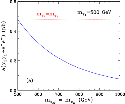
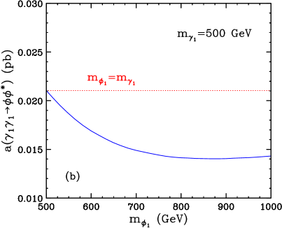
Figure 1: The $a$-term of the annihilation cross-section for (a) $\gamma_{1}\gamma_{1}\rightarrow e^{+}e^{-}$ and (b) $\gamma_{1}\gamma_{1}\rightarrow\phi\phi^{\ast}$, as a function of the mass of the $t$-channel particle(s). We fix the LKP mass at $m_{\gamma_{1}}=500$ GeV and vary (a) the KK lepton mass $m_{e_{R1}}=m_{e_{L1}}$ or (b) the KK Higgs boson mass $m_{\phi_{1}}$. The blue solid lines are the exact results (22) and (26), while the red dotted lines correspond to the approximations (23) and (27).

For the Higgs boson final states we get

$$a = \sum_{i}\frac{2\pi\alpha_{1}^{2}Y_{\phi_{i}}^{4}}{9m_{\gamma_{1}}^{2}}\left(\frac{11m_{\gamma_{1}}^{4}-2m_{\gamma_{1}}^{2}m_{\phi_{i}}^{2}+3m^{4}_{\phi_{i}}}{(m_{\gamma_{1}}^{2}+m_{\phi_{i}}^{2})^{2}}\right)$$ (26)

$$\approx \sum_{i}\frac{2\pi\alpha_{1}^{2}Y_{\phi_{i}}^{4}}{3m_{\gamma_{1}}^{2}}=\frac{4\pi\alpha_{1}^{2}Y_{\phi}^{4}}{3m_{\gamma_{1}}^{2}}\ ,$$ (27)

$$b = -\sum_{i}\frac{\pi\alpha_{1}^{2}Y_{\phi_{i}}^{4}}{108m_{\gamma_{1}}^{2}}\left(\frac{121m_{\gamma_{1}}^{8}+140m_{\gamma_{1}}^{6}m_{\phi_{i}}^{2}-162m_{\gamma_{1}}^{4}m_{\phi_{i}}^{4}+60m_{\gamma_{1}}^{2}m_{\phi_{i}}^{6}-15m_{\phi_{i}}^{8}}{(m_{\gamma_{1}}^{2}+m_{\phi_{i}}^{2})^{4}}\right)$$ (28)

$$\approx -\sum_{i}\frac{\pi\alpha_{1}^{2}Y^{2}_{\phi_{i}}}{12m_{\gamma_{1}}^{2}}=-\frac{\pi\alpha_{1}^{2}Y^{2}_{\phi}}{6m_{\gamma_{1}}^{2}}\ .$$ (29)

In the limit where all KK masses are the same (the second line in each formula above), we recover the result of [6]. Notice the tremendous simplification which arises as a result of the mass degeneracy assumption. In Fig. 1 we show the $a$ terms of the annihilation cross-section for two processes: (a) $\gamma_{1}\gamma_{1}\rightarrow e^{+}e^{-}$ and (b) $\gamma_{1}\gamma_{1}\rightarrow\phi\phi^{\ast}$, as a function of the mass of the $t$-channel particle(s). We fix the LKP mass at $m_{\gamma_{1}}=500$ GeV and vary (a) the KK lepton mass $m_{e_{R1}}=m_{e_{L1}}$ or (b) the KK Higgs boson mass $m_{\phi_{1}}$. The blue solid lines are the exact results (22) and (26), while the red dotted lines correspond to the approximations (23) and (27) in which the mass difference between the $t$-channel particles and the LKP has been neglected. We see that the approximations (23) and (27) can result in a relatively large error, whose size depends on the actual mass splitting of the KK particles. This is why in our code we keep all individual mass dependencies.

Another difference between our analysis and that of Ref. [6] is that here we shall use a temperature-dependent $g_{\ast}$ function as defined in (6). The relevant value of $g_{\ast}$ which enters the answer for the LKP relic density (12) is $g_{\ast}(T_{F})$, where $T_{F}=m_{\gamma_{1}}/x_{F}$ is the freeze-out temperature. In Fig. 2a we show a plot of $g_{\ast}(T_{F})$ as a function of $R^{-1}$ in MUED, while in Fig. 2b we show the corresponding values of $x_{F}$. In Fig. 2a one can clearly see the jumps in $g_{\ast}$ when crossing the $b\bar{b}$, $W^{+}W^{-}$, $ZZ$ and $hh$ thresholds (from left to right). The $t\bar{t}$ threshold is further to the right, outside the plotted range. As we shall see below, cosmologically interesting values of $\Omega h^{2}$ are obtained for $R^{-1}$ below 1 TeV, where $g_{\ast}(T_{F})=86.25$, since we are below the $W^{+}W^{-}$ threshold. The analysis of Ref. [6] assumed a constant value of $g_{\ast}=92$, which is only valid between the $W^{+}W^{-}$ and $ZZ$ thresholds.

Figure 2: The quantities (a) $g_{\ast}(T_{F})$ and (b) $x_{F}$ as a function of $R^{-1}$ in MUED.

The expert reader has probably noticed from Fig. 2b that the values of $x_{F}$ which we obtain in MUED are somewhat larger than the $x_{F}$ values one would have in typical SUSY models. This is due to the effect of coannihilations, which increase $g_{eff}$ (see Fig. 5c below) and therefore $x_{F}$, in accordance with (15).

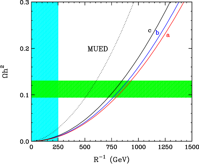
Figure 3: Relic density of the LKP as a function of $R^{-1}$ in the Minimal UED model. The (red) line marked “a” is the result from considering $\gamma_{1}\gamma_{1}$ annihilation only, following the analysis of Ref. [6], assuming a degenerate KK mass spectrum. The (blue) line marked “b” repeats the same analysis, but uses $T$-dependent $g_{\ast}$ according to (6) and includes the relativistic correction to the $b$-term (19). The (black) line marked “c” relaxes the assumption of KK mass degeneracy, and uses the actual MUED mass spectrum. The dotted line is the result from the full calculation in MUED, including all coannihilation processes, with the proper choice of masses. The green horizontal band denotes the preferred WMAP region for the relic density $0.094<\Omega_{CDM}h^{2}<0.129$. The cyan vertical band delineates values of $R^{-1}$ disfavored by precision data.

We are now in a position to discuss our main result in MUED. In Fig. 3 we show the LKP relic density as a function of $R^{-1}$ in the Minimal UED model. We show the results from several analyses, each under different assumptions, in order to illustrate the effect of each assumption. We first show several calculations for the academic case of no coannihilations. The three solid lines in Fig. 3 account only for the $\gamma_{1}\gamma_{1}$ process. The (red) line marked “a” recreates the analysis of Ref. [6], assuming a degenerate KK mass spectrum. The (blue) line marked “b” repeats the same analysis, but uses $T$-dependent $g_{\ast}$ according to (6) and includes the relativistic correction to the $b$-term (19). The (black) line marked “c” further relaxes the assumption of KK mass degeneracy, and uses the actual MUED mass spectrum.

Comparing lines “a” and “b”, we see that, as already anticipated from Fig. 2a, accounting for the $T$ dependence in $g_{\ast}$ has the effect of lowering $g_{\ast}(x_{F})$, $\sigma_{eff}(x_{F})$, and correspondingly, increasing the prediction for $\Omega h^{2}$. This, in turns, lowers the preferred mass range for $\gamma_{1}$. Next, comparing lines “b” and “c”, we see that dropping the mass degeneracy assumption has a similar effect on $\sigma_{eff}(x_{F})$ (see Fig. 1), and further increases the calculated $\Omega h^{2}$. This can be easily understood from the $t$-channel mass dependence exhibited in (22) and (26). The $t$-channel masses appear in the denominator, and they are by definition larger than the LKP mass. Therefore, using their actual values can only decrease $\sigma_{eff}$ and increase $\Omega h^{2}$.

The dotted line in Fig. 3 is the result from the full calculation in MUED, including all coannihilation processes, with the proper choice of masses. The green horizontal band denotes the preferred WMAP region for the relic density $0.094<\Omega_{CDM}h^{2}<0.129$. The cyan vertical band delineates values of $R^{-1}$ disfavored by precision data [41]. We see that according to the full calculation, the cosmologically ideal mass range is $m_{\gamma_{1}}\sim 500-600$ GeV, when $\gamma_{1}$ accounts for all of the dark matter in the Universe. This range is somewhat lower than earlier studies have indicated, mostly due to the effects discussed above. Since the MUED model will be our reference point for the investigations in Section 5, the dotted line from Fig. 3 will be appearing in all subsequent plots in Section 5 below.

5 Relative Weight of Different Coannihilation Processes

As we already explained in the Introduction, the assumptions behind the MUED model can be easily relaxed by allowing nonvanishing boundary terms at the scale $\Lambda$. This would modify the KK spectrum and correspondingly change our prediction for the KK relic density from the previous section. Our code is able to handle such more general cases with ease, since we use as inputs the physical KK masses. In order to gain some insight into the cosmology of such non-minimal scenarios, we have studied the effects of varying the $n=1$ KK masses one at a time. The change in any given KK mass will not only enhance or suppress the related coannihilation processes, but also impact any other cross-sections which happen to have a dependence on the mass parameter being varied. Thus the results in this section may allow one to judge the importance of each individual coannihilation process, and anticipate the answer for $\Omega h^{2}$ in non-minimal models.

We have classified the discussion in this section by particle types. Section 5.1 contains our results for the annihilation processes with KK leptons. Many of our results have already appeared in Ref. [6]. The new element here is the discussion of $\ell_{L1}$ coannihilations. The results presented in Sections 5.2 and 5.3 are completely new – there we investigate the coannihilation effects with strongly interacting KK modes and electroweak gauge bosons and/or Higgs bosons, respectively.

5.1 Effects due to coannihilations with KK leptons

We begin with a discussion of $\gamma_{1}$ coannihilations with the $n=1$ $SU(2)_{W}$-singlet leptons $\ell_{R1}$ and the $n=1$ $SU(2)_{W}$-doublet leptons $\ell_{L1}$. One might expect that those processes will be important, since the KK leptons receive relatively small one-loop mass corrections. For example, in the Minimal UED model $\Delta_{\ell_{R1}}\sim 1\%$ and $\Delta_{\ell_{L1}}\sim 3\%$. It is natural to expect that this degeneracy might persist in non-minimal models as well.

Our approach is as follows. Since we keep separate values for the KK masses, when we start varying any one of them, we have to somehow fix the remainder of the KK mass spectrum. We choose to use MUED as our reference model, hence the masses which are not being varied, will be fixed according to their MUED values. We shall still show results for $\Omega h^{2}$ as a function of $R^{-1}$, but for various fixed values of the corresponding mass splitting $\Delta_{i}$ defined in eq. (21). We shall also always display the reference MUED model line, for which, of course, $\Delta_{i}$ takes its MUED value.

Figure 4: Coannihilation effects of (a) 1 generation or (b) 3 generations of singlet KK leptons. The lines show the LKP relic density as a function of $R^{-1}$, for several choices of the mass splitting $\Delta_{\ell_{R1}}$ between the LKP and the $SU(2)_{W}$-singlet KK fermions $\ell_{R1}$. In each case we use the MUED spectrum to fix the masses of the remaining particles, and then vary the $\ell_{R1}$ mass by hand. The solid lines from top to bottom in both (a) and (b) correspond to $\Delta_{e_{R1}}=0,0.3,0.1$. The dotted line is the nominal UED case from Fig. 3.

Our first example is shown in Fig. 4, where we illustrate the size of the coannihilation effects for (a) 1 generation or (b) 3 generations of degenerate singlet KK leptons $\ell_{R1}$. The lines show the LKP relic density as a function of $R^{-1}$, for several choices of the mass splitting $\Delta_{\ell_{R1}}$ between the LKP and the $SU(2)_{W}$-singlet KK fermions $\ell_{R1}$. The solid lines from top to bottom in both (a) and (b) correspond to $\Delta_{e_{R1}}=0,0.3,0.1$, and the dotted line is the nominal UED case from Fig. 3, for which $\Delta_{\ell_{R1}}=0.01$. As expected, all lines follow the general trend of Fig. 3. In accord with the observations of Ref. [6], we see that $\ell_{R1}$ coannihilations increase the prediction for $\Omega h^{2}$. Such a behavior may seem peculiar at first sight, since in supersymmetry one finds the opposite phenomenon — coannihilations with sleptons tend to reduce the SUSY WIMP relic density. The difference between the two cases can be intuitively understood as follows. In SUSY, the cross-section for the main annihilation channel ($\tilde{\chi}^{0}_{1}\tilde{\chi}^{0}_{1}\to f\bar{f}$) is helicity suppressed, but the coannihilation processes are not. Adding coannihilations therefore can only increase the effective cross-section (9) and correspondingly decrease $\Omega h^{2}$. In contrast, in UED the main annihilation channel ($\gamma_{1}\gamma_{1}\to f\bar{f}$) is already of normal strength. The effect of coannihilations can be easily guessed only if the additional processes have either much weaker or much stronger interactions. In the case of $\ell_{R1}$, however, the additional processes are of the same order (both $\gamma_{1}$ and $\ell_{R1}$ have hypercharge interactions only) and the sign of the coannihilation effect depends on the detailed balance of numerical factors, which will be illustrated in Fig. 5 and discussed in more detail below.

The spread in the lines in Fig. 4 is indicative of the importance of the coannihilations. Comparing Fig. 4a and Fig. 4b, we see that in the case of three generations, the effects are magnified correspondingly. A similar conclusion was reached in Ref. [6].

Notice the peculiar ordering of the lines corresponding to different $\Delta_{\ell_{R1}}$. With respect to variations of $\Delta_{\ell_{R1}}$, the maximum possible value of $\Omega h^{2}$ is obtained for $\Delta_{\ell_{R1}}\to 0$, where the effect of coannihilations is maximal. Then, as we increase the mass splitting between $\ell_{R1}$ and $\gamma_{1}$, at first $\Omega h^{2}$ decreases (see the sequence of $\Delta_{\ell_{R1}}=0$, $\Delta_{\ell_{R1}}=0.01$ and $\Delta_{\ell_{R1}}=0.1$) but then starts increasing again and the $\Omega h^{2}$ values that we get for $\Delta_{\ell_{R1}}=0.3$ are slightly larger than those for $\Delta_{\ell_{R1}}=0.1$. This behavior can be seen more clearly from Fig. 5a, where we vary the mass of the $SU(2)_{W}$-singlet KK electron $e_{R1}$ and plot $\Omega h^{2}$ versus $\Delta_{e_{R1}}$ for a fixed $R^{-1}=500$ GeV.

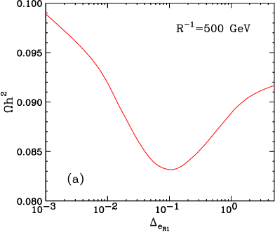
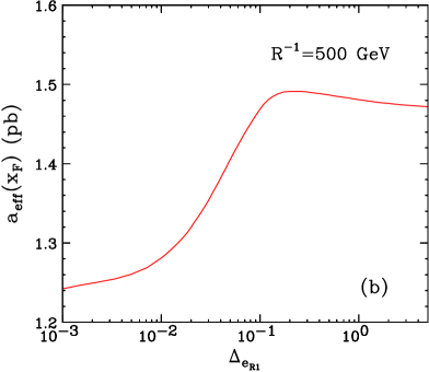
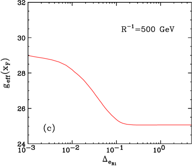
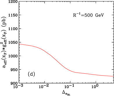
Figure 5: Plots of various quantities entering the LKP relic density computation, as a function of the mass splitting $\Delta_{e_{R1}}$ between the LKP and the $SU(2)_{W}$-singlet KK electron, for $R^{-1}=500$ GeV in MUED. (a) Relic density, (b) $a_{eff}(x_{F})$, (c) $g_{eff}(x_{F})$ and (d) $a_{eff}(x_{F})g^{2}_{eff}(x_{F})$.

The interesting behavior of $\Omega h^{2}$ exhibited in Fig. 5a can be understood in terms of the $m_{\ell_{R1}}$ dependence of the effective annihilation cross-section (9) which is dominated by its $a$-term (17). Both $\sigma_{eff}$ and $a_{eff}$ are functions of $x$, but for the purposes of our discussion here it is sufficient to concentrate on the fixed value $x=x_{F}$ which dominates the integrals (13) and (14). We plot $a_{eff}(x_{F})$ as a function of $\Delta_{e_{R1}}$ in Fig. 5b. We see that $a_{eff}(x_{F})$ exhibits exactly the opposite dependence to $\Omega h^{2}$, and in particular, has an analogous local extremum at $\Delta_{e_{R1}}\sim 0.1$. Therefore, in order to understand qualitatively the behavior of $\Omega h^{2}$, we only need to concentrate on $a_{eff}(x_{F})$.

Let us start with the large $\Delta_{e_{R1}}$ region in Fig. 5b. The $SU(2)_{W}$-singlet KK electron $e_{R1}$ is then too heavy to participate in any relevant coannihilation processes. The effective cross-section (9) then receives no contributions from processes with $e_{R1}$. Nevertheless, the mass of $e_{R1}$ enters $\sigma_{eff}$ through the cross-section for the process $\gamma_{1}\gamma_{1}\to e^{+}e^{-}$ (see eqs. (22) and (24)). Then as we lower $m_{e_{R1}}$, $\sigma(\gamma_{1}\gamma_{1}\to e^{+}e^{-})$ is increased and this leads to a corresponding increase in $a_{eff}$ as seen in Fig. 5b. This trend continues down to $\Delta_{e_{R1}}\sim 0.1$, where coannihilations with $e_{R1}$ start becoming relevant. This can be seen in Fig. 5c, where we plot $g_{eff}(x_{F})$ as a function of $\Delta_{e_{R1}}$. From its defining equation (10) we see that $g_{eff}(x)$ starts to deviate from a constant only when the exponential terms (which signal the turning on of coannihilations) become non-negligible. The exponential terms are all positive and increase $g_{eff}$. At the same time, there are new cross-section terms entering the sum for $\sigma_{eff}$, so we expect the numerator in (9) to increase as well. This is confirmed in Fig. 5d, where we plot the numerator of (9) simply as $a_{eff}(x_{F})g^{2}_{eff}(x_{F})$. From Figs. 5c and 5d we see that both the numerator and the denominator of (17) increase at low $\Delta_{e_{R1}}$, and so it is a priori unclear how their ratio will behave with $\Delta_{e_{R1}}$. In this particular case, $g_{eff}$ wins, and $a_{eff}(x_{F})$ is effectively decreased as a result of turning on the coannihilations with $e_{R1}$. This feature was also observed in Ref. [6].

Figure 6: The same as Fig. 4 but illustrating the effects of varying the $SU(2)_{W}$-doublet KK electron mass. From top to bottom, the solid lines show $\Omega h^{2}$ as a function of $R^{-1}$, for $\Delta_{e_{L1}}=0.01,0.001,0$. The dotted line is the nominal UED case from Fig. 3.

We are now in position to repeat the same analysis, but for the case of the $SU(2)_{W}$-doublet KK leptons $\ell_{L1}$. In Fig. 6, in complete analogy to Fig. 4, we illustrate the effects on the relic density from varying the $SU(2)_{W}$-doublet KK electron mass. From top to bottom, the solid lines show $\Omega h^{2}$ as a function of $R^{-1}$, for $\Delta_{e_{L1}}=0.01,0.001,0$. The dotted line is again the MUED reference model. We see that the case of $SU(2)_{W}$-doublet KK leptons is different. Unlike $\ell_{R1}$, they have weak interactions, and the extra terms which they bring into the sum (9) are larger than the main annihilation channel. The increase in $g_{eff}$ is similar as before. As a result, this time the increase in the numerator of (9) wins, and the net effect is to increase the effective annihilation cross-section. This leads to a reduction in the predicted value for the relic density, as evidenced from Fig. 6. Notice how the decrease in $\Omega h^{2}$ is monotonic with $\Delta_{e_{L1}}$.

Another difference between $\ell_{R1}$ and $\ell_{L1}$ coannihilations is revealed by comparing the case of 1 generation (panels (a) in Figs. 4 and 6) and 3 generations (panels (b) in Figs. 4 and 6). We see that for $SU(2)_{W}$ singlets, the coannihilations are more prominent for the case of 3 generations, while for $SU(2)_{W}$ doublets, it is the opposite. This is due to the different number of degrees of freedom contributed to $g_{eff}$ in each case, which shifts the delicate balance between the numerator and denominator of (9), as discussed above.

5.2 Effects due to coannihilations with KK quarks and KK gluons

We will now consider coannihilation effects with colored KK particles (KK quarks and KK gluons). Since they couple strongly, we expect on general grounds that the effective annihilation cross-sections will be enhanced, and the preferred range of the LKP mass will correspondingly be shifted higher.

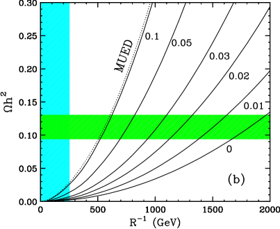
Figure 7: The same as Figs. 4(b) and 6(b), but for the case of KK quarks. Each solid line is labeled by the value of (a) $\Delta_{q_{R1}}$ or (b) $\Delta_{q_{L1}}$ used. The dotted line is the nominal UED case from Fig. 3.

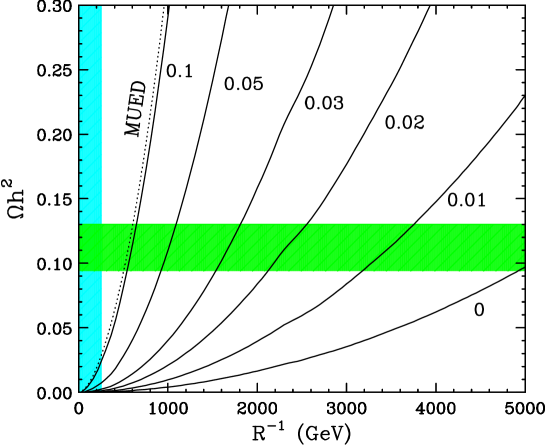
Figure 8: The same as Fig. 7, but for the case of varying the KK gluon mass. The lines are labeled by the value of $\Delta_{g_{1}}$. The dotted line is the nominal UED case from Fig. 3.

These expectations are confirmed by our explicit calculation whose results are shown in Figs. 7 and 8. In Fig. 7 we show the effects on the relic density from varying the masses of all three generations of (a) $SU(2)_{W}$-singlet KK quarks and (b) $SU(2)_{W}$-doublet KK quarks. The solid lines show $\Omega h^{2}$ as a function of $R^{-1}$, and are labeled by the corresponding value of $\Delta_{q_{R1}}$ or $\Delta_{q_{L1}}$ used. As before, the dotted line is the MUED reference model. Comparing the results in Figs. 7a and 7b, we find that the coannihilations with $q_{R1}$ and $q_{L1}$ have very similar effects, as they are both dominated by the strong interactions, which are the same for $q_{R1}$ and $q_{L1}$. Fig. 8 shows the analogous result for the case of varying the KK gluon mass, where the labels now show the values of $\Delta_{g_{1}}$. There is a noticeable distortion of the lines around $R^{-1}\sim 2300$ GeV, which is due to the change in $g_{\ast}$ (see Fig. 2a).

From Figs. 7 and 8 we see that in non-minimal UED models where the colored KK modes happen to exhibit some sort of degeneracy with the LKP, multi-TeV values for $m_{\gamma_{1}}$ are in principle possible. From that point of view, unfortunately, there is no “no-lose” theorem for the LHC or ILC regarding a potential absolute upper bound on the LKP mass.

5.3 Effects due to coannihilations with electroweak KK bosons

We finally show our coannihilation results for the case of electroweak KK gauge bosons ($W^{0}_{1}$ and $W^{\pm}_{1}$) and KK Higgs bosons ($H^{0}_{1}$, $G^{0}_{1}$ and $G^{\pm}_{1}$). The results are displayed in Figs. 9a and 9b, correspondingly. Due to the $SU(2)_{W}$ symmetry, all three $n=1$ KK $W$-bosons are very degenerate, and we have assumed a common parameter $\Delta_{W_{1}}$ for all three. Similarly, the masses of the $n=1$ KK Higgs bosons differ only by electroweak symmetry breaking effects, which we neglect throughout the calculation. We have therefore assumed a common parameter $\Delta_{H}$ for them as well.

Since both the electroweak KK gauge bosons and the KK Higgs bosons have weak interactions, we expect the results to be similar to the case of $SU(2)_{W}$-doublet leptons in the sense that coannihilations would lower the predictions for $\Omega h^{2}$. This is confirmed by Fig. 9. We observe that the effects from the KK $W$-bosons are actually quite significant, and can push the preferred LKP mass as high as 1.4 TeV.

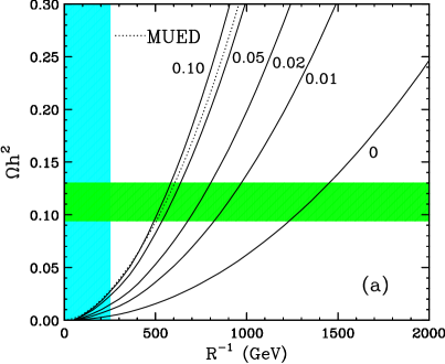
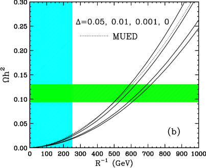
Figure 9: The same as Fig. 8, but illustrating the effect of varying simultaneously the masses of all (a) $SU(2)$ KK gauge bosons and (b) KK Higgs bosons. In (a) the lines are labeled by the value of $\Delta_{W_{1}}$, while in (b) the values of $\Delta_{H}$ are (from top to bottom) $\Delta_{H}=0.05,0.01,0.001,0$. The dotted line is the nominal UED case from Fig. 3.

6 Summary and Conclusions

In this paper we revisited the calculation of the LKP relic density in the scenario of Universal Extra Dimensions. We extended the analysis of Ref. [6] to include all coannihilation processes involving $n=1$ KK partners. This allowed us to predict reliably the preferred mass range for the KK dark matter particle in the Minimal UED model. We found that in order to account for all of the dark matter in the universe, the mass of $\gamma_{1}$ should be within $500-600$ GeV, which is somewhat lower than the range found in [6]. This is due to a combination of several factors. Among the effects which caused our prediction for $\Omega h^{2}$ to go up are the following: we used a lower value of $g_{\ast}$, we kept the individual KK masses in our formulas, and we accounted for the relativistic correction (19). On the other hand, as we saw in Section 5, including the effect of coannihilations with KK particles other than $SU(2)_{W}$-singlet KK leptons, always has the effect of lowering the predicted $\Omega h^{2}$. Finally, the cosmologically preferred range for $\Omega h^{2}$ itself has shifted lower since the publication of [6].

The lower range of preferred values for $R^{-1}$ is good news for collider and astroparticle searches for KK dark matter. It should be kept in mind that it is quite plausible, and in fact very likely, that the dark matter is made up of not one but several different components, in which case the LKP could be even lighter. We should mention that several collider studies [4, 25, 32, 33] have already used an MUED benchmark point with $R^{-1}=500$ GeV, a choice which we now see also happens to be relevant for cosmology.

In Section 5 we also investigated how each class of $n=1$ KK partners impacts the KK relic density. We summarize the observed trends in Fig. 10, where we fix $\Omega h^{2}=0.1$ and then show the required $R^{-1}$ for any given $\Delta_{i}$, for each class of KK particles. We show variations of the masses of one (red dotted) or three (red solid) generations of $SU(2)_{W}$-singlet KK leptons; three generations of $SU(2)_{W}$-doublet leptons (magenta); three generations of $SU(2)_{W}$-singlet quarks (blue) (the result for three generations of $SU(2)_{W}$-doublet quarks is almost identical); KK gluons (cyan) and electroweak KK gauge bosons (green). The circle on each line denotes the MUED values of $\Delta$ and $R^{-1}$.

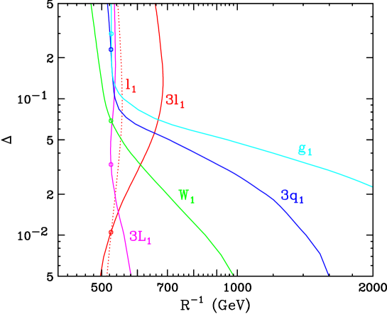
Figure 10: The change in the cosmologically preferred value for $R^{-1}$ as a result of varying the different KK masses away from their nominal MUED values. Along each line, the LKP relic density is $\Omega_{\chi}h^{2}=0.1$. To draw the lines, we first fix the MUED spectrum, and then vary the corresponding KK mass and plot the value of $R^{-1}$ which is required to give $\Omega_{\chi}h^{2}=0.1$. We show variations of the masses of one (red dotted) or three (red solid) generations of $SU(2)_{W}$-singlet KK leptons; three generations of $SU(2)_{W}$-doublet leptons (magenta); three generations of $SU(2)_{W}$-singlet quarks (blue) (the result for three generations of $SU(2)_{W}$-doublet quarks is almost identical); KK gluons (cyan) and electroweak KK gauge bosons (green). The circle on each line denotes the MUED values of $\Delta$ and $R^{-1}$.

Fig. 10 summarizes our results from Section 5. It also provides a quick reference guide for the expected variations in the predicted value of $\Omega h^{2}$ as we move away from the Minimal UED model. For example, it is clear that unlike the case of coannihilations with $\ell_{R1}$, which was considered in [6], coannihilations with all other KK particles will lower the prediction for $\Omega h^{2}$ and correspondingly increase the preferred range of $R^{-1}$. This is due to the larger couplings of those particles. Fig. 10 can also be used to quantitatively estimate the variations in the preferred value of $R^{-1}$ in non-minimal models.

On a final note, in the non-minimal UED model, other neutral KK particles such as $Z_{1}$ can also be dark matter candidates. On dimensional grounds, the relic density is inversely proportional to the square of the LKP mass,

$$\Omega{h^{2}} \sim \frac{g_{1}^{4}}{m_{\gamma_{1}}^{2}}\ ,$$ (30)

$$\Omega{h^{2}} \sim \frac{g_{2}^{4}}{m_{Z_{1}}^{2}}\ .$$ (31)

Due to the larger coupling $g_{2}$ of the $SU(2)_{W}$ gauge interactions, we expect the upper bound on $m_{Z_{1}}$, consistent with WMAP, to be larger than the bound on $m_{\gamma_{1}}$ roughly by a factor of $g^{2}_{2}/g^{2}_{1}\sim 3$. However, in the $Z_{1}$ LKP case, $SU(2)_{W}$ symmetry implies that the charged $W_{1}$ states are almost degenerate with $Z_{1}$, and therefore coannihilations with $W_{1}^{\pm}$ will be very important and will need to be considered. The analysis of the cases of $Z_{1}$ and $H_{1}$ LKP and their detection prospects is currently in progress [71]. The results presented in this paper are also relevant for the case of KK graviton superwimps [72, 73, 74], whose relic density is still determined by the freeze-out of the next-to-lightest KK particle.

In conclusion, dark matter candidates from theories with extra dimensions should be considered on an equal footing with more conventional candidates such as SUSY dark matter or axions. The framework of Universal Extra Dimensions provides a useful playground for gaining some experience about the signals one could expect from extra dimensional dark matter. If extra dimensions have indeed something to do with the dark matter problem, the explicit realization of that idea may look quite differently (see for example [75, 76, 77]), especially if one wants to resolve the radion stabilization problem [78, 79]. Nevertheless, we believe that the methods and insight we developed in this paper will prove useful in more general contexts.

Note added: During the completion of this work we became aware of an analogous calculation done independently by another group [12]. We have compared extensively the formulas for the annihilation cross-sections involving KK quarks, KK leptons and KK gauge bosons, in the limit of degenerate KK masses, as listed in the Appendix. In all considered cases we found perfect agreement.

Appendix A Annihilation Cross-Sections

In this section, we summarize the annihilation cross sections of any pair of $n=1$ KK particles into SM fields in the limit of no electroweak symmetry breaking, as in [6]. In order to render the formulas manageable for publication, in this Appendix we list our results in the limit of equal KK masses. However, in our numerical calculation, we kept different masses for all KK particles, which often leads to enormously complicated analytical expressions. We also assume all SM particles to be massless, since we are working in the limit where we neglect electroweak symmetry breaking (EWSB) effects of order $vR$, where $v$ is the Higgs vacuum expectation value in the SM. All cross-sections are calculated at tree level. All vertices satisfy KK-number conservation and KK-parity since KK-number violating interactions are only induced at the loop level [5]. Some of the cross-sections have already appeared in [6] and we find perfect agreement with those results. We define a few constants below which are commonly used in our formulas for the cross-sections.

$$g_{1} = \frac{e}{c_{w}}\ ,$$ (A.1)

$$g_{2} = \frac{e}{s_{w}}\ ,$$ (A.2)

$$g_{Z} = \frac{e}{2s_{w}c_{w}}\ ,$$ (A.3)

$$\beta = \sqrt{1-\frac{4m^{2}}{s}}\ ,$$ (A.4)

$$L = \log\left(\frac{1-\beta}{1+\beta}\right)=-2\tanh^{-1}\beta\ .$$ (A.5)

Here $g_{1}$, $g_{2}$ and $g_{3}$ are the gauge couplings of $U(1)_{Y}$, $SU(2)_{W}$ and $SU(3)$. $\beta$ is the velocity of the incoming KK particle in the annihilation process. Notice that $L$ is negative since $0<\beta<1$. $m$ is the KK mass which for the purposes of this appendix is the same for all KK particles, $e$ is the electric charge and $c_{w}$ and $s_{w}$ are the cosine and sine of the Weinberg angle in the SM. Table 1 provides a quick reference guide for the different process types.

	Gauge bosons	Leptons	Quarks	Higgses
Gauge bosons	A.2
Leptons	A.3	A.1
Quarks	A.3	A.5	A.4
Higgses	A.7	A.8	A.8	A.6

Table 1: A guide to the formulas in the Appendix. Each box in the table corresponds to a particular type of an initial state. The entry points to the section in the Appendix where the corresponding annihilation cross-sections can be found. Here “gauge bosons” include EW KK gauge bosons ($W_{1}^{\pm}$, $Z_{1}$ and $\gamma_{1}$) and the KK gluon ($g_{1}$). “Higgses” stands for the KK Higgs ($H_{1}$) and KK Goldstone bosons ($G_{1}^{\pm}$ and $G_{1}$). Leptons contain both $SU(2)_{W}$-singlet KK leptons ($\ell_{R1}$) and $SU(2)_{W}$-doublet KK leptons ($\ell_{L1}$ and $\nu_{\ell_{1}}$). Quarks include both $SU(2)_{W}$-doublet KK quarks ($q_{R1}$) and $SU(2)_{W}$-singlet KK quarks ($q_{L1}$).

A.1 Leptons

Coannihilations with $SU(2)_{W}$-singlet KK leptons $\ell_{R1}$ are important since they are expected to be the next-to-lightest KK particles in the Minimal UED model [6, 5]. For fermion final states with $f\neq\ell$, the cross-section is

$$\sigma(\ell_{R1}^{+}{\ell}_{R1}^{-}\rightarrow f\bar{f})\ =\ \frac{N_{c}g_{1}^{4}Y_{\ell}^{2}(Y_{f_{L}}^{2}+Y_{f_{R}}^{2})(s+2m^{2})}{24\pi\beta s^{2}}\ ,$$ (A.6)

where $N_{c}$ is 3 for quarks and 1 for leptons. For cases with the same lepton flavor in the initial and final state, we have

$$\sigma(\ell_{R1}^{+}\ell_{R1}^{-}\rightarrow\ell^{+}\ell^{-}) = \frac{g_{1}^{4}Y_{\ell_{R1}}^{4}(5\beta s+2(2s+3m^{2})L)}{32\pi\beta^{2}s^{2}}$$

$$+ \frac{g_{1}^{4}Y_{\ell_{R1}}^{4}(\beta(4s+9m^{2})+8m^{2}L)}{64\pi m^{2}\beta^{2}s}$$

$$+ \frac{g_{1}^{4}Y_{\ell_{R1}}^{2}(Y_{\ell_{R}}^{2}+Y_{\ell_{L}}^{2})(s+2m^{2})}{24\pi\beta s^{2}}\ ,$$

$$\sigma(\ell_{R1}^{\pm}\ell_{R1}^{\pm}\rightarrow\ell^{\pm}\ell^{\pm})\ =\ \frac{g_{1}^{4}Y_{\ell}^{4}(-m^{2}(4s-5m^{2})L-\beta s(2s-m^{2}))}{32\pi\beta^{2}s^{2}m^{2}}\ ,$$ (A.8)

$$\sigma(\ell_{R1}^{\pm}{\ell^{\prime}}_{R1}^{\pm}\rightarrow\ell^{\pm}{\ell^{\prime}}^{\pm})\ =\ \frac{g_{1}^{4}Y_{\ell}^{4}(4s-3m^{2})}{64\pi\beta sm^{2}}\ ,$$ (A.9)

$$\sigma(\ell_{R1}^{\pm}{\ell^{\prime}}_{R1}^{\mp}\rightarrow\ell^{\pm}{\ell^{\prime}}^{\mp})\ =\ \frac{g_{1}^{4}Y_{\ell}^{4}(\beta(4s+9m^{2})+8m^{2}L)}{64\pi\beta^{2}sm^{2}}\ ,$$ (A.10)

where $\ell$ and $\ell^{\prime}$ are the leptons from different families. For the remaining final states we get

$$\sigma(\ell_{R1}^{+}{\ell}_{R1}^{-}\rightarrow\phi\phi^{*})\ =\ \frac{g_{1}^{4}Y_{\ell}^{2}Y_{\phi}^{2}(s+2m^{2})}{48\pi\beta s^{2}}\ ,$$ (A.11)

$$\sigma(\ell_{R1}^{+}{\ell}_{R1}^{-}\rightarrow B_{0}B_{0})\ =\ \frac{g_{1}^{4}Y_{\ell}^{4}(2(s^{2}+4m^{2}s-8m^{4})-\beta s(s+4m^{2}))}{8\pi\beta^{2}s^{3}}\ .$$ (A.12)

Our results, (A.6-A.12), exactly agree with (C.1) - (C.8) from [6].

The cross-sections among left handed fermions are somewhat complicated since they involve $SU(2)_{W}$ gauge bosons as well as $U(1)_{Y}$ gauge bosons. For KK neutrinos we find

$$\sigma(\nu_{\ell 1}\bar{\nu}_{\ell 1}\rightarrow f\bar{f})\ =\ \frac{N_{c}g_{Z}^{2}(\bar{g}_{L}^{2}+\bar{g}_{R}^{2})(s+2m^{2})}{24\pi\beta s^{2}}\ ,$$ (A.13)

$$\sigma(\nu_{\ell 1}\bar{\nu}_{\ell 1}\rightarrow\phi\phi^{*})\ =\ \frac{g_{\phi}^{2}g_{Z}^{2}(s+2m^{2})}{48\pi\beta s^{2}}\ ,$$ (A.14)

$$\sigma(\nu_{\ell 1}\bar{\nu}_{\ell 1}\rightarrow ZZ)\ =\ \frac{g_{Z}^{4}((8m^{4}-s^{2}-4m^{2}s)L-\beta s(s+4m^{2}))}{8\pi\beta^{2}s^{3}}\ ,$$ (A.15)

$$\sigma(\nu_{\ell 1}\bar{\nu}_{\ell 1}\rightarrow W^{+}W^{-}) = -\frac{5g_{2}^{4}(s+2m^{2})}{96\pi\beta s^{2}}+\frac{g_{2}^{4}(\beta s-2m^{2}L)}{32\pi\beta^{2}s^{2}}$$ (A.16)

$$- \frac{g_{2}^{4}(\beta(s+4m^{2})+(s+2m^{2})L)}{32\pi\beta^{2}s^{2}}\ ,$$

$$\sigma(\nu_{\ell 1}\nu_{\ell 1}\rightarrow\nu_{\ell}\nu_{\ell})\ =\ \frac{g_{Z}^{4}(\beta s(2s-m^{2})-m^{2}(4s-5m^{2})L)}{32\pi\beta^{2}s^{2}m^{2}}\ ,$$ (A.17)

$$\sigma(\nu_{\ell 1}\nu_{\ell^{\prime}1}\rightarrow\nu_{\ell}\nu_{\ell^{\prime}})\ =\ \frac{g_{Z}^{4}(4s-3m^{2})}{64\pi\beta sm^{2}}\ ,$$ (A.18)

$$\sigma(\nu_{\ell 1}\bar{\nu}_{\ell^{\prime}1}\rightarrow\nu_{\ell}\bar{\nu}_{\ell^{\prime}})\ =\ \frac{g_{Z}^{4}(\beta(4s+9m^{2})+8m^{2}L)}{64\pi\beta^{2}sm^{2}}\ ,$$ (A.19)

$$\sigma(\nu_{\ell 1}\bar{\nu}_{\ell^{\prime}1}\rightarrow\ell^{-}{\ell^{\prime}}^{+})\ =\ \frac{g_{2}^{4}(\beta(4s+9m^{2})+8m^{2}L)}{256\pi\beta^{2}sm^{2}}\ ,$$ (A.20)

$$\sigma(\nu_{\ell 1}\bar{\nu}_{\ell 1}\rightarrow\ell^{+}{\ell}^{-}) = \frac{g_{Z}\hat{g}_{L}^{2}\bar{g}_{L}(5\beta s+2(2s+3m^{2})L)}{32\pi\beta^{2}s^{2}}$$ (A.21)

$$+\frac{g_{Z}^{2}(\bar{g}_{L}^{2}+\bar{g}_{R}^{2})(s+2m^{2})}{24\pi\beta s^{2}}+\frac{\hat{g}_{L}^{4}(\beta(4s+9m^{2})+8m^{2}L)}{64\pi m^{2}\beta^{2}s}\ .$$

Here $\bar{g}_{L(R)}=\frac{e}{s_{w}c_{w}}\left(T^{3}-Q_{f}s_{w}^{2}\right)$, $\hat{g}_{L}=g_{Z}$ for neutrinos and $\hat{g}_{L}=g_{2}/\sqrt{2}$ for charged leptons. $g_{\phi}=\frac{e}{s_{w}c_{w}}\left(T^{3}-Q_{\phi}s_{w}^{2}\right)$ with $Q_{\phi}=1$ for the upper entry in the Higgs doublet and $Q_{\phi}=0$ for the lower entry. Since we ignore EWSB, all gauge bosons have transverse polarizations only. $\phi$ represents either a charged Higgs boson ($\phi_{u}$, isospin $\frac{1}{2}$) or a neutral Higgs boson ($\phi_{d}$, isospin $-\frac{1}{2}$).

The previous results allow us to immediately obtain

$$\sigma(\nu_{\ell 1}\bar{\nu}_{\ell 1}\rightarrow\phi\phi^{*}) = \sigma(\ell_{L1}^{+}\ell_{L1}^{-}\rightarrow\phi\phi^{*})\ ,$$

$$\sigma(\nu_{\ell 1}\bar{\nu}_{\ell 1}\rightarrow ZZ) = \sigma(\ell_{L1}^{+}{\ell}_{L1}^{-}\rightarrow ZZ+Z\gamma+\gamma\gamma)\ ,$$

$$\sigma(\nu_{\ell 1}\bar{\nu}_{\ell 1}\rightarrow W^{+}W^{-}) = \sigma(\ell_{L1}^{+}\ell_{L1}^{-}\rightarrow W^{+}W^{-})\ ,$$

$$\sigma(\nu_{\ell 1}\nu_{\ell 1}\rightarrow\nu_{\ell}\nu_{\ell}) = \sigma(\ell_{L1}^{\pm}\ell_{L1}^{\pm}\rightarrow\ell^{\pm}\ell^{\pm})\ ,$$ (A.22)

$$\sigma(\nu_{\ell 1}\nu_{\ell^{\prime}1}\rightarrow\nu_{\ell}\nu_{\ell^{\prime}}) = \sigma(\nu_{\ell 1}\ell^{\prime}_{L1}\rightarrow\nu_{\ell}\ell^{\prime})$$

$$= \sigma(\ell_{L1}^{\pm}{\ell^{\prime}}_{L1}^{\pm}\rightarrow\ell^{\pm}{\ell^{\prime}}^{\pm})\ ,$$

$$\sigma(\nu_{\ell 1}\bar{\nu}_{\ell^{\prime}1}\rightarrow\nu_{\ell}\bar{\nu}_{\ell^{\prime}}) = \sigma(\ell_{L1}^{\pm}{\ell^{\prime}}_{L1}^{\mp}\rightarrow\ell^{\pm}{\ell^{\prime}}^{\mp})\ .$$

For at least one charged KK lepton in the initial state we get

$$\sigma(\ell_{L1}^{+}{\ell}_{L1}^{-}\rightarrow f\bar{f}\,\,or\,\,\ell^{+}_{R}\ell^{-}_{R})\ =\ \frac{N_{c}g^{4}(s+2m^{2})}{24\pi\beta s^{2}}\ ,$$ (A.23)

$$\sigma(\ell_{L1}^{+}{\ell}_{L1}^{-}\rightarrow\nu_{\ell}\bar{\nu}_{\ell}\,\,or\,\,\ell^{+}_{L}\ell^{-}_{L}) = \frac{\hat{g}_{L}^{2}g^{2}(5\beta s+2(2s+3m^{2})L)}{32\pi\beta^{2}s^{2}}$$ (A.24)

$$+ \frac{\hat{g}_{L}^{4}(\beta(4s+9m^{2})+8m^{2}L)}{64\pi m^{2}\beta^{2}s}+\frac{g^{4}(s+2m^{2})}{24\pi\beta s^{2}}\ ,$$

$$\sigma(\ell_{L1}^{-}\bar{\nu}_{L1}\rightarrow f\bar{f}^{\prime})\ =\ \frac{N_{c}g_{2}^{4}(s+2m^{2})}{96\pi\beta s^{2}}\ ,$$ (A.25)

$$\sigma(\ell_{L1}^{-}\bar{\nu}_{L1}\rightarrow\phi^{*}_{u}\phi_{d})\ =\ \frac{g_{2}^{4}(s+2m^{2})}{192\pi\beta s^{2}}\ ,$$ (A.26)

$$\sigma(\ell_{L1}^{-}\bar{\nu}_{L1}\rightarrow W^{-}B_{0})\ =\ \frac{g_{1}^{2}g_{2}^{2}((8m^{4}-s^{2}-4m^{2}s)L-\beta s(s+4m^{2}))}{32\pi\beta^{2}s^{3}}\ ,$$ (A.27)

$$\sigma(\ell_{L1}^{-}\bar{\nu}_{L1}\rightarrow W^{-}W^{0}_{3}) = -\frac{5g_{2}^{4}(s+2m^{2})}{48\pi s^{2}\beta}+\frac{g_{2}^{4}(\beta s-2m^{2}L)}{32\pi s^{2}\beta^{2}}$$ (A.28)

$$- \frac{g_{2}^{4}(\beta(s+4m^{2})+(s+2m^{2})L)}{64\pi s^{2}\beta}+\frac{g_{2}^{4}m^{2}L}{16\pi s^{2}}\ ,$$

$$\sigma(\ell_{L1}^{-}\bar{\nu}_{L1}\rightarrow\ell^{-}\bar{\nu}_{\ell}) = \frac{g_{1}g_{2}^{3}(5\beta s+2(2s+3m^{2})L)}{64\pi\beta^{2}s^{2}(2s_{w}^{2}-1)}$$ (A.29)

$$+ \frac{g_{1}^{2}g_{2}^{2}(\beta(4s+9m^{2})+8m^{2}L)}{64\pi m^{2}\beta^{2}s(2s_{w}^{2}-1)^{2}}+\frac{g_{2}^{4}(s+2m^{2})}{96\pi\beta s^{2}}\ ,$$

$$\sigma(\ell_{L1}^{-}\nu_{L1}\rightarrow\ell^{-}\nu_{\ell}) = \frac{g_{1}g_{2}^{3}(-2m^{2}(4s-5m^{2})L+m^{2}\beta s)}{64\pi\beta^{2}s^{2}m^{2}(2s_{w}^{2}-1)}$$ (A.30)

$$+ \frac{\beta s(4s-3m^{2})}{64\pi\beta^{2}s^{2}m^{2}}\left(\frac{g_{1}^{2}g_{2}^{2}}{(2s_{w}^{2}-1)^{2}}+\frac{g_{2}^{4}}{4}\right)\ ,$$

$$\sigma(\nu_{L1}\ell^{\prime}_{L1}\rightarrow\nu_{\ell^{\prime}}\ell^{-})\ =\ \frac{g_{2}^{4}(4s-3m^{2})}{256\pi m^{2}s\beta}\ ,$$ (A.31)

$$\sigma(\nu_{L1}\ell^{\prime}_{L1}\rightarrow\nu_{\ell}\ell^{\prime-})\ =\ \frac{g_{1}^{2}g_{2}^{2}(4s-3m^{2})}{64\pi m^{2}s\beta(2s_{w}^{2}-1)^{2}}\ ,$$ (A.32)

$$\sigma(\bar{\nu}_{L1}\ell^{\prime}_{L1}\rightarrow\bar{\nu}_{\ell}\ell^{\prime-})\ =\ \frac{g_{1}^{2}g_{2}^{2}(\beta(4s+9m^{2})+8m^{2}L)}{64\pi m^{2}s\beta^{2}(2s_{w}^{2}-1)^{2}}\ ,$$ (A.33)

$$\sigma(\ell_{L1}\bar{\ell}^{\prime}_{L1}\rightarrow\nu_{\ell}\bar{\nu}_{\ell^{\prime}})\ =\ \frac{g_{2}^{4}(\beta(9m^{2}+4s)+8m^{2}L)}{256\pi m^{2}s\beta^{2}}\ ,$$ (A.34)

where $g^{2}=g_{1}^{2}Y_{f}Y_{\ell_{R}}+g_{2}^{2}T_{f}^{3}T^{3}_{\ell_{L}}$. The above cross-sections, (A.13-A.34) are consistent with (B.48) - (B.62) and (B.71) - (B.74) in [6].

For one $SU(2)_{W}$-singlet KK lepton and one $SU(2)_{W}$-doublet KK lepton we get

$$\sigma(\ell_{R1}\ell_{L1}\rightarrow\ell\ell)\ =\ \frac{g_{1}^{4}Y^{2}_{e_{L}}Y^{2}_{e_{R}}}{64\pi m^{2}s\beta^{2}}\left(8m^{2}L+\beta(9m^{2}+4s)\right)\ ,$$ (A.35)

$$\sigma(\ell_{R1}\bar{\ell}_{L1}\rightarrow\ell\bar{\ell})\ =\ \frac{g_{1}^{4}Y^{2}_{e_{L}}Y^{2}_{e_{R}}}{64\pi m^{2}s\beta}\left(4s-3m^{2}\right)\ .$$ (A.36)

These two formulas have the same structure as $\sigma(\ell_{R1}^{\pm}{\ell^{\prime}}_{R1}^{\pm}\rightarrow\ell^{\pm}{\ell^{\prime}}^{\pm})$ and $\sigma(\ell_{R1}^{\pm}{\ell^{\prime}}_{R1}^{\mp}\rightarrow\ell^{\pm}{\ell^{\prime}}^{\mp})$.

A.2 Gauge bosons

The self-annihilation cross-sections of $\gamma_{1}$ are

$$\sigma(\gamma_{1}\gamma_{1}\rightarrow f\bar{f})\ =\ \frac{N_{c}g_{1}^{4}(Y_{f_{L}}^{4}+Y_{f_{R}}^{4})}{72\pi s^{2}\beta^{2}}\left(-5s(2m^{2}+s)L-7s\beta\right)\ ,$$ (A.37)

$$\sigma(\gamma_{1}\gamma_{1}\rightarrow\phi\phi^{*})\ =\frac{g_{1}^{4}Y_{\phi}^{4}}{12\pi s\beta}\ .$$ (A.38)

These two cross-sections are identical to (A.44) and (A.47) in [6]. For $Z_{1}$ self-annihilation into fermions and Higgs bosons,

$$\sigma(Z_{1}Z_{1}\rightarrow f\bar{f})\ =\ \frac{N_{c}g_{2}^{4}}{1152\pi s^{2}\beta^{2}}\left(-5(2m^{2}+s)L-7s\beta\right)\ ,$$ (A.39)

$$\sigma(Z_{1}Z_{1}\rightarrow\phi\phi^{*})\ =\ \frac{g_{2}^{4}}{192\pi s\beta}\ .$$ (A.40)

The cross-section for the above two processes are obtained from $\sigma(\gamma_{1}\gamma_{1}\rightarrow f\bar{f})$ and $\sigma(\gamma_{1}\gamma_{1}\rightarrow\phi\phi^{*})$ by replacing $g_{1}Y$ with $g_{2}/2$, which corresponds to the $Z$ couplings to SM fermions and Higgs bosons. For the coannihilations of $SU(2)_{W}$ KK bosons into SM gauge bosons, we get

$$\sigma(Z_{1}Z_{1}\rightarrow W^{+}W^{-})\ =\ \frac{g_{2}^{4}}{18\pi m^{2}s^{3}\beta^{2}}\left(12m^{2}(s-2m^{2})L+s\beta(12m^{4}+3sm^{2}+4s^{2})\right),$$ (A.41)

$$\sigma(W^{+}_{1}W^{+}_{1}\rightarrow W^{+}W^{+})\ =\ \frac{g_{2}^{4}}{36\pi m^{2}s^{3}\beta^{2}}\left(12m^{4}(s-2m^{2})L+s\beta(12m^{4}+3sm^{2}+4s^{2})\right),$$ (A.42)

$$\sigma(W^{+}_{1}W^{-}_{1}\rightarrow\gamma\gamma)\ =\ \frac{e^{4}}{36\pi m^{2}s^{3}\beta^{2}}\left(12m^{4}(s-2m^{2})L+s\beta(12m^{4}+3sm^{2}+4s^{2})\right)\ ,$$ (A.43)

$$\sigma(W^{+}_{1}W^{-}_{1}\rightarrow\gamma Z)\ =\ \frac{g_{2}^{2}e^{2}c_{w}^{2}}{18\pi m^{2}s^{3}\beta^{2}}\left(12m^{4}(s-2m^{2})L+s\beta(12m^{4}+3sm^{2}+4s^{2})\right)\ ,$$ (A.44)

$$\sigma(W^{+}_{1}W^{-}_{1}\rightarrow ZZ)\ =\ \frac{g_{2}^{4}c_{w}^{4}}{36\pi m^{2}s^{3}\beta^{2}}\left(12m^{4}(s-2m^{2})L+s\beta(12m^{4}+3sm^{2}+4s^{2})\right)\ .$$ (A.45)

We see that the above five cross-sections contain similar expressions up to overall factors due to the gauge structure of $SU(2)_{W}\times U(1)_{Y}$. For $W_{1}^{\pm}$ annihilation into other final states, we have

$$\sigma(W^{+}_{1}W^{-}_{1}\rightarrow f\bar{f})\ =\ \frac{-N_{c}g_{2}^{4}}{576\pi s^{2}\beta^{2}}\left((12m^{2}+5s)L+2\beta(4m^{2}+5s)\right)\ ,$$ (A.46)

$$\sigma(W^{+}_{1}W^{-}_{1}\rightarrow W^{+}W^{-})\ =\ \frac{g_{2}^{4}}{18\pi m^{2}s^{2}\beta^{2}}\left(2m^{2}(3m^{2}+2s)L+\beta(11m^{4}+5sm^{2}+2s^{2})\right)\ ,$$ (A.47)

$$\sigma(W^{+}_{1}W^{-}_{1}\rightarrow\phi\phi^{*})\ =\ \frac{g_{2}^{4}(s-m^{2})}{144\pi s^{2}\beta}\ .$$ (A.48)

These three cross-sections are different since they involve $s$-channel $Z$ diagrams. For $\gamma_{1}Z_{1}$ and $\gamma_{1}W^{-}_{1}$ into fermions we can recycle $\sigma(\gamma_{1}\gamma_{1}\rightarrow f\bar{f})$ and obtain

$$\sigma(\gamma_{1}Z_{1}\rightarrow f\bar{f})\ =\ \frac{-N_{c}g_{1}^{2}g_{2}^{2}Y_{f}^{2}}{288\pi s^{2}\beta^{2}}\left(5(2m^{2}+s)L+7s\beta\right)\ ,$$ (A.49)

$$\sigma(\gamma_{1}W^{-}_{1}\rightarrow f\bar{f^{\prime}})\ =\ \frac{-N_{c}g_{1}^{2}g_{2}^{2}Y_{f}^{2}}{144\pi s^{2}\beta^{2}}\left(5(2m^{2}+s)L+7s\beta\right)\ .$$ (A.50)

For the annihilation of two different KK gauge bosons into Higgs bosons we have

$$\sigma(\gamma_{1}Z_{1}\rightarrow\phi\phi^{*})\ =\ \frac{g_{1}^{2}g_{2}^{2}}{192\pi s\beta}\ ,$$ (A.51)

$$\sigma(\gamma_{1}W^{-}_{1}\rightarrow\phi_{d}\phi_{u}^{*})\ =\ \frac{g_{1}^{2}g_{2}^{2}}{96\pi s\beta}\ ,$$ (A.52)

$$\sigma(Z_{1}W^{-}_{1}\rightarrow\phi_{d}\phi_{u}^{*})\ =\ \frac{g_{2}^{4}\beta}{288\pi s}\ ,$$ (A.53)

which can be obtained from $\sigma(\gamma_{1}\gamma_{1}\rightarrow\phi\phi^{*})$. The cross-section for $Z_{1}W^{-}_{1}$ into fermions

$$\sigma(Z_{1}W^{-}_{1}\rightarrow f\bar{f^{\prime}})\ =\ \frac{-N_{c}g_{2}^{4}}{576\pi s^{2}\beta^{2}}\left((14m^{2}+5s)L+\beta(16m^{2}+13s)\right)\ ,$$ (A.54)

has a different structure compared to other fermion final states due to an s-channel $W$ diagram. The cross-sections for $Z_{1}W^{-}_{1}$ into gauge boson final states

$$\sigma(Z_{1}W^{-}_{1}\rightarrow ZW^{-})\ =\ \frac{g_{2}^{4}c_{w}^{2}}{18\pi m^{2}s^{2}\beta^{2}}\left(2m^{2}(3m^{2}+2s)L+\beta(11m^{4}+5sm^{2}+2s^{2})\right)\ ,$$ (A.55)

$$\sigma(Z_{1}W^{-}_{1}\rightarrow\gamma W^{-})\ =\ \frac{e^{2}g_{2}^{2}}{18\pi m^{2}s^{2}\beta^{2}}\left(2m^{2}(3m^{2}+2s)L+\beta(11m^{4}+5sm^{2}+2s^{2})\right)\ ,$$ (A.56)

can be obtained from $\sigma(W^{+}_{1}W^{-}_{1}\rightarrow W^{+}W^{-})$. For KK gluons we get

$$\sigma(g_{1}g_{1}\rightarrow gg)\ =\ \frac{g_{3}^{4}}{64\pi m^{2}s^{3}\beta^{2}}\left(8m^{2}(s^{2}+3sm^{2}-3m^{4})L+s\beta(34m^{2}+13sm^{2}+8s^{2})\right)\ ,$$ (A.57)

$$\sigma(g_{1}g_{1}\rightarrow q\bar{q})\ =\ \frac{-g_{3}^{4}}{3456\pi s^{2}\beta^{2}}\left(2(20s+49m^{2})L+\beta(72m^{2}+83s)\right)\ ,$$ (A.58)

for which there are no analogous processes. The cross-sections associated with one gluon and one electroweak gauge bosons in the initial state

$$\sigma(g_{1}\gamma_{1}\rightarrow q\bar{q})\ =\ \frac{g_{1}^{2}g_{3}^{2}(Y^{2}_{q_{L}}+Y^{2}_{q_{R}})}{144\pi s^{2}\beta^{2}}\left(-5(2m^{2}+s)L-7s\beta\right)\ ,$$ (A.59)

$$\sigma(g_{1}Z_{1}\rightarrow q\bar{q})\ =\ \frac{g_{2}^{2}g_{3}^{2}}{576\pi s^{2}\beta^{2}}\left(-5(2m^{2}+s)L-7s\beta\right)\ ,$$ (A.60)

$$\sigma(g_{1}W^{-}_{1}\rightarrow q\bar{q^{\prime}})\ =\ \frac{g_{2}^{2}g_{3}^{2}}{288\pi s^{2}\beta^{2}}\left(-5(2m^{2}+s)L-7s\beta\right)\ ,$$ (A.61)

are obtained from $\sigma(\gamma_{1}\gamma_{1}\rightarrow f\bar{f})$, $\sigma(\gamma_{1}Z_{1}\rightarrow f\bar{f})$ and $\sigma(\gamma_{1}W_{1}^{-}\rightarrow f\bar{f^{\prime}})$ by simple coupling replacements and accounting for the additional color factors.

A.3 Fermions and Gauge Bosons

Note that in UED, the Dirac KK fermions are constructed out of two Weyl fermions with the same $SU(2)_{W}\times U(1)_{Y}$ quantum numbers while a Dirac fermion in the Standard Model is made up of two Weyl fermions of different $SU(2)_{W}\times U(1)_{Y}$ quantum numbers. Therefore the couplings of KK fermions to zero mode gauge bosons are vector-like. This difference shows up in processes involving gauge-boson couplings with fermions. For the vertices which involve $n=1$ gauge bosons, we need one KK fermion and one SM fermion in order to conserve KK number. In this case, there is always a projection operator associated with the subscript ($L/R$) of the KK fermion. The annihilation cross-sections with $SU(2)_{W}$-singlet KK fermions and $SU(2)_{W}$ KK gauge bosons ($Z_{1}$ and $W_{1}^{\pm}$) are zero:

$$\sigma(f_{R1}Z_{1}\rightarrow SM) = 0\ ,$$

$$\sigma(f_{R1}W^{\pm}_{1}\rightarrow SM) = 0\ .$$ (A.62)

The cross-section for $SU(2)_{W}$-singlet leptons and $\gamma_{1}$ is

$$\sigma(\gamma_{1}\ell_{R1}^{\pm}\rightarrow B_{0}\ell^{\pm})\ =\ \frac{Y_{\ell}^{4}g_{1}^{4}(-6L-\beta)}{96\pi s\beta^{2}}\ .$$ (A.63)

For a KK quark and $\gamma_{1}$ we have

$$\sigma(q_{1}\gamma_{1}\rightarrow qg)\ =\ \frac{g_{1}^{2}g_{3}^{2}Y_{q_{1}}^{2}}{72\pi s\beta^{2}}\left(-6L-\beta\right)\ .$$ (A.64)

This cross-section is basically the same as $\sigma(\gamma_{1}\ell_{R1}^{\pm}\rightarrow B_{0}\ell^{\pm})$, up to a group factor. In $\sigma(q_{1}\gamma_{1}\rightarrow qg)$, the vertex associated with the SM gluon $g$ contains a Gell-Mann matrix $t_{ij}^{a}$. In the squared matrix element, we then get [80]

$$\sum_{a=1}^{8}\frac{1}{3}\sum_{i,j=1}^{3}t^{a}_{ij}t^{a}_{ji}=\frac{1}{3}\times\frac{4}{3}\times 3=\frac{4}{3}\ .$$ (A.65)

Similarly, for the $SU(2)_{W}$-doublet quarks with $Z_{1}$, we get

$$\sigma(q_{L1}Z_{1}\rightarrow gq)\ =\ \frac{g_{2}^{2}g_{3}^{2}}{288\pi s\beta^{2}}\left(-6L-\beta\right)\ ,$$ (A.66)

by replacing the $g_{1}$ coupling in $\sigma(q_{1}\gamma_{1}\rightarrow qg)$ with $g_{2}/2$. For $W_{1}^{\pm}$, one should use the coupling $g_{2}/\sqrt{2}$ instead:

$$\sigma(q_{L1}W_{1}\rightarrow gq^{\prime})\ =\ \frac{g_{2}^{2}g_{3}^{2}}{144\pi s\beta^{2}}\left(-6L-\beta\right)\ .$$ (A.67)

For the $SU(2)_{W}$-doublet KK leptons and $\gamma_{1}$ or $Z_{1}$, we get

$$\sigma(\ell_{L1}\gamma_{1}\rightarrow\ell_{L}\gamma/Z)\ =\ \frac{g_{1}^{4}}{1536\pi s\beta^{2}s_{w}^{2}}\left(-6L-\beta\right)\ ,$$ (A.68)

$$\sigma(\ell_{L1}Z_{1}\rightarrow\ell_{L}\gamma/Z)\ =\ \frac{g_{2}^{4}}{1536\pi s\beta^{2}c_{w}^{2}}\left(-6L-\beta\right)\ ,$$ (A.69)

$$\sigma(\ell_{L1}\gamma_{1}\rightarrow\nu_{\ell}W)\ =\ \frac{g_{1}^{2}g_{2}^{2}}{768\pi s\beta^{2}}\left(-6L-\beta\right)\ .$$ (A.70)

The last 7 cross-sections have a similar structure since they all have $s$- and $t$-channel diagrams only. For the cross-sections associated with $SU(2)_{W}$-doublet KK leptons and electroweak KK gauge bosons into other final states, we have

$$\sigma(\ell_{L1}Z_{1}\rightarrow\nu_{\ell}W)\ =\ \frac{g_{2}^{4}}{768\pi m^{2}s\beta^{2}}\left(26m^{2}L+\beta(23m^{2}+32s)\right)\ ,$$ (A.71)

$$\sigma(\ell_{L1}W_{1}\rightarrow\nu_{\ell^{\prime}}(\gamma+Z)) = \frac{g_{2}^{4}}{768\pi m^{2}s\beta^{2}c_{w}^{2}}\left(m^{2}(32c_{w}^{2}-6)L\right.$$ (A.72)

$$\hskip 28.45274pt\left.+\beta m(24c_{w}^{2}-1)+32s\beta c_{w}^{2}\right)\ ,$$

$$\sigma(\ell_{L1}W_{1}^{-}\rightarrow\ell_{L}W^{-})\ =\ \frac{g_{2}^{4}}{192\pi m^{2}s\beta^{2}}\left(-3m^{2}L+4s\beta\right)\ ,$$ (A.73)

$$\sigma(\ell_{L1}W_{1}^{+}\rightarrow\ell_{L}W^{+})\ =\ \frac{g_{2}^{4}}{384\pi m^{2}s\beta^{2}}\left(16m^{2}L+\beta(11m^{2}+8s)\right)\ ,$$ (A.74)

$$\sigma(\ell_{L1}W_{1}^{-}\rightarrow\ell_{L}W^{-}) = \sigma(\nu_{\ell 1}W_{1}^{+}\rightarrow\nu_{\ell}W^{+})\ ,$$ (A.75)

$$\sigma(\ell_{L1}W_{1}^{+}\rightarrow\ell_{L}W^{+}) = \sigma(\nu_{\ell 1}W_{1}^{-}\rightarrow\nu_{\ell}W^{-})\ .$$ (A.76)

For KK gluon - KK quark annihilation, we obtain

$$\sigma(g_{1}q_{1}\rightarrow gq)\ =\ \frac{g_{3}^{4}}{846\pi m^{2}s\beta^{2}}\left(24m^{2}L+\beta(25m^{2}+36s)\right)\ .$$ (A.77)

A.4 Quarks

The annihilation cross-section of two KK quarks into SM quarks of different flavor

$$\sigma(q_{1}\bar{q}_{1}\rightarrow q^{\prime}\bar{q}^{\prime})\ =\ \frac{g_{3}^{4}(s+2m^{2})}{54\pi s^{2}\beta}$$ (A.78)

can be obtained from $\sigma(\ell_{R1}^{+}{\ell}_{R1}^{-}\rightarrow f\bar{f})$ by multiplying with the following group factor [80]

$$\frac{1}{3}\frac{1}{3}tr\left(t^{a}t^{b}\right)tr\left(t^{b}t^{a}\right)=\frac{1}{9}C(r)^{2}\delta^{ab}\delta^{ab}=\frac{1}{9}\cdot\frac{1}{4}\cdot 8=\frac{2}{9}.$$ (A.79)

Here $C(r)=1/2$ is the quadratic Casimir operator for the fundamental representation of $SU(3)$. KK quark annihilation into same flavor SM quarks is given by

$$\sigma(q_{1}q_{1}\rightarrow qq)\ =\ \frac{g_{3}^{4}}{432\pi m^{2}s^{2}\beta^{2}}\left(2m^{2}(4s-5m^{2})L+(6s-5m^{2})s\beta\right)\ .$$ (A.80)

In this process, there are three terms in the squared matrix element since we have both $t$- and $u$-channel diagrams. This process also has an analogy with $\sigma(\ell_{R1}^{\pm}\ell_{R1}^{\pm}\rightarrow\ell^{\pm}\ell^{\pm})$. However, each term gets a different group factor. The squares of the $t$- and $u$-channel diagrams get the same factor of $2/9$ but for the cross term we obtain [80]

$$\left(\frac{1}{3}\right)^{2}tr\left(t^{a}t^{b}t^{a}t^{b}\right) = \frac{1}{9}\left(C_{2}(2)-\frac{1}{2}C_{2}(G)\right)tr\left(t^{a}t^{a}\right)$$ (A.81)

$$= \frac{1}{9}\left(\frac{4}{3}-\frac{3}{2}\right)\frac{4}{3}=-\frac{2}{9}=-\frac{2}{27}\ .$$

For $q_{1}\bar{q}_{1}$ annihilation into same flavor SM quarks we get

$$\sigma(q_{1}\bar{q}_{1}\rightarrow q\bar{q})\ =\ \frac{g_{3}^{4}}{864\pi m^{2}s^{2}\beta^{2}}\left(4m^{2}(4s-3m^{2})L+\beta(32m^{4}+33sm^{2}+12s^{2})\right)\ ,$$ (A.82)

which can also be obtained using the analogy to $\sigma(\ell_{R1}^{+}\ell_{R1}^{-}\rightarrow\ell^{+}\ell^{-})$ and taking into account group factors. For the final state with gluons we have

$$\sigma(q_{1}\bar{q}_{1}\rightarrow gg)\ =\ \frac{-g_{3}^{4}}{54\pi s^{3}\beta^{2}}\left(4(m^{4}+4sm^{2}+s^{2})L+s\beta(31m^{2}+7s)\right)\ .$$ (A.83)

For different quark flavors in the initial state, we have

$$\sigma(q_{1}q^{\prime}_{1}\rightarrow qq^{\prime})\ =\ \frac{g_{3}^{4}(4s-3m^{2})}{288\pi m^{2}s\beta}\ ,$$ (A.84)

$$\sigma(q_{1}\bar{q}^{\prime}_{1}\rightarrow q\bar{q}^{\prime})\ =\ \frac{g_{3}^{4}}{288\pi m^{2}s\beta^{2}}\left(8m^{2}L+\beta(9m^{2}+4s)\right)\ .$$ (A.85)

The above two cross-sections can be obtained from $\sigma(\ell_{R1}^{\pm}{\ell^{\prime}}_{R1}^{\pm}\rightarrow\ell^{\pm}{\ell^{\prime}}^{\pm})$ and $\sigma(\ell_{R1}^{\pm}{\ell^{\prime}}_{R1}^{\mp}\rightarrow\ell^{\pm}{\ell^{\prime}}^{\mp})$, correspondingly, by multiplying with the group factor $2/9$. The remaining cross-sections are

$$\sigma(q_{1}\bar{q}^{\prime}_{1}\rightarrow q\bar{q}^{\prime}) = \sigma(u_{R1}\bar{d}_{R1}\rightarrow u\bar{d})\ ,$$

$$= \sigma(u_{R1}d_{L1}\rightarrow ud)\ ,$$

$$= \sigma(u_{R1}u_{L1}\rightarrow uu)\ ,$$

and

$$\sigma(q_{1}q^{\prime}_{1}\rightarrow qq^{\prime}) = \sigma(u_{R1}d_{R1}\rightarrow ud)\ ,$$

$$= \sigma(u_{R1}\bar{d}_{L1}\rightarrow u\bar{d})\ ,$$

$$= \sigma(u_{R1}\bar{u}_{L1}\rightarrow u\bar{u})\ .$$

A.5 Quarks and Leptons

The cross-sections listed below are mediated by $t$- or $u$-channel diagrams with KK gauge bosons. For one KK lepton and one KK quark in the initial state, we get

$$\sigma(\ell_{L1}u_{L1}\rightarrow\ell u)\ =\ \frac{(4g_{1}^{2}Y_{e_{L}}Y_{u_{L}}-g_{2}^{2})^{2}(4s-3m^{2})}{1024\pi m^{2}s\beta}\ ,$$ (A.88)

$$\sigma(\nu_{1}u_{L1}\rightarrow\nu u)\ =\ \frac{(4g_{1}^{2}Y_{e_{L}}Y_{u_{L}}+g_{2}^{2})^{2}(4s-3m^{2})}{1024\pi m^{2}s\beta}\ ,$$ (A.89)

$$\sigma(\ell_{L1}u_{L1}\rightarrow\nu d)\ =\ \frac{g_{2}^{4}(4s-3m^{2})}{256\pi m^{2}s\beta}\ .$$ (A.90)

These three cross-sections can be obtained from $\sigma(\ell_{R1}^{\pm}{\ell^{\prime}}_{R1}^{\pm}\rightarrow\ell^{\pm}{\ell^{\prime}}^{\pm})$. For one KK lepton and one KK anti-quark in the initial state, we have

$$\sigma(\nu_{1}\bar{u}_{L1}\rightarrow\ell\bar{d})\ =\ \frac{g_{2}^{4}}{256\pi m^{2}s\beta^{2}}\left(8m^{2}L+\beta(9m^{2}+4s)\right)\ ,$$ (A.91)

$$\sigma(\ell_{L1}\bar{u}_{L1}\rightarrow\ell\bar{u})\ =\ \frac{(4g_{1}^{2}Y_{e_{L}}Y_{u_{L}}-g_{2}^{2})^{2}}{1024\pi m^{2}s\beta^{2}}\left(8m^{2}L+\beta(9m^{2}+4s)\right)\ ,$$ (A.92)

$$\sigma(\nu_{1}\bar{u}_{L1}\rightarrow\nu\bar{u})\ =\ \frac{(4g_{1}^{2}Y_{e_{L}}Y_{u_{L}}+g_{2}^{2})^{2}}{1024\pi m^{2}s\beta^{2}}\left(8m^{2}L+\beta(9m^{2}+4s)\right)\ ,$$ (A.93)

which can be obtained from $\sigma(\ell_{R1}^{\pm}{\ell^{\prime}}_{R1}^{\mp}\rightarrow\ell^{\pm}{\ell^{\prime}}^{\mp})$. If one of the particles in the initial state is an $SU(2)_{W}$-singlet fermion, only $\gamma_{1}$ can mediate the process and the cross-sections can be obtained from our previous results:

$$\sigma(\ell_{R1}u_{L1}\rightarrow\ell u) = \sigma(\ell_{L1}u_{R1}\rightarrow\ell u)=\sigma(\ell_{R1}\bar{u}_{R1}\rightarrow\ell\bar{u})\ ,$$ (A.94)

$$= \sigma(\ell_{R1}\bar{\ell^{\prime}}_{R1}\rightarrow\ell\bar{\ell^{\prime}})=\sigma(\ell_{R1}\ell_{L1}\rightarrow\ell\ell)\ ,$$

$$\sigma(\ell_{R1}\bar{u}_{L1}\rightarrow\ell\bar{u}) = \sigma(\ell_{L1}\bar{u}_{R1}\rightarrow\ell\bar{u})=\sigma(\ell_{R1}u_{R1}\rightarrow\ell u)\ ,$$ (A.95)

$$= \sigma(\ell_{R1}\ell^{\prime}_{R1}\rightarrow\ell\ell^{\prime})=\sigma(\ell_{R1}\bar{e}_{L1}\rightarrow\ell\bar{\ell})\ .$$

A.6 Higgs Bosons

The mass terms for the KK $SU(2)_{W}$-singlets appear with the wrong sign in the fermion Lagrangian. For example, the mass term for the KK quarks leads to the following structure for the mass matrix at tree level

$$\begin{array}[]{cc}(\bar{u}_{Ln}(x),\bar{u}_{Rn}(x))\\ &\end{array}\left(\begin{array}[]{cc}\frac{n}{R}&m\\ m&-\frac{n}{R}\\ \end{array}\right)\left(\begin{array}[]{cc}u_{Ln}(x)\\ u_{Rn}(x)\end{array}\right)\ .$$ (A.96)

The corresponding mass eigenstates $u^{\prime}_{Ln}$ and $u^{\prime}_{Rn}$ have mass

$$M_{n}=\sqrt{\left(\frac{n}{R}\right)^{2}+m^{2}}\ .$$ (A.97)

These mass eigenstates receive different radiative corrections which lift the degeneracy [5]. The interaction eigenstates are related to the mass eigenstates by

$$\left(\begin{array}[]{c}u_{Ln}\\ u_{Rn}\end{array}\right)=\left(\begin{array}[]{cc}\cos\alpha&\gamma_{5}\sin\alpha\\ \sin\alpha&-\gamma_{5}\cos\alpha\end{array}\right)\left(\begin{array}[]{c}u^{\prime}_{Ln}\\ u^{\prime}_{Rn}\end{array}\right)\ ,$$ (A.98)

where $\alpha$ is the mixing angle between $SU(2)_{W}$-singlet and $SU(2)_{W}$-doublet fermions defined by

$$\tan 2\alpha=\frac{m}{n/R}.$$ (A.99)

This mixing is very small except for the top quark. However, even with $\alpha\approx 0$ the effect of the rotation (A.98) is present in the Yukawa couplings through the redefinition $u_{Rn}\rightarrow-\gamma^{5}u_{Rn}$. It does not affect the gauge-fermion couplings. We use the following notation for KK Higgs bosons,

$$\left(\begin{array}[]{c}G_{1}^{+}\\ \frac{H_{1}+iG_{1}}{\sqrt{2}}\end{array}\right).$$ (A.100)

We keep only the top-Yukawa coupling and we also keep the Higgs self-coupling assuming $m_{h}=120$ GeV. Below we list the cross-sections associated with two KK Higgs bosons in the initial state.

$$\sigma(H_{1}H_{1}\rightarrow G^{+}G^{-})\ = \ \frac{1}{64\pi m^{2}S\beta^{2}s_{w}^{4}}\left(8e^{2}m^{2}\lambda^{2}s_{w}^{2}L+\beta\{(2s+m^{2})e^{4}\right.$$ (A.101)

$$\left.\hskip 56.9055pt+4\lambda m^{2}s_{w}^{2}e^{2}+4\lambda^{2}m^{2}s_{w}^{4}\}\right)\ ,$$

$$\sigma(H_{1}H_{1}\rightarrow HH)\ =\ \frac{9\lambda^{2}}{32\pi s\beta}\ ,$$ (A.102)

$$\sigma(H_{1}H_{1}\rightarrow GG)\ = \ \frac{1}{128\pi m^{2}s\beta^{2}s_{w}^{4}c_{w}^{4}}\left(8e^{2}m^{2}\lambda s_{w}^{2}c_{w}^{2}L+\beta\{(2s+m^{2})e^{4}\right.$$ (A.103)

$$\left.\hskip 56.9055pt+4\lambda m^{2}e^{2}s_{w}^{2}c_{w}^{2}+4\lambda^{2}m^{2}s_{w}^{4}c_{w}^{4}\}\right)\ ,$$

$$\sigma(H_{1}H_{1}\rightarrow ZZ)\ =\ \frac{g_{2}^{4}}{64\pi s^{3}\beta^{2}c_{w}^{4}}\left(s\beta(s+4m^{2})+4m^{2}(s-2m^{2})L\right)\ ,$$ (A.104)

$$\sigma(H_{1}H_{1}\rightarrow W^{+}W^{-})\ =\ \frac{g_{2}^{4}}{32\pi s^{3}\beta^{2}c_{w}^{4}}\left(s\beta(s+4m^{2})+4m^{2}(s-2m^{2})L\right)\ ,$$ (A.105)

$$\sigma(H_{1}H_{1}\rightarrow t\bar{t})\ =\ \frac{3y_{t}^{4}}{16\pi s^{2}\beta^{2}}\left(-(s+2m^{2})L-2s\beta\right)\ ,$$ (A.106)

$$\sigma(G_{1}^{+}G_{1}^{+}\rightarrow G^{+}G^{+}) = \frac{1}{128\pi m^{2}s\beta^{2}s_{w}^{4}c_{w}^{4}}\left(-16e^{2}m^{2}\lambda s_{w}^{2}c_{w}^{2}L\right.$$ (A.107)

$$+ \left.\beta\{(2s+m^{2})e^{4}-8\lambda m^{2}e^{2}s_{w}^{2}c_{w}^{2}+16\lambda^{2}m^{2}s_{w}^{4}c_{w}^{4}\}\right)\ ,$$

$$\sigma(G_{1}^{+}G_{1}^{-}\rightarrow t\bar{t}) = \frac{1}{1152\pi s^{2}\beta^{2}s_{w}^{4}c_{w}^{4}}\left(72s_{w}^{4}c_{w}^{2}y_{t}^{2}(-3sc_{w}^{2}y_{t}^{2}-4m^{2}e^{2})L-432s\beta s_{w}^{4}c_{w}^{4}y_{t}^{4}\right.$$ (A.108)

$$\hskip 14.22636pt+\left.s\beta^{3}(20s_{w}^{4}-12s_{w}^{2}+9)e^{4}-144s\beta s_{w}^{4}c_{w}^{2}y_{t}^{2}e^{2}\right)\ ,$$

$$\sigma(G_{1}^{+}G_{1}^{-}\rightarrow b\bar{b}) = \frac{1}{1152\pi s^{2}\beta^{2}s_{w}^{4}c_{w}^{4}}\left(72s_{w}^{2}c_{w}^{2}y_{t}^{2}(-3ss_{w}^{2}c_{w}^{2}y_{t}^{2}+e^{2}m^{2}(4s_{w}^{2}-3))L\right.$$

$$\hskip 28.45274pt-432s\beta s_{w}^{4}c_{w}^{4}y_{t}^{4}+s\beta^{3}(20s_{w}^{4}-24s_{w}^{2}+9)e^{4}$$

$$\left.\hskip 28.45274pt-36s\beta s_{w}^{2}y_{t}^{2}e^{2}(4s_{w}^{4}-7s_{w}^{2}+3)\right)\ ,$$

$$\sigma(G_{1}^{+}G_{1}^{-}\rightarrow G^{+}G^{-}) = \frac{-1}{192\pi m^{2}s^{2}\beta^{2}s_{w}^{4}c_{w}^{4}}\left(6m^{2}e^{2}s(e^{2}+4\lambda s_{w}^{2}c_{w}^{2})L-48\lambda^{2}m^{2}ss_{w}^{4}c_{w}^{4}\right.$$ (A.110)

$$\hskip 14.22636pt+\left.\beta\{e^{4}(m^{4}-7sm^{2}-3s^{2})-12\lambda m^{2}ss_{w}^{2}c_{w}^{2}e^{2}\}\right)\ ,$$

$$\sigma(G_{1}^{+}G_{1}^{-}\rightarrow GH) = \frac{1}{128\pi m^{2}s\beta^{2}s_{w}^{4}}\left(8s_{w}^{2}m^{2}e^{2}\lambda L+\beta\{(2s+m^{2})e^{4}\right.$$ (A.111)

$$\hskip 28.45274pt\left.+4\lambda s_{w}^{2}m^{2}e^{2}+4\lambda^{2}m^{2}s_{w}^{4}\}\right)\ ,$$

$$\sigma(G_{1}^{+}G_{1}^{-}\rightarrow GH) = \frac{g_{Z}^{4}}{48\pi m^{2}s^{2}\beta^{2}}\left(24m^{2}c_{w}^{2}sL-\beta\{4(1-2s_{w}^{2})^{2}m^{4}\right.$$ (A.112)

$$+ \left.s(92s_{w}^{4}-140s_{w}^{2}+47)-24s^{2}c_{w}^{4}\}\right)\ ,$$

$$\sigma(G_{1}^{+}G_{1}^{-}\rightarrow ZZ)\ =\ \frac{g_{Z}^{4}(1-2s_{w}^{2})^{4}}{4\pi s^{3}\beta^{2}}\left(4m^{2}(s-2m^{2})L+s\beta(s+4m^{2})\right)\ ,$$ (A.113)

$$\sigma(G_{1}^{+}G_{1}^{-}\rightarrow\gamma Z)\ =\ \frac{e^{2}g_{Z}^{2}(1-2s_{w}^{2})^{2}}{2\pi s^{3}\beta^{2}}\left(4m^{2}(s-2m^{2})L+s\beta(s+4m^{2})\right)\ ,$$ (A.114)

$$\sigma(G_{1}^{+}G_{1}^{-}\rightarrow\gamma\gamma)\ =\ \frac{e^{4}}{4\pi s^{3}\beta^{2}}\left(4m^{2}(s-2m^{2})L+s\beta(s+4m^{2})\right)\ ,$$ (A.115)

$$\sigma(G_{1}^{+}G_{1}^{-}\rightarrow W^{+}W^{-})\ =\ \frac{g_{2}^{4}}{24\pi s^{2}\beta^{2}}\left(6m^{2}L+\beta(s+11m^{2})\right)\ ,$$ (A.116)

$$\sigma(G_{1}^{+}G_{1}^{-}\rightarrow f\bar{f})\ =\ \frac{N_{c}g_{Z}^{4}\beta}{24\pi s}\left(\hat{g}_{L}^{2}+\hat{g}_{R}^{2}\right)\ ,$$ (A.117)

where $f$ represents leptons and first two generations of quarks and

$$\hat{g}_{L(R)}^{2}=-e^{2}Q_{f}-2g_{Z}^{2}(1-2s_{w}^{2})(T^{3}_{f}-Q_{f}s_{w}^{2}).$$

A number of cross-sections can be simply related:

$$\sigma(G_{1}G_{1}\rightarrow G^{+}G^{-}) = \sigma(H_{1}H_{1}\rightarrow G^{+}G^{-})\ ,$$

$$\sigma(G_{1}G_{1}\rightarrow GG) = \sigma(H_{1}H_{1}\rightarrow HH)\ ,$$

$$\sigma(G_{1}G_{1}\rightarrow HH) = \sigma(H_{1}H_{1}\rightarrow GG)\ ,$$

$$\sigma(G_{1}G_{1}\rightarrow ZZ) = \sigma(H_{1}H_{1}\rightarrow ZZ)\ ,$$

$$\sigma(G_{1}G_{1}\rightarrow W^{+}W^{-}) = \sigma(H_{1}H_{1}\rightarrow W^{+}W^{-})\ ,$$ (A.118)

$$\sigma(G_{1}G_{1}\rightarrow t\bar{t}) = \sigma(H_{1}H_{1}\rightarrow t\bar{t})\ ,$$

$$\sigma(G_{1}^{+}G_{1}^{-}\rightarrow GG) = \sigma(G_{1}^{+}G_{1}^{-}\rightarrow HH)\ ,$$

$$\sigma(G_{1}^{+}G_{1}^{-}\rightarrow HH) = \sigma(G_{1}^{+}G_{1}^{-}\rightarrow GG)\ ,$$

$$= \frac{1}{2}\sigma(H_{1}H_{1}\rightarrow G^{+}G^{-})\ .$$

The rest of the cross-sections are

$$\sigma(H_{1}G_{1}\rightarrow HG) = \frac{1}{192\pi m^{2}s^{2}\beta^{2}s_{w}^{4}c_{w}^{4}}\left(6m^{2}e^{2}s(e^{2}-2\lambda s_{w}^{2}c_{w}^{2})L\right.$$

$$-\beta\{(m^{4}-7sm^{2}-3s^{2})e^{4}$$

$$\left.+6\lambda m^{2}ss_{w}^{2}c_{w}^{2}e^{4}-12\lambda^{2}m^{2}ss_{w}^{4}c_{w}^{4}\}\right)\ ,$$

$$\sigma(H_{1}G_{1}\rightarrow G^{+}G^{-}) = \frac{g_{Z}^{4}}{48\pi m^{2}s^{2}\beta^{2}}\left(24m^{2}c_{w}^{2}sL+\beta\{-4(1-2s_{w}^{2})^{2}m^{4}\right.$$ (A.120)

$$\left.+sm^{2}(-92s_{w}^{4}+140s_{w}^{2}-47)+24s^{2}c_{w}^{4}\}\right)\ ,$$

$$\sigma(H_{1}G_{1}\rightarrow W^{+}W^{-})\ =\ \frac{g_{2}^{4}}{96\pi s^{3}\beta^{2}}\left(12m^{2}(2m^{2}+s)L+s\beta(32m^{2}+s)\right)\ ,$$ (A.121)

$$\sigma(H_{1}G_{1}\rightarrow t\bar{t}) = \frac{1}{288\pi s^{2}\beta^{2}c_{w}^{2}s_{w}^{2}}\left(-54y_{t}^{2}(e^{2}m^{2}+c_{w}^{2}s_{w}^{2}(s-2m^{2})y_{t}^{2})L\right.$$ (A.122)

$$+ \left.\beta\{-54sy_{t}^{4}c_{w}^{2}s_{w}^{2}-27e^{2}y_{t}^{2}s+e^{2}g_{Z}^{2}s\beta^{2}(32s_{w}^{4}-24s_{w}^{2}+9)\}\right)\ ,$$

$$\sigma(H_{1}G_{1}\rightarrow f\bar{f})\ =\ \frac{N_{c}\beta g_{Z}^{2}}{24\pi s}\left(\bar{g}_{L}^{2}+\bar{g}_{R}^{2}\right)\ ,$$ (A.123)

$$\sigma(H_{1}G_{1}^{+}\rightarrow HG^{+}) = \frac{1}{192\pi m^{2}s^{2}\beta^{2}s_{w}^{4}}\left(6m^{2}e^{2}s(e^{2}-2\lambda s_{w}^{2})L-12\lambda^{2}m^{2}ss_{w}^{4}\right.$$ (A.124)

$$- \left.\beta\{(m^{4}-7sm^{2}-3s^{2})e^{4}+6\lambda m^{2}ss_{w}^{2}e^{4}\}\right)\ ,$$

$$\sigma(H_{1}G_{1}^{+}\rightarrow GG^{+}) = \frac{g_{Z}^{4}}{48\pi m^{2}s^{2}\beta^{2}}\left(12m^{2}(1-2s_{w}^{2})(2-3_{w}^{2})L\right.$$

$$\hskip 28.45274pt-\beta\{(4m^{4}+47sm^{2}-24s^{2})c_{w}^{4}$$

$$\hskip 28.45274pt\left.-24(m^{2}-s)ss_{w}^{2}c_{w}^{2}-3s(m^{2}+4s)s_{w}^{4}\}\right)\ ,$$

$$\sigma(H_{1}G_{1}^{+}\rightarrow ZW^{+}) = \frac{g_{Z}^{4}}{6\pi s^{3}\beta^{2}}\left(6m^{2}L\{(1-2s_{w}^{2})(4m^{2}-2ss_{w}^{2}+s)+s\}\right.$$ (A.126)

$$+ \left.s\beta\{4s_{w}^{4}(s+11m^{2})+(1-2s_{w}^{2})(s+32m^{2})\}\right)\ ,$$

$$\sigma(H_{1}G_{1}^{+}\rightarrow\gamma W^{+})\ =\ \frac{e^{2}g_{2}^{2}}{24\pi s^{2}\beta^{2}}\left(6m^{2}L+\beta(11m^{2}+s)\right)\ ,$$ (A.127)

$$\sigma(H_{1}G_{1}^{+}\rightarrow t\bar{b}) = \frac{1}{64\pi s^{2}\beta^{2}s_{w}^{4}}\left(-6s_{w}^{2}(2e^{2}m^{2}+ss_{w}^{2}y_{t}^{2})y_{t}^{2}L\right.$$ (A.128)

$$+ \left.\beta\{s\beta^{2}e^{4}-6ss_{w}^{4}y_{t}^{2}e^{2}-12ss_{w}^{4}y_{t}^{4}\}\right)\ ,$$

$$\sigma(H_{1}G_{1}^{+}\rightarrow f\bar{f}^{\prime})\ =\ \frac{N_{c}g_{2}^{4}\beta}{192\pi s}\ ,$$ (A.129)

$$\sigma(G_{1}G_{1}^{+}\rightarrow GG^{+}) = \sigma(H_{1}G_{1}^{+}\rightarrow HG^{+})\ ,$$

$$\sigma(G_{1}G_{1}^{+}\rightarrow HG^{+}) = \sigma(H_{1}G_{1}^{+}\rightarrow GG^{+})\ ,$$

$$\sigma(G_{1}G_{1}^{+}\rightarrow ZW^{+}) = \sigma(H_{1}G_{1}^{+}\rightarrow ZW^{+})\ ,$$ (A.130)

$$\sigma(G_{1}G_{1}^{+}\rightarrow\gamma W^{+}) = \sigma(H_{1}G_{1}^{+}\rightarrow\gamma W^{+})\ ,$$

$$\sigma(G_{1}G_{1}^{+}\rightarrow f\bar{f}^{\prime}) = \sigma(H_{1}G_{1}^{+}\rightarrow f\bar{f}^{\prime})\ .$$

A.7 Higgs Bosons and Gauge Bosons

The cross-sections involving one KK Higgs boson and one KK gauge boson are given below. They are rather simple compared to the cross-sections from Section A.6.

$$\sigma(H_{1}g_{1}\rightarrow t\bar{t})\ =\ \frac{g_{3}^{2}y_{t}^{2}}{48\pi m^{2}s^{2}\beta^{2}}\left(2m^{2}(s-m^{2})L+(2s-5m^{2})s\beta\right)\ ,$$ (A.131)

$$\sigma(H_{1}Z_{1}\rightarrow ZH)\ =\ \frac{g_{2}^{4}}{96\pi c_{w}^{2}s\beta^{2}}\left(L+4\beta\right)\ ,$$ (A.132)

$$\sigma(H_{1}Z_{1}\rightarrow W^{-}G^{+})\ =\ \frac{g_{2}^{4}}{96\pi m^{2}s^{2}\beta^{2}}\left(4m^{2}L+s\beta(4s+m^{2})\right)\ ,$$ (A.133)

$$\sigma(H_{1}Z_{1}\rightarrow t\bar{t})\ =\ \frac{g_{2}^{2}y_{t}^{2}}{64\pi m^{2}s\beta^{2}}\left(2m^{2}L+(4s-11m^{2})\beta\right)\ ,$$ (A.134)

$$\sigma(G_{1}^{+}Z_{1}\rightarrow ZG^{+})\ =\ \frac{g_{2}^{4}(1-2s_{w}^{2})^{2}}{96\pi c_{w}^{2}s\beta^{2}}\left(L+4\beta\right)\ ,$$ (A.135)

$$\sigma(G_{1}^{+}Z_{1}\rightarrow\gamma G^{+})\ =\ \frac{e^{2}g_{2}^{2}}{24\pi s\beta^{2}}\left(L+4\beta\right)\ ,$$ (A.136)

$$\sigma(G_{1}^{+}Z_{1}\rightarrow t\bar{b})\ =\ \frac{g_{2}^{2}y_{t}^{2}}{64\pi m^{2}s\beta^{2}}\left(2m^{2}L+(4s-11m^{2})\beta\right)\ ,$$ (A.137)

$$\sigma(H_{1}\gamma_{1}\rightarrow ZH)\ =\ \frac{g_{1}^{2}g_{2}^{2}}{96\pi c_{w}^{2}s\beta^{2}}\left(L+4\beta\right)\ ,$$ (A.138)

$$\sigma(G_{1}\gamma_{1}\rightarrow W^{-}G^{+})\ =\ \frac{g_{1}^{2}g_{2}^{2}}{96\pi s\beta^{2}}\left(L+4\beta\right)\ ,$$ (A.139)

$$\sigma(H_{1}\gamma_{1}\rightarrow t\bar{t})\ =\ \frac{g_{1}^{2}y_{t}^{2}}{576\pi m^{2}c_{w}^{2}s^{2}\beta^{2}}\left(-2m^{2}(7s+8m^{2})L+(4s-43m^{2})s\beta\right)\ ,$$ (A.140)

$$\sigma(G_{1}^{+}\gamma_{1}\rightarrow ZG^{+})\ =\ \frac{g_{1}^{2}g_{2}^{2}(1-2s_{w}^{2})^{2}}{96\pi c_{w}^{2}s\beta^{2}}\left(L+4\beta\right)\ ,$$ (A.141)

$$\sigma(G_{1}^{+}\gamma_{1}\rightarrow\gamma G^{+})\ =\ \frac{e^{2}g_{1}^{2}}{24\pi s\beta^{2}}\left(L+4\beta\right)\ ,$$ (A.142)

$$\sigma(G_{1}^{+}W_{1}^{+}\rightarrow G^{+}W^{+})\ =\ \frac{g_{2}^{4}}{96\pi m^{2}s\beta^{2}}\left(12m^{2}L+\beta(6m^{2}+5s)\right)\ ,$$ (A.143)

$$\sigma(H_{1}W_{1}^{+}\rightarrow G^{+}Z) = \frac{g_{2}^{4}}{96\pi m^{2}s\beta^{2}c_{w}^{2}}\left(m^{2}(2-s_{w}^{2}-2s_{w}^{4})L\right.$$ (A.144)

$$\left.\hskip 14.22636pt-\beta\{m^{2}(4s_{w}^{4}-s_{w}^{2}+1)+(3s_{w}^{4}-7s_{w}^{2}+4)\}\right)\ ,$$

$$\sigma(H_{1}W_{1}^{+}\rightarrow G^{+}\gamma)\ =\ \frac{g_{1}^{2}e^{2}}{96\pi m^{2}s\beta^{2}}\left(-2m^{2}L+\beta(4m^{2}+3s)\right)\ ,$$ (A.145)

$$\sigma(H_{1}W_{1}^{+}\rightarrow HW^{+})\ =\ \frac{g_{2}^{4}}{96\pi s\beta^{2}}\left(L+4\beta\right)\ ,$$ (A.146)

$$\sigma(G_{1}^{-}W_{1}^{+}\rightarrow W^{+}G^{-})\ =\ \frac{g_{2}^{4}}{96\pi m^{2}s\beta^{2}}\left(-2m^{2}L+\beta(4m^{2}+3s)\right)\ ,$$ (A.147)

$$\sigma(G_{1}^{-}W_{1}^{+}\rightarrow ZG) = \frac{g_{2}^{4}}{96\pi m^{2}s\beta^{2}c_{w}^{2}}\left(m^{2}(12s_{w}^{4}-15s_{w}^{2}+4)L\right.$$ (A.148)

$$\left.\hskip 14.22636pt+\beta\{(6s_{w}^{4}-3s_{w}^{2}+1)m^{2}+s(5s_{w}^{4}-9s_{w}^{2}+4)\}\right)\ ,$$

$$\sigma(G_{1}^{-}W_{1}^{+}\rightarrow\gamma G)\ =\ \frac{g_{2}^{2}e^{2}}{96\pi m^{2}s\beta^{2}}\left(12m^{2}L+\beta(6m^{2}+5s)\right)\ ,$$ (A.149)

$$\sigma(G_{1}^{-}W_{1}^{+}\rightarrow t\bar{t})\ =\ \frac{g_{2}^{2}}{64\pi m^{2}s\beta^{2}}\left(-4m^{2}y_{t}^{2}L+\beta\{e^{2}m^{2}+2(4s-11m^{2})y_{t}^{2}\}\right)\ ,$$ (A.150)

where $y_{t}$ is the top quark Yukawa coupling. The cross-sections listed below are obtained from our previous calculations. For one KK Higgs boson and one KK gluon we get

$$\sigma(H_{1}g_{1}\rightarrow t\bar{t}) = \sigma(G_{1}g_{1}\rightarrow t\bar{t})\ ,$$ (A.151)

$$= \sigma(G_{1}^{+}g_{1}\rightarrow t\bar{b})\ .$$

For one KK Higgs boson and one $Z_{1}$ we have

$$\sigma(H_{1}Z_{1}\rightarrow ZH) = \sigma(G_{1}Z_{1}\rightarrow ZH)\ ,$$

$$\sigma(H_{1}Z_{1}\rightarrow W^{-}G^{+}) = \sigma(G_{1}Z_{1}\rightarrow W^{-}G^{+})\ ,$$

$$= \sigma(G_{1}^{+}Z_{1}\rightarrow W^{+}G)\ ,$$

$$= \sigma(G_{1}^{+}Z_{1}\rightarrow W^{+}H)\ ,$$

$$= \sigma(W_{1}^{+}H_{1}\rightarrow W^{+}G)\ ,$$

$$= \sigma(W_{1}^{+}H_{1}\rightarrow W^{+}H)\ ,$$

$$\sigma(H_{1}Z_{1}\rightarrow t\bar{t}) = \sigma(G_{1}Z_{1}\rightarrow t\bar{t})\ ,$$

$$\sigma(G_{1}^{+}Z_{1}\rightarrow t\bar{b}) = \sigma(H_{1}W_{1}^{+}\rightarrow t\bar{b})\ ,$$

$$= \sigma(G_{1}W_{1}^{+}\rightarrow t\bar{b})\ .$$

For one KK Higgs boson and one $\gamma_{1}$ we obtain

$$\sigma(H_{1}\gamma_{1}\rightarrow ZH) = \sigma(G_{1}\gamma_{1}\rightarrow ZG)\ ,$$

$$\sigma(G_{1}\gamma_{1}\rightarrow W^{-}G^{+}) = \sigma(H_{1}\gamma_{1}\rightarrow W^{-}G^{+})\ ,$$ (A.153)

$$= \sigma(G_{1}^{+}\gamma_{1}\rightarrow W^{+}G)\ ,$$

$$= \sigma(G_{1}^{+}\gamma_{1}\rightarrow W^{+}H)\ ,$$

$$\sigma(H_{1}\gamma_{1}\rightarrow t\bar{t}) = \sigma(G_{1}\gamma_{1}\rightarrow t\bar{t})\ ,$$

$$= \sigma(G_{1}^{+}\gamma_{1}\rightarrow t\bar{b})\ .$$

For one KK Higgs boson and one $W^{\pm}_{1}$, we get

$$\sigma(H_{1}W_{1}^{+}\rightarrow G^{+}Z) = \sigma(G_{1}W_{1}^{+}\rightarrow G^{+}Z)\ ,$$

$$\sigma(H_{1}W_{1}^{+}\rightarrow G^{+}\gamma) = \sigma(G_{1}W_{1}^{+}\rightarrow G^{+}\gamma)\ ,$$

$$\sigma(H_{1}W_{1}^{+}\rightarrow HW^{+}) = \sigma(G_{1}W_{1}^{+}\rightarrow GW^{+})\ ,$$ (A.154)

$$\sigma(G_{1}^{-}W_{1}^{+}\rightarrow ZG) = \sigma(G_{1}^{-}W_{1}^{+}\rightarrow ZH)\ ,$$

$$\sigma(G_{1}^{-}W_{1}^{+}\rightarrow\gamma G) = \sigma(G_{1}^{-}W_{1}^{+}\rightarrow\gamma H)\ .$$

A.8 Higgs Bosons and Fermions

For the cross-sections between one KK Higgs boson and one KK $SU(2)_{W}$-singlet fermion, we have

$$\sigma(H_{1}f_{R1}\rightarrow fG)\ =\ \frac{g_{1}^{4}Y_{f}^{2}}{32\pi m^{2}s\beta^{2}}\left(m^{2}L+s\beta\right)\ ,$$ (A.155)

$$\sigma(H_{1}t_{R1}\rightarrow gt)\ =\ -\frac{g_{3}^{2}y_{t}^{2}}{48\pi s\beta^{2}}\left(2L+3\beta\right)\ ,$$ (A.156)

$$\sigma(G_{1}^{+}t_{R1}\rightarrow tG^{+}) = \frac{1}{288\pi m^{2}s^{2}\beta^{2}c_{w}^{2}}\left(12c_{w}^{2}e^{2}m^{2}y_{t}^{2}+m^{2}L\{+12c_{w}^{2}(m^{2}-s)y_{t}^{2}e^{2}\right.$$ (A.157)

$$+ \left.9c_{w}^{4}(m^{2}-s)y_{t}^{2}+4se^{4}\}+s\beta\{4se^{4}-9c_{w}^{4}m^{2}y_{t}^{4}\}\right)\ ,$$

$$\sigma(H_{1}f_{R1}\rightarrow fG) = \sigma(G_{1}f_{R1}\rightarrow fH)\ ,$$

$$= \sigma(G_{1}^{+}f_{R1}\rightarrow fG^{+})\ ,$$

$$= \sigma(G_{1}^{-}f_{R1}\rightarrow fG^{-})\ ,$$

$$\sigma(H_{1}t_{R1}\rightarrow gt) = \sigma(H_{1}t_{L1}\rightarrow gt)\ ,$$

$$= \sigma(G_{1}t_{R1}\rightarrow gt)\ ,$$

$$= \sigma(G_{1}^{-}t_{R1}\rightarrow gb)\ ,$$

$$= \frac{1}{2}\sigma(G_{1}^{+}b_{L1}\rightarrow gt)\ .$$

For the cross-sections between one KK Higgs boson and one KK $SU(2)_{W}$-doublet fermion, we get

$$\sigma(H_{1}f_{L1}\rightarrow Gf)\ =\ \frac{e^{2}(T^{3}_{f}c_{w}g_{2}-2g_{1}s_{w}Y_{f})^{2}}{128\pi m^{2}s_{w}^{2}c_{w}^{2}s\beta^{2}}\left(m^{2}L+s\beta\right)\ ,$$ (A.159)

$$\sigma(H_{1}f^{+}_{1}\rightarrow f^{-}G^{+})\ =\ \frac{g_{2}^{4}}{64\pi m^{2}s\beta^{2}}\left(m^{2}L+s\beta\right)\ ,$$ (A.160)

$$\sigma(G_{1}^{+}t_{L1}\rightarrow tG^{+})\ =\ \frac{e^{2}(c_{w}g_{2}-2g_{1}s_{w}Y_{f})^{2}}{128\pi m^{2}s_{w}^{2}c_{w}^{2}s\beta^{2}}\left(m^{2}L+s\beta\right)+\frac{y_{t}^{4}}{32\pi s^{2}\beta^{2}}\left(m^{2}L+s\beta\right)\ ,$$ (A.161)

$$\sigma(G_{1}^{+}t_{L1}\rightarrow tW^{+})\ =\ -\frac{g_{2}^{2}y_{t}^{2}L}{32\pi s\beta^{2}}\ ,$$ (A.162)

$$\sigma(G_{1}^{-}b_{L1}\rightarrow bG^{-}) = \frac{e^{2}(c_{w}g_{2}-2g_{1}s_{w}Y_{f})^{2}}{128\pi m^{2}s_{w}^{2}c_{w}^{2}s\beta^{2}}\left(m^{2}L+s\beta\right)$$

$$+ \frac{1}{32\pi c_{w}^{2}s_{w}^{2}s^{2}\beta^{2}}\left(y_{t}^{2}L\{se^{2}(c_{w}^{2}-2s_{w}^{2}Y_{b})\right.$$

$$\left.\hskip 28.45274pt+c_{w}^{2}s_{w}^{2}(s-m^{2})y_{t}^{2}-s_{w}^{2}c_{w}^{2}s\beta^{2}y_{t}^{2}\}\right)\ ,$$

where $T^{3}_{f}$ denotes the fermion isospin.

$$\sigma(H_{1}b_{L1}\rightarrow Gf) = \frac{1}{2}\sigma(G_{1}^{+}t_{L1}\rightarrow tW^{+})\ ,$$

$$\sigma(H_{1}f_{L1}\rightarrow Gf) = \sigma(G_{1}f_{L1}\rightarrow Hf)\ ,$$

$$= \sigma(G_{1}^{\pm}f_{L1}\rightarrow G^{\pm}f)\ ,$$

$$\sigma(H_{1}f^{+}_{1}\rightarrow f^{-}G^{+}) = \sigma(H_{1}f^{-}_{1}\rightarrow f^{+}G^{-})\ ,$$

$$= \sigma(G_{1}f^{+}_{1}\rightarrow f^{-}G^{+})\ ,$$

$$= \sigma(G_{1}f^{-}_{1}\rightarrow f^{+}G^{-})\ ,$$

$$= \sigma(G_{1}^{+}f^{-}_{1}\rightarrow f^{+}G)\ ,$$

$$= \sigma(G_{1}^{-}f^{+}_{1}\rightarrow f^{-}G)\ ,$$

where $f$ stands for any lepton or quark, except $t_{L1}$ and $b_{L1}$, and $f^{+}$ ($f^{-}$) denotes isospin $+1/2$ (isospin $-1/2$) fermions.

References

- [1] D. J. H. Chung, L. L. Everett, G. L. Kane, S. F. King, J. Lykken and L. T. Wang, “The soft supersymmetry-breaking Lagrangian: Theory and applications,” Phys. Rept. 407, 1 (2005) [arXiv:hep-ph/0312378].
- [2] G. Jungman, M. Kamionkowski and K. Griest, “Supersymmetric dark matter,” Phys. Rept. 267, 195 (1996) [arXiv:hep-ph/9506380].
- [3] T. Appelquist, H. C. Cheng and B. A. Dobrescu, “Bounds on universal extra dimensions,” Phys. Rev. D 64, 035002 (2001) [arXiv:hep-ph/0012100].
- [4] H. C. Cheng, K. T. Matchev and M. Schmaltz, “Bosonic supersymmetry? Getting fooled at the LHC,” Phys. Rev. D 66, 056006 (2002) [arXiv:hep-ph/0205314].
- [5] H. C. Cheng, K. T. Matchev and M. Schmaltz, “Radiative corrections to Kaluza-Klein masses,” Phys. Rev. D 66, 036005 (2002) [arXiv:hep-ph/0204342].
- [6] G. Servant and T. M. Tait, “Is the lightest Kaluza-Klein particle a viable dark matter candidate?,” Nucl. Phys. B 650, 391 (2003) [arXiv:hep-ph/0206071].
- [7] H. C. Cheng and I. Low, “TeV symmetry and the little hierarchy problem,” JHEP 0309, 051 (2003) [arXiv:hep-ph/0308199].
- [8] H. C. Cheng and I. Low, “Little hierarchy, little Higgses, and a little symmetry,” JHEP 0408, 061 (2004) [arXiv:hep-ph/0405243].
- [9] J. Hubisz and P. Meade, “Phenomenology of the littlest Higgs with T-parity,” Phys. Rev. D 71, 035016 (2005) [arXiv:hep-ph/0411264].
- [10] M. Kakizaki, S. Matsumoto, Y. Sato and M. Senami, “Significant effects of second KK particles on LKP dark matter physics,” Phys. Rev. D 71, 123522 (2005) [arXiv:hep-ph/0502059].
- [11] M. Kakizaki, S. Matsumoto, Y. Sato and M. Senami, “Relic Abundance of LKP Dark Matter in UED model including Effects of Second KK Resonances,” arXiv:hep-ph/0508283.
- [12] F. Burnell, G. Kribs, arXiv:hep-ph/0509118.
- [13] N. Arkani-Hamed, H. C. Cheng, B. A. Dobrescu and L. J. Hall, “Self-breaking of the standard model gauge symmetry,” Phys. Rev. D 62, 096006 (2000) [arXiv:hep-ph/0006238].
- [14] P. Bucci and B. Grzadkowski, “The effective potential and vacuum stability within universal extra dimensions,” Phys. Rev. D 68, 124002 (2003) [arXiv:hep-ph/0304121].
- [15] P. Bucci, B. Grzadkowski, Z. Lalak and R. Matyszkiewicz, “Electroweak symmetry breaking and radion stabilization in universal extra dimensions,” JHEP 0404, 067 (2004) [arXiv:hep-ph/0403012].
- [16] T. Appelquist, B. A. Dobrescu, E. Ponton and H. U. Yee, “Neutrinos vis-a-vis the six-dimensional standard model,” Phys. Rev. D 65, 105019 (2002) [arXiv:hep-ph/0201131].
- [17] R. N. Mohapatra and A. Perez-Lorenzana, “Neutrino mass, proton decay and dark matter in TeV scale universal extra dimension models,” Phys. Rev. D 67, 075015 (2003) [arXiv:hep-ph/0212254].
- [18] T. Appelquist, B. A. Dobrescu, E. Ponton and H. U. Yee, “Proton stability in six dimensions,” Phys. Rev. Lett. 87, 181802 (2001) [arXiv:hep-ph/0107056].
- [19] B. A. Dobrescu and E. Poppitz, “Number of fermion generations derived from anomaly cancellation,” Phys. Rev. Lett. 87, 031801 (2001) [arXiv:hep-ph/0102010].
- [20] B. A. Dobrescu and E. Ponton, “Chiral compactification on a square,” JHEP 0403, 071 (2004) [arXiv:hep-th/0401032].
- [21] G. Burdman, B. A. Dobrescu and E. Ponton, “Six-dimensional gauge theory on the chiral square,” arXiv:hep-ph/0506334.
- [22] H. Georgi, A. K. Grant and G. Hailu, “Brane couplings from bulk loops,” Phys. Lett. B 506, 207 (2001) [arXiv:hep-ph/0012379].
- [23] G. von Gersdorff, N. Irges and M. Quiros, “Bulk and brane radiative effects in gauge theories on orbifolds,” Nucl. Phys. B 635, 127 (2002) [arXiv:hep-th/0204223].
- [24] H. C. Cheng, “Universal extra dimensions at the e- e- colliders,” Int. J. Mod. Phys. A 18, 2779 (2003) [arXiv:hep-ph/0206035].
- [25] M. Battaglia, A. Datta, A. De Roeck, K. Kong and K. T. Matchev, “Contrasting supersymmetry and universal extra dimensions at the CLIC multi-TeV e+ e- collider,” JHEP 0507, 033 (2005) [arXiv:hep-ph/0502041].
- [26] G. Bhattacharyya, P. Dey, A. Kundu and A. Raychaudhuri, “Probing universal extra dimension at the International Linear Collider,” Phys. Lett. B 628, 141 (2005) [arXiv:hep-ph/0502031].
- [27] S. Riemann, “ signals from Kaluza-Klein dark matter,” arXiv:hep-ph/0508136.
- [28] B. Bhattacherjee and A. Kundu, “The International Linear Collider as a Kaluza-Klein factory,” Phys. Lett. B 627, 137 (2005) [arXiv:hep-ph/0508170].
- [29] T. G. Rizzo, “Probes of universal extra dimensions at colliders,” Phys. Rev. D 64, 095010 (2001) [arXiv:hep-ph/0106336].
- [30] C. Macesanu, C. D. McMullen and S. Nandi, “Collider implications of universal extra dimensions,” Phys. Rev. D 66, 015009 (2002) [arXiv:hep-ph/0201300].
- [31] A. J. Barr, “Determining the spin of supersymmetric particles at the LHC using lepton charge asymmetry,” Phys. Lett. B 596, 205 (2004) [arXiv:hep-ph/0405052].
- [32] J. M. Smillie and B. R. Webber, “Distinguishing Spins in Supersymmetric and Universal Extra Dimension Models at the Large Hadron Collider,” JHEP 0510, 069 (2005) [arXiv:hep-ph/0507170].
- [33] M. Battaglia, A. K. Datta, A. De Roeck, K. Kong and K. T. Matchev, “Contrasting supersymmetry and universal extra dimensions at colliders,” arXiv:hep-ph/0507284.
- [34] A. Datta, K. Kong and K. T. Matchev, “Discrimination of supersymmetry and universal extra dimensions at hadron colliders,” arXiv:hep-ph/0509246.
- [35] A. Datta, G. L. Kane and M. Toharia, “Is it SUSY?,” arXiv:hep-ph/0510204.
- [36] A. J. Barr, “Measuring slepton spin at the LHC,” arXiv:hep-ph/0511115.
- [37] K. Agashe, N. G. Deshpande and G. H. Wu, “Can extra dimensions accessible to the SM explain the recent measurement of anomalous magnetic moment of the muon?,” Phys. Lett. B 511, 85 (2001) [arXiv:hep-ph/0103235].
- [38] K. Agashe, N. G. Deshpande and G. H. Wu, “Universal extra dimensions and b s gamma,” Phys. Lett. B 514, 309 (2001) [arXiv:hep-ph/0105084].
- [39] T. Appelquist and B. A. Dobrescu, “Universal extra dimensions and the muon magnetic moment,” Phys. Lett. B 516, 85 (2001) [arXiv:hep-ph/0106140].
- [40] F. J. Petriello, “Kaluza-Klein effects on Higgs physics in universal extra dimensions,” JHEP 0205, 003 (2002) [arXiv:hep-ph/0204067].
- [41] T. Appelquist and H. U. Yee, “Universal extra dimensions and the Higgs boson mass,” Phys. Rev. D 67, 055002 (2003) [arXiv:hep-ph/0211023].
- [42] D. Chakraverty, K. Huitu and A. Kundu, “Effects of universal extra dimensions on B0 - anti-B0 mixing,” Phys. Lett. B 558, 173 (2003) [arXiv:hep-ph/0212047].
- [43] A. J. Buras, M. Spranger and A. Weiler, “The impact of universal extra dimensions on the unitarity triangle and rare K and B decays,” Nucl. Phys. B 660, 225 (2003) [arXiv:hep-ph/0212143].
- [44] J. F. Oliver, J. Papavassiliou and A. Santamaria, “Universal extra dimensions and ,” Phys. Rev. D 67, 056002 (2003) [arXiv:hep-ph/0212391].
- [45] A. J. Buras, A. Poschenrieder, M. Spranger and A. Weiler, “The impact of universal extra dimensions on B X/s gamma, B X/s gluon, B X/s mu+ mu-, K(L) pi0 e+ e-, and epsilon’/epsilon,” Nucl. Phys. B 678, 455 (2004) [arXiv:hep-ph/0306158].
- [46] E. O. Iltan, “The and decays in the general two Higgs doublet model with the inclusion of one universal extra dimension,” JHEP 0402, 065 (2004) [arXiv:hep-ph/0312311].
- [47] S. Khalil and R. Mohapatra, “Flavor violation and extra dimensions,” Nucl. Phys. B 695, 313 (2004) [arXiv:hep-ph/0402225].
- [48] K. R. Dienes, E. Dudas and T. Gherghetta, “Grand unification at intermediate mass scales through extra dimensions,” Nucl. Phys. B 537, 47 (1999) [arXiv:hep-ph/9806292].
- [49] D. Majumdar, “Relic densities for Kaluza-Klein dark matter,” Mod. Phys. Lett. A 18, 1705 (2003).
- [50] H. C. Cheng, J. L. Feng and K. T. Matchev, “Kaluza-Klein dark matter,” Phys. Rev. Lett. 89, 211301 (2002) [arXiv:hep-ph/0207125].
- [51] G. Servant and T. M. Tait, “Elastic scattering and direct detection of Kaluza-Klein dark matter,” New J. Phys. 4, 99 (2002) [arXiv:hep-ph/0209262].
- [52] D. Majumdar, “Detection rates for Kaluza-Klein dark matter,” Phys. Rev. D 67, 095010 (2003) [arXiv:hep-ph/0209277].
- [53] D. Hooper and G. D. Kribs, “Probing Kaluza-Klein dark matter with neutrino telescopes,” Phys. Rev. D 67, 055003 (2003) [arXiv:hep-ph/0208261].
- [54] G. Bertone, G. Servant and G. Sigl, “Indirect detection of Kaluza-Klein dark matter,” Phys. Rev. D 68, 044008 (2003) [arXiv:hep-ph/0211342].
- [55] D. Hooper and G. D. Kribs, “Kaluza-Klein dark matter and the positron excess,” Phys. Rev. D 70, 115004 (2004) [arXiv:hep-ph/0406026].
- [56] L. Bergstrom, T. Bringmann, M. Eriksson and M. Gustafsson, “Gamma rays from Kaluza-Klein dark matter,” Phys. Rev. Lett. 94, 131301 (2005) [arXiv:astro-ph/0410359].
- [57] E. A. Baltz and D. Hooper, “Kaluza-Klein dark matter, electrons and gamma ray telescopes,” JCAP 0507, 001 (2005) [arXiv:hep-ph/0411053].
- [58] L. Bergstrom, T. Bringmann, M. Eriksson and M. Gustafsson, “Two photon annihilation of Kaluza-Klein dark matter,” JCAP 0504, 004 (2005) [arXiv:hep-ph/0412001].
- [59] T. Bringmann, “High-energetic cosmic antiprotons from Kaluza-Klein dark matter,” JCAP 0508, 006 (2005) [arXiv:astro-ph/0506219].
- [60] A. Barrau, P. Salati, G. Servant, F. Donato, J. Grain, D. Maurin and R. Taillet, “Kaluza-Klein dark matter and galactic antiprotons,” Phys. Rev. D 72, 063507 (2005) [arXiv:astro-ph/0506389].
- [61] A. Birkedal, K. T. Matchev, M. Perelstein and A. Spray, “Robust gamma ray signature of WIMP dark matter,” arXiv:hep-ph/0507194.
- [62] R. S. Chivukula, D. A. Dicus, H. J. He and S. Nandi, “Unitarity of the higher dimensional standard model,” Phys. Lett. B 562, 109 (2003) [arXiv:hep-ph/0302263].
- [63] A. Muck, L. Nilse, A. Pilaftsis and R. Ruckl, “Quantization and high energy unitarity of 5D orbifold theories with brane kinetic terms,” Phys. Rev. D 71, 066004 (2005) [arXiv:hep-ph/0411258].
- [64] M. Srednicki, R. Watkins and K. A. Olive, “Calculations Of Relic Densities In The Early Universe,” Nucl. Phys. B 310, 693 (1988).
- [65] E. W. Kolb and M. S. Turner, “The Early Universe,” Addison-Wesley, Redwood City, 1990.
- [66] K. Griest and D. Seckel, “Three Exceptions In The Calculation Of Relic Abundances,” Phys. Rev. D 43, 3191 (1991).
- [67] J. D. Wells, “Annihilation cross-sections for relic densities in the low velocity limit,” arXiv:hep-ph/9404219.
- [68] A. B. Lahanas, D. V. Nanopoulos and V. C. Spanos, Phys. Rev. D 62, 023515 (2000) [arXiv:hep-ph/9909497].
- [69] A. Pukhov et al., “CompHEP: A package for evaluation of Feynman diagrams and integration over multi-particle phase space. User’s manual for version 33,” arXiv:hep-ph/9908288.
- [70] A. Birkedal, K. Matchev and M. Perelstein, “Dark matter at colliders: A model-independent approach,” Phys. Rev. D 70, 077701 (2004) [arXiv:hep-ph/0403004].
- [71] K. Kong and K. Matchev, in preparation.
- [72] J. L. Feng, A. Rajaraman and F. Takayama, “Superweakly-interacting massive particles,” Phys. Rev. Lett. 91, 011302 (2003) [arXiv:hep-ph/0302215].
- [73] J. L. Feng, A. Rajaraman and F. Takayama, “SuperWIMP dark matter signals from the early universe,” Phys. Rev. D 68, 063504 (2003) [arXiv:hep-ph/0306024].
- [74] J. L. Feng, A. Rajaraman and F. Takayama, “Graviton cosmology in universal extra dimensions,” Phys. Rev. D 68, 085018 (2003) [arXiv:hep-ph/0307375].
- [75] M. Byrne, “Universal extra dimensions and charged LKPs,” Phys. Lett. B 583, 309 (2004) [arXiv:hep-ph/0311160].
- [76] K. Agashe and G. Servant, “Warped unification, proton stability and dark matter,” Phys. Rev. Lett. 93, 231805 (2004) [arXiv:hep-ph/0403143].
- [77] K. Agashe and G. Servant, “Baryon number in warped GUTs: Model building and (dark matter related) phenomenology,” JCAP 0502, 002 (2005) [arXiv:hep-ph/0411254].
- [78] E. W. Kolb, G. Servant and T. M. P. Tait, “The radionactive universe,” JCAP 0307, 008 (2003) [arXiv:hep-ph/0306159].
- [79] A. Mazumdar, R. N. Mohapatra and A. Perez-Lorenzana, “Radion cosmology in theories with universal extra dimensions,” JCAP 0406, 004 (2004) [arXiv:hep-ph/0310258].
- [80] M. E. Peskin and D. V. Schroeder, “An Introduction to quantum field theory,” HarperCollins Publishers (1995).