Neutrino Oscillations and New Physics

Abstract

I discuss the theoretical background and the status of neutrino oscillation parameters from the current worlds’ global data sample and latest flux calculations. I give their allowed ranges, best fit values and discuss the small parameters $\alpha\equiv\Delta m^{2}_{\textsc{sol}}/\Delta m^{2}_{\textsc{atm}}$ and $\sin^{2}\theta_{13}$, which characterize CP violation in neutrino oscillations. I mention the significance of $\beta\beta_{0\nu}$ (neutrinoless double beta decay) and current expectations in view of oscillation results.

1 INTRODUCTION

The discovery of neutrino oscillations [2, 3, 4, 5] marks a turning point in our understanding of nature and brings neutrino physics to the center of attention of the particle, nuclear and astrophysics communities. The existence of small neutrino masses confirms theoretical expectations which date back to the early eighties. They arise from the dimension-five operator $\ell\ell\phi\phi$ where $\phi$ is the $SU(2)\otimes U(1)$ Higgs doublet and $\ell$ is a lepton doublet [6]. Nothing is known from first principles about the mechanism that induces this operator, its associated mass scale or flavour structure. Its most popular realization is the seesaw mechanism [7] which induces small neutrino masses from the exchange of heavy states, as expected in unified models. In addition to the standard $SU(2)\otimes U(1)$ doublet Higgs multiplet whose vacuum expectation value (vev) generates gauge boson and charged fermion masses, the full seesaw model (now called type-II as opposed to the original terminology in [8]), contains Higgses transforming as $SU(2)\otimes U(1)$ singlet and triplet, carrying 2 units of lepton number, and with vevs $v_{i}$ obeying $v_{1}\gg v_{2}\gg v_{3}$ with $v_{1}v_{3}\sim v_{2}^{2}$ (i=1,2,3 correspond to singlet, doublet and triplet, respectively). The resulting perturbative description of the seesaw is first given in the second paper in [8], while its effective model-independent low-energy description involves a 3$\times$6 charged current lepton mixing matrix which has 24 parameters. These correspond to 12 mixing angles and 12 CP phases (both Dirac and Majorana-type), given in [8] (first paper). Some of these parameters are involved in leptogenesis [9].

Current neutrino oscillation data are well described by the simplest (unitary approximation to the) lepton mixing matrix neglecting CP violation. Here I focus mainly on the determination of neutrino mass and mixing parameters in neutrino oscillation studies, a currently thriving industry [10], with many new experiments underway or planned. The interpretation of the data requires good solar and atmospheric neutrino flux calculations [11, 12], neutrino cross sections and experimental response functions, and a careful description of matter effects [13, 14] in the Sun and the Earth.

In the early eighties it was also argued that, on quite general grounds, well beyond the details of the seesaw mechanism, massive neutrinos should be Majorana particles [15], leading to L-violating processes such as $\beta\beta_{0\nu}$ Ȧfter summarizing the status of 3-neutrino oscillation parameters I briefly discuss their impact on future $\beta\beta_{0\nu}$ searches [16].

2 TWO NEUTRINOS

2.1 Solar & reactor data

The solar neutrino data includes the measured rates of the chlorine experiment at the Homestake mine ($2.56\pm 0.16\pm 0.16$ SNU), the most up-to-date gallium results of SAGE ($66.9~{}^{+3.9}_{-3.8}~{}^{+3.6}_{-3.2}$ SNU) and GALLEX/GNO ($69.3\pm 4.1\pm 3.6$ SNU), as well as the 1496–day Super-K data in the form of 44 bins (8 energy bins, 6 of which are further divided into 7 zenith angle bins). The SNO data include the most recent data from the salt phase in the form of the neutral current (NC), charged current (CC) and elastic scattering (ES) fluxes, as well as the 2002 spectral day/night data (17 energy bins for each day and night period).

The analysis methods are described in [19] and references therein. We use a generalization of the pull approach for the $\chi^{2}$ calculation originally suggested in Ref. [20] in which all systematic uncertainties such as those of the eight solar neutrino fluxes are included by introducing new parameters in the fit and adding a penalty function to the $\chi^{2}$. Our generalized method is exact to all orders in the pulls and covers the case of correlated statistical errors [21] as necessary to treat the SNO–salt experiment. This is particularly interesting as it allows us to include the Standard Solar Model ⁸B flux prediction as well as the SNO NC measurement on the same footing, without pre-selecting a particular value, as implied by expanding around the predicted value: the fit itself chooses the best compromise between the SNO NC data and the SSM prediction.

KamLAND detects reactor anti-neutrinos at the Kamiokande site by the process $\bar{\nu}_{e}+p\to e^{+}+n$, where the delayed coincidence of the prompt energy from the positron and a characteristic gamma from the neutron capture allows an efficient reduction of backgrounds. Most of the incident $\bar{\nu}_{e}$ flux comes from nuclear plants at distances of $80-350$ km from the detector, far enough to probe the LMA solution of the solar neutrino problem. The neutrino energy is related to the prompt energy by $E_{\nu}=E_{\mathrm{pr}}+\Delta-m_{e}$, where $\Delta$ is the neutron-proton mass difference and $m_{e}$ is the positron mass. For lower energies there is a relevant contribution from geo-neutrino events to the signal [22]. To avoid large uncertainties associated with the geo-neutrino flux an energy cut at 2.6 MeV prompt energy is applied for the oscillation analysis.

First KamLAND data corresponding to a 162 ton-year exposure gave 54 anti-neutrino events in the final sample, after all cuts, while $86.8\pm 5.6$ events are predicted for no oscillations with $0.95\pm 0.99$ background events. The probability that the KamLAND result is consistent with the no–disappearance hypothesis is less than 0.05%. This gave the first evidence for the disappearance of neutrinos traveling to a detector from a power reactor and the first terrestrial confirmation of the solar neutrino anomaly.

With a somewhat larger fiducial volume of the detector an exposure corresponding to 766.3 ton-year (including a reanalysis of the previous 2002 data) has been given [4]. In total 258 events have been observed, versus $356.2\pm 23.7$ reactor neutrino events expected in the case of no disappearance and $7.5\pm 1.3$ background events. This leads to a confidence level of 99.995% for $\bar{\nu}_{e}$ disappearance, and the averaged survival probability is $0.686\pm 0.044\mathrm{(stat)}\pm 0.045\mathrm{(syst)}$. Moreover evidence for spectral distortion is obtained [4].

It is convenient to bin the latest KamLAND data in $1/E_{\mathrm{pr}}$, instead of the traditional bins of equal size in $E_{\mathrm{pr}}$. Various systematic errors associated to the neutrino fluxes, backgrounds, reactor fuel composition and individual reactor powers, small matter effects, and improved $\bar{\nu}_{e}$ flux parameterization are included [1]. KamLAND data are in beautiful agreement with the region implied by the LMA solution to the solar neutrino problem, which in this way has been singled out as the only viable one in contrast to the previous variety of oscillation solutions [19, 23]. However the stronger evidence for spectral distortion in the recent data leads to improved information on $\Delta m^{2}_{\textsc{sol}}$, substantially reducing the allowed region of oscillation parameters. From this point of view KamLAND has played a fundamental role in the resolution of the solar neutrino problem.

Assuming CPT one can directly compare the information obtained from solar neutrino experiments with the KamLAND reactor results. In Fig. 1 we show the allowed regions from the combined analysis of solar and KamLAND data.

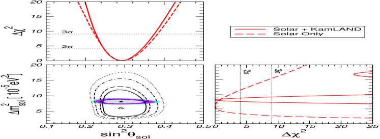
Figure 1: Regions allowed by solar and reactor data at 90%, 95%, 99%, and 3$\sigma$ C.L. for 2 d.o.f.. Unshaded regions correspond to solar data only.

2.2 Atmospheric & accelerator data

The zenith angle dependence of the $\mu$-like atmospheric neutrino data from the Super-K experiment provided the first evidence for neutrino oscillations in 1998, an effect confirmed also by other atmospheric neutrino experiments [3]. The dip in the $L/E$ distribution of the atmospheric $\nu_{\mu}$ survival probability seen in Super-K gives a clearer signature for neutrino oscillations.

The analysis summarized below includes the most recent charged-current atmospheric neutrino data from Super-K, with the $e$-like and $\mu$-like data samples of sub- and multi-GeV contained events grouped into 10 zenith-angle bins, with 5 angular bins of stopping muons and 10 through-going bins of up-going muon events. No information on $\nu_{\tau}$ appearance, multi-ring $\mu$ and neutral-current events is used since an efficient Monte-Carlo simulation of these data would require more details of the Super-K experiment, in particular of the way the neutral-current signal is extracted from the data (more details in Refs. [19, 23]). In contrast to previous analyses using the Bartol fluxes [24], here we use three–dimensional atmospheric neutrino fluxes [12]. This way one obtains the regions of two-flavour $\nu_{\mu}\to\nu_{\tau}$ oscillation parameters $\sin^{2}\theta_{\textsc{atm}}$ and $\Delta m^{2}_{\textsc{atm}}$ shown by the hollow contours in Fig. 2. Note that the $\Delta m^{2}_{\textsc{atm}}$ values obtained with the three–dimensional atmospheric neutrino fluxes are lower than obtained previously [19], in good agreement with the results of the Super-K collaboration [25].

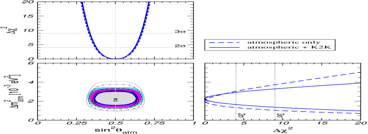
Figure 2: $\sin^{2}\theta_{\textsc{atm}}$–$\Delta m^{2}_{\textsc{atm}}$ regions allowed at 90%, 95%, 99%, and 3$\sigma$ C.L. for 2 d.o.f. (unshaded regions include atmospheric data only).

The KEK to Kamioka (K2K) long-baseline neutrino oscillation experiment [5] tests $\nu_{\mu}$ disappearance in the same $\Delta m^{2}$ region as probed by atmospheric neutrinos. The neutrino beam is produced by a 12 GeV proton beam from the KEK proton synchrotron, and has 98% muon neutrinos with 1.3 GeV mean energy. The beam is controlled by a near detector 300 m away from the proton target. Information on neutrino oscillations is obtained by comparing this near detector data with the $\nu_{\mu}$ content of the beam observed by the Super-K detector at a distance of 250 km.

The K2K-I data sample gave 56 events in Super-K, whereas $80.1^{+6.2}_{-5.4}$ were expected for no oscillations. The probability that the observed flux is explained by a statistical fluctuation without neutrino oscillations is less than 1% [5]. K2K-II started in Fall 2002, and released data at the Neutrino2004 conference [5] corresponding to $4.1\times 10^{19}$ protons on target, comparable to the K2K-I sample. Altogether K2K-I and K2K-II give 108 events in Super-K, to be compared with $150.9^{+11.6}_{-10.0}$ expected for no oscillations. Out of the 108 events 56 are so-called single-ring muon events. This data sample contains mainly muon events from the quasi-elastic scattering $\nu_{\mu}+p\to\mu+n$, and the reconstructed energy is closely related to the true neutrino energy. The K2K collaboration finds that the observed spectrum is consistent with the one expected for no oscillation only at a probability of 0.11%, whereas the spectrum predicted by the best fit oscillation parameters has a probability of 52% [5].

The re-analysis of K2K data given in [1] uses the energy spectrum of the 56 single-ring muon events from K2K-I + K2K-II (unfortunately not the full K2K data sample of 108 events, for lack of information outside the K2K collaboration). It is reasonable to fit the data divided into 15 bins in reconstructed neutrino energy. One finds that the $\Delta m^{2}$ indicated by the $\nu_{\mu}$ disappearance in K2K agrees with atmospheric neutrino results, providing the first confirmation of oscillations with $\Delta m^{2}_{\textsc{atm}}$ from a man-made neutrino source. However currently K2K gives a weak limit on the mixing angle due to low statistics.

The shaded regions in Fig. 2 are the allowed ($\sin^{2}\theta_{\textsc{atm}}$, $\Delta m^{2}_{\textsc{atm}}$) regions that follow from the combined analysis of K2K and Super-K atmospheric neutrino data. One sees that, although the determination of $\sin^{2}\theta_{\textsc{atm}}$ is completely dominated by atmospheric data, the K2K data start already to constrain the allowed region of $\Delta m^{2}_{\textsc{atm}}$. Note also that, despite the downward shift of $\Delta m^{2}_{\textsc{atm}}$ implied by the new atmospheric fluxes, the new result is statistically compatible both with the previous one in [19] and with the value obtained by the Super-K $L/E$ analysis [3]. Note that the K2K constraint on $\Delta m^{2}_{\textsc{atm}}$ from below is important for future long-baseline experiments, as such experiments are drastically affected if $\Delta m^{2}_{\textsc{atm}}$ lies in the lower part of the 3$\sigma$ range indicated by the atmospheric data alone.

3 THREE NEUTRINOS

The effective leptonic mixing matrix in various gauge theories of massive neutrinos such as seesaw models was first systematically studied in [8]. Its simplest unitary form can be taken as

$$K=\omega_{23}\omega_{13}\omega_{12}$$

where each factor contains an angle and a phase,

$$\omega_{13}=\left(\begin{array}[]{ccccc}c_{13}&0&e^{i\phi_{13}}s_{13}\\ 0&1&0\\ -e^{-i\phi_{13}}s_{13}&0&c_{13}\end{array}\right)\,.$$

This form holds exactly in radiative models of neutrino mass [26, 27] and approximately in the high-scale seesaw and models where supersymmetry is the origin of neutrino mass [28]. Deviations from unitarity may be phenomenologically important [29] in the inverse seesaw [30]. Here we stick to the form above. All three phases in $K$ are physical [31], one corresponds to the Kobayashi-Maskawa phase of the quarks (Dirac-phase) and affects neutrino oscillations, while the two Majorana phases show up in neutrinoless double beta decay and other lepton-number violating processes [31, 32]. Two of the three angles determine solar and atmospheric oscillations, $\theta_{12}\equiv\theta_{\textsc{sol}}$ and $\theta_{23}\equiv\theta_{\textsc{atm}}$.

Since current neutrino oscillation experiments are not sensitive to CP violation, we will neglect all phases (future neutrino factories aim at probing the effects of the Dirac phase [33]). In this approximation three-neutrino oscillations depend on the three mixing parameters $\sin^{2}\theta_{12},\sin^{2}\theta_{23},\sin^{2}\theta_{13}$ and on the two mass-squared differences $\Delta m^{2}_{\textsc{sol}}\equiv\Delta m^{2}_{21}\equiv m^{2}_{2}-m^{2}_{1}$ and $\Delta m^{2}_{\textsc{atm}}\equiv\Delta m^{2}_{31}\equiv m^{2}_{3}-m^{2}_{1}$ characterizing solar and atmospheric neutrinos. The hierarchy $\Delta m^{2}_{\textsc{sol}}\ll\Delta m^{2}_{\textsc{atm}}$ implies that one can set, to a good approximation, $\Delta m^{2}_{\textsc{sol}}=0$ in the analysis of atmospheric and K2K data, and $\Delta m^{2}_{\textsc{atm}}$ to infinity in the analysis of solar and KamLAND data. The relevant neutrino oscillation data in a global three-neutrino analysis are those of sections 2.1 and 2.2 together with the constraints from reactor experiments [34].

The global three–neutrino oscillation results are summarized in Fig. 3 and in Tab. 1. In the upper panels $\Delta\chi^{2}$ is shown as a function of the parameters $\sin^{2}\theta_{12},\sin^{2}\theta_{23},\sin^{2}\theta_{13},\Delta m^{2}_{21},\Delta m^{2}_{31}$, minimized with respect to the undisplayed parameters. The lower panels show two-dimensional projections of the allowed regions in the five-dimensional parameter space. The best fit values and the allowed 3$\sigma$ ranges of the oscillation parameters from the global data are summarized in Tab. 1. This table gives the current status of the three–flavour neutrino oscillation parameters.

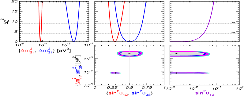
Figure 3: Three–neutrino regions allowed by the world’s oscillation data at 90%, 95%, 99%, and 3$\sigma$ C.L. for 2 d.o.f.

parameter	best fit	3$\sigma$ range
$\Delta m^{2}_{21}\>[10^{-5}~{}\mathrm{eV}^{2}]$	7.900	7.1–8.9
$\Delta m^{2}_{31}\>[10^{-3}~{}\mathrm{eV}^{2}]$	2.200	1.4–3.3
$\sin^{2}\theta_{12}$	0.300	0.23–0.38
$\sin^{2}\theta_{23}$	0.500	0.34–0.68
$\sin^{2}\theta_{13}$	0.000	$\leq$ 0.051

Table 1: Three–neutrino oscillation parameters from [1].

In a three–neutrino scheme CP violation disappears when two neutrinos become degenerate [8] or when one angle vanishes, $\theta_{13}\to 0$. Genuine three–flavour effects are associated to the mass hierarchy parameter $\alpha\equiv\Delta m^{2}_{\textsc{sol}}/\Delta m^{2}_{\textsc{atm}}$ and the mixing angle $\theta_{13}$.

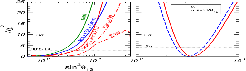
Figure 4: Determination of $\alpha\equiv\Delta m^{2}_{\textsc{sol}}/\Delta m^{2}_{\textsc{atm}}$ and bound on $\sin^{2}\theta_{13}$ from current data.

The left panel in Fig. 4 gives the parameter $\alpha$ as determined from the global $\chi^{2}$ analysis of [1]. The figure also gives $\Delta\chi^{2}$ as a function of the parameter combination $\alpha\sin 2\theta_{12}$ which, to leading order, determines the long baseline $\nu_{e}\to\nu_{\mu}$ oscillation probability [35, 36]. The last unknown angle in the three–neutrino leptonic mixing matrix is $\theta_{13}$, for which only an upper bound exists. The left panel in Fig. 4 gives $\Delta\chi^{2}$ as a function of $\sin^{2}\theta_{13}$ for different data sample choices. One finds that the new data from KamLAND have a surprisingly strong impact on this bound. Before the KamLAND-2004 data the bound on $\sin^{2}\theta_{13}$ from global data was dominated by the CHOOZ reactor experiment, together with the determination of $\Delta m^{2}_{31}$ from atmospheric data. However, with the KamLAND-2004 data the bound becomes comparable to the reactor bound, and contributes significantly to the final global bound 0.022 (0.047) at 90% C.L. (3$\sigma$) for 1 d.o.f. This improved $\sin^{2}\theta_{13}$ bound follows from the strong spectral distortion found in the 2004 sample [1].

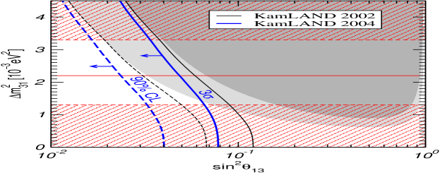
Figure 5: Upper bound on $\sin^{2}\theta_{13}$ (1 d.o.f.) from solar+reactor data versus $\Delta m^{2}_{\textsc{atm}}$. Dashed (solid) curves correspond to 90% (3$\sigma$) C.L. bounds, thick ones include KamLAND-2004 data, thin ones do not. Light (dark) regions are excluded by CHOOZ at 90% (3$\sigma$) C.L. The current $\Delta m^{2}_{\textsc{atm}}$ best fit value is indicated by the horizontal line, hatched regions are excluded by atmospheric + K2K data at 3$\sigma$.

Note that, since the reactor bound on $\sin^{2}\theta_{13}$ quickly deteriorates as $\Delta m^{2}_{\textsc{atm}}$ decreases (see Fig. 5), the improvement is especially important at low $\Delta m^{2}_{\textsc{atm}}$ values, as implied by the new three–dimensional atmospheric fluxes [12]. In Fig. 5 we show the upper bound on $\sin^{2}\theta_{13}$ as a function of $\Delta m^{2}_{\textsc{atm}}$ from CHOOZ data alone compared to the bound from an analysis including solar and reactor neutrino data. One finds that, although for larger $\Delta m^{2}_{\textsc{atm}}$ values the bound on $\sin^{2}\theta_{13}$ is dominated by CHOOZ, for $\Delta m^{2}_{\textsc{atm}}\raise 1.29167pt\hbox{$\;<$\kern-7.5pt\raise-4.73611pt\hbox{$\sim\;$}}2\times 10^{-3}\mathrm{eV}^{2}$ the solar + KamLAND data start being relevant. The bounds implied by the 2002 and 2004 KamLAND data are compared in Fig. 5. In addition to reactor and accelerator neutrino oscillation searches, future studies of the day/night effect in large water Cerenkov solar neutrino experiments like UNO or Hyper-K [37] may give valuable information on $\sin^{2}\theta_{13}$ [38].

4 WHAT ELSE

Neutrino oscillation data are sensitive only to mass differences, not to the absolute neutrino masses. Nor do they have any bearing on the fundamental issue of whether neutrinos are Dirac or Majorana particles [31, 32]. The significance of the $\beta\beta_{0\nu}$ decay is given by the fact that, in a gauge theory, irrespective of the mechanism that induces $\beta\beta_{0\nu}$ , it must also produce a Majorana neutrino mass [39], as illustrated in Fig. 6.

Figure 6: Equivalence between $\beta\beta_{0\nu}$ and Majorana mass in gauge theories [39].

Although quantitative implications of this “black-box” argument are model-dependent, any “natural” gauge theory obeys the theorem.

Now that oscillations have been confirmed we know that $\beta\beta_{0\nu}$ must be induced by the exchange of light Majorana neutrinos. The corresponding amplitude is sensitive both to the absolute scale of neutrino mass as well as the two Majorana CP phases in the minimal 3-neutrino mixing matrix [8].

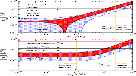
Figure 7: Neutrino-mass-induced $\beta\beta_{0\nu}$ from current oscillation data versus current and projected experimental sensitivities.

Fig. 7 shows the estimated average mass parameter characterizing the neutrino exchange contribution to $\beta\beta_{0\nu}$ versus the lightest neutrino mass. The upper (lower) panel corresponds to the cases of normal (inverted) neutrino mass spectra. The calculation takes into account the current neutrino oscillation parameters from [1] and the nuclear matrix elements of [16]. In contrast to the normal hierarchy, where a destructive interference of neutrino amplitudes is possible, the inverted neutrino mass hierarchy implies a “lower” bound for the $\beta\beta_{0\nu}$ amplitude. Quasi-degenerate neutrinos [40] such as predicted in [17], give the largest $\beta\beta_{0\nu}$ amplitude, as can be seen by the rising diagonal bands on the right-hand side of the panels. Future experiments [41] will provide an independent confirmation of the present hint [42] and push the sensitivity to inverse hierarchy models. Complementary information on the absolute scale of neutrino mass comes from beta decays searches [43] as well as cosmology [44].

In conclusion, we can say that, despite the great progress achieved recently we are still very far from a “road map” to the ultimate theory of neutrino properties. We have no idea of the underlying neutrino mass generation mechanism, its characteristic scale or its flavor structure. We have still a long way to go and need more data, especially a confirmation of the LSND and neutrinoless double beta decay hints.

References

- [1] M. Maltoni, T. Schwetz, M. A. Tortola and J. W. F. Valle, New J. Phys. 6 (2004) 122 [hep-ph 0405172] and references therein.
- [2] M. Chen, these proceedings.
- [3] T. Kajita, these proceedings.
- [4] K. Inoue, these proceedings.
- [5] M. Shaevitz, these proceedings.
- [6] S. Weinberg, Phys. Rev. D22 1694 (1980).
- [7] P. Minkowski, Phys. Lett. B 67 (1977) 421; T. Yanagida, KEK lectures, 1979; M. Gell-Mann, P. Ramond, R. Slansky, CERN Print-80-0576; R. Mohapatra, G. Senjanovic, Phys. Rev. D 23 (1981) 16; for the general description of the seesaw see Ref. [8]
- [8] J. Schechter and J. W. F. Valle, Phys. Rev. D22, 2227 (1980); D25, 774 (1982).
- [9] M. Fukugita and T. Yanagida, Phys. Lett. B 174 (1986) 45.
- [10] M. Goodman, Neutrino Oscillation Industry Web-Page, http://neutrinooscillation.org/.
- [11] J. N. Bahcall and M. H. Pinsonneault, Phys. Rev. Lett. 93, 121301 (2004)
- [12] M. Honda, T. Kajita, K. Kasahara and S. Midorikawa, astro-ph/0404457.
- [13] S. P. Mikheev and A. Y. Smirnov, Sov. J. Nucl. Phys. 42, 913 (1985).
- [14] L. Wolfenstein, Phys. Rev. D17, 2369 (1978).
- [15] L. Wolfenstein, Phys. Lett. B 107 77 (1981); J. Schechter and J. W. F. Valle, Phys. Rev. D24, 1883 (1981), Err. D25, 283 (1982); see also AIP Conf. Proc. 687, 16 (2003)
- [16] S. M. Bilenky, A. Faessler and F. Simkovic, Phys. Rev. D70 033003 (2004)
- [17] K. Babu, E. Ma and J. W. F. Valle, Phys. Lett. B552 207 (2003); M. Hirsch et al, Phys. Rev. D 69 093006 (2004)
- [18] C. Albright, hep-ph/0407155; W. Grimus et al, hep-ph/0408123; S. Barr, I. Dorsner, Nucl. Phys. B 585 79 (2000); H. S. Goh et al, Phys. Lett. B 587 105 (2004); M. Raidal, hep-ph/0404046; H. Minakata, A. Smirnov, hep-ph/0405088; J. Ferrandis, S. Pakvasa, Phys. Lett. B 603, 184 (2004); G. Altarelli, F. Feruglio, New J. Phys. 6 (2004) 106
- [19] M. Maltoni et al, Phys. Rev. D68, 113010 (2003); Phys. Rev. D67, 013011 (2003)
- [20] G. Fogli et al, Phys. Rev. D66, 053010 (2002)
- [21] A. B. Balantekin and H. Yuksel, Phys. Rev. D68, 113002 (2003)
- [22] G. Fiorentini et al, Phys. Lett. B558, 15 (2003); H. Nunokawa, W. C. Teves and R. Zukanovich, JHEP 11, 020 (2003)
- [23] M. Gonzalez-Garcia et al, Phys. Rev. D63, 033005 (2001)
- [24] G. Barr, T. K. Gaisser and T. Stanev, Phys. Rev. D39, 3532 (1989).
- [25] http://eps2003.physik.rwth-aachen.de.
- [26] A. Zee, Phys. Lett. B93, 389 (1980).
- [27] K. S. Babu, Phys. Lett. B203, 132 (1988).
- [28] M. Hirsch and J. W. F. Valle, New J. Phys. 6, 76 (2004) [hep-ph/0405015]
- [29] J. Bernabeu et al, Phys. Lett. B187, 303 (1987); G. Branco, M. Rebelo, J. W. F. Valle, Phys. Lett. B225, 385 (1989); N. Rius, J. W. F. Valle, Phys. Lett. B246, 249 (1990); F. Deppisch, J. W. F. Valle, hep-ph/0406040.
- [30] R. N. Mohapatra and J. W. F. Valle, Phys. Rev. D34, 1642 (1986).
- [31] J. Schechter and J. W. F. Valle, Phys. Rev. D23, 1666 (1981).
- [32] M. Doi et al, Phys. Lett. B102, 323 (1981); S. Bilenky et al, Phys. Lett. B 94 49 (1980)
- [33] K. Dick, M. Freund, M. Lindner and A. Romanino, Nucl. Phys. B562, 29 (1999)
- [34] M. Apollonio et al, Phys. Lett. B466, 415 (1999); F. Boehm et al, Phys. Rev. D64, 112001 (2001)
- [35] M. Freund, Phys. Rev. D64, 053003 (2001)
- [36] E. K. Akhmedov et al, hep-ph/0402175.
- [37] C. Yanagisawa, Proc. of AHEP2003, published at JHEP, PRHEP-AHEP2003/062, accessible from http://ific.uv.es/ahep/.
- [38] E. K. Akhmedov et al, JHEP 0405 057 (2004); M. Blennow et al, Phys. Rev. D69, 073006 (2004)
- [39] J. Schechter and J. W. F. Valle, Phys. Rev. D25, 2951 (1982)
- [40] D. Caldwell, R. Mohapatra, Phys. Rev. D48, 3259 (1993); A. Ioannisian and J. W. F. Valle, Phys. Lett. B 332 93 (1994); A. S. Joshipura, Z. Phys. C 64 (1994) 31; S. Antusch and S. F. King, Nucl. Phys. B 705 (2005) 239
- [41] H. V. Klapdor et al, hep-ph/9910205.
- [42] H. Klapdor etal, Phys. Lett. B 586 (2004) 198
- [43] A. Osipowicz, et al, hep-ex/0109033.
- [44] S. Pastor, hep-ph/0306233; S. Hannestad, hep-ph/0404239; G. Fogli et al, hep-ph/0408045