LPSC 05–63

hep-ph/0508068

Transverse-momentum resummation and
the spectrum of the Higgs boson at the LHC

Giuseppe Bozzi^(a), Stefano Catani^(b),
Daniel de Florian^(c) and Massimiliano Grazzini^(b)

^(a)Laboratoire de Physique Subatomique et de Cosmologie,

Université Joseph Fourier/CNRS–IN2P3, F-38026 Grenoble, France

^(b)INFN, Sezione di Firenze and Dipartimento di Fisica, Università di Firenze,

I-50019 Sesto Fiorentino, Florence, Italy

^(c)Departamento de Física, FCEYN, Universidad de Buenos Aires,

(1428) Pabellón 1 Ciudad Universitaria, Capital Federal, Argentina

Abstract

We consider the transverse-momentum ($q_{T}$) distribution of generic high-mass systems (lepton pairs, vector bosons, Higgs particles, ….) produced in hadron collisions. At small $q_{T}$, we concentrate on the all-order resummation of the logarithmically-enhanced contributions in QCD perturbation theory. We elaborate on the $b$-space resummation formalism and introduce some novel features: the large logarithmic contributions are systematically exponentiated in a process-independent form and, after integration over $q_{T}$, they are constrained by perturbative unitarity to give a vanishing contribution to the total cross section. At intermediate and large $q_{T}$, resummation is consistently combined with fixed-order perturbative results, to obtain predictions with uniform theoretical accuracy over the entire range of transverse momenta. The formalism is applied to Standard Model Higgs boson production at LHC energies. We combine the most advanced perturbative information available at present for this process: resummation up to next-to-next-to-leading logarithmic accuracy and fixed-order perturbation theory up to next-to-leading order. The results show a high stability with respect to perturbative QCD uncertainties.

LPSC 05–63

August 2005

1 Introduction

This paper is devoted to study the transverse-momentum ($q_{T}$) spectrum of high-mass systems produced by hard-scattering of partons in hadron–hadron collisions. In Ref. [1] we presented some quantitative results on the $q_{T}$ spectrum of the Standard Model (SM) Higgs boson, produced via the gluon fusion mechanism, at LHC energies. The formalism used in Ref. [1] is quite general and applies to the transverse-momentum distribution of generic high-mass systems (lepton pairs, vector bosons, Higgs particles, ..) produced in hadron collisions. The purpose of the present paper is twofold. Owing to its general applicability, we find it useful to first describe and discuss the formalism with quite some details. We then perform a more systematic phenomenological analysis of the $q_{T}$ distribution of the Higgs boson at the LHC.

In this introductory section, rather than illustrating the resummation formalism in general terms, we mainly consider the explicit case of the $q_{T}$ spectrum of the Higgs boson. This also serves for underlying some general features of the formalism in concrete, rather than abstract, terms.

Within the SM of electroweak interactions, the Higgs boson [2] is responsible for the mechanism of the electroweak symmetry breaking, but this particle has so far eluded experimental discovery. Direct searches at LEP have established a lower bound of $114.4$ GeV [3] on the mass $M_{H}$ of the SM Higgs boson, whereas SM fits of electroweak precision data lead to the upper limit $M_{H}<260$ GeV at $95\%$ CL [4]. The next search for Higgs boson(s) will be carried out at hadron colliders, namely, the Fermilab Tevatron [5, 6] and the CERN LHC [7, 8].

The main production mechanism of the SM Higgs boson $H$ at hadron colliders is the gluon fusion process $gg\rightarrow H$, through a heavy-quark (mainly, top-quark) loop. When combined with the decay channels $H\rightarrow\gamma\gamma$, $H\rightarrow WW$ and $H\rightarrow ZZ$, this production mechanism is one of the most important for Higgs boson searches and studies over the entire mass range, 100 GeV$\raisebox{-2.58334pt}{\hbox to0.0pt{$\,\sim\,$\hss}}\raisebox{1.72218pt}{$\,<\,$}M_{H}\raisebox{-2.58334pt}{\hbox to0.0pt{$\,\sim\,$\hss}}\raisebox{1.72218pt}{$\,<\,$}$1 TeV, to be investigated at the LHC [7]. To fully exploit the physics potential of the gluon fusion process, it is relevant to provide reliable theoretical predictions for the corresponding total cross section and for the associated distributions, such as, for instance, the Higgs $q_{T}$ distribution. The dominant source of theoretical uncertainties on these quantities is the effect of QCD radiative corrections, which, therefore, have to be carefully investigated.

The total cross section for Higgs boson production by gluon fusion has been computed in QCD perturbation theory at the leading order (LO), ${\cal O}(\alpha_{\mathrm{S}}^{2})$, at the next-to-leading order (NLO) [9, 10] and at the next-to-next-to-leading order (NNLO) [11–14] in the QCD coupling $\alpha_{\mathrm{S}}$. The NNLO computation of the rapidity distribution of the Higgs boson has recently been completed [15]. A key point of this theoretical activity is that the origin of the dominant perturbative contributions to the total cross section has been identified and understood: the bulk of the radiative corrections is due to virtual and soft-gluon terms [12]. This point has a twofold relevance. On one side, it explains the observation [16] of the validity of the large-$M_{t}$ approximation ($M_{t}$ being the mass of the top quark) in the calculation at the NLO, and, therefore, it justifies the use of the same approximation at and beyond the NNLO. On the other side, it allows to estimate higher-order QCD contributions by supplementing the NNLO calculation with an all-order resummation of the logarithmically-enhanced terms due to multiple soft-gluon emission [17]. Having these terms under control allows us to reliably predict the value of the cross section and, more importantly, to reduce the associated perturbative uncertainty at the level of about $\pm 10\%$ [17].

When studying the $q_{T}$ distribution of the Higgs boson in QCD perturbation theory, it is convenient to start by considering separately the large-$q_{T}$ and small-$q_{T}$ regions.

The large-$q_{T}$ region is identified by the condition $q_{T}\sim M_{H}$. In this region, the perturbative series is controlled by a small expansion parameter, $\alpha_{\mathrm{S}}(M_{H}^{2})$, and calculations based on the truncation of the series at a fixed order in $\alpha_{\mathrm{S}}$ are theoretically justified. SM Higgs boson production at large $q_{T}$ via gluon fusion has to be accompanied by the radiation of at least one recoiling parton, so the LO term for this observable is of ${\cal O}(\alpha_{\mathrm{S}}^{3})$. The LO calculation was reported in Ref. [18]; it shows that the large-$M_{t}$ approximation works well as long as $M_{H}\raisebox{-2.58334pt}{\hbox to0.0pt{$\,\sim\,$\hss}}\raisebox{1.72218pt}{$\,<\,$}2M_{t}$ and $q_{T}\raisebox{-2.58334pt}{\hbox to0.0pt{$\,\sim\,$\hss}}\raisebox{1.72218pt}{$\,<\,$}M_{t}$. Similar results on the validity of the large-$M_{t}$ approximation were obtained in the case of the associated production of a Higgs boson plus 2 jets (2 recoiling partons at large transverse momenta) [19]. In the framework of the large-$M_{t}$ approximation, the NLO QCD corrections to the transverse-momentum distribution of the SM Higgs boson were computed in Refs. [20–23]. Corrections to the large-$M_{t}$ approximation are considered in Ref. [24]. The numerical programs of Refs. [20, 23] can also be used to evaluate arbitrary infrared- and collinear-safe observables up to NLO in the large-$q_{T}$ region and, in the case of Ref. [23], up to NNLO when $q_{T}=0$.

In the small-$q_{T}$ region ($q_{T}\ll M_{H}$), where the bulk of events is produced, the convergence of the fixed-order expansion is spoiled, since the coefficients of the perturbative series in $\alpha_{\mathrm{S}}(M_{H}^{2})$ are enhanced by powers of large logarithmic terms, $\ln^{m}(M_{H}^{2}/q_{T}^{2})$. To obtain reliable perturbative predictions, these terms have to be resummed to all orders in $\alpha_{\mathrm{S}}$. The method to systematically perform all-order resummation of classes of logarithmically-enhanced terms at small $q_{T}$ is known [25–33]. In the case of the SM Higgs boson, resummation has been explicitly worked out at leading logarithmic (LL), next-to-leading logarithmic (NLL) [34, 35] and next-to-next-to-leading logarithmic (NNLL) [36] level.

The fixed-order and resummed approaches at small and large values of $q_{T}$ can then be matched at intermediate values of $q_{T}$, to obtain QCD predictions for the entire range of transverse momenta. Phenomenological studies of the SM Higgs boson $q_{T}$ distribution have been performed in Refs. [37, 35, 38–42, 1, 43–46], by combining resummed and fixed-order perturbation theory at different levels of theoretical accuracy. A comparison of theoretical calculations [1, 40, 42, 44] and of results from parton shower Monte Carlo generators [47–50] is presented in Ref. [51].

In the present paper we compute the Higgs boson $q_{T}$ distribution at the LHC by combining the most advanced perturbative information that is available at present: NNLL resummation at small $q_{T}$ and NLO perturbation theory at large $q_{T}$. The first results of our calculation were presented in Refs. [1, 52]. Here we perform a more complete phenomenological study and present a discussion of theoretical uncertainties.

The formalism used to obtain these results was briefly described in Refs. [33, 1] and is illustrated in detail in the present paper. Three distinctive features are anticipated here. The resummation is performed at the level of the partonic cross section; this implies that the parton distributions are evaluated at the factorization scale $\mu_{F}$, which has to be chosen of the order of the hard scale $M$. The resummed terms are embodied in a form factor that is universal: it depends only on the flavour of the partons that initiate the hard-scattering subprocess at the Born level (e.g. $q{\bar{q}}$ annihilation in the case of Drell–Yan lepton pair production, and $gg$ fusion in the case of Higgs boson production). A constraint of perturbative unitarity is imposed on the resummed terms, to the purpose of reducing the effect of unjustified higher-order contributions at large values of $q_{T}$ and, especially, at intermediate values of $q_{T}$. The constraint implies that the total cross section at the nominal fixed-order accuracy (NLO or NNLO) is recovered upon integration over $q_{T}$ of the transverse-momentum spectrum (at NLL+LO or NNLL+NLO).

The paper is organized as follows. In Sect. 2 the resummation formalism is discussed in detail. After illustrating the general aspects of our approach in Sect. 2.1, we discuss the structure of the resummed cross section in Sect. 2.2. The relation to the standard $b$-space resummation is given in Sect. 2.3. Sect. 2.4 is devoted to the finite component of the cross section. In Sect. 3 we apply the resummation formalism to the production of the SM Higgs boson at the LHC. In Sect. 4 we draw our conclusions. In Appendix A we discuss the details of the exponentiation in the general multiflavour case. In Appendix B we illustrate the calculation of the Bessel integrals required in the computation of the perturbative expansion of the resummed cross section.

2 Transverse-momentum resummation

The formalism [1, 33] that we use to compute the $q_{T}$ distribution of the Higgs boson applies to more general hard-scattering processes. Therefore, we describe it in general terms.

2.1 The resummation formalism: from small to large values of $q_{T}$

We consider the inclusive hard-scattering process

$$h_{1}(p_{1})+h_{2}(p_{2})\rightarrow F(M,q_{T})+X\;\;,$$ (1)

where the collision of the two hadrons $h_{1}$ and $h_{2}$ with momenta $p_{1}$ and $p_{2}$ produces the triggered final-state system $F$, accompanied by an arbitrary and undetected final state $X$. We denote by $\sqrt{s}$ the centre-of-mass energy of the colliding hadrons $(s=(p_{1}+p_{2})^{2}\simeq 2p_{1}p_{2})$. The observed final state $F$ is a generic system of non-QCD partons such as one or more vector bosons $(\gamma^{*},W,Z,\dots)$, Higgs particles, Drell–Yan (DY) lepton pairs and so forth. We do not consider the production of strongly interacting particles (hadrons, jets, heavy quarks, …), since in this case the resummation formalism of small-$q_{T}$ logarithms has not yet been fully developed.

Throughout the paper we limit ourselves to considering the case in which only the total invariant mass $M$ and transverse momentum $q_{T}$ of the system $F$ are measured. According to the QCD factorization theorem (see Ref. [53] and references therein), the corresponding transverse-momentum differential cross section $d{\hat{\sigma}}_{F}/dq_{T}^{2}$ can be written as

$$\frac{d\sigma_{F}}{dq_{T}^{2}}(q_{T},M,s)=\sum_{a,b}\int_{0}^{1}dx_{1}\,\int_{0}^{1}dx_{2}\,f_{a/h_{1}}(x_{1},\mu_{F}^{2})\,f_{b/h_{2}}(x_{2},\mu_{F}^{2})\;\frac{d{\hat{\sigma}}_{F\,ab}}{dq_{T}^{2}}(q_{T},M,{\hat{s}};\alpha_{\mathrm{S}}(\mu_{R}^{2}),\mu_{R}^{2},\mu_{F}^{2})\;,$$ (2)

where $f_{a/h}(x,\mu_{F}^{2})$ ($a=q_{f},{\bar{q}_{f}},g$) are the parton densities of the colliding hadrons at the factorization scale $\mu_{F}$, $d{\hat{\sigma}}_{F\,ab}/dq_{T}^{2}$ are the partonic cross sections, ${\hat{s}}=x_{1}x_{2}s$ is the partonic centre-of-mass energy, and $\mu_{R}$ is the renormalization scale. Throughout the paper we use parton densities as defined in the ${\overline{\rm MS}}$ factorization scheme, and $\alpha_{\mathrm{S}}(q^{2})$ is the QCD running coupling in the ${\overline{\rm MS}}$ renormalization scheme.

The partonic cross section is computable in QCD perturbation theory as a power series expansion in $\alpha_{\mathrm{S}}$. We assume that at the parton level the system $F$ is produced with vanishing $q_{T}$ (i.e. with no accompanying final-state radiation) in the lowest-order approximation, so that the corresponding cross section is $d{\hat{\sigma}}^{(0)}_{F\,c{\bar{c}}}/dq_{T}^{2}\propto\delta(q_{T}^{2})$. Since $F$ is colourless, the lowest-order partonic subprocess, $c+{\bar{c}}\rightarrow F$, is either $q{\bar{q}}$ annihilation ($c=q$), as in the case of $\gamma^{*},W$ and $Z$ production, or $gg$ fusion ($c=g$), as in the case of the production of the SM Higgs boson $H$.

As recalled in Sect. 1, higher-order perturbative contributions to the partonic cross section $d{\hat{\sigma}}_{F\,ab}/dq_{T}^{2}$ contain logarithmic terms of the type $\ln^{m}(M^{2}/q_{T}^{2})$ that become large in the small-$q_{T}$ region ($q_{T}\ll M$). Therefore, we introduce the following decomposition of the partonic cross section in Eq. (2):

$$\frac{d{\hat{\sigma}}_{F\,ab}}{dq_{T}^{2}}=\frac{d{\hat{\sigma}}_{F\,ab}^{(\rm res.)}}{dq_{T}^{2}}+\frac{d{\hat{\sigma}}_{F\,ab}^{(\rm fin.)}}{dq_{T}^{2}}\,.$$ (3)

The distinction between the two terms on the right-hand side is purely theoretical. The first term, $d{\hat{\sigma}}_{F\,ab}^{(\rm res.)}$, on the right-hand side contains all the logarithmically-enhanced contributions, $(\alpha_{\mathrm{S}}^{n}/q_{T}^{2})\,\ln^{m}(M^{2}/q_{T}^{2})$, at small $q_{T}$, and has to be evaluated by resumming them to all orders in $\alpha_{\mathrm{S}}$. The second term, $d{\hat{\sigma}}_{F\,ab}^{(\rm fin.)}$, is free of such contributions, and can be computed by fixed-order truncation of the perturbative series. More precisely, we define the ‘finite’ component $d{\hat{\sigma}}_{F\,ab}^{(\rm fin.)}$ in such a way that we have

$$\lim_{Q_{T}\rightarrow 0}\;\int_{0}^{Q_{T}^{2}}dq_{T}^{2}\;\Bigl{[}\frac{d{\hat{\sigma}}_{F\,ab}^{(\rm fin.)}}{dq_{T}^{2}}\Bigr{]}_{\rm f.o.}=0\;,$$ (4)

where the right-hand side vanishes order-by-order in perturbation theory. In particular, this implies that any perturbative contributions proportional to $\delta(q_{T}^{2})$ have been removed from $d{\hat{\sigma}}_{F\,ab}^{(\rm fin.)}$ and included in $d{\hat{\sigma}}_{F\,ab}^{(\rm res.)}$.

The ‘resummed’ component $d{\hat{\sigma}}_{F\,ab}^{(\rm res.)}$ of the partonic cross section cannot, of course, be evaluated by computing all the logarithmic contributions in the perturbative series. However, as discussed in Sect. 2.2, these contributions can systematically be organized in classes of LL, NLL, $\dots$ terms and, then, this logarithmic expansion can be truncated at a given logarithmic accuracy.

In summary, the $q_{T}$ distribution in Eq. (2) is evaluated, in practice, by replacing the partonic cross section on the right-hand side as follows

$$\frac{d{\hat{\sigma}}_{F\,ab}}{dq_{T}^{2}}\;\longrightarrow\;\Bigl{[}\frac{d{\hat{\sigma}}_{F\,ab}^{(\rm res.)}}{dq_{T}^{2}}\Bigr{]}_{\rm l.a.}+\;\Bigl{[}\frac{d{\hat{\sigma}}_{F\,ab}^{(\rm fin.)}}{dq_{T}^{2}}\Bigr{]}_{\rm f.o.}\,.$$ (5)

The first and second terms on the right-hand side denote the truncation of the resummed and finite components at a given logarithmic accuracy and at a given fixed order, respectively. The resummed component gives the dominant contribution in the small-$q_{T}$ region, while the finite component dominates at large values of $q_{T}$. The two components have to be consistently matched at intermediate values of $q_{T}$, so as to obtain a theoretical prediction with uniform formal accuracy over the entire range of $q_{T}$, from $q_{T}\ll M$ up to $q_{T}\sim M$. To this aim, we compute $\bigl{[}d{\hat{\sigma}}_{ab}^{(\rm fin.)}\bigr{]}_{\rm f.o.}$ starting from $\bigl{[}d{\hat{\sigma}}_{ab}\bigr{]}_{\rm f.o.}$, the usual perturbative series for the partonic cross section truncated at a given fixed order in $\alpha_{\mathrm{S}}$, and subtracting from it the perturbative truncation of the resummed component at the same fixed order in $\alpha_{\mathrm{S}}$:

$$\Bigl{[}\frac{d{\hat{\sigma}}_{F\,ab}^{(\rm fin.)}}{dq_{T}^{2}}\Bigr{]}_{\rm f.o.}=\Bigl{[}\frac{d{\hat{\sigma}}_{F\,ab}}{dq_{T}^{2}}\Bigr{]}_{\rm f.o.}-\Bigl{[}\frac{d{\hat{\sigma}}_{F\,ab}^{(\rm res.)}}{dq_{T}^{2}}\Bigr{]}_{\rm f.o.}\;.$$ (6)

Moreover, we impose the condition:

$$\left[\Bigl{[}\frac{d{\hat{\sigma}}_{F\,ab}^{(\rm res.)}}{dq_{T}^{2}}\Bigr{]}_{\rm l.a.}\right]_{\rm f.o.}=\;\Bigl{[}\frac{d{\hat{\sigma}}_{F\,ab}^{(\rm res.)}}{dq_{T}^{2}}\Bigr{]}_{\rm f.o.}\,.$$ (7)

This matching procedure guarantees that the replacement in Eq. (5) retains the full information of the perturbative calculation up to the specified fixed order plus resummation of logarithmically-enhanced contributions from higher orders. Equations (6) and (7) indeed imply that the matching is perturbatively exact, in the sense that the fixed-order truncation of the right-hand side of Eq. (5) exactly reproduces the customary fixed-order truncation of the partonic cross section in Eq. (2). The (small-$q_{T}$) resummed and (large-$q_{T}$) fixed-order approaches are thus consistently combined without double-counting (or neglecting) of perturbative contributions and by avoiding the introduction of ad-hoc boundaries (such as, for instance, the choice of some intermediate value of $q_{T}$ as ‘switching’ point between the resummed and fixed-order calculations) between the large-$q_{T}$ and small-$q_{T}$ regions.

The resummed contributions that are present in the term $\bigl{[}d{\hat{\sigma}}_{F\,ab}^{(\rm res.)}\bigr{]}_{\rm l.a.}$ of Eq. (5) are necessary and fully justified at small $q_{T}$. Nonetheless they can lead to sizeable higher-order perturbative effects also at large $q_{T}$, where the small-$q_{T}$ logarithmic approximation is not valid. To reduce the impact of these unjustified higher-order terms, we require that they give no contributions to the most basic quantity, namely the total cross section, that is not affected by small-$q_{T}$ logarithmic terms. We thus impose that the integral over $q_{T}$ of Eq. (5) exactly reproduces the fixed-order calculation of the total cross section. Since $d{\hat{\sigma}}_{F\,ab}^{(\rm fin.)}$ is evaluated in fixed-order perturbation theory, the perturbative constraint on the total cross section is achieved by imposing the following condition:

$$\int_{0}^{\infty}dq_{T}^{2}\;\Bigl{[}\frac{d{\hat{\sigma}}_{F\,ab}^{(\rm res.)}}{dq_{T}^{2}}\Bigr{]}_{\rm l.a.}=\int_{0}^{\infty}dq_{T}^{2}\;\Bigl{[}\frac{d{\hat{\sigma}}_{F\,ab}^{(\rm res.)}}{dq_{T}^{2}}\Bigr{]}_{\rm f.o.}\;.$$ (8)

Equation (8) can be regarded, in some sense, as a unitarity constraint. As a matter of fact, the logarithmic contributions that are resummed in $d{\hat{\sigma}}_{F\,ab}^{(\rm res.)}$ are, precisely speaking, plus distributions of the type $\left[(\alpha_{\mathrm{S}}^{n}/q_{T}^{2})\,\ln^{m}(M^{2}/q_{T}^{2})\right]_{+}$. Therefore, it is quite natural to require that these resummed terms give a vanishing contribution to the total cross section. Note that the bulk of the $q_{T}$ distribution is in the region $q_{T}\raisebox{-2.58334pt}{\hbox to0.0pt{$\,\sim\,$\hss}}\raisebox{1.72218pt}{$\,<\,$}M_{H}$. Since resummed and fixed-order perturbation theory controls the small-$q_{T}$ and large-$q_{T}$ regions respectively, the total cross section constraint mainly acts on the size of the higher-order contributions introduced in the intermediate-$q_{T}$ region by the matching procedure.

Another distinctive feature of the formalism illustrated so far is that we implement perturbative QCD resummation at the level of the partonic cross section. In the factorization formula (2), the parton densities are thus evaluated at the factorization scale $\mu_{F}$, as in the customary perturbative calculations at large $q_{T}$. Although we are dealing with a process characterized by two distinct hard scales, $q_{T}$ and $M$, the dominant effects from the scale region $q_{T}\ll M$ are explicitly taken into account through all-order resummation. Therefore, the central value of $\mu_{F}$ and $\mu_{R}$ has to be set equal to $M_{H}$, the ‘remaining’ typical hard scale of the process. Then the theoretical accuracy of the resummed calculation can be investigated as in customary fixed-order calculations, by varying $\mu_{F}$ and $\mu_{R}$ around this central value.

At small values of $q_{T}$, the perturbative QCD approach has to be supplemented with non-perturbative contributions, since they become relevant as $q_{T}$ decreases. A discussion on non-perturbative effects on the $q_{T}$ distribution of the SM Higgs boson is presented in Sect. 3.1.

The resummation and matching formalism, which we have so far illustrated in quite general terms, is set up to deal with the transverse-momentum region where $q_{T}\raisebox{-2.58334pt}{\hbox to0.0pt{$\,\sim\,$\hss}}\raisebox{1.72218pt}{$\,<\,$}M$. Resummation of small-$q_{T}$ logarithms cannot lead to any theoretical improvements in the large-$q_{T}$ region, where those logarithms are not the dominant contributions. When $q_{T}\raisebox{-2.58334pt}{\hbox to0.0pt{$\,\sim\,$\hss}}\raisebox{1.72218pt}{$\,>\,$}M$, the use of the resummation formalism is no longer justified (recommended), and we have to use the customary fixed-order perturbative expansion.

2.2 The resummed component

The method to systematically resum the logarithmically-enhanced contributions at small $q_{T}$ was set up [26–30] shortly after the first resummed calculation of the DY $q_{T}$ spectrum to double logarithmic accuracy [25]. The resummation procedure has to be carried out in the impact-parameter space, to correctly take into account the kinematics constraint of transverse-momentum conservation. The resummed component of the transverse-momentum cross section in Eq. (3) is then obtained by performing the inverse Fourier (Bessel) transformation with respect to the impact parameter $b$. We write

$$\!\!\!\frac{d{\hat{\sigma}}_{F\,ab}^{(\rm res.)}}{dq_{T}^{2}}(q_{T},M,{\hat{s}};\alpha_{\mathrm{S}}(\mu_{R}^{2}),\mu_{R}^{2},\mu_{F}^{2}) = \frac{M^{2}}{\hat{s}}\;\int\frac{d^{2}{\bf b}}{4\pi}\;e^{i{\bf b}\cdot q_{T}}\;{\cal W}_{ab}^{F}(b,M,{\hat{s}};\alpha_{\mathrm{S}}(\mu_{R}^{2}),\mu_{R}^{2},\mu_{F}^{2})$$ (9)

$$= \frac{M^{2}}{\hat{s}}\;\int_{0}^{\infty}db\;\frac{b}{2}\;J_{0}(bq_{T})\;{\cal W}_{ab}^{F}(b,M,{\hat{s}};\alpha_{\mathrm{S}}(\mu_{R}^{2}),\mu_{R}^{2},\mu_{F}^{2})\;,$$ (10)

where $J_{0}(x)$ is the 0th-order Bessel function.

The perturbative and process-dependent factor ${\cal W}_{ab}^{F}$ embodies the all-order dependence on the large logarithms $\ln M^{2}b^{2}$ at large $b$, which correspond to the $q_{T}$-space terms $\ln M^{2}/q_{T}^{2}$ that are logarithmically enhanced at small $q_{T}$ (the limit $q_{T}\ll M$ corresponds to $Mb\gg 1$, since $b$ is the variable conjugate to $q_{T}$). Resummation of these large logarithms is better expressed by defining the $N$-moments ${\cal W}_{N}$ of ${\cal W}$ with respect to $z=M^{2}/{\hat{s}}$ at fixed $M$:

$${\cal W}_{ab,\,N}^{F}(b,M;\alpha_{\mathrm{S}}(\mu_{R}^{2}),\mu_{R}^{2},\mu_{F}^{2})\equiv\int_{0}^{1}dz\;z^{N-1}\;{\cal W}_{ab}^{F}(b,M,{\hat{s}}=M^{2}/z;\alpha_{\mathrm{S}}(\mu_{R}^{2}),\mu_{R}^{2},\mu_{F}^{2})\;.$$ (11)

The resummation structure of ${\cal W}_{ab,\,N}^{F}$ can indeed be organized in exponential form, as discussed below.

In the following of this subsection, the subscripts denoting the flavour indices are understood. More precisely, we present the resummation formulae in a simplified form, which is valid when there is a single species of partons. This simplified form illustrates more clearly the key structure and the main features of the resummed partonic cross section. The generalization to considering more species of partons does not require any further conceptual steps: it just involves algebraic complications, which are discussed in Sect. 2.3 and in Appendix A.

The logarithmic terms embodied in ${\cal W}_{ab,\,N}^{F}$ are due to final-state radiation of partons that are soft and/or collinear to the incoming partons. Their all-order resummation can be organized [33] in close analogy to the cases of soft-gluon resummed calculations for hadronic event shapes in hard-scattering processes [54–57] and for threshold contributions to hadronic cross sections [58, 59]. We write

$${\cal W}_{N}^{F}(b,M;\alpha_{\mathrm{S}}(\mu_{R}^{2}),\mu_{R}^{2},\mu_{F}^{2}) ={\cal H}_{N}^{F}\left(M,\alpha_{\mathrm{S}}(\mu_{R}^{2});M^{2}/\mu^{2}_{R},M^{2}/\mu^{2}_{F},M^{2}/Q^{2}\right)$$

$$\times\exp\{{\cal G}_{N}(\alpha_{\mathrm{S}}(\mu^{2}_{R}),L;M^{2}/\mu^{2}_{R},M^{2}/Q^{2})\}\;\;.$$ (12)

The function ${\cal H}_{N}^{F}$ does not depend on the impact parameter $b$ and, therefore, it contains all the perturbative terms that behave as constants in the limit $b\rightarrow\infty$. The function ${\cal G}$ includes the complete dependence on $b$ and, in particular, it contains all the terms that order-by-order in $\alpha_{\mathrm{S}}$ are logarithmically divergent when $b\rightarrow\infty$. This factorization between constant and logarithmic terms involves some degree of arbitrariness [56], since the argument of the large logarithms can always be rescaled as $\ln M^{2}b^{2}=\ln Q^{2}b^{2}+\ln M^{2}/Q^{2}$, provided that $Q$ is independent of $b$ and that $\ln M^{2}/Q^{2}={\cal O}(1)$ when $bM\gg 1$. To parametrize this arbitrariness, on the right-hand side of Eq. (2.2) we have introduced the scale $Q$, such that $Q\sim M$, and we have defined the large logarithmic expansion parameter, $L$, as

$$L\equiv\ln\frac{Q^{2}b^{2}}{b_{0}^{2}}\;\;,$$ (13)

where the coefficient $b_{0}=2e^{-\gamma_{E}}$ ($\gamma_{E}=0.5772\dots$ is the Euler number) has a kinematical origin (the use of $b_{0}$ in Eq. (13) in purely conventional: it simplifies the algebraic expression of ${\cal G}$).

The role played by the auxiliary scale $Q$ (which we name the ‘resummation scale’) in the context of the resummation program is analogous to the role played by the renormalization (factorization) scale in the context of renormalization (factorization). Although the resummed cross section ${\cal W}_{N}^{F}$ does not depend on $Q$ when evaluated to all perturbative orders, its explicit dependence on $Q$ appears when ${\cal W}_{N}^{F}$ is computed by truncation of the resummed expression at some level of logarithmic accuracy (see below). As in the case of $\mu_{R}$ and $\mu_{F}$, we should set $Q$ at the central value $Q=M$; variations of the resummation scale $Q$ around this central value can then be used to estimate the uncertainty from yet uncalculated logarithmic corrections at higher orders. Note that the resummation scale dependence of ${\cal W}_{N}^{F}$ should not be confused with the ‘resummation scheme’ dependence considered in Ref. [33]. In fact, as shown in Sect. 2.3, ${\cal W}_{N}^{F}$ is exactly independent of the resummation scheme.

All the large logarithmic terms $\alpha_{\mathrm{S}}^{n}L^{m}$ with $1\leq m\leq 2n$ are included in the form factor $\exp\{{\cal G}\}$. More importantly, all the logarithmic contributions to ${\cal G}$ with $n+2\leq m\leq 2n$ are vanishing. This property, which is called exponentiation, follows [26–30] from the perturbative dynamics of (abelian and non-abelian) gauge theories and from kinematics factorization in impact parameter space. Thus, the exponent ${\cal G}$ can systematically be expanded as

$${\cal G}_{N}(\alpha_{\mathrm{S}},L;M^{2}/\mu^{2}_{R},M^{2}/Q^{2}) =L\,g^{(1)}(\alpha_{\mathrm{S}}L)+g_{N}^{(2)}(\alpha_{\mathrm{S}}L;M^{2}/\mu^{2}_{R},M^{2}/Q^{2})$$

$$+\frac{\alpha_{\mathrm{S}}}{\pi}\;g_{N}^{(3)}(\alpha_{\mathrm{S}}L;M^{2}/\mu^{2}_{R},M^{2}/Q^{2})$$ (14)

$$+\sum_{n=4}^{+\infty}\left(\frac{\alpha_{\mathrm{S}}}{\pi}\right)^{n-2}\;g_{N}^{(n)}(\alpha_{\mathrm{S}}L;M^{2}/\mu^{2}_{R},M^{2}/Q^{2})\;\;,$$

where $\alpha_{\mathrm{S}}=\alpha_{\mathrm{S}}(\mu^{2}_{R})$ and the functions $g^{(n)}(\alpha_{\mathrm{S}}L)$ are defined such that $g^{(n)}=0$ when $\alpha_{\mathrm{S}}L=0$. Thus the term $Lg^{(1)}$ collects the LL contributions $\alpha_{\mathrm{S}}^{n}L^{n+1}$; the function $g^{(2)}$ resums the NLL contributions $\alpha_{\mathrm{S}}^{n}L^{n}$; $g^{(3)}$ controls the NNLL terms $\alpha_{\mathrm{S}}^{n}L^{n-1}$, and so forth. Note that in the context of the resummation approach, the parameter $\alpha_{\mathrm{S}}L$ is formally considered as being of order unity. Thus, the ratio of two successive terms in the expansion (2.2) is formally of ${\cal O}(\alpha_{\mathrm{S}})$ (with no $L$ enhancement). In this respect, the resummed logarithmic expansion in Eq. (2.2) is as systematic as any customary fixed-order expansion in powers of $\alpha_{\mathrm{S}}$.

The function ${\cal H}_{N}^{F}$ in Eq. (2.2) does not contain large logarithmic terms to be resummed. It can be expanded in powers of $\alpha_{\mathrm{S}}=\alpha_{\mathrm{S}}(\mu^{2}_{R})$ as

$${\cal H}_{N}^{F}(M,\alpha_{\mathrm{S}};M^{2}/\mu^{2}_{R},M^{2}/\mu^{2}_{F},M^{2}/Q^{2}) =\sigma_{F}^{(0)}(\alpha_{\mathrm{S}},M)\Bigl{[}1+\frac{\alpha_{\mathrm{S}}}{\pi}\,{\cal H}_{N}^{F\,(1)}(M^{2}/\mu^{2}_{R},M^{2}/\mu^{2}_{F},M^{2}/Q^{2})\Bigr{.}$$

$$+\Bigl{.}\left(\frac{\alpha_{\mathrm{S}}}{\pi}\right)^{2}\,{\cal H}_{N}^{F\,(2)}(M^{2}/\mu^{2}_{R},M^{2}/\mu^{2}_{F},M^{2}/Q^{2})\Bigr{.}$$ (15)

$$+\Bigl{.}\sum_{n=3}^{+\infty}\left(\frac{\alpha_{\mathrm{S}}}{\pi}\right)^{\!n}\,{\cal H}_{N}^{F\,(n)}(M^{2}/\mu^{2}_{R},M^{2}/\mu^{2}_{F},M^{2}/Q^{2})\;\Bigr{]}\;\;,$$

where $\sigma_{F}^{(0)}=\alpha_{\mathrm{S}}^{p}\;\sigma_{F}^{({\rm LO})}$ is the lowest-order partonic cross section for the hard-scattering process in Eq. (1).

Two other general aspects of the resummed partonic cross section ${\cal W}_{N}^{F}$ are the factorization scale (and scheme) dependence and the process dependence. As discussed below, the form factor $\exp\{{\cal G}\}$ does not depend on both the factorization scale (and scheme) and the specific hard-scattering process.

The hadronic cross section on the left-hand side of Eq. (2) is a physical observable and cannot depend on the factorization scale $\mu_{F}$. In practice, the evaluation of the right-hand side at a certain perturbative accuracy introduces the $\mu_{F}$ dependence of the partonic cross section $d{\hat{\sigma}}_{F\,ab}$. This dependence is perturbatively balanced by the $\mu_{F}$ dependence of the parton densities $f_{a/h}(x,\mu_{F}^{2})$. Note that the parton densities in Eq. (2) do not depend on the transverse momentum $q_{T}$ (or on the impact parameter $b$). Recall also that we implement transverse-momentum resummation at the level of the partonic cross section $d{\hat{\sigma}}_{F\,ab}$, by using Eqs. (9) and (2.2). Therefore, any $\mu_{F}$ dependence of the parton densities cannot introduce any logarithmic dependence on $b$ in the form factor $\exp\{{\cal G}\}$. In other words, the perturbative expansion (2.2) of the function ${\cal H}_{N}^{F}$ depends on $\mu_{F}$, while the exponent ${\cal G}$ of the form factor and its corresponding logarithmic functions $g_{N}^{(n)}$ in Eq. (2.2) do not depend on $\mu_{F}$ and on the factorization scheme used to define the parton densities.

As explicitly shown in Sect. 2.3, the form factor $\exp\{{\cal G}\}$ in Eq. (2.2) does not depend on the final-state system $F$ produced in the hard-scattering process of Eq. (1). The form factor is process independent: it is produced by universal soft and collinear radiation from the QCD partons entering the hard-scattering process (when the simplification of considering a single parton species is removed, there are various process-independent form factors for the various partonic channels). The dependence on the process is fully taken into account by the hard-scattering function ${\cal H}_{N}^{F}$, which embodies contributions produced by virtual corrections at transverse-momentum scales $q_{T}\sim M$.

The truncation $\bigl{[}{\cal W}_{N}^{F}\bigr{]}_{\rm l.a.}$ of the resummed cross section at a given logarithmic accuracy is defined as follows. At LL accuracy, we include the function $g^{(1)}$ in the exponent ${\cal G}$ and we approximate ${\cal H}_{N}^{F}$ by the Born cross section $\sigma_{F}^{(0)}$. At NLL accuracy, we include the functions $g^{(1)}$ and $g_{N}^{(2)}$ and the coefficient ${\cal H}_{N}^{F\,(1)}$. At NNLL accuracy, we also include $g_{N}^{(3)}$ and ${\cal H}_{N}^{F\,(2)}$. The reason for including both ${\cal H}_{N}^{F\,(1)}$ and $g_{N}^{(2)}$ at NLL accuracy is that the combined effect of $\alpha_{\mathrm{S}}{\cal H}_{N}^{F\,(1)}$ and $Lg^{(1)}(\alpha_{\mathrm{S}}L)$ leads to logarithmic contributions, $\alpha_{\mathrm{S}}^{n}L^{n}$, that are of the same order as those in $g_{N}^{(2)}(\alpha_{\mathrm{S}}L)$. An analogous observation applies to the inclusion of both $g_{N}^{(3)}$ and ${\cal H}_{N}^{F\,(2)}$ at NNLL accuracy.

The logarithmic truncation of the resummed component of the cross section can then be combined, as in Eq. (5), with the fixed-order expansion of the finite component in Eq. (6). The NLL+LO result is obtained by supplementing NLL resummation with the LO expansion at large $q_{T}$. The NNLL+NLO result combines NNLL resummation with the NLO expansion at large $q_{T}$. This procedure for combining the resummed and fixed-order approaches exactly satisfies the matching conditions in Eqs. (4) and (7). Note that the fulfilment of the matching conditions is not completely trivial. For instance, if ${\cal H}_{N}^{F\,(1)}$ was not included in $d{\hat{\sigma}}_{F}^{(\rm res.)}$ at NLL accuracy, the matching condition in Eq. (7) would be violated at LO (in other words, Eq. (4) would be violated since the $q_{T}$ integral of $\bigl{[}d{\hat{\sigma}}_{F\,ab}^{(\rm fin.)}\bigr{]}_{\rm LO}$ would lead to a non-vanishing finite value when $Q_{T}\rightarrow 0$).

To reduce the impact of unjustified resummed logarithms in the large-$q_{T}$ region, we use a procedure inspired by that introduced in Ref. [55] to deal with kinematical constraints when performing soft-gluon resummation in $e^{+}e^{-}$ event shapes. We consider the exponent ${\cal G}(\alpha_{\mathrm{S}},L)$ of the form factor in Eqs. (2.2) and (2.2) and we perform the replacement

$${\cal G}(\alpha_{\mathrm{S}},L)\;\longrightarrow\;{\cal G}(\alpha_{\mathrm{S}},{\widetilde{L}})\;\;.$$ (16)

In other words, in the argument of ${\cal G}(\alpha_{\mathrm{S}},L)$ we replace the logarithmic variable $L$ with the variable ${\widetilde{L}}$ defined as

$${\widetilde{L}}\equiv\ln\left(\frac{Q^{2}b^{2}}{b_{0}^{2}}+1\right)\;\;.$$ (17)

Comparing the definitions in Eqs. (13) and (17), we see that in the resummation region $Qb\gg 1$ we have ${\widetilde{L}}=L+{\cal O}(1/(Qb)^{2})$, and thus the replacement in Eq. (16) is fully legitimate to arbitrary logarithmic accuracy. Although the variables $L$ and ${\widetilde{L}}$ are equivalent to organize the resummation formalism in the region $Qb\gg 1$, they lead to a different behaviour of the form factor at small values of $b$ (i.e. large values of $q_{T}$): when $Qb\ll 1$, we have ${\widetilde{L}}\rightarrow 0$ and $\exp\{{\cal G}(\alpha_{\mathrm{S}},{\widetilde{L}})\}\rightarrow 1$. Therefore, performing the replacement in Eq. (16), we reduce the effect produced by the resummed contributions in the small-$b$ region, where the use of the large-$b$ resummation approach is not justified.

In particular, since $\exp\{{\cal G}(\alpha_{\mathrm{S}},{\widetilde{L}})\}=1$ at $b=0$, using Eqs. (9) and (2.2) we obtain the relation

$$\int_{0}^{\infty}dq_{T}^{2}\;\frac{d{\hat{\sigma}}_{F}^{(\rm res.)}}{dq_{T}^{2}}(q_{T},M,{\hat{s}};\alpha_{\mathrm{S}}(\mu_{R}^{2}),\mu_{R}^{2},\mu_{F}^{2},Q^{2})=\frac{M^{2}}{\hat{s}}\;{\cal H}^{F}\!\left(M,{\hat{s}},\alpha_{\mathrm{S}}(\mu_{R}^{2});M^{2}/\mu^{2}_{R},M^{2}/\mu^{2}_{F},M^{2}/Q^{2}\right)\;,$$ (18)

which simply follows from the fact that the value at $b=0$ of the ($b$-space) Fourier transformation of the $q_{T}$ distribution is equal to the integral over $q_{T}$ of the $q_{T}$ distribution itself. Since the hard cross section ${\cal H}^{F}$ is evaluated in fixed-order perturbation theory, the relation (18) implies that the replacement in Eq. (16) also allows us to implement the perturbative constraint (8) on the total cross section. More precisely, the integral over $q_{T}$ of the $q_{T}$ distribution $d{\hat{\sigma}}_{F}/dq_{T}$ at NLL+LO (NNLL+NLO) accuracy exactly reproduces the calculation of the total cross section at NLO (NNLO).

The purpose of the transverse-momentum resummation program [26–30] is to explicitly evaluate the logarithmic functions $g_{N}^{(n)}$ of Eq. (2.2) in terms of few coefficients that are perturbatively computable. As illustrated in Sect. 2.3, this goal is achieved by showing that the all-order resummation formula (2.2) has the following integral representation:

$${\cal G}_{N}(\alpha_{\mathrm{S}}(\mu^{2}_{R}),L;M^{2}/\mu^{2}_{R},M^{2}/Q^{2})=-\int_{b_{0}^{2}/b^{2}}^{Q^{2}}\frac{dq^{2}}{q^{2}}\left[A(\alpha_{\mathrm{S}}(q^{2}))\;\ln\frac{M^{2}}{q^{2}}+{\widetilde{B}}_{N}(\alpha_{\mathrm{S}}(q^{2}))\right]\;\;,$$ (19)

where $A(\alpha_{\mathrm{S}})$ and ${\widetilde{B}}_{N}(\alpha_{\mathrm{S}})$ are perturbative functions

$$A(\alpha_{\mathrm{S}}) = {\frac{\alpha_{\mathrm{S}}}{\pi}}A^{(1)}+\left(\frac{\alpha_{\mathrm{S}}}{\pi}\right)^{2}A^{(2)}+\left(\frac{\alpha_{\mathrm{S}}}{\pi}\right)^{3}A^{(3)}+\sum_{n=4}^{\infty}\left(\frac{\alpha_{\mathrm{S}}}{\pi}\right)^{n}A^{(n)}\;\;,$$ (20)

$${\widetilde{B}}_{N}(\alpha_{\mathrm{S}}) = {\frac{\alpha_{\mathrm{S}}}{\pi}}{\widetilde{B}}_{N}^{(1)}+\left(\frac{\alpha_{\mathrm{S}}}{\pi}\right)^{2}{\widetilde{B}}_{N}^{(2)}+\sum_{n=3}^{\infty}\left(\frac{\alpha_{\mathrm{S}}}{\pi}\right)^{n}{\widetilde{B}}_{N}^{(n)}\;\;.$$ (21)

The coefficients $A^{(n)}$ and ${\widetilde{B}}_{N}^{(n)}$ are related to the customary coefficients of the Sudakov form factors and of the parton anomalous dimensions. This relation is discussed in Sect. 2.3.

Using Eq. (9), the resummed component $d{\hat{\sigma}}_{F}^{(\rm res.)}/{dq_{T}^{2}}$ of the $q_{T}$ distribution is fully determined by the functions ${\cal H}_{N}^{F}$ and ${\cal G}_{N}$ in Eq. (2.2). These functions are in turn specified by the perturbative coefficients ${\cal H}_{N}^{F\,(n)}$ (see Eq. (2.2)), $A^{(n)}$ and ${\widetilde{B}}_{N}^{(n)}$ (see Eqs. (19)–(21)), which can be extracted from the logarithmic terms in the perturbative expansion of the $q_{T}$ distribution at the $n$-th relative order in $\alpha_{\mathrm{S}}$. Therefore, the customary fixed-order computation of the $q_{T}$ distribution is sufficient to obtain the full information that is necessary to explicitly perform resummation at the required logarithmic accuracy.

By inspection of the $q^{2}$ integration in Eq. (19), it is evident that the exponent ${\cal G}_{N}$ of the process-independent form factor in Eq. (2.2) has the logarithmic structure of Eq. (2.2). The functions $g_{N}^{(n)}$ depend on the coefficients in Eqs. (20) and (21), and the functional dependence is completely specified by Eq. (19). More precisely (see Eqs. (22)–(2.2)), the LL function $g_{N}^{(1)}$ depends on $A^{(1)}$, the NLL function $g_{N}^{(2)}$ depends also on $A^{(2)}$ and ${\widetilde{B}}_{N}^{(1)}$, the NNLL function $g_{N}^{(3)}$ depends also on $A^{(3)}$ and ${\widetilde{B}}_{N}^{(2)}$, and so forth. Starting from the integral representation in Eq. (19), the explicit functional form of the functions $g_{N}^{(n)}$ (for arbitrary values of $n$) can easily be computed by using the method that is described in Appendix C of Ref. [17].

The LL, NLL and NNLL functions $g_{N}^{(1)}$, $g_{N}^{(2)}$ and $g_{N}^{(3)}$ have the following explicit expressions:

$$g^{(1)}(\alpha_{\mathrm{S}}L) =\frac{A^{(1)}}{\beta_{0}}\frac{\lambda+\ln(1-\lambda)}{\lambda}\;\;,$$ (22)

$$g_{N}^{(2)}\!\left(\alpha_{\mathrm{S}}L;\frac{M^{2}}{\mu^{2}_{R}},\frac{M^{2}}{Q^{2}}\right) =\frac{{\overline{B}}_{N}^{(1)}}{\beta_{0}}\ln(1-\lambda)-\frac{A^{(2)}}{\beta_{0}^{2}}\left(\frac{\lambda}{1-\lambda}+\ln(1-\lambda)\right)$$

$$+\frac{A^{(1)}}{\beta_{0}}\left(\frac{\lambda}{1-\lambda}+\ln(1-\lambda)\right)\ln\frac{Q^{2}}{\mu_{R}^{2}}$$

$$+\frac{A^{(1)}\beta_{1}}{\beta_{0}^{3}}\left(\frac{1}{2}\ln^{2}(1-\lambda)+\frac{\ln(1-\lambda)}{1-\lambda}+\frac{\lambda}{1-\lambda}\right)\;,$$ (23)

$$g_{N}^{(3)}\!\left(\alpha_{\mathrm{S}}L;\frac{M^{2}}{\mu^{2}_{R}},\frac{M^{2}}{Q^{2}}\right) =-\frac{A^{(3)}}{2\beta_{0}^{2}}\frac{\lambda^{2}}{(1-\lambda)^{2}}-\frac{{\overline{B}}_{N}^{(2)}}{\beta_{0}}\frac{\lambda}{1-\lambda}+\frac{A^{(2)}\beta_{1}}{\beta_{0}^{3}}\left(\frac{\lambda(3\lambda-2)}{2(1-\lambda)^{2}}-\frac{(1-2\lambda)\ln(1-\lambda)}{(1-\lambda)^{2}}\right)$$

$$+\frac{{\overline{B}}_{N}^{(1)}\beta_{1}}{\beta_{0}^{2}}\left(\frac{\lambda}{1-\lambda}+\frac{\ln(1-\lambda)}{1-\lambda}\right)-\frac{A^{(1)}}{2}\frac{\lambda^{2}}{(1-\lambda)^{2}}\ln^{2}\frac{Q^{2}}{\mu_{R}^{2}}$$

$$+\ln\frac{Q^{2}}{\mu_{R}^{2}}\left({\overline{B}}_{N}^{(1)}\frac{\lambda}{1-\lambda}+\frac{A^{(2)}}{\beta_{0}}\frac{\lambda^{2}}{(1-\lambda)^{2}}+A^{(1)}\frac{\beta_{1}}{\beta_{0}^{2}}\left(\frac{\lambda}{1-\lambda}+\frac{1-2\lambda}{(1-\lambda)^{2}}\ln(1-\lambda)\right)\right)$$

$$+A^{(1)}\left(\frac{\beta_{1}^{2}}{2\beta_{0}^{4}}\frac{1-2\lambda}{(1-\lambda)^{2}}\ln^{2}(1-\lambda)+\ln(1-\lambda)\left[\frac{\beta_{0}\beta_{2}-\beta_{1}^{2}}{\beta_{0}^{4}}+\frac{\beta_{1}^{2}}{\beta_{0}^{4}(1-\lambda)}\right]\right.$$

$$\left.+\frac{\lambda}{2\beta_{0}^{4}(1-\lambda)^{2}}(\beta_{0}\beta_{2}(2-3\lambda)+\beta_{1}^{2}\lambda)\right)\;,$$ (24)

where

$$\lambda=\frac{1}{\pi}\,\beta_{0}\,\alpha_{\mathrm{S}}(\mu_{R}^{2})\,L\;\;,$$ (25)

$${\overline{B}}_{N}^{(n)}={\widetilde{B}}_{N}^{(n)}+A^{(n)}\ln\frac{M^{2}}{Q^{2}}\;\;,$$ (26)

and $\beta_{n}$ are the coefficients of the QCD $\beta$ function:

$$\frac{d\ln\alpha_{\mathrm{S}}(\mu^{2})}{d\ln\mu^{2}}=\beta(\alpha_{\mathrm{S}}(\mu^{2}))=-\sum_{n=0}^{+\infty}\beta_{n}\left(\frac{\alpha_{\mathrm{S}}}{\pi}\right)^{n+1}\;\;.$$ (27)

The explicit expression of the first three coefficients, $\beta_{0}$, $\beta_{1}$ and $\beta_{2}$, is [61]

$$\beta_{0} =\frac{1}{12}\left(11C_{A}-2N_{f}\right)\;\;,\quad\quad\beta_{1}=\frac{1}{24}\left(17C_{A}^{2}-5C_{A}N_{f}-3C_{F}N_{f}\right)\;\;,$$

$$\beta_{2} =\frac{1}{64}\left(\frac{2857}{54}C_{A}^{3}-\frac{1415}{54}C_{A}^{2}N_{f}-\frac{205}{18}C_{A}C_{F}N_{f}+C_{F}^{2}N_{f}+\frac{79}{54}C_{A}N_{f}^{2}+\frac{11}{9}C_{F}N_{f}^{2}\right)\;\;,$$ (28)

where $N_{f}$ is the number of QCD massless flavours and the $SU(N_{c})$ colour factors are $C_{A}=N_{c}$ and $C_{F}=(N_{c}^{2}-1)/(2N_{c})$.

Note that the functions $g_{N}^{(n)}(\alpha_{\mathrm{S}}L)$ in Eqs. (22)–(2.2) are singular at the point $\lambda=1$, which in terms of the impact parameter corresponds to the value $b^{2}=b_{L}^{2}=(b_{0}^{2}/Q^{2})\exp\{\pi/(\beta_{0}\alpha_{\mathrm{S}}(\mu_{R}^{2}))\}$ (i.e. $b_{L}\sim 1/\Lambda_{QCD}$, where $\Lambda_{QCD}$ is the momentum scale of the Landau pole in QCD). These singularities, which are related (see Eq. (19) when $b\sim 1/\Lambda_{QCD}$) to the divergent behaviour of the perturbative running coupling $\alpha_{\mathrm{S}}(q^{2})/\pi\sim[\beta_{0}\ln(q^{2}/\Lambda_{QCD}^{2})]^{-1}$ near the Landau pole, signal the onset of non-perturbative phenomena at very large values of $b$ or, equivalently, in the region of very small transverse momenta.

This type of singularities is a common feature of all-order resummation formulae of soft-gluon contributions. Within a perturbative framework, these singularities have to be regularized. A possible regularization procedure consists in introducing a ‘minimal prescription’, such as those introduced in Refs. [59] (in the case of threshold resummation) and [62, 44] (in the case of $b$-space or joint resummation). In the case of $b$-space resummation, other procedures are to use the ‘$b_{*}$ prescription’ of Ref. [29], by freezing the integration over $b$ below a fixed upper limit, or more simply, to introduce a cut-off at a very large (but smaller than $b_{L}$) value of $b$ [63]. Admittedly, when the non-perturbative contributions are sizeable, they have to be properly included, according to the prescription used to regularize the singularities.

2.3 Sudakov form factor, universal form factor and perturbative coefficients

The $b$-space resummation approach was fully formalized by Collins, Soper and Sterman [28, 32] in terms of perturbative coefficients. Considering the generic hard-scattering process in Eq. (1), the transverse-momentum differential cross section in Eq. (2) is written as

$$\frac{d\sigma_{F}}{dq_{T}^{2}}(q_{T},M,s)=\frac{M^{2}}{s}\;\int_{0}^{\infty}db\;\frac{b}{2}\;J_{0}(bq_{T})\;W^{F}(b,M,s)+\dots\;,$$ (29)

where the dots on the right-hand side stand for terms that are not logarithmically enhanced at small $q_{T}$ (large $b$). Note that Eq. (29) regards the hadronic cross section (and not the partonic cross section in Eq. (10)). Therefore, the $b$-space function $W^{F}(b,M,s)$, which embodies the logarithmically-enhanced terms, depends on the parton densities of the colliding hadrons. The all-order resummation of the large logarithms $\ln(M^{2}b^{2})$ in the region $Mb\gg 1$ is accomplished by showing that the $N$-moments $W_{N}(b,M)$ of $W(b,M,s)$ with respect to $z=M^{2}/s$ at fixed $M$ can be recast in the following form [32, 33]:

$$W_{N}^{F}(b,M) = \sum_{c}\sigma_{c{\bar{c}},\,F}^{(0)}(\alpha_{\mathrm{S}}(M^{2}),M)\;H_{c}^{F}(\alpha_{\mathrm{S}}(M^{2}))\;S_{c}(M,b)$$ (30)

$$\times \sum_{a,b}C_{ca,\,N}(\alpha_{\mathrm{S}}(b_{0}^{2}/b^{2}))\;C_{{\bar{c}}b,\,N}(\alpha_{\mathrm{S}}(b_{0}^{2}/b^{2}))\;f_{a/h_{1},\,N}(b_{0}^{2}/b^{2})\;f_{b/h_{2},\,N}(b_{0}^{2}/b^{2})\;\;,$$

where $f_{a/h,\,N}(\mu^{2})$ are the $N$-moments of the parton density $f_{a/h}(z,\mu^{2})$, and $\sigma_{c{\bar{c}},\,F}^{(0)}$ is the lowest-order cross section for the partonic subprocess $c+{\bar{c}}\rightarrow F$. The function $S_{c}(M,b)$ is the Sudakov form factor of the quark ($c=q,{\bar{q}}$) or of the gluon ($c=g$), and it has the following expression:

$$S_{c}(M,b)=\exp\left\{-\int_{b_{0}^{2}/b^{2}}^{M^{2}}\frac{dq^{2}}{q^{2}}\left[A_{c}(\alpha_{\mathrm{S}}(q^{2}))\;\ln\frac{M^{2}}{q^{2}}+B_{c}(\alpha_{\mathrm{S}}(q^{2}))\right]\right\}\;\;.$$ (31)

The functions $A,B,C$ and $H^{F}$ in Eqs. (30) and (31) are perturbative series in $\alpha_{\mathrm{S}}$:

$$A_{c}(\alpha_{\mathrm{S}}) = \sum_{n=1}^{\infty}\left(\frac{\alpha_{\mathrm{S}}}{\pi}\right)^{n}A_{c}^{(n)}\;\;,$$ (32)

$$B_{c}(\alpha_{\mathrm{S}}) = \sum_{n=1}^{\infty}\left(\frac{\alpha_{\mathrm{S}}}{\pi}\right)^{n}B_{c}^{(n)}\;\;,$$ (33)

$$C_{ab}(\alpha_{\mathrm{S}},z) = \delta_{ab}\,\delta(1-z)+\sum_{n=1}^{\infty}\left(\frac{\alpha_{\mathrm{S}}}{\pi}\right)^{n}C_{ab}^{(n)}(z)\;\;,$$ (34)

$$H_{c}^{F}(\alpha_{\mathrm{S}}) = 1+\sum_{n=1}^{\infty}\left(\frac{\alpha_{\mathrm{S}}}{\pi}\right)^{n}H_{c}^{F\,(n)}\;\;.$$ (35)

The functions $A_{c},B_{c}$ and $C_{ab}$ are process independent, while $H_{c}^{F}$ depends on the specific hard-scattering process.

The resummation formulae (30) and (31) are invariant under the following ‘resummation scheme’ transformations [33]:

$$H_{c}^{F}(\alpha_{\mathrm{S}}) \rightarrow H_{c}^{F}(\alpha_{\mathrm{S}})\;\left[\,h(\alpha_{\mathrm{S}})\,\right]^{-1}\;,$$

$$B_{c}(\alpha_{\mathrm{S}}) \rightarrow B_{c}(\alpha_{\mathrm{S}})-\beta(\alpha_{\mathrm{S}})\;\frac{d\ln h(\alpha_{\mathrm{S}})}{d\ln\alpha_{\mathrm{S}}}\;,$$ (36)

$$C_{ab}(\alpha_{\mathrm{S}},z) \rightarrow C_{ab}(\alpha_{\mathrm{S}},z)\;\left[\,h(\alpha_{\mathrm{S}})\,\right]^{1/2}\;.$$

The invariance can easily be proven by using the following renormalization-group identity (see Eq. (27)):

$$h(\alpha_{\mathrm{S}}(b_{0}^{2}/b^{2}))=h(\alpha_{\mathrm{S}}(M^{2}))\;\exp\left\{-\int_{b_{0}^{2}/b^{2}}^{M^{2}}\frac{dq^{2}}{q^{2}}\;\beta(\alpha_{\mathrm{S}}(q^{2}))\;\frac{d\ln h(\alpha_{\mathrm{S}}(q^{2}))}{d\ln\alpha_{\mathrm{S}}(q^{2})}\right\}\;\;,$$ (37)

which is valid for any perturbative function $h(\alpha_{\mathrm{S}})$.

The physical origin of the resummation scheme invariance of Eq. (30) is discussed in Ref. [33]. The invariance implies that the factors $H_{c}^{F},S_{c}$ (more precisely, the function $B_{c}$) and $C_{ab}$ are not unambiguously computable order by order in perturbation theory. In other words, these factors can be unambiguously defined only by choosing a ‘resummation scheme’. The choice of a resummation scheme amounts to defining $H_{c}^{F}$ (or $C_{ab}$) for a single process. More precisely, $H_{c}^{F}$ has to be defined for two processes: one process that is controlled, at the lowest perturbative order, by $q{\bar{q}}$ annihilation $(c=q,{\bar{q}})$ and another process that is controlled by $gg$ fusion $(c=g)$. Having done that, the process-dependent factor $H_{c}^{F}$ and the universal (process-independent) factors $S_{c}$ and $C_{ab}$ are unambiguously determined for any other process of the type in Eq. (1).

Note that Eq. (30) is usually presented in a form where $H_{c}^{F}(\alpha_{\mathrm{S}})=1$. Such a form is certainly consistent since, by choosing $h(\alpha_{\mathrm{S}})=H_{c}^{F}(\alpha_{\mathrm{S}})$ and using the invariance under the transformation in Eq. (36), it is always possible to set $H_{c}^{F}(\alpha_{\mathrm{S}})=1$ on a process-dependent basis. Note that this procedure does not correspond to the definition of a resummation scheme. Indeed, the corresponding Sudakov form factor $S_{c}^{F}$ and the functions $C_{ab}^{F}$ turn out to be process-dependent quantities, as pointed out by the explicit and general calculation of $B_{c}^{(2)}$ and $C_{ab}^{(1)}(z)$ in Ref. [36]. For example, in the case of $gg$ fusion processes, the Sudakov form factors for the production of a scalar and a pseudoscalar Higgs boson turn out to be different and to have even a different dependence on the mass of the top quark.

Comparing the partonic and the hadronic cross sections in Eqs. (10) and (30), we see that the resummed factors ${\cal W}_{ab}^{F}$ and $W^{F}(b,M)$ are related by

$$W_{N}^{F}(b,M)=\sum_{a,b}{\cal W}_{ab,\,N}^{F}(b,M;\alpha_{\mathrm{S}}(\mu_{R}^{2}),\mu_{R}^{2},\mu_{F}^{2})\;f_{a/h_{1},\,N}(\mu_{F}^{2})\;f_{b/h_{2},\,N}(\mu_{F}^{2})\;\;.$$ (38)

To express the resummed partonic cross section ${\cal W}_{ab}^{F}$ in terms of the perturbative coefficients in Eqs. (32)–(35), we have to use Eq. (30) and substitute the parton densities $f_{a/h,\,N}(b_{0}^{2}/b^{2})$ for the same parton densities evaluated at the factorization scale $\mu_{F}$. The substitution can be done by using

$$f_{a/h,\,N}(\mu^{2})=\sum_{b}\;U_{ab,\,N}(\mu^{2},\mu_{0}^{2})\;f_{b/h,\,N}(\mu_{0}^{2})\;\;,$$ (39)

where the QCD evolution operator $U_{ab,\,N}(\mu^{2},\mu_{0}^{2})$ fulfils the evolution equations

$$\frac{d\,U_{ab,\,N}(\mu^{2},\mu_{0}^{2})}{d\ln\mu^{2}}=\sum_{c}\gamma_{ac,\,N}(\alpha_{\mathrm{S}}(\mu^{2}))\;U_{cb,\,N}(\mu^{2},\mu_{0}^{2})\;\;,$$ (40)

and $\gamma_{ab,\,N}(\alpha_{\mathrm{S}})$ are the parton anomalous dimensions or, more precisely, the $N$-moments of the customary Altarelli–Parisi splitting functions $P_{ab}(\alpha_{\mathrm{S}},z)$ [64]:

$$\gamma_{ab,\,N}(\alpha_{\mathrm{S}})=\int_{0}^{1}dz\;z^{N-1}\;P_{ab}(\alpha_{\mathrm{S}},z)=\sum_{n=1}^{\infty}\left(\frac{\alpha_{\mathrm{S}}}{\pi}\right)^{n}\gamma_{ab,\,N}^{(n)}\;\;.$$ (41)

We finally obtain [33]

$${\cal W}_{ab,\,N}^{F}(b,M;\alpha_{\mathrm{S}}(\mu_{R}^{2}),\mu_{R}^{2},\mu_{F}^{2})\!\! = \!\!\sum_{c}\sigma_{c{\bar{c}},\,F}^{(0)}(\alpha_{\mathrm{S}}(M^{2}),M)\;H_{c}^{F}(\alpha_{\mathrm{S}}(M^{2}))\;S_{c}(M,b)$$

$$\times \!\!\sum_{a_{1},\,b_{1}}C_{ca_{1},\,N}(\alpha_{\mathrm{S}}(b_{0}^{2}/b^{2}))\;C_{{\bar{c}}b_{1},\,N}(\alpha_{\mathrm{S}}(b_{0}^{2}/b^{2}))$$

$$\times \!\!U_{a_{1}a,\,N}(b_{0}^{2}/b^{2},\mu_{F}^{2})\;U_{b_{1}b,\,N}(b_{0}^{2}/b^{2},\mu_{F}^{2})\;\;,$$

which relates the resummed partonic cross section in Eq. (10) to the perturbative coefficients in Eqs. (32)–(35) and the anomalous dimensions coefficients in Eq. (41).

In the following we explicitly show how Eq. (2.3) is related to the exponential structure of Eq. (2.2) in the case with a single species of partons. The general case with partons of different flavours is discussed in Appendix A. Here we only anticipate that the generalization of Eq. (2.2) to the multiflavour case simply involves a sum of exponential terms, namely

$${\cal W}_{ab,\,N}^{F}(b,M;\alpha_{\mathrm{S}}(\mu_{R}^{2}),\mu_{R}^{2},\mu_{F}^{2}) =\sum_{\{I\}}{\cal H}_{ab,\,N}^{\{I\},\,F}\left(M,\alpha_{\mathrm{S}}(\mu_{R}^{2});M^{2}/\mu^{2}_{R},M^{2}/\mu^{2}_{F},M^{2}/Q^{2}\right)$$

$$\times\exp\{{\cal G}_{\{I\},\,N}(\alpha_{\mathrm{S}}(\mu^{2}_{R}),L;M^{2}/\mu^{2}_{R},M^{2}/Q^{2})\}\;\;,$$ (43)

where the index $\{I\}$ labels a set of flavour indices (which is precisely specified in Appendix A).

Within the simplified treatment in which there is a single species of partons, the resummed partonic cross section in Eq. (2.3) can easily be recast in the factorized exponential form of Eqs. (2.2) and (19). To this aim, we first use the identity (37) with $h(\alpha_{\mathrm{S}})=C_{N}(\alpha_{\mathrm{S}})$ to replace $C_{N}(\alpha_{\mathrm{S}}(b_{0}^{2}/b^{2}))$ in Eq. (2.3) in terms of $C_{N}(\alpha_{\mathrm{S}}(M^{2}))$. Then, we insert in Eq. (2.3) the solution of the evolution equation (40):

$$U_{N}(b_{0}^{2}/b^{2},\mu_{F}^{2})=\exp\left\{-\int_{b_{0}^{2}/b^{2}}^{\mu_{F}^{2}}\frac{dq^{2}}{q^{2}}\;\gamma_{N}(\alpha_{\mathrm{S}}(q^{2}))\right\}\;\;.$$ (44)

We finally obtain the exponential form in Eq. (19), where the perturbative function $A(\alpha_{\mathrm{S}})$ is exactly the perturbative function in Eq. (32), and the function ${\widetilde{B}}_{N}(\alpha_{\mathrm{S}})$ is given as follows in terms of the perturbative functions in Eqs. (27), (33), (34) and (41):

$${\widetilde{B}}_{N}(\alpha_{\mathrm{S}})=B(\alpha_{\mathrm{S}})+2\beta(\alpha_{\mathrm{S}})\;\frac{d\ln C_{N}(\alpha_{\mathrm{S}})}{d\ln\alpha_{\mathrm{S}}}+2\gamma_{N}(\alpha_{\mathrm{S}})\;\;.$$ (45)

The expression of the hard-process function ${\cal H}_{N}^{F}$ in Eq. (2.2) is

$${\cal H}_{N}^{F}(M,\alpha_{\mathrm{S}}(\mu_{R}^{2});M^{2}/\mu^{2}_{R},M^{2}/\mu^{2}_{F},M^{2}/Q^{2})=\sigma_{F}^{(0)}(\alpha_{\mathrm{S}}(M^{2}),M)\;H^{F}(\alpha_{\mathrm{S}}(M^{2}))\;C_{N}^{2}(\alpha_{\mathrm{S}}(M^{2}))$$

$$\quad\quad\times\exp\left\{\int_{M^{2}}^{Q^{2}}\frac{dq^{2}}{q^{2}}\left[A(\alpha_{\mathrm{S}}(q^{2}))\;\ln\frac{M^{2}}{q^{2}}+{\widetilde{B}}_{N}(\alpha_{\mathrm{S}}(q^{2}))\right]+\int_{\mu_{F}^{2}}^{M^{2}}\frac{dq^{2}}{q^{2}}\;2\,\gamma_{N}(\alpha_{\mathrm{S}}(q^{2}))\right\}\;\;.$$ (46)

Note that, as discussed in Sect. 2.2, the form factor $\exp\{{\cal G}\}$ and, hence, the perturbative functions $A(\alpha_{\mathrm{S}})$ and ${\widetilde{B}}_{N}(\alpha_{\mathrm{S}})$ in Eq. (19) do not depend on the factorization scale $\mu_{F}$. As a consequence, the functions $A(\alpha_{\mathrm{S}})$ and ${\widetilde{B}}_{N}(\alpha_{\mathrm{S}})$ are also independent of the factorization scheme used to define the parton densities. Since, as is well known, the anomalous dimensions $\gamma_{ab,\,N}(\alpha_{\mathrm{S}})$ do depend on the factorization scheme, the relation (45) implies that both the perturbative functions $B_{c}(\alpha_{\mathrm{S}})$ and $C_{ab}(\alpha_{\mathrm{S}})$ depend on the factorization scheme in such a way that ${\widetilde{B}}_{N}(\alpha_{\mathrm{S}})$ turns out to be factorization-scheme independent.

As anticipated in Sect. 2.2, the form factor $\exp\{{\cal G}\}$ does not depend on the final-state system $F$ produced in the hard-scattering process. From Eqs. (19) and (45), this independence is a simple consequence of the process independence of each of the perturbative functions $A_{c}(\alpha_{\mathrm{S}})$, $B_{c}(\alpha_{\mathrm{S}})$, $C_{ab}(\alpha_{\mathrm{S}})$ and $\gamma_{ab,\,N}(\alpha_{\mathrm{S}})$.

The relation (45) also implies that the form factor $\exp\{{\cal G}\}$ does not depend on the resummation scheme used to express the various factors in the resummation formulae (30) and (31) (we recall that the customary Sudakov form factor $S_{c}(M,b)$ in Eq. (31) does instead depend on the resummation scheme). It is indeed straightforward to show that the function ${\widetilde{B}}_{N}(\alpha_{\mathrm{S}})$ in Eq. (45) is invariant under the resummation-scheme transformations in Eq. (36).

Unlike the form factor $\exp\{{\cal G}\}$, the non-logarithmic function ${\cal H}_{N}^{F}$ in Eq. (2.3) explicitly depends on the factorization scale $\mu_{F}$, on the factorization scheme (through $C_{ab,\,N}(\alpha_{\mathrm{S}})$ and $\gamma_{ab,\,N}(\alpha_{\mathrm{S}})$) and on the final-state system $F$ (through $\sigma_{F}^{(0)}$ and $H^{F}$). Nonetheless, ${\cal H}_{N}^{F}$ does not depend on the resummation scheme, since the factor $H^{F}(\alpha_{\mathrm{S}})C_{N}^{2}(\alpha_{\mathrm{S}})$ is invariant under the transformations in Eq. (36).

The universal (i.e. independent of the process and of the factorization and resummation schemes) perturbative function $A_{c}(\alpha_{\mathrm{S}})$ in Eqs. (20) and (32) is known up to ${\cal O}(\alpha_{\mathrm{S}}^{2})$. The LL and NLL coefficients $A_{c}^{(1)}$ and $A_{c}^{(2)}$ are [30, 34]

$$A_{c}^{(1)}=C_{c}\;\;,\quad\quad A_{c}^{(2)}=\frac{1}{2}\;C_{c}\left[\left(\frac{67}{18}-\frac{\pi^{2}}{6}\right)C_{A}-\frac{5}{9}N_{f}\right]\;\;,$$ (47)

where $C_{c}=C_{F}$ if $c=q,{\bar{q}}$ and $C_{c}=C_{A}$ if $c=g$. The NNLL coefficient $A_{c}^{(3)}$ is not yet known. In our quantitative study of transverse-momentum resummation at NNLL accuracy (see Sect. 3), we assume that the value of $A_{c}^{(3)}$ is the same as the one [65, 66] that appears in resummed calculations of soft-gluon contributions near partonic threshold. This assumption is based on the fact that the two coefficients $A_{c}^{(1)}$ and $A_{c}^{(2)}$ in Eq. (47) are exactly equal to those of the related perturbative function that controls threshold resummation [58] in the ${\overline{\rm MS}}$ factorization scheme. Note, however, that the two soft-gluon functions $A_{c}(\alpha_{\mathrm{S}})$ do not necessarily coincide at high perturbative orders since, for instance, the soft-gluon function for transverse-momentum resummation is universal while the soft-gluon function for threshold resummation depends on the factorization scheme.

The first-order coefficient ${\widetilde{B}}_{c,\,N}^{(1)}$ of the universal perturbative function ${\widetilde{B}}_{N}(\alpha_{\mathrm{S}})$ in Eqs. (21) and (45) is

$${\widetilde{B}}_{c,\,N}^{(1)}=B_{c}^{(1)}+2\gamma_{cc,\,N}^{(1)}\;\;,$$ (48)

where [30, 34]

$$B_{q}^{(1)}=B_{\bar{q}}^{(1)}=-\frac{3}{2}\;C_{F}\;\;,\quad\quad B_{g}^{(1)}=-\frac{1}{6}\left(11C_{A}-2N_{f}\right)\;\;.$$ (49)

Note that, since the LO anomalous dimensions $\gamma_{cc,\,N}^{(1)}$ are universal, the NLL coefficients $B_{c}^{(1)}$ in Eq. (49) are themselves independent of the factorization and resummation schemes.

The universal second-order coefficient ${\widetilde{B}}_{c,\,N}^{(2)}$ in Eq. (45) is

$${\widetilde{B}}_{c,\,N}^{(2)}=B_{c}^{(2)}-2\beta_{0}\;C_{cc,\,N}^{(1)}+2\gamma_{cc,\,N}^{(2)}\;\;,$$ (50)

or, equivalently, by performing the inverse Mellin transformation to $z$-space:

$${\widetilde{B}}_{c}^{(2)}(z)=\delta(1-z)\;B_{c}^{(2)}-2\beta_{0}\;C_{cc}^{(1)}(z)+2P_{cc}^{(2)}(z)\;\;.$$ (51)

The value of the quark coefficient ${\widetilde{B}}_{q}^{(2)}$ can be obtained by using the results of Ref. [67] for the coefficients $B_{q}^{(2)}$ and $C_{qq}^{(1)}(z)$ of the DY process. These results are confirmed by the general (process-independent) calculation of Ref. [36], which considers both the $q{\bar{q}}$-annihilation and the gluon fusion channels. From the results of Ref. [36] we obtain the value of the gluon coefficient ${\widetilde{B}}_{g}^{(2)}$, and we can also explicitly check the universality of both ${\widetilde{B}}_{q}^{(2)}$ and ${\widetilde{B}}_{g}^{(2)}$. To write down the expression of ${\widetilde{B}}_{c}^{(2)}$, we recall that the second-order term $P_{cc}^{(2)}(z)$ of the Altarelli–Parisi splitting functions $P_{cc}(\alpha_{\mathrm{S}},z)$ has the following general dependence on $z$:

$$P_{cc}^{(2)}(z)=\frac{1}{(1-z)_{+}}\;A_{c}^{(2)}\;+\delta(1-z)\;\frac{1}{2}\,\gamma_{c}^{(2)}+P_{cc}^{(2){\rm reg}}(z)\;\;,$$ (52)

where $A_{c}^{(2)}$ is the coefficient in Eq. (47), $1/(1-z)_{+}$ is the customary ‘plus’-distribution and $P_{cc}^{(2){\rm reg}}(z)$ denotes all the remaining and less singular (when $z\rightarrow 1$) contributions to $P_{cc}^{(2)}(z)$. The explicit expressions of $P_{cc}^{(2){\rm reg}}(z)$ and of the constants $\gamma_{c}^{(2)}$ can be found in the literature (see e.g. Ref. [64]). Using the notation of Eq. (52), the universal NNLL coefficient ${\widetilde{B}}_{c}^{(2)}$ is [36]

$${\widetilde{B}}_{c}^{(2)}(z)=\frac{2}{(1-z)_{+}}\;A_{c}^{(2)}\;+\delta(1-z)\;\beta_{0}C_{c}\frac{\pi^{2}}{6}+2P_{cc}^{(2){\rm reg}}(z)+2\beta_{0}{\hat{P}}_{cc}^{\epsilon}(z)\;\;,$$ (53)

where

$${\hat{P}}_{qq}^{\epsilon}(z)=-\frac{1}{2}\,C_{F}\,(1-z)\;\;,\quad\quad{\hat{P}}_{gg}^{\epsilon}(z)=0\;\;.$$ (54)

The first-order coefficients $C_{qg}^{(1)}$ and $C_{gq}^{(1)}$ in Eq. (34) do not depend on the process and on the resummation scheme, and were first computed in Refs. [67] and [35], respectively. Their expressions in the ${\overline{\rm MS}}$ factorization scheme are

$$C_{qg}^{(1)}(z)=C_{{\bar{q}}g}^{(1)}(z)=\frac{1}{2}\,z(1-z)\;\;,\quad\quad C_{gq}^{(1)}(z)=C_{g{\bar{q}}}^{(1)}(z)=\frac{1}{2}\,C_{F}\;z\;\;.$$ (55)

The flavour-diagonal first-order coefficients $C_{qq}^{(1)}$ and $C_{gg}^{(1)}$ and the coefficients $H_{q}^{F\,(1)}$ and $H_{g}^{F\,(1)}$ depend on the resummation scheme. The dependence on the resummation scheme is cancelled in the perturbative coefficients of the hard-process function ${\cal H}_{N}^{F}$. For example, by expanding Eq. (2.3) in powers of $\alpha_{\mathrm{S}}(\mu_{R}^{2})$, we obtain the following expression for the first-order coefficient ${\cal H}_{N}^{F\,(1)}$ of Eq. (2.2):

$${\cal H}_{N}^{F\,(1)}(M^{2}/\mu^{2}_{R},M^{2}/\mu^{2}_{F},M^{2}/Q^{2})=H^{F\,(1)}+2C_{N}^{(1)}-p\beta_{0}\ell_{R}+2\gamma_{N}^{(1)}\ell_{F}-\left(\frac{1}{2}A^{(1)}\ell_{Q}+{\widetilde{B}}_{N}^{(1)}\right)\ell_{Q}\;\;,$$ (56)

where we have defined

$$\ell_{R}=\ln\frac{M^{2}}{\mu_{R}^{2}}\;\;,\quad\ell_{F}=\ln\frac{M^{2}}{\mu_{F}^{2}}\;\;,\quad\ell_{Q}=\ln\frac{M^{2}}{Q^{2}}\;\;.$$ (57)

The coefficient ${\cal H}_{N}^{F\,(1)}$ depends on the process and is explicitly known for several processes (see Ref. [36] and references therein).

To complete the resummation program at NNLL, the coefficient ${\cal H}_{N}^{F\,(2)}$ is also needed. This coefficient is not known in analytic form for any hard-scattering process. Nonetheless, within our resummation formalism, it can be determined for any hard-scattering process whose corresponding total cross section is known at NNLO. This point is discussed in detail at the end of Sect. 2.4.

2.4 The finite component

The finite component $d{\hat{\sigma}}_{F\,ab}^{(\rm fin.)}/dq_{T}^{2}$ of the transverse-momentum cross section is computed at a given fixed order in $\alpha_{\mathrm{S}}$ according to Eq. (6). To implement Eq. (6), we have to subtract $\bigl{[}d{\hat{\sigma}}_{F\,ab}^{(\rm res.)}\bigr{]}_{\rm f.o.}$ from $\bigl{[}d{\hat{\sigma}}_{F\,ab}\bigr{]}_{\rm f.o.}$.

As discussed in Sects. 2.1 and 2.2, the finite component $d{\hat{\sigma}}_{F\,ab}^{(\rm fin.)}/dq_{T}^{2}$ does not contain any perturbative contributions proportional to $\delta(q_{T}^{2})$ (these contributions and all the logarithmically-enhanced terms at small $q_{T}$ are included in $d{\hat{\sigma}}_{F\,ab}^{(\rm res.)}/dq_{T}^{2}$). Therefore, when computing $\bigl{[}d{\hat{\sigma}}_{F\,ab}^{(\rm fin.)}\bigr{]}_{\rm f.o.}$ according to the subtraction procedure in Eq. (6), we can consistently neglect any terms proportional to $\delta(q_{T}^{2})$ both in $\bigl{[}d{\hat{\sigma}}_{F\,ab}\bigr{]}_{\rm f.o.}$ and in $\bigl{[}d{\hat{\sigma}}_{F\,ab}^{(\rm res.)}\bigr{]}_{\rm f.o.}$. This is formally equivalent to the evaluation of both $\bigl{[}d{\hat{\sigma}}_{F\,ab}\bigr{]}_{\rm f.o.}$ and $\bigl{[}d{\hat{\sigma}}_{F\,ab}^{(\rm res.)}\bigr{]}_{\rm f.o.}$ in the large-$q_{T}$ region (or, more precisely, in the region where $q_{T}\neq 0$). The expansions of $\bigl{[}d{\hat{\sigma}}_{F\,ab}^{(\rm fin.)}\bigr{]}_{\rm f.o.}$ at the first and at the second perturbative order thus give

$$\Bigl{[}\frac{d{\hat{\sigma}}_{F\,ab}^{(\rm fin.)}}{dq_{T}^{2}}\Bigr{]}_{\rm LO} = \Bigl{[}\frac{d{\hat{\sigma}}_{F\,ab}}{dq_{T}^{2}}\Bigr{]}_{\rm LO}-\Bigl{[}\frac{d{\hat{\sigma}}_{F\,ab}^{(\rm res.)}}{dq_{T}^{2}}\Bigr{]}_{\rm LO}\;,$$ (58)

$$\Bigl{[}\frac{d{\hat{\sigma}}_{F\,ab}^{(\rm fin.)}}{dq_{T}^{2}}\Bigr{]}_{\rm NLO} = \Bigl{[}\frac{d{\hat{\sigma}}_{F\,ab}}{dq_{T}^{2}}\Bigr{]}_{\rm NLO}-\Bigl{[}\frac{d{\hat{\sigma}}_{F\,ab}^{(\rm res.)}}{dq_{T}^{2}}\Bigr{]}_{\rm NLO}\;,$$ (59)

where the subscript LO (NLO) denotes the perturbative truncation of the various cross sections at the leading order (next-to-leading order) in the region where $q_{T}\neq 0$. The extension of Eqs. (58) and (59) at still higher perturbative order is straightforward.

The contributions $\bigl{[}d{\hat{\sigma}}_{F\,ab}\bigr{]}_{\rm f.o.}$ on the right-hand side of Eqs. (58) and (59) are obtained by computing the customary perturbative series for the partonic cross section at a given fixed order (f.o.=LO, NLO, …) in $\alpha_{\mathrm{S}}$. The fixed-order truncation $\bigl{[}d{\hat{\sigma}}_{F\,ab}^{(\rm res.)}\bigr{]}_{\rm f.o.}$ of the resummed component is obtained by perturbatively expanding the resummed component $d{\hat{\sigma}}_{ab}^{(\rm res.)}$ in Eqs. (10). To this purpose, we define the perturbative coefficients ${\widetilde{\Sigma}}^{(n)}$ as follows:

$${\cal W}_{ab}^{F}(b,M,{\hat{s}};\alpha_{\mathrm{S}},\mu_{R}^{2},\mu_{F}^{2},Q^{2})\!\!\! = \!\!\!\!\sum_{c}\sigma_{c{\bar{c}},\,F}^{(0)}(\alpha_{\mathrm{S}},M)\Bigl{\{}\delta_{ca}\;\delta_{{\bar{c}}b}\;\delta(1-z)\Bigr{.}$$

$$+ \left.\sum_{n=1}^{\infty}\left(\frac{\alpha_{\mathrm{S}}}{\pi}\right)^{n}\left[{\widetilde{\Sigma}}_{c{\bar{c}}\leftarrow ab}^{F\,(n)}\left(z,{\widetilde{L}};\frac{M^{2}}{\mu_{R}^{2}},\frac{M^{2}}{\mu_{F}^{2}},\frac{M^{2}}{Q^{2}}\right)\!\!\!\right.\right.$$

$$+ \!\!\!\!\left.\Bigl{.}{\cal H}_{c{\bar{c}}\leftarrow ab}^{F\,(n)}\!\left(z;\frac{M^{2}}{\mu_{R}^{2}},\frac{M^{2}}{\mu_{F}^{2}},\frac{M^{2}}{Q^{2}}\right)\right]\Bigr{\}}\;,\!\!$$

where $z=M^{2}/{\hat{s}}$, $\alpha_{\mathrm{S}}=\alpha_{\mathrm{S}}(\mu_{R}^{2})$, $\sigma_{c{\bar{c}},\,F}^{(0)}(\alpha_{\mathrm{S}},M)=\alpha_{\mathrm{S}}^{p_{cF}}\,\sigma_{c{\bar{c}},\,F}^{(\rm LO)}(M)$ and, in general, the power $p_{cF}$ depends on the lowest-order partonic subprocess $c+{\bar{c}}\rightarrow F$. In Eq. (2.4), ${\cal W}_{ab}^{F}$ is the resummed cross section on the right-hand side of Eq. (10). Note, however, that Eq. (2.4) depends on the resummation scale $Q^{2}$. The dependence on the resummation scale has been introduced in Eqs. (10) and (2.2) through the replacement in Eqs. (16). The perturbative coefficient ${\widetilde{\Sigma}}^{(n)}$ on the right-hand side of Eq. (2.4) is a polynomial of degree $2n$ in the logarithmic variable ${\widetilde{L}}$ defined in Eq. (17). The coefficients ${\widetilde{\Sigma}}^{(n)}$ vanish by definition when ${\widetilde{L}}=0$ (i.e. when $b=0$), and the $b$-independent part of ${\cal W}_{ab,\,N}^{F}(b,M)$ is embodied in the coefficients ${\cal H}^{(n)}$.

The perturbative expansion of Eq. (2.2) or, more precisely, of Eq. (2.3) gives

$${\widetilde{\Sigma}}_{c{\bar{c}}\leftarrow ab}^{F\,(1)}(z,{\widetilde{L}})=\Sigma_{c{\bar{c}}\leftarrow ab}^{F\,(1;2)}(z)\;{\widetilde{L}}^{2}+\Sigma_{c{\bar{c}}\leftarrow ab}^{F\,(1;1)}(z)\;{\widetilde{L}}\;,$$ (61)

$${\widetilde{\Sigma}}_{c{\bar{c}}\leftarrow ab}^{F\,(2)}(z,{\widetilde{L}})=\Sigma_{c{\bar{c}}\leftarrow ab}^{F\,(2;4)}(z)\;{\widetilde{L}}^{4}+\Sigma_{c{\bar{c}}\leftarrow ab}^{F\,(2;3)}(z)\;{\widetilde{L}}^{3}+\Sigma_{c{\bar{c}}\leftarrow ab}^{F\,(2;2)}(z)\;{\widetilde{L}}^{2}+\Sigma_{c{\bar{c}}\leftarrow ab}^{F\,(2;1)}(z)\;{\widetilde{L}}\;,$$ (62)

where the dependence on the scale ratios $M^{2}/\mu_{R}^{2},M^{2}/\mu_{F}^{2}$ and $M^{2}/Q^{2}$ is understood. The extension of Eqs. (61) and (62) to the higher order terms ${\widetilde{\Sigma}}_{c{\bar{c}}\leftarrow ab}^{F\,(n)}(z,{\widetilde{L}})$ with $n\geq 3$, is straightforward. The $b$-independent coefficients $\Sigma^{F\,(1;k)}(z),{\cal H}^{F\,(1)}(z),\Sigma^{F\,(2;k)}(z)$ and ${\cal H}^{F\,(2)}(z)$ are more easily presented by considering their $N$-moments with respect to the variable $z$. We have

$$\Sigma_{c{\bar{c}}\leftarrow ab,\,N}^{F\,(1;2)}=-\,\frac{1}{2}A_{c}^{(1)}\;\delta_{ca}\delta_{{\bar{c}}b}\;,$$ (63)

$$\Sigma_{c{\bar{c}}\leftarrow ab,\,N}^{F\,(1;1)}(M^{2}/Q^{2})=-\left[\delta_{ca}\delta_{{\bar{c}}b}\,\left(B_{c}^{(1)}+A_{c}^{(1)}\,\ell_{Q}\right)+\delta_{ca}\gamma_{{\bar{c}}b,\,N}^{(1)}+\delta_{{\bar{c}}b}\gamma_{ca,\,N}^{(1)}\right]\;,$$ (64)

$${\cal H}_{c{\bar{c}}\leftarrow ab,\,N}^{F\,(1)}\!\left(\frac{M^{2}}{\mu_{R}^{2}},\frac{M^{2}}{\mu_{F}^{2}},\frac{M^{2}}{Q^{2}}\right) = \delta_{ca}\delta_{{\bar{c}}b}\left[H_{c}^{F\,(1)}-\left(B_{c}^{(1)}+\frac{1}{2}A_{c}^{(1)}\ell_{Q}\right)\ell_{Q}-p_{cF}\beta_{0}\ell_{R}\right]$$ (65)

$$+ \delta_{ca}C_{{\bar{c}}b,\,N}^{(1)}+\delta_{{\bar{c}}b}C_{ca,\,N}^{(1)}+\left(\delta_{ca}\gamma_{{\bar{c}}b,\,N}^{(1)}+\delta_{{\bar{c}}b}\gamma_{ca,\,N}^{(1)}\right)\left(\ell_{F}-\ell_{Q}\right)\;,$$

$$\Sigma_{c{\bar{c}}\leftarrow ab,\,N}^{F\,(2;4)}=\frac{1}{8}\left(A_{c}^{(1)}\right)^{2}\;\delta_{ca}\delta_{{\bar{c}}b}\;,$$ (66)

$$\Sigma_{c{\bar{c}}\leftarrow ab,\,N}^{F\,(2;3)}(M^{2}/Q^{2})=-\,A_{c}^{(1)}\left[\frac{1}{3}\,\beta_{0}\;\delta_{ca}\delta_{{\bar{c}}b}+\frac{1}{2}\,\Sigma_{c{\bar{c}}\leftarrow ab,\,N}^{F\,(1;1)}(M^{2}/Q^{2})\right]\;,$$ (67)

$$\Sigma_{c{\bar{c}}\leftarrow ab,\,N}^{F\,(2;2)}\left(\frac{M^{2}}{\mu_{R}^{2}},\frac{M^{2}}{\mu_{F}^{2}},\frac{M^{2}}{Q^{2}}\right) = -\,\frac{1}{2}\,A_{c}^{(1)}\left[{\cal H}_{c{\bar{c}}\leftarrow ab,\,N}^{F\,(1)}\!\left(\frac{M^{2}}{\mu_{R}^{2}},\frac{M^{2}}{\mu_{F}^{2}},\frac{M^{2}}{Q^{2}}\right)-\beta_{0}\;\delta_{ca}\delta_{{\bar{c}}b}\left(\ell_{R}-\ell_{Q}\right)\right]$$

$$- \,\frac{1}{2}\sum_{a_{1},b_{1}}\Sigma_{c{\bar{c}}\leftarrow a_{1}b_{1},\,N}^{F\,(1;1)}(M^{2}/Q^{2})\left[\delta_{a_{1}a}\gamma_{b_{1}b,\,N}^{(1)}+\delta_{b_{1}b}\gamma_{a_{1}a,\,N}^{(1)}\right]$$

$$- \,\frac{1}{2}\left[A_{c}^{(2)}\;\delta_{ca}\delta_{{\bar{c}}b}+\left(B_{c}^{(1)}+A_{c}^{(1)}\,\ell_{Q}-\beta_{0}\right)\,\Sigma_{c{\bar{c}}\leftarrow ab,\,N}^{F\,(1;1)}(M^{2}/Q^{2})\right]\;,$$

$$\Sigma_{c{\bar{c}}\leftarrow ab,\,N}^{F\,(2;1)}\!\!\!\! \!\!\!\!\!\!\!\!\!\!\!\left(\frac{M^{2}}{\mu_{R}^{2}},\frac{M^{2}}{\mu_{F}^{2}},\frac{M^{2}}{Q^{2}}\right)=\Sigma_{c{\bar{c}}\leftarrow ab,\,N}^{F\,(1;1)}(M^{2}/Q^{2})\,\beta_{0}\left(\ell_{Q}-\ell_{R}\right)$$ (69)

$$- \sum_{a_{1},b_{1}}{\cal H}_{c{\bar{c}}\leftarrow a_{1}b_{1},\,N}^{F\,(1)}\!\left(\frac{M^{2}}{\mu_{R}^{2}},\frac{M^{2}}{\mu_{F}^{2}},\frac{M^{2}}{Q^{2}}\right)\left[\delta_{a_{1}a}\delta_{b_{1}b}\left(B_{c}^{(1)}+A_{c}^{(1)}\,\ell_{Q}\right)+\delta_{a_{1}a}\gamma_{b_{1}b,\,N}^{(1)}+\delta_{b_{1}b}\gamma_{a_{1}a,\,N}^{(1)}\right]$$

$$- \left[\delta_{ca}\delta_{{\bar{c}}b}\,\left(B_{c}^{(2)}+A_{c}^{(2)}\,\ell_{Q}\right)-\beta_{0}\left(\delta_{ca}C_{{\bar{c}}b,\,N}^{(1)}+\delta_{{\bar{c}}b}C_{ca,\,N}^{(1)}\right)+\delta_{ca}\gamma_{{\bar{c}}b,\,N}^{(2)}+\delta_{{\bar{c}}b}\gamma_{ca,\,N}^{(2)}\right]\;,$$

$$\!\!\!\!\!\!\!\!\!\!\!\!{\cal H}_{c{\bar{c}}\leftarrow ab,\,N}^{F\,(2)}\!\left(\frac{M^{2}}{\mu_{R}^{2}},\frac{M^{2}}{\mu_{F}^{2}},\frac{M^{2}}{Q^{2}}\right)=\delta_{ca}\delta_{{\bar{c}}b}\,H_{c}^{F\,(2)}+\delta_{ca}\,C_{{\bar{c}}b,\,N}^{(2)}+\delta_{{\bar{c}}b}\,C_{ca,\,N}^{(2)}+C_{ca,\,N}^{(1)}\,C_{{\bar{c}}b,\,N}^{(1)}$$ (70)

$$+ \!\!H_{c}^{F\,(1)}\left(\delta_{ca}\,C_{{\bar{c}}b,\,N}^{(1)}+\delta_{{\bar{c}}b}\,C_{ca,\,N}^{(1)}\right)+\frac{1}{6}\,A_{c}^{(1)}\,\beta_{0}\,\ell_{Q}^{3}\;\delta_{ca}\delta_{{\bar{c}}b}+\frac{1}{2}\left[A_{c}^{(2)}\;\delta_{ca}\delta_{{\bar{c}}b}+\beta_{0}\,\Sigma_{c{\bar{c}}\leftarrow ab,\,N}^{F\,(1;1)}(M^{2}/Q^{2})\right]\ell_{Q}^{2}$$

$$- \left[\delta_{ca}\delta_{{\bar{c}}b}\,\left(B_{c}^{(2)}+A_{c}^{(2)}\,\ell_{Q}\right)-\beta_{0}\left(\delta_{ca}C_{{\bar{c}}b,\,N}^{(1)}+\delta_{{\bar{c}}b}C_{ca,\,N}^{(1)}\right)+\delta_{ca}\gamma_{{\bar{c}}b,\,N}^{(2)}+\delta_{{\bar{c}}b}\gamma_{ca,\,N}^{(2)}\right]\ell_{Q}$$

$$+ \frac{1}{2}\,\beta_{0}\,\left(\delta_{ca}\gamma_{{\bar{c}}b,\,N}^{(1)}+\delta_{{\bar{c}}b}\gamma_{ca,\,N}^{(1)}\right)\ell_{F}^{2}+\left(\delta_{ca}\gamma_{{\bar{c}}b,\,N}^{(2)}+\delta_{{\bar{c}}b}\gamma_{ca,\,N}^{(2)}\right)\ell_{F}-{\cal H}_{c{\bar{c}}\leftarrow ab,\,N}^{F\,(1)}\!\left(\frac{M^{2}}{\mu_{R}^{2}},\frac{M^{2}}{\mu_{F}^{2}},\frac{M^{2}}{Q^{2}}\right)\beta_{0}\ell_{R}$$

$$+ \frac{1}{2}\;\sum_{a_{1},b_{1}}\left[{\cal H}_{c{\bar{c}}\leftarrow a_{1}b_{1},\,N}^{F\,(1)}\!\left(\frac{M^{2}}{\mu_{R}^{2}},\frac{M^{2}}{\mu_{F}^{2}},\frac{M^{2}}{Q^{2}}\right)+\delta_{ca_{1}}\delta_{{\bar{c}}b_{1}}\,H_{c}^{F\,(1)}+\delta_{ca_{1}}\,C_{{\bar{c}}b_{1},\,N}^{(1)}+\delta_{{\bar{c}}b_{1}}\,C_{ca_{1},\,N}^{(1)}\right]$$

$$\times \left[\left(\delta_{a_{1}a}\gamma_{b_{1}b,\,N}^{(1)}+\delta_{b_{1}b}\gamma_{a_{1}a,\,N}^{(1)}\right)\left(\ell_{F}-\ell_{Q}\right)-\delta_{a_{1}a}\delta_{b_{1}b}\left(\left(B_{c}^{(1)}+\frac{1}{2}\,A_{c}^{(1)}\,\ell_{Q}\right)\ell_{Q}+p_{cF}\,\beta_{0}\,\ell_{R}\right)\right]$$

$$- \delta_{ca}\delta_{{\bar{c}}b}\,p_{cF}\left(\frac{1}{2}\,\beta_{0}^{2}\,\ell_{R}^{2}+\beta_{1}\,\ell_{R}\right)\;\;.$$

The right-hand side of Eqs. (63)–(70) is expressed in terms of the resummation-scheme independent coefficients given in Sect. 2.3 and of the logarithms $\ell_{Q},\ell_{F}$ and $\ell_{R}$ defined in Eq. (57). To explicitly exhibit the independence of the resummation scheme we can, for example, rewrite the contribution in the third line of Eq. (69) in terms of the resummation-scheme independent coefficients ${\widetilde{B}}_{c\,N}^{(2)}$ (see Eq. (50)) and $C_{ab,\,N}^{(1)}$ with $a\neq b$ (see Eq. (55)):

$$\!\!\!\!\!\!\!\!\!\!\!\!\left[\delta_{ca}\delta_{{\bar{c}}b}\,\left(B_{c}^{(2)}+A_{c}^{(2)}\,\ell_{Q}\right)-\beta_{0}\left(\delta_{ca}C_{{\bar{c}}b,\,N}^{(1)}+\delta_{{\bar{c}}b}C_{ca,\,N}^{(1)}\right)+\delta_{ca}\gamma_{{\bar{c}}b,\,N}^{(2)}+\delta_{{\bar{c}}b}\gamma_{ca,\,N}^{(2)}\right]=\delta_{ca}\delta_{{\bar{c}}b}\,\left({\widetilde{B}}_{c\,N}^{(2)}+A_{c}^{(2)}\,\ell_{Q}\right)$$

$$\!\!\!+\;\delta_{ca}\left(1-\delta_{{\bar{c}}b}\right)\left(\gamma_{{\bar{c}}b,\,N}^{(2)}-\beta_{0}C_{{\bar{c}}b,\,N}^{(1)}\right)+\delta_{{\bar{c}}b}\left(1-\delta_{ca}\right)\left(\gamma_{ca,\,N}^{(2)}-\beta_{0}C_{ca,\,N}^{(1)}\right)\;\;.$$ (71)

Inserting Eqs. (2.4)–(62) in Eq. (10), performing the integral over the impact parameter $b$, and removing the contributions proportional to $\delta(q_{T}^{2})$ (for example, all the contributions coming from ${\cal H}_{c{\bar{c}}\leftarrow ab}^{F\,(n)}$ in Eq. (2.4)), we obtain the following expressions for the fixed-order contributions $\bigl{[}d{\hat{\sigma}}_{F\,ab}^{(\rm res.)}\bigr{]}_{\rm f.o.}$ on the right-hand side of Eqs. (58) and (59):

$$\Bigl{[}\;\frac{d{\hat{\sigma}}_{F\,ab}^{(\rm res.)}}{dq_{T}^{2}}(q_{T},M,{\hat{s}}=\frac{M^{2}}{z};\alpha_{\mathrm{S}}(\mu_{R}^{2}),\mu_{R}^{2},\mu_{F}^{2},Q^{2})\;\Bigr{]}_{\rm LO}=\frac{\alpha_{\mathrm{S}}(\mu_{R}^{2})}{\pi}\;\frac{z}{Q^{2}}\;\sum_{c}\sigma_{c{\bar{c}},\,F}^{(0)}(\alpha_{\mathrm{S}}(\mu_{R}^{2}),M)$$

$$\quad\quad\quad\quad\quad\quad\quad\quad\times\left[\Sigma_{c{\bar{c}}\leftarrow ab}^{F\,(1;2)}(z)\;{\widetilde{I}}_{2}(q_{T}/Q)+\Sigma_{c{\bar{c}}\leftarrow ab}^{F\,(1;1)}\left(z;\frac{M^{2}}{Q^{2}}\right)\;{\widetilde{I}}_{1}(q_{T}/Q)\right]\;.$$ (72)

$$\!\!\!\!\!\!\!\!\!\!\!\!\!\!\!\Bigl{[}\;\frac{d{\hat{\sigma}}_{F\,ab}^{(\rm res.)}}{dq_{T}^{2}}(q_{T},M,{\hat{s}}=\frac{M^{2}}{z};\alpha_{\mathrm{S}}(\mu_{R}^{2}),\mu_{R}^{2},\mu_{F}^{2},Q^{2})\;\Bigr{]}_{\rm NLO}=\Bigl{[}\;\frac{d{\hat{\sigma}}_{F\,ab}^{(\rm res.)}}{dq_{T}^{2}}(q_{T},M,{\hat{s}};\alpha_{\mathrm{S}}(\mu_{R}^{2}),\mu_{R}^{2},\mu_{F}^{2},Q^{2})\;\Bigr{]}_{\rm LO}$$

$$\quad+\left(\frac{\alpha_{\mathrm{S}}(\mu_{R}^{2})}{\pi}\right)^{2}\;\frac{z}{Q^{2}}\;\sum_{c}\sigma_{c{\bar{c}},\,F}^{(0)}(\alpha_{\mathrm{S}}(\mu_{R}^{2}),M)\sum_{k=1}^{4}\Sigma_{c{\bar{c}}\leftarrow ab}^{F\,(2;k)}\left(z;\frac{M^{2}}{\mu_{R}^{2}},\frac{M^{2}}{\mu_{F}^{2}},\frac{M^{2}}{Q^{2}}\right)\;{\widetilde{I}}_{k}(q_{T}/Q)\;,$$ (73)

On the right-hand side of Eqs. (2.4) and (2.4), the dependence on $q_{T}$ is fully embodied in the functions ${\widetilde{I}}_{n}(q_{T}/Q)$, which are obtained by the following Bessel transformation:

$${\widetilde{I}}_{n}(q_{T}/Q)=Q^{2}\int_{0}^{\infty}db\;\frac{b}{2}\,J_{0}(bq_{T})\;\ln^{n}\left(\frac{Q^{2}b^{2}}{b_{0}^{2}}+1\right)\;.$$ (74)

The term $\ln^{n}(1+Q^{2}b^{2}/b_{0}^{2})={\widetilde{L}}^{n}$ in the integrand comes from the replacement $L\rightarrow{\widetilde{L}}$ (see Eq. (16)). In customary implementations of $b$-space resummation, one has to consider the Bessel transformation of powers of $\ln^{n}(Q^{2}b^{2}/b_{0}^{2})=L^{n}$, which can be expressed in terms of powers of $\ln^{n}(Q^{2}/q_{T}^{2})$. The functions ${\widetilde{I}}_{n}(q_{T}/Q)$ have instead a more involved functional dependence on $q_{T}$. As shown in Appendix B, this functional dependence can be expressed in terms of $K_{\nu}(q_{T}/Q)$, the modified Bessel function of imaginary argument that is defined by the following integral representation:

$$K_{\nu}(x)=\int_{0}^{\infty}dt\;e^{-x\cosh t}\cosh\nu t\;\;.$$ (75)

We conclude this section with some observations on the hard-scattering function ${\cal H}_{c{\bar{c}}\leftarrow ab}^{F}$. This function is resummation-scheme independent, but it depends on the specific hard-scattering subprocess $c+{\bar{c}}\rightarrow F$. The coefficients ${\cal H}_{c{\bar{c}}\leftarrow ab}^{F\,(n)}$ of its perturbative expansion can be determined by performing a customary perturbative calculation of the $q_{T}$ distribution in the limit $q_{T}\rightarrow 0$. Moreover, as discussed in Sect. 2.2, within our resummation formalism ${\cal H}^{F}$ controls the strict perturbative normalization of the corresponding total cross section (i.e. the integral of the $q_{T}$ distribution). This property can be exploited to determine the coefficients ${\cal H}_{c{\bar{c}}\leftarrow ab}^{F\,(n)}$ in a different manner, that is, from the perturbative calculation of the total cross section.

To illustrate this point we consider the total cross section, ${\hat{\sigma}}_{F\,ab}^{{\rm{tot}}}$, at the partonic level,

$${\hat{\sigma}}_{F\,ab}^{{\rm{tot}}}(M,{\hat{s}};\alpha_{\mathrm{S}}(\mu_{R}^{2}),\mu_{R}^{2},\mu_{F}^{2})=\int_{0}^{\infty}dq_{T}^{2}\;\frac{d{\hat{\sigma}}_{F\,ab}}{dq_{T}^{2}}(q_{T},M,{\hat{s}};\alpha_{\mathrm{S}}(\mu_{R}^{2}),\mu_{R}^{2},\mu_{F}^{2})\;,$$ (76)

and we evaluate the $q_{T}$ spectrum on right-hand side according to the decomposition in terms of ‘resummed’ and ‘finite’ components (see Eq. (3)). Then we use Eq. (18) to integrate the resummed component over $q_{T}$, and we obtain

$${\hat{\sigma}}_{F\,ab}^{{\rm{tot}}}=\frac{M^{2}}{\hat{s}}\;{\cal H}_{ab}^{F}+\int_{0}^{\infty}dq_{T}^{2}\;\frac{d{\hat{\sigma}}_{F\,ab}^{(\rm fin.)}}{dq_{T}^{2}}\;\;.$$ (77)

This expression is valid order by order in QCD perturbation theory. Once the perturbative coefficients of the fixed-order expansions of ${\hat{\sigma}}_{F\,ab}^{{\rm{tot}}}$, ${\cal H}_{ab}^{F}$ and $d{\hat{\sigma}}_{F\,ab}^{(\rm fin.)}/dq_{T}^{2}$ are all known, the relation (77) has to be regarded as an identity, which can explicitly be checked. Note, however, that since the fixed-order truncation $\bigl{[}d{\hat{\sigma}}_{F\,ab}^{(\rm fin.)}/{dq_{T}^{2}}\bigr{]}_{\rm f.o.}$ does not contain any contributions proportional to $\delta(q_{T}^{2})$, $\bigl{[}d{\hat{\sigma}}_{F\,ab}^{(\rm fin.)}/dq_{T}^{2}\Bigr{]}_{\rm LO}$ does not explicitly depend on the coefficient ${\cal H}_{ab}^{F\,(1)}$ (see Eqs. (58) and (2.4)). Analogously, $\bigl{[}d{\hat{\sigma}}_{F\,ab}^{(\rm fin.)}/dq_{T}^{2}\Bigr{]}_{\rm NLO}$ does not explicitly depend on the coefficient ${\cal H}_{ab}^{F\,(2)}$ (see Eqs. (59) and (2.4)), and so forth. Therefore, Eq. (77) can be used to determine the $\rm N^{n}LO$ coefficient ${\cal H}_{ab}^{F\,(n)}$ from the knowledge of ${\hat{\sigma}}_{F\,ab}^{{\rm{tot}}}$ at $\rm N^{n}LO$ and of $d{\hat{\sigma}}_{F\,ab}^{(\rm fin.)}/dq_{T}^{2}$ at $\rm N^{n-1}LO$, without the need of explicitly computing the small-$q_{T}$ behaviour of the spectrum $d{\hat{\sigma}}_{F\,ab}/dq_{T}^{2}$ at $\rm N^{n}LO$. For example, at NLO Eq. (77) gives

$$\frac{\alpha_{\mathrm{S}}}{\pi}\;\frac{M^{2}}{\hat{s}}\sum_{c}\sigma_{c{\bar{c}},\,F}^{(0)}(\alpha_{\mathrm{S}},M) \!\!\!\!\!\!\!\!\!\!\!\!{\cal H}_{c{\bar{c}}\leftarrow ab}^{F\,(1)}\!\left(\frac{M^{2}}{\hat{s}};\frac{M^{2}}{\mu_{R}^{2}},\frac{M^{2}}{\mu_{F}^{2}},\frac{M^{2}}{Q^{2}}\right)=\Bigl{[}{\hat{\sigma}}_{F\,ab}^{{\rm{tot}}}(M,{\hat{s}};\alpha_{\mathrm{S}},\mu_{R}^{2},\mu_{F}^{2})\Bigr{]}_{\rm NLO}\!\!$$

$$\!- \!\!\Bigl{[}{\hat{\sigma}}_{F\,ab}^{{\rm{tot}}}(M,{\hat{s}};\alpha_{\mathrm{S}})\Bigr{]}_{\rm LO}-\int_{0}^{\infty}\!dq_{T}^{2}\Bigl{[}\frac{d{\hat{\sigma}}_{F\,ab}^{(\rm fin.)}}{dq_{T}^{2}}(q_{T},M,{\hat{s}};\alpha_{\mathrm{S}},\mu_{R}^{2},\mu_{F}^{2},Q^{2})\Bigr{]}_{\rm LO}\,,$$

where $\alpha_{\mathrm{S}}=\alpha_{\mathrm{S}}(\mu_{R}^{2})$ and we have used

$$\Bigl{[}{\hat{\sigma}}_{F\,ab}^{{\rm{tot}}}(M,{\hat{s}};\alpha_{\mathrm{S}})\Bigr{]}_{\rm LO}=\delta(1-M^{2}/\hat{s})\;\sum_{c}\sigma_{c{\bar{c}},\,F}^{(0)}(\alpha_{\mathrm{S}},M)\;\delta_{ca}\;\delta_{{\bar{c}}b}\;\;.$$ (79)

At NNLO Eq. (77) gives

$$\left(\frac{\alpha_{\mathrm{S}}}{\pi}\right)^{2}\;\frac{M^{2}}{\hat{s}}\sum_{c}\sigma_{c{\bar{c}},\,F}^{(0)}(\alpha_{\mathrm{S}},M)\;{\cal H}_{c{\bar{c}}\leftarrow ab}^{F\,(2)}\!\left(\frac{M^{2}}{\hat{s}};\frac{M^{2}}{\mu_{R}^{2}},\frac{M^{2}}{\mu_{F}^{2}},\frac{M^{2}}{Q^{2}}\right)$$

$$\quad=\left\{\Bigl{[}{\hat{\sigma}}_{F\,ab}^{{\rm{tot}}}\Bigr{]}_{\rm NNLO}-\Bigl{[}{\hat{\sigma}}_{F\,ab}^{{\rm{tot}}}\Bigr{]}_{\rm NLO}\right\}-\int_{0}^{\infty}dq_{T}^{2}\left\{\Bigl{[}\frac{d{\hat{\sigma}}_{F\,ab}^{(\rm fin.)}}{dq_{T}^{2}}\Bigr{]}_{\rm NLO}-\Bigl{[}\frac{d{\hat{\sigma}}_{F\,ab}^{(\rm fin.)}}{dq_{T}^{2}}\Bigr{]}_{\rm LO}\right\}\;\;,$$ (80)

and the generalization at still higher orders $n$ $(n>2)$ is

$$\left(\frac{\alpha_{\mathrm{S}}}{\pi}\right)^{n}\;\frac{M^{2}}{\hat{s}}\sum_{c}\sigma_{c{\bar{c}},\,F}^{(0)}(\alpha_{\mathrm{S}},M)\;{\cal H}_{c{\bar{c}}\leftarrow ab}^{F\,(n)} = \left\{\Bigl{[}{\hat{\sigma}}_{F\,ab}^{{\rm{tot}}}\Bigr{]}_{\rm N^{n}LO}-\Bigl{[}{\hat{\sigma}}_{F\,ab}^{{\rm{tot}}}\Bigr{]}_{\rm N^{n-1}LO}\right\}$$

$$- \int_{0}^{\infty}dq_{T}^{2}\left\{\Bigl{[}\frac{d{\hat{\sigma}}_{F\,ab}^{(\rm fin.)}}{dq_{T}^{2}}\Bigr{]}_{\rm N^{n-1}LO}-\Bigl{[}\frac{d{\hat{\sigma}}_{F\,ab}^{(\rm fin.)}}{dq_{T}^{2}}\Bigr{]}_{\rm N^{n-2}LO}\right\}.$$

In our study of the transverse-momentum spectrum of the Higgs boson at NNLL accuracy (see Sect. 3), we use Eq. (2.4) to obtain a numerical value for the corresponding perturbative coefficient ${\cal H}^{(2)}$.

3 The $q_{T}$ spectrum of the Higgs boson at the LHC

In this section we apply the resummation formalism described in Sect. 2 to the production of the SM Higgs boson at the LHC.

We consider the gluon fusion production mechanism $gg\rightarrow H$, whose Born level cross section in Eqs. (2.2) and (2.4) is

$$\sigma^{(0)}_{c{\bar{c}},H}(\alpha_{\mathrm{S}},M_{H})=\delta_{cg}\,\delta_{{\bar{c}}g}\;\alpha_{\mathrm{S}}^{2}\;\sigma^{(0)}(M_{H};M_{t},M_{b})\;\;,$$ (82)

where $M_{t}$ and $M_{b}$ denote the masses of the top and bottom quark, which circulate in the heavy-quark loop that couples to the Higgs boson. In our numerical study we use $M_{t}=175$ GeV and $M_{b}=4.75$ GeV. The expression of $\sigma^{(0)}(M_{H};M_{t},M_{b})$ can be found, for instance, in Eq. (3) of Ref. [17]. Though the Born cross section is evaluated exactly, i.e. including its dependence on the top– and bottom–quark masses, the computation of the higher-order QCD corrections is performed in the framework of the large-$M_{t}$ approximation. More precisely, we proceed as in Ref. [17]: we first compute $d\sigma_{H}/dq_{T}$ in the large-$M_{t}$ limit and then we rescale the result by the factor $\sigma^{(0)}(M_{H};M_{t},M_{b})/\sigma^{(0)}_{\infty}$, where $\sigma^{(0)}_{\infty}$ is obtained from $\sigma^{(0)}(M_{H};M_{t},M_{b})$ by setting $M_{b}=0$ and $M_{t}/M_{H}\rightarrow\infty$. As recalled in Sect. 1, this implementation of the large-$M_{t}$ approximation is expected to produce an uncertainty that is smaller than the uncertainties from yet uncalculated perturbative terms from higher orders.

We compute the Higgs boson differential cross section $d\sigma/dq_{T}$ at the LHC ($pp$ collisions at ${\sqrt{s}}=14$ TeV) and present quantitative results at NLL+LO and NNLL+NLO accuracy.

As discussed in Sect. 2.2, at NLL+LO accuracy the resummed component in Eq. (2.2) is evaluated by including the functions $g^{(1)}$ and $g_{N}^{(2)}$ in Eq. (2.2) and the coefficient ${\cal H}_{N}^{F(1)}$ in Eq. (2.2), and then it is matched with the fixed-order contribution evaluated at the LO (i.e. at ${\cal O}(\alpha_{\mathrm{S}}^{3})$) in the large-$q_{T}$ region. The functions $g^{(1)}$ and $g_{N}^{(2)}$ are process independent and given in terms of the universal coefficients $A^{(1)},A^{(2)}$ and ${\widetilde{B}}_{N}^{(1)}$ (see Sect. 2.3). The flavour off-diagonal part of ${\cal H}_{gg\leftarrow ab,N}^{H(1)}$ is also process independent and given by Eq. (65); setting $\mu_{F}=Q=M_{H}$, we simply have

$${\cal H}_{gg\leftarrow gq,N}^{H(1)}={\cal H}_{gg\leftarrow qg,N}^{H(1)}=C^{(1)}_{gq,N}=\frac{1}{2(N+1)}\,C_{F}\,,$$ (83)

where the coefficient $C^{(1)}_{gq,N}$ is the Mellin transformation of Eq. (55). Of course, these process-independent coefficients are exact, i.e. they are not affected by the large-$M_{t}$ approximation. The flavour diagonal coefficient ${\cal H}_{gg\leftarrow gg,N}^{H(1)}$ is instead process dependent; therefore it depends on $M_{t}$ and, in the large-$M_{t}$ approximation, it is given by [39, 35]

$${\cal H}_{gg\rightarrow gg,N}^{H(1)}=H_{g}^{H(1)}+2C_{gg,\,N}^{(1)}=\frac{1}{2}\left[(5+\pi^{2})C_{A}-3C_{F}\right]=\frac{1}{2}\,(11+3\pi^{2})\,,$$ (84)

where, for simplicity, the scale-dependent terms have been dropped (i.e. we have set $\mu_{R}=\mu_{F}=Q=M_{H}$ in Eq. (65)).

At NNLL+NLO accuracy the function $g_{N}^{(3)}$ and the coefficient ${\cal H}_{N}^{H(2)}$ have also to be included in the resummed component of the $q_{T}$ cross section, and the finite component has to include the fixed-order contribution to the cross section evaluated at the NLO (i.e. at ${\cal O}(\alpha_{\mathrm{S}}^{4})$) in the large-$q_{T}$ region. The process-independent function $g_{N}^{(3)}$ depends on the universal coefficients $A^{(3)}$ and ${\widetilde{B}}_{N}^{(2)}$ (see Sect. 2.3). The scale-independent part of the coefficient ${\cal H}_{N}^{H(2)}$ (its scale-dependent part can be obtained from Eq. (70)) is not known in analytic form. We thus exploit Eq. (2.4), which follows from the constraint of perturbative unitarity, to extract the numerical value of ${\cal H}_{N}^{H(2)}$ from the knowledge of the total cross section at the NNLO [14]. The scale-independent part of ${\cal H}_{gg\leftarrow gg,\,N}^{F\,(2)}$ can be written as

$${\cal H}^{H(2)}_{gg\leftarrow gg,\,N}{\Big{|}}_{\mu_{R}=\mu_{F}=Q=M_{H}} =H_{g}^{H\,(2)}+2\,C_{gg,\,N}^{(2)}+\left(C_{gg,\,N}^{(1)}\right)^{2}+2\,H_{g}^{H\,(1)}\,C_{gg,\,N}^{(1)}$$ (85)

$$=\left(\frac{19}{16}+\frac{1}{3}N_{f}\right)\ln\frac{M_{H}^{2}}{M_{t}^{2}}+c_{N}\;\;,$$ (86)

where the $M_{t}$-dependent contribution on the right-hand side is obtained from the results in Refs. [16, 68], and $c_{N}$ does not depend on $M_{t}$ in the large-$M_{t}$ approximation. Since from Eq. (84) we know that $C_{gg,\,N}^{(1)}$ is actually independent of $N$, the $N$ dependence of $c_{N}$ can only follow from that of $C_{gg,\,N}^{(2)}$ in Eq. (85). Using Eq. (2.4) and the NNLO total cross section, we find that the flavour off-diagonal terms in ${\cal H}_{c{\bar{c}}\leftarrow ab,\,N}^{F\,(2)}$ can numerically be neglected, and that the coefficient $c_{N}$ in Eq. (86) can numerically be approximated by an $N$-independent value, $c_{N}\simeq 178.75$. This numerical approximation is pretty good, since the integral of the NNLL+NLO spectrum reproduces the NNLO total cross section to better than $1\%$ accuracy in a wide Higgs mass range, 100 GeV$\raisebox{-2.58334pt}{\hbox to0.0pt{$\,\sim\,$\hss}}\raisebox{1.72218pt}{$\,<\,$}M_{H}\raisebox{-2.58334pt}{\hbox to0.0pt{$\,\sim\,$\hss}}\raisebox{1.72218pt}{$\,<\,$}300$ GeV, at the LHC.

We recall that the functions $g_{N}^{(k)}(\lambda)$ are singular when $\lambda\rightarrow 1$ (see Eqs. (22)–(2.2)). The singular behaviour is related to the presence of the Landau pole in the perturbative running of the QCD coupling $\alpha_{\mathrm{S}}(q^{2})$. As mentioned at the end of Sect. 2.2, a practical implementation of the resummation procedure requires a prescription to deal with these singularities. In our numerical study we follow Ref. [62] and deform the integration contour in the complex $b$ space. In particular we choose the two integration branches as

$$b=(\cos\phi\pm i\sin\phi)t\,,~{}~{}~{}~{}~{}t\in\{0,\infty\}\,.$$ (87)

We have checked that the result is very mildly dependent on the choice of $\phi$. We have also used the simpler procedure of integrating over the real $b$-axis, using a sharp cut-off at a large value of $b$, and checking the independence of the actual value of the cut-off. We found that the numerical differences between the results obtained by these two procedures are negligible.

Our complete calculation of the $q_{T}$ spectrum of the Higgs boson at the LHC is implemented in the numerical code HqT, which can be downloaded from [69] together with some accompanying notes. This code is a slightly modified and numerically improved version of the code used in Ref. [1]: the most important difference regards the computation of the finite component. In Ref. [1] we used the Monte Carlo program of Ref. [20] to compute the fixed-order contribution to the $q_{T}$ cross section at LO and NLO. Here we have implemented the analytic calculation of Glosser and Schmidt [22]. Although the two methods are in principle equivalent, the use of the analytic calculation allows us to achieve a faster numerical stability in the small-$q_{T}$ region. In the next subsection we present a selection of numerical results that can be obtained with our code. We also include a discussion of theoretical uncertainties.

3.1 Numerical results at the LHC

To compute the hadronic cross section, we use the MRST2004 set [70] of parton distribution functions. As for the perturbative order of the parton densities and $\alpha_{\mathrm{S}}$, at variance with Ref. [1], we adopt here the following choice. At NLL+LO we use NLO parton densities and 2-loop $\alpha_{\mathrm{S}}$, whereas at NNLL+NLO we use NNLO parton densities and 3-loop $\alpha_{\mathrm{S}}$. This choice is perfectly consistent in the small $q_{T}$ region, since the corresponding partonic cross section is dominated by the resummed component evaluated at NLL and NNLL accuracy, respectively. The choice is fully justified also at intermediate values of $q_{T}$, where the calculation of the partonic cross section is driven by the small-$q_{T}$ resummation and strongly constrained by the total cross section at NLO and NNLO, respectively. At large values of $q_{T}$, $q_{T}\sim M_{H}$, our evaluation of the partonic cross section is dominated by the fixed-order contributions at LO and NLO, respectively. Therefore, our choice introduces a formal mismatch with respect to the customary use of parton densities and $\alpha_{\mathrm{S}}$. However, as shown and discussed later in this subsection, this formal mismatch does not lead to any inconsistencies at the quantitative level.

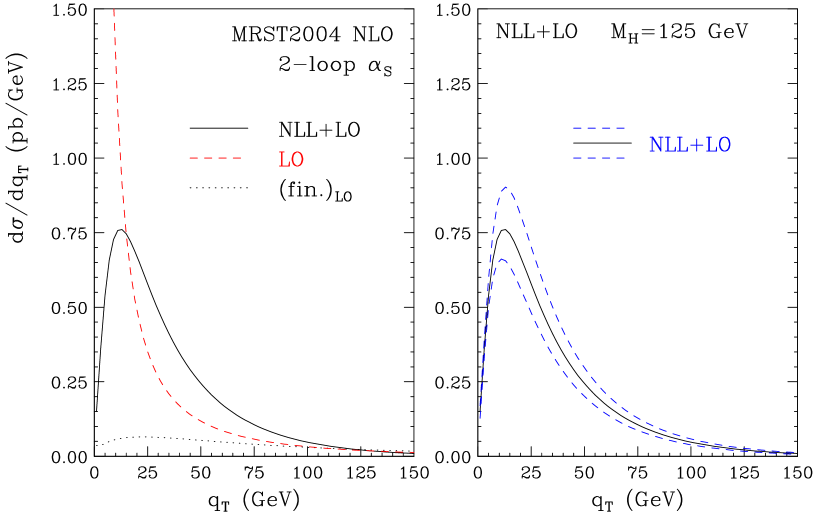
Figure 1: The $q_{T}$ spectrum at the LHC with $M_{H}=125$ GeV: (left) setting $\mu_{R}=\mu_{F}=Q=M_{H}$, the results at NLL+LO accuracy are compared with the LO spectrum and the finite component of the LO spectrum; (right) the uncertainty band from variations of the scales $\mu_{R}$ and $\mu_{F}$ at NLL+LO accuracy.

The NLL+LO spectrum with $M_{H}=125$ GeV is shown in Fig. 1. In the left-hand side, the full NLL+LO result (solid line) is compared with the LO one (dashed line) at the default scales $\mu_{F}=\mu_{R}=Q=M_{H}$. We see that the LO calculation diverges to $+\infty$ as $q_{T}\rightarrow 0$. The effect of the resummation, which is relevant below $q_{T}\sim 100$ GeV, leads to a physically well-behaved distribution: it has a kinematical peak at $q_{T}\sim 12$ GeV and vanishes as $q_{T}\rightarrow 0$. The LO finite component of the spectrum (dotted line), which is defined in Eq. (58), is also shown: as expected it dominates when $q_{T}\sim M_{H}$ and vanishes as $q_{T}\rightarrow 0$. Note, however, that the contribution of the finite component is sizeable in the intermediate-$q_{T}$ region (about 20% at $q_{T}\sim 50$ GeV) and not yet negligible at small values of $q_{T}$ (about 8% around the peak region). This underlies the importance of a careful and consistent matching between the resummed and fixed-order calculations. In the right-hand side of Fig. 1 we show the NLL+LO band as obtained by varying $\mu_{F}$ and $\mu_{R}$ simultaneously and independently in the range $0.5M_{H}\leq\mu_{F},\mu_{R}\leq 2M_{H}$ with the constraint $0.5\leq\mu_{F}/\mu_{R}\leq 2$ (the resummation scale is kept fixed at $Q=M_{H}$). The scale dependence increases from about $\pm 15\%$ at the peak to about $\pm 20\%$ at $q_{T}=100$ GeV. The integral over $q_{T}$ of the NLL+LO spectrum is in agreement with the value of the NLO total cross section to better than $1\%$, thus proving the numerical accuracy of the code.

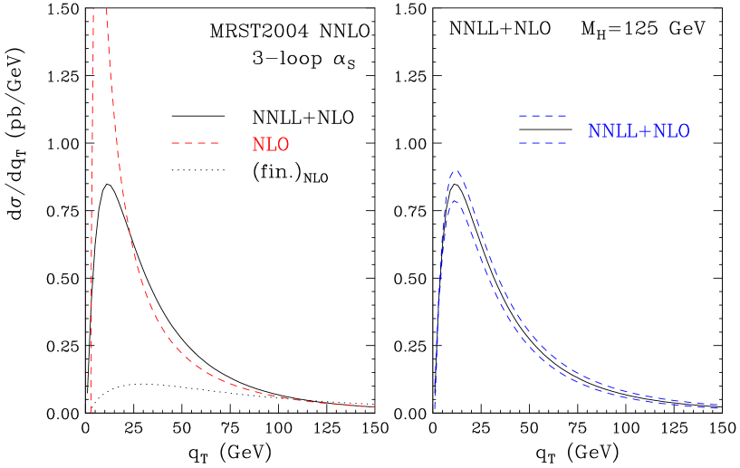
Figure 2: The $q_{T}$ spectrum at the LHC with $M_{H}=125$ GeV: (left) setting $\mu_{R}=\mu_{F}=Q=M_{H}$, the results at NNLL+NLO accuracy are compared with the NLO spectrum and the finite component of the NLO spectrum; (right) the uncertainty band from variations of the scales $\mu_{R}$ and $\mu_{F}$ at NNLL+NLO accuracy.

The NNLL+NLO results at the LHC are shown in Fig. 2. In the left-hand side, the full result (solid line) is compared with the NLO one (dashed line) at the default scales $\mu_{F}=\mu_{R}=Q=M_{H}$. The NLO result diverges to $-\infty$ as $q_{T}\rightarrow 0$ and, at small values of $q_{T}$, it has an unphysical peak (the top of the peak is above the vertical scale of the plot) that is produced by the numerical compensation of negative leading logarithmic and positive subleading logarithmic contributions. The resummed result is physically well-behaved at small $q_{T}$. The NLO finite component of the spectrum (dotted line), which is defined in Eq. (59), vanishes smoothly as $q_{T}\rightarrow 0$; its contribution amounts to about 10% in the peak region, about 17% at $q_{T}\sim 25$ GeV and about 35% at $q_{T}\sim 50$ GeV. This shows both the quality and the relevance of the matching procedure.

We find that the contribution of $A^{(3)}$ (recall from Sect. 2.3 that we are using an educated guess on the value of the coefficient $A^{(3)}$) to the resummed component can safely be neglected. The coefficient ${\cal H}_{N}^{H(2)}$ contributes significantly, and enhances the $q_{T}$ distribution by roughly $20\%$ in the region of intermediate and small values of $q_{T}$. The NNLL resummation effect starts to be visible below $q_{T}\sim 100$ GeV, and it increases the NLO result by about $25\%$ at $q_{T}=50$ GeV.

The right-hand side of Fig. 2 shows the scale dependence computed as in Fig. 1. The scale dependence is now about $8\%$ at the peak and increases to about $20\%$ at $q_{T}=100$ GeV.

To better illustrate the main features of the dependence on the scales $\mu_{R}$ and $\mu_{F}$, we present numerical results at two fixed values of $q_{T}$ in Figs. 3 and 4. In Fig. 3 we show our results at $q_{T}=50$ GeV and $M_{H}=125$ GeV. The scale dependence is analysed by varying the factorization and renormalization scales around the default value $M_{H}$. The plot on the left corresponds to the simultaneous variation of both scales, $\mu_{F}=\mu_{R}=\chi\,M_{H}$, whereas the plot in the centre (on the right) corresponds to the variation of the factorization (renormalization) scale $\mu_{F}=\chi_{F}\,M_{H}$ ($\mu_{R}=\chi_{R}\,M_{H}$) by fixing the other scale at the default value $M_{H}$.

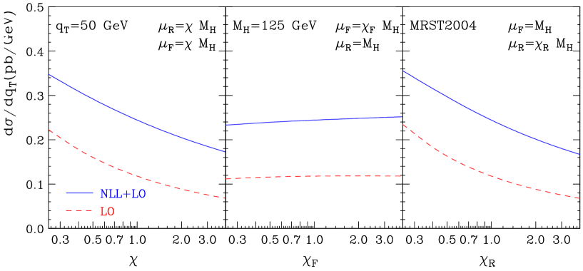
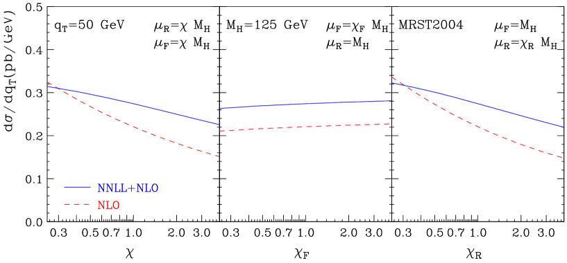
Figure 3: Scale dependence of the LHC cross section for Higgs boson production ($M_{H}=125$ GeV) at $q_{T}=50$ GeV. Results at a) (upper) LO, NLL+LO and b) (lower) NLO, NNLL+NLO accuracy.

As expected from the QCD running of $\alpha_{\mathrm{S}}$, the cross sections typically decrease when $\mu_{R}$ increases around the characteristic hard scale $M_{H}$, at fixed $\mu_{F}=M_{H}$. In the case of variations of $\mu_{F}$ at fixed $\mu_{R}=M_{H}$, we observe the opposite behaviour. This is not unexpected, since when $M_{H}=125$ GeV the cross section is mainly sensitive to partons with momentum fraction $x\sim 10^{-2}$, and in this $x$-range scaling violations of the parton densities are (moderately) positive. Varying the two scales simultaneously ($\mu_{F}=\mu_{R}$) leads to a partial compensation of the two different behaviours. As a result, the scale dependence is mostly driven by the renormalization scale, because the lowest-order contribution to the process is proportional to $\alpha_{\mathrm{S}}^{3}$, a (relatively) high power of $\alpha_{\mathrm{S}}$.

Comparing the LO with the NLL+LO results and the NLO with the NNLL+NLO results, we see that the scale dependence of the resummed results (solid lines) is smaller than that of the corresponding fixed-order results (dashed lines): the LO and NLL+LO curves have a comparable slope, but the NLL+LO results are higher; the NLO and NNLL+NLO results have smaller differences, but the slope of the NNLL+NLO curve is flatter. In summary, resummation reduces the scale dependence of the fixed-order calculations also in the region of intermediate values of $q_{T}$.

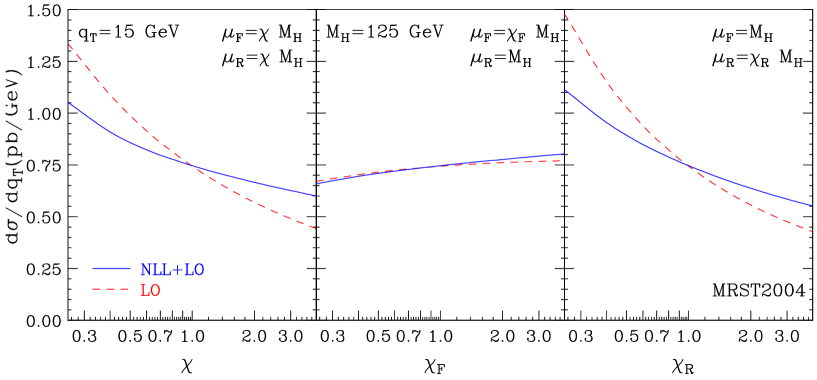
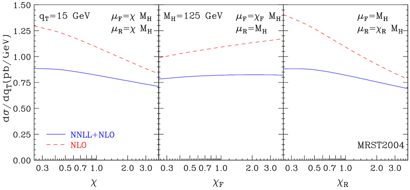
Figure 4: Scale dependence of the LHC cross section for Higgs boson production ($M_{H}=125$ GeV) at $q_{T}=15$ GeV. Results at a) (upper) LO, NLL+LO and b) (lower) NLO, NNLL+NLO accuracy.

In Fig. 4 we report analogous results at a smaller value of $q_{T}$, namely $q_{T}=15$ GeV. The qualitative behaviour is similar to the one in Fig. 3. In this region of small transverse momenta the fixed-order result is no longer reliable (see Figs. 1 and 2), but its relative scale dependence does not increase and is even smaller than at $q_{T}=50$ GeV. This is due to the fact that the fixed-order cross section is much larger than at higher values of $q_{T}$. The slope of the resummed results (solid lines) is sizeably flatter than that of the corresponding fixed-order results (dashed lines). We also notice a slight reduction in the scale dependence of the resummed results compared to Fig. 3, especially at NNLL+NLO accuracy.

In Fig. 5 the NLL+LO and NNLL+NLO bands shown in Figs. 1 and 2 are compared. We see that the NNLL+NLO band (solid lines) is smaller than the NLL+LO one (dashed lines) and overlaps with the latter at $q_{T}\raisebox{-2.58334pt}{\hbox to0.0pt{$\,\sim\,$\hss}}\raisebox{1.72218pt}{$\,<\,$}100$ GeV. This suggests a good convergence of the resummed perturbative expansion. This result is confirmed by the inset plot, that shows the NNLL+NLO band normalized to the NLL+LO result at central value of the scales. This $q_{T}$-dependent K factor,

$$K(q_{T})=\frac{d\sigma_{NNLL+NLO}(\mu_{F},\mu_{R})}{d\sigma_{NLL+LO}(\mu_{F}=\mu_{R}=M_{H})}\,,$$ (88)

is stable, around the values 1.1–1.2, in the central region of the inset plot, and it increases (decreases) drastically when $q_{T}\raisebox{-2.58334pt}{\hbox to0.0pt{$\,\sim\,$\hss}}\raisebox{1.72218pt}{$\,>\,$}50$ GeV ($q_{T}\raisebox{-2.58334pt}{\hbox to0.0pt{$\,\sim\,$\hss}}\raisebox{1.72218pt}{$\,<\,$}2$ GeV). In the large-$q_{T}$ region, the effect of perturbative higher-order corrections is known to be important [20–22]. At very small values of $q_{T}$, non-perturbative effects are definitely expected to be relevant. We observe that a naive rescaling of the NLL+LO result by a constant (i.e. independent of $q_{T}$) $K$ factor would not reproduce the NNLL+NLO result over the entire $q_{T}$-range.

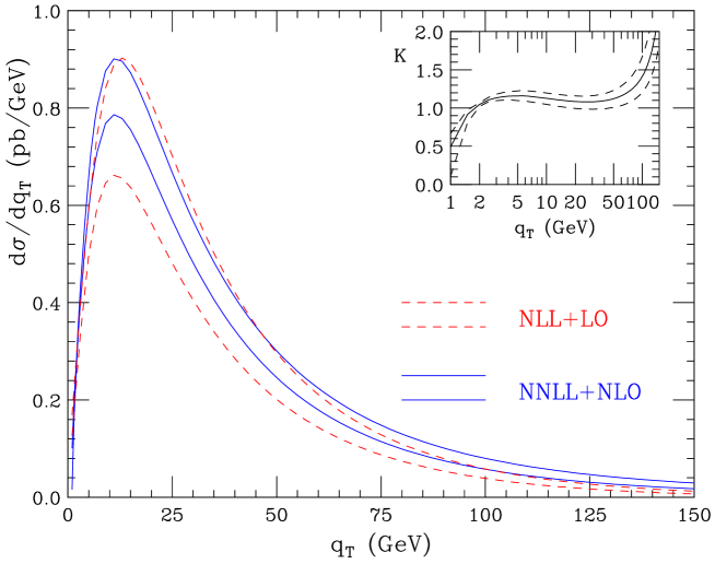
Figure 5: Comparison of the NLL+LO and NNLL+NLO bands ($M_{H}=125$ GeV). The inset plot shows the NNLL+NLO band normalized to the central value of the NLL+LO result.

The nice convergence of the resummed perturbative expansion suggested by Fig. 5 should be contrasted with the results in Fig. 6, where the corresponding fixed-order bands, computed as in Fig. 5, are shown. The results in Fig. 6 have no physical significance in the small-$q_{T}$ region, owing to the non-convergence of the fixed-order expansion herein. When $q_{T}\raisebox{-2.58334pt}{\hbox to0.0pt{$\,\sim\,$\hss}}\raisebox{1.72218pt}{$\,>\,$}25$ GeV, we see that the scale dependence of the NLO (LO) result is larger than the one of the corresponding NNLL+NLO (NLL+LO) result in Fig. 5. More importantly, we see that the LO and NLO bands do not overlap. This implies that the scale dependence enclosed by these bands certainly underestimates the true theoretical uncertainty from missing higher-order terms. Equivalently, we can say that the uncertainty of these fixed-order calculations is more reliably estimated by performing scale variations over a range of scales that is wider than that used in Fig. 6. All this indicates a poor convergence of the fixed-order perturbative expansion at intermediate values of $q_{T}$

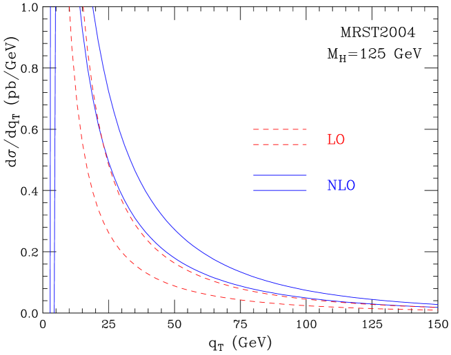
Figure 6: Comparison of the LO and NLO bands ($M_{H}=125$ GeV).

As mentioned at the beginning of this subsection, in our resummed calculations at NLL+LO and NNLL+NLO accuracy we use parton densities and $\alpha_{\mathrm{S}}$ at perturbative orders that are different from those customarily used in fixed-order calculations at LO and NLO, respectively. Indeed, the consistent procedure at large values of $q_{T}$ would be to use LO densities with 1-loop $\alpha_{\mathrm{S}}$ at the LO, and NLO densities with 2-loop $\alpha_{\mathrm{S}}$ at the NLO. We have also explained why our procedure is justified in the intermediate-$q_{T}$ region, and we have postponed the discussion on the large-$q_{T}$ region. To come back to this point, in Fig. 7 we compare our NLL+LO and NNLL+NLO results with the customary NLO results, which are obtained by using NLO parton densities and 2-loop $\alpha_{\mathrm{S}}$. We also include the corresponding bands, computed from scale variations. In the left-hand side we see that in the intermediate-$q_{T}$ region our NLL+LO result catches the bulk of the NLO effect. Obviously, at large $q_{T}$, the inclusion of NLO corrections is necessary. In the right-hand side, the calculations at NNLL+NLO accuracy and at the NLO are compared. In spite of the fact that the two calculations use different parton densities and $\alpha_{\mathrm{S}}$, the corresponding bands show a very good overlap when $q_{T}\sim M_{H}$. We thus conclude that, within the NLO theoretical uncertainty, the two calculations are perfectly compatible at the quantitative level in the large-$q_{T}$ region, $q_{T}\sim M_{H}$.

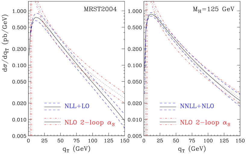
Figure 7: Comparison of the NLL+LO (left) and NNLL+NLO (right) bands with the NLO band computed by using NLO parton densities and 2-loop $\alpha_{\mathrm{S}}$.

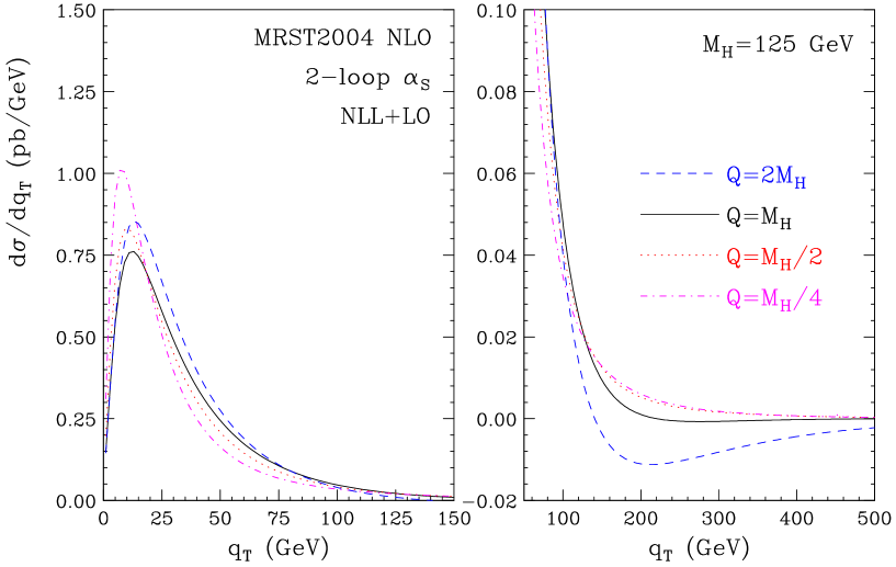
Figure 8: NLL+LO spectra for different choices of the resummation scale $Q$ at fixed $\mu_{R}=\mu_{F}=~{}M_{H}$.

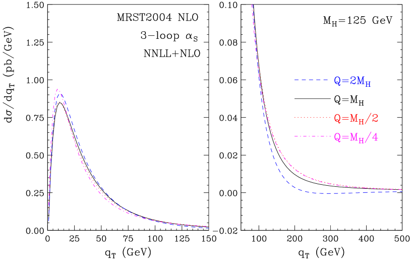
Figure 9: NNLL+NLO spectra for different choices of the resummation scale $Q$ at fixed $\mu_{R}=\mu_{F}=M_{H}$.

In Fig. 8 (Fig. 9) we plot the NLL+LO (NNLL+NLO) spectra for different choices of the resummation scale $Q$. We remind the reader that the resummation scale $Q$ has to be chosen of the order of $M_{H}$. Variations of the resummation scale around $M_{H}$ can be studied to estimate the uncertainty of the resummed calculation arising from not yet computed terms at higher logarithmic accuracy. In our quantitative study we consider four different values of $Q$, $Q=2M_{H},M_{H},M_{H}/2,M_{H}/4$.

We first comment on the behaviour at large transverse momenta, which is best visible looking at the plots on the right of Figs. 8 and 9. We see that the NLL+LO cross section can become negative if $Q=2M_{H}$. This behaviour should not be regarded as particularly worrisome: it takes place when $q_{T}>M_{H}$, where the use of the resummation formalism is not anymore justified. In general, the cross section has a better behaviour at large $q_{T}$ when the resummation scale has the values $Q=M_{H},M_{H}/2,M_{H}/4$. In particular, at large-$q_{T}$ the results of the fixed-order calculation at LO (NLO) accuracy are very well approximated by the NLL+LO (NNLL+NLO) calculation with $Q=M_{H}/2$; the line corresponding to the LO (NLO) results is not shown in the plot on the right of Fig. 8 (Fig. 9), since it is hardly distinguishable from the dotted and dot-dashed lines. The fact that the fixed-order behaviour at large $q_{T}$ is approximated better when $Q$ is smaller is not unexpected. By varying $Q$, we smoothly set the transverse-momentum scale below which the resummed logarithmic terms are mostly effective; when $Q$ is smaller, the resummation effects are confined to a range of smaller values of $q_{T}$.

To quantify the resummation-scale uncertainty on the cross section at small and intermediate values of $q_{T}$, we proceed as in the case of the renormalization and factorization scales, and we vary $Q$ by a factor of 2 up and down from a reference value. We choose the reference value $Q=M_{H}/2$, because of the better quality of the behaviour of the corresponding cross section at large $q_{T}$. From Fig. 8, we see that at NLL+LO accuracy a scale variation between $1/4M_{H}$ and $M_{H}$ produces a variation of the cross section of about $\pm 15\%$ in the region around the peak. At NNLL+NLO accuracy (Fig. 9) the resummation-scale dependence is much reduced: when $Q$ varies between $M_{H}/4$ and $M_{H}$ the change in the cross section at the peak is about $\pm 5\%$, i.e., smaller than the corresponding uncertainty from variations of the renormalization and factorization scales (see Fig. 2).

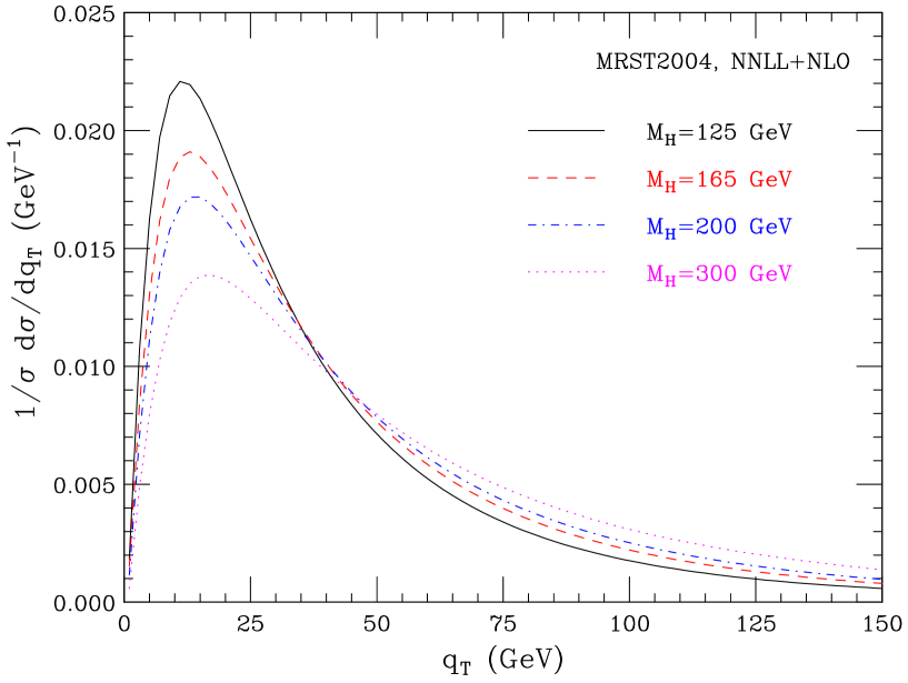
Figure 10: NNLL+NLO spectra for different values of the Higgs boson mass. The scales are set at the default value $\mu_{F}=\mu_{R}=Q=M_{H}$.

Throughout this section we used the MRST2004 set [70] of parton distribution functions at NLO and NNLO. The NLO and NNLO parton densities from Alekhin are currently being updated [71]. The CTEQ [72] and GRV [73] groups do not include sets of NNLO parton densities. The parton distribution sets of MRST, Alekhin and CTEQ include estimates of experimental uncertainties, which lead to effects below to about 5% on the total cross section for Higgs boson production at the LHC. We do not expect significantly different results in the case of the $q_{T}$ cross section at the LHC, and we refer to Ref. [17] for results and discussions about the effects of available parton densities on the total cross section.

The numerical results presented so far refer to the value $M_{H}=125$ GeV of the Higgs boson mass. By varying $M_{H}$, the typical features of the results are unchanged, the main difference being the decrease of the cross section as $M_{H}$ increases. In Fig. 10 we plot the NNLL+NLO spectra, normalized to the total cross section, for different values of the Higgs boson mass, $M_{H}=125,165,200$ and 300 GeV. For reference, the corresponding values of the NNLO total cross sections are $\sigma_{NNLO}=38.43,24.37,17.78$ and 10.03 pb. As expected, the $q_{T}$ distribution becomes harder as $M_{H}$ increases. The average value, $\langle q_{T}\rangle$, of the transverse momentum increases almost linearly with increasing $M_{H}$, and it is very roughly approximated by an effective lowest-order expression, $\langle q_{T}\rangle\sim C_{A}\alpha_{\mathrm{S}}(M_{H}^{2})\,M_{H}$.

The quantitative predictions presented up to now are obtained in a purely perturbative framework. It is known (see e.g. Ref. [29] and references therein) that the transverse-momentum distribution is affected by non-perturbative (NP) effects, which become important as $q_{T}$ becomes small. In impact parameter space, these effects are associated to the large-$b$ region. In our perturbative study the integral over the impact parameter turns out to be dominated by the region where $b\raisebox{-2.58334pt}{\hbox to0.0pt{$\,\sim\,$\hss}}\raisebox{1.72218pt}{$\,<\,$}0.1$–$0.2$ GeV^-1, larger values of $b$ being strongly suppressed by the resummation of the logarithmic terms in the gluon form factor. Thus we do not expect particularly-large NP effects in the case of Higgs boson production at the LHC. This expectation is in agreement with the findings in Refs. [40–44].

A customary way of modelling NP effects in the case of DY lepton-pair production is to introduce an NP transverse-momentum smearing of the distribution. This is implemented by multiplying the $b$-space perturbative form factor by an NP form factor. Several different parametrizations of the NP form factor are available in the literature [63, 74–77]; the corresponding NP parameters are obtained from global fits to DY data.

In the case of Higgs boson production, the estimate of NP effects is obviously more uncertain, since we cannot exploit available experimental data. In Ref. [78] we studied the impact of NP contributions on the $q_{T}$ spectrum of the Higgs boson, by applying the DY NP corrections of Refs. [74–76] to our resummed results at NLL accuracy. We also considered the effect of rescaling the DY NP coefficients by the factor $C_{A}/C_{F}$, to take into account the different colour charges of the initial-state partons ($q{\bar{q}}$ in the DY process, $gg$ in Higgs boson production) in the hard-scattering subprocess. Alternatively, we used the NP coefficients extracted in Ref. [43] from a fit of data on $\Upsilon$ production, a production process that is more sensitive to the gluon content of the colliding hadrons. All these different quantitative implementations of NP corrections, although certainly not fully justified, can give an idea of the size of the NP effects on the Higgs boson spectrum.

The results of Ref. [78] show that the impact of the NP effects on the NLL resummed distribution is definitely below $10\%$ for $q_{T}\raisebox{-2.58334pt}{\hbox to0.0pt{$\,\sim\,$\hss}}\raisebox{1.72218pt}{$\,>\,$}10$ GeV, and it decreases very rapidly as $q_{T}$ increases. Moreover, when $q_{T}\raisebox{-2.58334pt}{\hbox to0.0pt{$\,\sim\,$\hss}}\raisebox{1.72218pt}{$\,<\,$}10$ GeV, different parametrizations of the NP terms can lead to sizeably different relative effects, as a consequence of our present ignorance on the absolute value of the NP contributions.

In view of these results, in the present paper we limit ourselves to considering a simple parametrization of the NP contributions. We multiply the $b$-space resummed component ${\cal W}_{ab}^{H}(b,M,{\hat{s}})$ on the right-hand side of Eq. (10) by a NP factor, $S_{NP}$, which includes a gaussian smearing of the form

$$S_{NP}=\exp\{-g_{NP}\;b^{2}\}\,.$$ (89)

The NP coefficient $g_{NP}$ is varied in the range suggested by the study of Ref. [43]: $g_{NP}=1.67$–$5.64~{}{\rm GeV}^{2}$. Note that this procedure, with these values of $g_{NP}$, well approximates the quantitative spread of NP effects found in Ref. [78] at NLL accuracy. In Fig. 11 we plot the effect of the NP smearing on our best perturbative predictions, as given by the results at NNLL+NLO accuracy. The inner plot shows the relative deviation from the NNLL+NLO perturbative result, as defined by the ratio

$$\Delta=\frac{d\sigma_{NNLL+NLO}^{NP}-d\sigma_{NNLL+NLO}}{d\sigma_{NNLL+NLO}}\,,$$ (90)

where $d\sigma_{NNLL+NLO}^{NP}$ is the NNLL+NLO cross section, $d\sigma_{NNLL+NLO}$, supplemented with the NP form factor. We see that the NP effects give deviations from the purely perturbative result that are below $10\%$ for $q_{T}\raisebox{-2.58334pt}{\hbox to0.0pt{$\,\sim\,$\hss}}\raisebox{1.72218pt}{$\,>\,$}5$ GeV.

Figure 11: The NNLL+NLO perturbative results supplemented with the NP form factor in Eq. (89). The upper (lower) curve at small $q_{T}$ is obtained with $g_{NP}=1.67~{}{\rm GeV}^{2}\,(g_{NP}=5.64~{}{\rm GeV}^{2})$.

Comparing the inset plots in Figs. 5 and 11, we also notice that the inclusion of higher-order contributions (going from NLL+LO to NNLL+NLO) and of NP contributions have a qualitatively similar effect at intermediate and small values of transverse momenta: both contributions make the distribution harder. At the quantitative level, $\Delta$ is much smaller than $K-1$ when $q_{T}\raisebox{-2.58334pt}{\hbox to0.0pt{$\,\sim\,$\hss}}\raisebox{1.72218pt}{$\,>\,$}10$ GeV, while $\Delta$ and $K-1$ are comparable when $q_{T}\raisebox{-2.58334pt}{\hbox to0.0pt{$\,\sim\,$\hss}}\raisebox{1.72218pt}{$\,<\,$}10$ GeV. This points towards a non-trivial interplay between higher-order perturbative effects and NP effects at fixed value of the Higgs boson mass.

In summary, the comparison of the NLL+LO and NNLL+NLO results from small (around the peak region) to intermediate (say, roughly, $q_{T}\raisebox{-2.58334pt}{\hbox to0.0pt{$\,\sim\,$\hss}}\raisebox{1.72218pt}{$\,<\,$}M_{H}/3$) values of transverse momenta shows a nice convergence of the resummed QCD predictions for the $q_{T}$ spectrum of the Higgs boson at the LHC. From this comparison and from the effects of variations of the renormalization, factorization and resummation scales, we conclude that the perturbative QCD uncertainty of the NNLL+NLO results is uniformly of about $10\%$ over this range of transverse momenta. The perturbative and NP uncertainty increases at smaller values of $q_{T}$ (see Figs. 5 and 11); the perturbative uncertainty increases also at larger values of $q_{T}$ [20–22]. The perturbative uncertainty on the NNLO cross section [14], as estimated in the same manner (i.e. by comparing the NLO and NNLO results, and performing scale variations), is about 15% [17]. Our results on the $q_{T}$ spectrum are thus fully consistent with those on the total cross section, since the bulk of the events is concentrated at small and intermediate values of the Higgs boson $q_{T}$.

4 Conclusions

In this paper we have considered the transverse-momentum spectrum of generic systems of high-mass $M$ produced in hadron–hadron collisions. Following our previous work on the subject [33, 1], we have illustrated and discussed in detail a perturbative QCD formalism that allows us to resum the large logarithmic contributions in the small-$q_{T}$ region ($q_{T}\ll M$) and to consistently match the ensuing result to the fixed-order contributions in the large-$q_{T}$ region ($q_{T}\sim M$). The main features of our approach, that make it different from other implementations of $b$-space resummation presented in the literature, are summarized below.

• The resummation is performed at the level of the partonic cross section. The parton distributions are thus evaluated at the factorization scale $\mu_{F}$, which has to be chosen of the order of the hard scale $M$. The resummation formula is then organized in a form that is in close analogy with the case of event shapes variables in hard-scattering processes [54–57] and threshold resummation in hadronic collisions [58, 59]: the various classes of logarithmic contributions are controlled by the QCD coupling $\alpha_{\mathrm{S}}(\mu_{R}^{2})$ evaluated at the renormalization scale $\mu_{R}$. This procedure naturally allows us to perform a systematic study of renormalization- and factorization-scale dependence, as is customarily done in fixed-order calculations. This should be compared with the other implementations of $b$-space resummation, where the scale at which the parton distributions are evaluated is of the order of $1/b$, which also necessarily requires an extrapolation of the parton distributions in the NP region.

• The large logarithmic contributions are exponentiated in the form factor $\exp\{{\cal G}_{N}\}$, where the function ${\cal G}_{N}$ (see Eq. (2.2)) is universal: it does not depend on the produced high-mass system, and it only depends on the flavour of the partons involved in the hard-scattering subprocess. More precisely (see Appendix A), various process-independent form factors control the various partonic channels. The process dependence, as well as the factorization-scale and factorization-scheme dependence is fully included in the hard-scattering coefficient ${\cal H}_{N}$ (see Eq. (2.2)).

• We impose a constraint of perturbative unitarity through the replacement in Eq. (16): the $b$-space form factor $\exp\{{\cal G}_{N}({\widetilde{L}})\}$ is equal to unity at $b=0$. This constraint has a twofold purpose. On one hand, it avoids the introduction of unjustified higher-order contributions in the small-$b$ region, which are present [79] in standard implementations of $b$-space resummation. On the other hand, it allows us to recover the total cross section at the nominal fixed-order accuracy upon integration over $q_{T}$. Note that, as a consequence, perturbative uncertainties at intermediate values of $q_{T}$ are reduced.

The resummation formalism has been applied to the production of the SM Higgs boson in $pp$ collisions. We combined the most advanced perturbative information that is available at present for this process: NNLL resummation at small $q_{T}$ and fixed-order perturbation theory at NLO at large $q_{T}$. We developed a numerical code, named HqT [69], that performs the calculation at NLL+LO and NNLL+NLO accuracy. In Sect. 3.1 we have presented a selection of results that can be obtained by our program at LHC energies. Owing to the unitarity constraint, the integral of our spectra at NLL+LO (NNLL+NLO) correctly reproduces the total NLO (NNLO) cross sections. The results show a high stability with respect to scale variations and an increasing stability when going from NLL+LO to NNLL+NLO accuracy. As summarized at the end of Sect. 3.1, this suggests that the uncertainty from missing higher-order perturbative contributions is under good control.

Appendix A Appendix: Exponentiation in the multiflavour case

In Sects. 2.2 and 2.3, we have discussed the exponentiation structure of the resummed component of the $q_{T}$ distribution. To simplify the notation and the presentation, we have limited ourselves to illustrating the case in which the partonic scattering involves a single flavour of partons. This appendix is devoted to generalize the exponentiation to the case with partons of different flavours.

To obtain Eq. (2.3), the multiflavour analogue of Eq. (2.2), we start from the representation in Eq. (2.3) of the resummed partonic cross section ${\cal W}_{ab,\,N}^{F}$, and then we proceed as in Sect. 2.3. The main difference with respect to the steps in Eqs. (44)-(2.3) is that the solution of the QCD evolution equations (40) has the customary form

$${{\mbox{\boldmath$U$}}}_{N}(b_{0}^{2}/b^{2},Q^{2})=P\exp\left\{\int^{b_{0}^{2}/b^{2}}_{Q^{2}}\frac{dq^{2}}{q^{2}}\;{{\mbox{\boldmath$\gamma$}}}_{N}(\alpha_{\mathrm{S}}(q^{2}))\right\}\;\;,$$ (91)

where the symbol $P$ on the right-hand side denotes the path ordering expansion of the exponential matrix. Because of its matrix structure, the exponential in Eq. (91) has only a formal meaning. To recast Eq. (91) in a true exponential form, we can perform a systematic logarithmic expansion of the solution of the Altarelli–Parisi equations, by using a well-known method that dates back, at least, to Ref. [80].

The evolution operator in Eq. (91) can be written in the following form [80] (see also Ref. [81] for technical details):

$${{\mbox{\boldmath$U$}}}_{N}(b_{0}^{2}/b^{2},Q^{2})={{\mbox{\boldmath$V$}}}_{N}(\alpha_{\mathrm{S}}(b_{0}^{2}/b^{2}))\;{{\mbox{\boldmath$U$}}}_{N}^{(\rm LO)}(\alpha_{\mathrm{S}}(b_{0}^{2}/b^{2}),\alpha_{\mathrm{S}}(Q^{2}))\;{{\mbox{\boldmath$V$}}}_{N}^{-1}(\alpha_{\mathrm{S}}(Q^{2}))\;\;,$$ (92)

where ${{\mbox{\boldmath$U$}}}_{N}^{(\rm LO)}$ is determined by the lowest-order anomalous dimensions ${{\mbox{\boldmath$\gamma$}}}_{N}^{(1)}$,

$$\frac{d{{\mbox{\boldmath$U$}}}_{N}^{(\rm LO)}(\alpha_{\mathrm{S}},\alpha_{\mathrm{S}}^{\prime})}{d\ln\alpha_{\mathrm{S}}}=-\frac{1}{\beta_{0}}\;{{\mbox{\boldmath$\gamma$}}}_{N}^{(1)}\;{{\mbox{\boldmath$U$}}}_{N}^{(\rm LO)}(\alpha_{\mathrm{S}},\alpha_{\mathrm{S}}^{\prime})\;\;,$$ (93)

and the operator ${{\mbox{\boldmath$V$}}}_{N}$ fulfils the following differential equation:

$$\frac{d{{\mbox{\boldmath$V$}}}_{N}(\alpha_{\mathrm{S}})}{d\ln\alpha_{\mathrm{S}}}=\frac{1}{\beta(\alpha_{\mathrm{S}})}\;{{\mbox{\boldmath$\gamma$}}}_{N}(\alpha_{\mathrm{S}})\;{{\mbox{\boldmath$V$}}}_{N}(\alpha_{\mathrm{S}})+{{\mbox{\boldmath$V$}}}_{N}(\alpha_{\mathrm{S}})\;\frac{1}{\beta_{0}}\;{{\mbox{\boldmath$\gamma$}}}_{N}^{(1)}\;.$$ (94)

The evolution equation (93) can be solved by diagonalizing the anomalous dimensions matrix ${{\mbox{\boldmath$\gamma$}}}_{N}^{(1)}$, which has three different eigenvalues ${\gamma}_{i,\,N}^{(1)}$: one eigenvalue in the flavour non-singlet sector $(i={\rm NS})$, and two eigenvalues in the flavour singlet sector $(i=\pm)$. The solution of Eq. (93) is

$${{\mbox{\boldmath$U$}}}_{N}^{(\rm LO)}(\alpha_{\mathrm{S}}(b_{0}^{2}/b^{2}),\alpha_{\mathrm{S}}(Q^{2}))=\sum_{i={\rm NS},\pm}\left[\frac{\alpha_{\mathrm{S}}(Q^{2})}{\alpha_{\mathrm{S}}(b_{0}^{2}/b^{2})}\right]^{{\gamma}_{i,\,N}^{(1)}/\beta_{0}}\;{{\mbox{\boldmath$E$}}_{N}^{(i)}}\;\;,$$ (95)

where ${{\mbox{\boldmath$E$}}_{N}^{(i)}}$ denotes the projector onto the flavour eigenspace corresponding to the eigenvalue ${\gamma}_{i,\,N}^{(1)}$. By inspection of Eq. (94), we see that it can be solved by performing a perturbative expansion,

$${{\mbox{\boldmath$V$}}}_{N}(\alpha_{\mathrm{S}})={{\mbox{\boldmath$1$}}}+\sum_{n=1}^{\infty}\left(\frac{\alpha_{\mathrm{S}}}{\pi}\right)^{n}\;{{\mbox{\boldmath$V$}}}_{N}^{(n)}\;\;,$$ (96)

and the perturbative coefficients ${{\mbox{\boldmath$V$}}}_{N}^{(n)}$ are obtained in terms of the anomalous dimensions coefficients ${{\mbox{\boldmath$\gamma$}}}_{N}^{(k+1)}$ and the $\beta$ function coefficients $\beta_{k}$ with $k\leq n$. For example, the first-order coefficient ${{\mbox{\boldmath$V$}}}_{N}^{(1)}$ is given by

$${{\mbox{\boldmath$V$}}}_{N}^{(1)}=\sum_{i,j={\rm NS},\pm}\frac{1}{{\gamma}_{j,\,N}^{(1)}-{\gamma}_{i,\,N}^{(1)}-\beta_{0}}\;{{\mbox{\boldmath$E$}}_{N}^{(i)}}\;\left({{\mbox{\boldmath$\gamma$}}}_{N}^{(2)}-\frac{\beta_{1}}{\beta_{0}}\,{{\mbox{\boldmath$\gamma$}}}_{N}^{(1)}\right){{\mbox{\boldmath$E$}}_{N}^{(j)}}\;\;.$$ (97)

We now come back to the right-hand side of Eq. (2.3). The evolution operator ${{\mbox{\boldmath$U$}}}_{N}(b_{0}^{2}/b^{2},\mu_{F}^{2})$ is rewritten as ${{\mbox{\boldmath$U$}}}_{N}(b_{0}^{2}/b^{2},\mu_{F}^{2})={{\mbox{\boldmath$U$}}}_{N}(b_{0}^{2}/b^{2},Q^{2})\;{{\mbox{\boldmath$U$}}}_{N}(Q^{2},\mu_{F}^{2})$. Then ${{\mbox{\boldmath$U$}}}_{N}(b_{0}^{2}/b^{2},Q^{2})$ is replaced by the expression in Eq. (92). Equation (2.3) thus becomes

$${\cal W}_{ab,\,N}^{F}(b,M;\alpha_{\mathrm{S}}(\mu_{R}^{2}),\mu_{R}^{2},\mu_{F}^{2})=\sum_{c}\sigma_{c{\bar{c}},\,F}^{(0)}(\alpha_{\mathrm{S}}(M^{2}),M)\;H_{c}^{F}(\alpha_{\mathrm{S}}(M^{2}))$$

$$\quad\times\sum_{a_{2},\,b_{2}}\left[{{\mbox{\boldmath$V$}}}_{N}^{-1}(\alpha_{\mathrm{S}}(Q^{2}))\;{{\mbox{\boldmath$U$}}}_{N}(Q^{2},\mu_{F}^{2})\right]_{a_{2}a}\;\left[{{\mbox{\boldmath$V$}}}_{N}^{-1}(\alpha_{\mathrm{S}}(Q^{2}))\;{{\mbox{\boldmath$U$}}}_{N}(Q^{2},\mu_{F}^{2})\right]_{b_{2}b}$$

$$\quad\times\Bigl{\{}\;S_{c}(M,b)\;\sum_{a_{1},\,b_{1}}{\widetilde{C}}_{ca_{1},\,N}(\alpha_{\mathrm{S}}(b_{0}^{2}/b^{2}))\;{\widetilde{C}}_{{\bar{c}}b_{1},\,N}(\alpha_{\mathrm{S}}(b_{0}^{2}/b^{2}))\Bigr{.}$$ (98)

$$\quad\times\Bigl{.}\;U_{a_{1}a_{2},\,N}^{(\rm LO)}(\alpha_{\mathrm{S}}(b_{0}^{2}/b^{2}),\alpha_{\mathrm{S}}(Q^{2}))\;U_{b_{1}b_{2},\,N}^{(\rm LO)}(\alpha_{\mathrm{S}}(b_{0}^{2}/b^{2}),\alpha_{\mathrm{S}}(Q^{2}))\Bigr{\}}\;\;,$$

where we have defined the perturbative function

$${{\mbox{\boldmath$\widetilde{C}$}}}_{N}(\alpha_{\mathrm{S}})={{\mbox{\boldmath$C$}}}_{N}(\alpha_{\mathrm{S}})\;{{\mbox{\boldmath$V$}}}_{N}(\alpha_{\mathrm{S}})={{\mbox{\boldmath$1$}}}+\sum_{n=1}^{\infty}\left(\frac{\alpha_{\mathrm{S}}}{\pi}\right)^{n}\;{{\mbox{\boldmath$\widetilde{C}$}}}_{N}^{(n)}\;\;,$$ (99)

and inside the curly brackets we have collected all the factors, $S_{c},{{\mbox{\boldmath$\widetilde{C}$}}}_{N}$ and ${{\mbox{\boldmath$U$}}}_{N}^{(\rm LO)}$, that depend on the impact parameter $b$. These factors contain the logarithmically-enhanced contributions that have to be resummed and organized in exponential form. The factor $S_{c}$ can be rewritten as

$$S_{c}(M,b)=S_{c}(M,b_{0}/Q)\;\exp\left\{{\cal G}_{c}(\alpha_{\mathrm{S}}(\mu^{2}_{R}),L;M^{2}/\mu^{2}_{R},M^{2}/Q^{2})\right\}$$ (100)

where (see Eq. (31))

$${\cal G}_{c}(\alpha_{\mathrm{S}}(\mu^{2}_{R}),L;M^{2}/\mu^{2}_{R},M^{2}/Q^{2})=-\int_{b_{0}^{2}/b^{2}}^{Q^{2}}\frac{dq^{2}}{q^{2}}\left[A_{c}(\alpha_{\mathrm{S}}(q^{2}))\;\ln\frac{M^{2}}{q^{2}}+B_{c}(\alpha_{\mathrm{S}}(q^{2}))\right]\;\;.$$ (101)

The factor ${{\mbox{\boldmath$U$}}}_{N}^{(\rm LO)}$ is

$$U_{ab,\,N}^{(\rm LO)}(\alpha_{\mathrm{S}}(b_{0}^{2}/b^{2}),\alpha_{\mathrm{S}}(Q^{2}))=\sum_{i={\rm NS},\pm}E_{ab,\,N}^{(i)}\;\exp\left\{{\cal G}_{i,\,N}(\alpha_{\mathrm{S}}(\mu^{2}_{R}),L;M^{2}/\mu^{2}_{R},M^{2}/Q^{2})\right\}\;\;,$$ (102)

where (see Eq. (95))

$${\cal G}_{i,\,N}(\alpha_{\mathrm{S}}(\mu^{2}_{R}),L;M^{2}/\mu^{2}_{R},M^{2}/Q^{2})=\frac{{\gamma}_{i,\,N}^{(1)}}{\beta_{0}}\;\ln\frac{\alpha_{\mathrm{S}}(Q^{2})}{\alpha_{\mathrm{S}}(b_{0}^{2}/b^{2})}=\frac{{\gamma}_{i,\,N}^{(1)}}{\beta_{0}}\;\int_{b_{0}^{2}/b^{2}}^{Q^{2}}\frac{dq^{2}}{q^{2}}\;\beta(\alpha_{\mathrm{S}}(q^{2}))\;\;.$$ (103)

The factor ${\widetilde{C}}_{ca,\,N}$ can be written as

$${\widetilde{C}}_{ca,\,N}(\alpha_{\mathrm{S}}(b_{0}^{2}/b^{2}))={\widetilde{C}}_{ca,\,N}(\alpha_{\mathrm{S}}(Q^{2}))\;\exp\{{\cal G}_{ca,\,N}(\alpha_{\mathrm{S}}(\mu^{2}_{R}),L;M^{2}/\mu^{2}_{R},M^{2}/Q^{2})\}$$ (104)

where (see Eq. (37))

$${\cal G}_{ca,\,N}(\alpha_{\mathrm{S}}(\mu^{2}_{R}),L;M^{2}/\mu^{2}_{R},M^{2}/Q^{2})=-\int_{b_{0}^{2}/b^{2}}^{Q^{2}}\frac{dq^{2}}{q^{2}}\;\beta(\alpha_{\mathrm{S}}(q^{2}))\;\frac{d\ln{\widetilde{C}}_{ca,\,N}(\alpha_{\mathrm{S}}(q^{2}))}{d\ln\alpha_{\mathrm{S}}(q^{2})}\;\;.$$ (105)

Note a key point: Eq. (104) does not regard the flavour matrix ${{\mbox{\boldmath$\widetilde{C}$}}}_{N}$, but rather its matrix element ${\widetilde{C}}_{ca,\,N}$. Therefore, its right-hand side involves a true $c$-number exponential instead of a formal matrix exponential.

Inserting Eqs. (100), (102) and (104) in Eq. (A), we eventually obtain the final exponentiated result in Eq. (2.3), namely

$${\cal W}_{ab,\,N}^{F}(b,M;\alpha_{\mathrm{S}}(\mu_{R}^{2}),\mu_{R}^{2},\mu_{F}^{2}) =\sum_{\{I\}}{\cal H}_{ab,\,N}^{\{I\},\,F}\left(M,\alpha_{\mathrm{S}}(\mu_{R}^{2});M^{2}/\mu^{2}_{R},M^{2}/\mu^{2}_{F},M^{2}/Q^{2}\right)$$

$$\times\exp\{{\cal G}_{\{I\},\,N}(\alpha_{\mathrm{S}}(\mu^{2}_{R}),L;M^{2}/\mu^{2}_{R},M^{2}/Q^{2})\}\;\;,$$

where the sum extends over the following set of flavour indices:

$$\{I\}=c,{\bar{c}},i,j,a_{1},b_{1}\;.$$ (106)

The exponent ${\cal G}_{\{I\},\,N}$ of the universal form factor and the process-dependent hard factor ${\cal H}_{ab,\,N}^{\{I\},\,F}$ are

$${\cal G}_{\{I\},\,N}={\cal G}_{c}+{\cal G}_{i,\,N}+{\cal G}_{j,\,N}+{\cal G}_{ca_{1},\,N}+{\cal G}_{{\bar{c}}b_{1},\,N}\;\;,$$ (107)

$${\cal H}_{ab,\,N}^{\{I\},\,F} \left(M,\alpha_{\mathrm{S}}(\mu_{R}^{2});M^{2}/\mu^{2}_{R},M^{2}/\mu^{2}_{F},M^{2}/Q^{2}\right)=\sigma_{c{\bar{c}},\,F}^{(0)}(\alpha_{\mathrm{S}}(M^{2}),M)\;H_{c}^{F}(\alpha_{\mathrm{S}}(M^{2}))$$

$$\quad\times\;S_{c}(M,b_{0}/Q)\;\,{\widetilde{C}}_{ca_{1},\,N}(\alpha_{\mathrm{S}}(Q^{2}))\;\,{\widetilde{C}}_{{\bar{c}}b_{1},\,N}(\alpha_{\mathrm{S}}(Q^{2}))$$ (108)

$$\quad\times\;\left[{{\mbox{\boldmath$E$}}}_{N}^{(i)}\;{{\mbox{\boldmath$V$}}}_{N}^{-1}(\alpha_{\mathrm{S}}(Q^{2}))\;{{\mbox{\boldmath$U$}}}_{N}(Q^{2},\mu_{F}^{2})\right]_{a_{1}a}\;\left[{{\mbox{\boldmath$E$}}}_{N}^{(j)}\;{{\mbox{\boldmath$V$}}}_{N}^{-1}(\alpha_{\mathrm{S}}(Q^{2}))\;{{\mbox{\boldmath$U$}}}_{N}(Q^{2},\mu_{F}^{2})\right]_{b_{1}b}\;\;.$$

From Eqs. (101), (103) and (105) we see that ${\cal G}_{\{I\},\,N}$ in Eq. (107) has exactly the integral representation of Eq. (19). The logarithmic expansion (see Eq. (2.2)) of ${\cal G}_{c}$ and ${\cal G}_{i,\,N}$ starts at LL and NLL accuracy, respectively. The term ${\cal G}_{ca,\,N}$ starts at NLL accuracy in the flavour off-diagonal case $(c\neq a)$ and at NNLL accuracy in the flavour diagonal case $(c=a)$. The hard function ${\cal H}_{ab,\,N}^{\{I\},\,F}$ does not depend on the impact parameter $b$. It can be perturbatively expanded in powers of $\alpha_{\mathrm{S}}(\mu_{R}^{2})$ (with $\mu_{R}\sim M$), since the various factors on the right-hand side of Eq. (A) involve only scales $(M,Q,\mu_{F})$ that are of the order of the hard-scattering scale $M$.

We conclude this appendix with a comment on the solution (92) of the Altarelli–Parisi evolution equations and its relation with the resummation in Eq. (2.2) of the logarithmic contributions to the impact-parameter form factor $\exp\{{\cal G}_{\{I\},\,N}(\alpha_{\mathrm{S}},L)\}$.

The evolution operator ${{\mbox{\boldmath$U$}}}_{N}(b_{0}^{2}/b^{2},Q^{2})$ does not contribute to the LL function $g^{(1)}(\alpha_{\mathrm{S}}L)$ in Eq. (2.2). It starts to contribute to the resummation at the level of the NLL function $g_{N}^{(2)}(\alpha_{\mathrm{S}}L)$. Indeed, from Eqs. (102) and (103) we see that ${{\mbox{\boldmath$U$}}}_{N}^{(\rm LO)}(\alpha_{\mathrm{S}}(b_{0}^{2}/b^{2}),\alpha_{\mathrm{S}}(Q^{2}))$, the solution of the evolution equations at the lowest-perturbative order, contributes to the NLL terms $\alpha_{\mathrm{S}}^{n}L^{n}$. The higher-order corrections to the evolution equations are taken into account by the operator ${{\mbox{\boldmath$V$}}}_{N}(\alpha_{\mathrm{S}})$ in Eq. (92). The role of these corrections can be examined by organizing them in classes of logarithmic contributions $\alpha_{\mathrm{S}}^{k}(\alpha_{\mathrm{S}}L)^{n}$. Using the expansion in Eq. (96), Eq. (92) gives

$${{\mbox{\boldmath$U$}}}_{N}(b_{0}^{2}/b^{2},Q^{2})={{\mbox{\boldmath$U$}}}_{N}^{(\rm LO)}(\alpha_{\mathrm{S}}(b_{0}^{2}/b^{2}),\alpha_{\mathrm{S}}(Q^{2}))+{\cal O}(\alpha_{\mathrm{S}}^{n+2}L^{n+1})\;\;,\quad(n\geq 0)\;,$$ (109)

$${{\mbox{\boldmath$U$}}}_{N}(b_{0}^{2}/b^{2},Q^{2})={{\mbox{\boldmath$U$}}}_{N}^{(\rm NLO)}(\alpha_{\mathrm{S}}(b_{0}^{2}/b^{2}),\alpha_{\mathrm{S}}(Q^{2}))+{\cal O}(\alpha_{\mathrm{S}}^{n+3}L^{n+1})\;\;,\quad(n\geq 0)\;,$$ (110)

where ${{\mbox{\boldmath$U$}}}_{N}^{(\rm NLO)}$ is the customary solution [80, 81] of the evolution equations at NLO:

$${{\mbox{\boldmath$U$}}}_{N}^{(\rm NLO)}(b_{0}^{2}/b^{2},Q^{2}) ={{\mbox{\boldmath$U$}}}_{N}^{(\rm LO)}(\alpha_{\mathrm{S}}(b_{0}^{2}/b^{2}),\alpha_{\mathrm{S}}(Q^{2}))+\frac{\alpha_{\mathrm{S}}(b_{0}^{2}/b^{2})}{\pi}\;{{\mbox{\boldmath$V$}}}_{N}^{(1)}\;{{\mbox{\boldmath$U$}}}_{N}^{(\rm LO)}(\alpha_{\mathrm{S}}(b_{0}^{2}/b^{2}),\alpha_{\mathrm{S}}(Q^{2}))$$

$$-\frac{\alpha_{\mathrm{S}}(Q^{2})}{\pi}\;{{\mbox{\boldmath$U$}}}_{N}^{(\rm LO)}(\alpha_{\mathrm{S}}(b_{0}^{2}/b^{2}),\alpha_{\mathrm{S}}(Q^{2}))\;{{\mbox{\boldmath$V$}}}_{N}^{(1)}\;\;.$$ (111)

The terms denoted by ${\cal O}(\alpha_{\mathrm{S}}^{n+2}L^{n+1})$ on the right-hand side of Eq. (109) contribute at NNLL accuracy (they are of the same logarithmic accuracy as those in the function $\alpha_{\mathrm{S}}g_{N}^{(3)}(\alpha_{\mathrm{S}}L)$ in Eq. (2.2)). Analogously, the terms denoted by ${\cal O}(\alpha_{\mathrm{S}}^{n+3}L^{n+1})$ on the right-hand side of Eq. (109) contribute at NNNLL accuracy (they are of the same logarithmic accuracy as those in the function $\alpha_{\mathrm{S}}^{2}g_{N}^{(4)}(\alpha_{\mathrm{S}}L)$ in Eq. (2.2)). Therefore, to resum the NLL (NNLL) contributions to the form factor is sufficient to implement the solution of the evolution equations at the LO (NLO). Note, however, that, to be consistent with the resummed logarithmic expansion, the scale dependence of the running couplings $\alpha_{\mathrm{S}}(b_{0}^{2}/b^{2})$ and $\alpha_{\mathrm{S}}(Q^{2})$ in Eq. (109) (Eq. (110)) has to be evaluated at the NLO (NNLO).

Appendix B Appendix: Bessel transformation of logarithmic contributions

This appendix is devoted to the computation of the Bessel transformation of logarithmic contributions.

We recall the definition of the the functions ${\widetilde{I}}_{n}(q_{T}/Q)$ introduced in Eq. (74):

$${\widetilde{I}}_{n}(q_{T}/Q)=Q^{2}\int_{0}^{\infty}db\;\frac{b}{2}\,J_{0}(bq_{T})\;\ln^{n}\left(\frac{Q^{2}b^{2}}{b_{0}^{2}}+1\right)\;.$$ (112)

These integrals are easily evaluated in terms of derivatives of the corresponding generating function ${\widetilde{I}}(x;\epsilon)$:

$${\widetilde{I}}_{n}(x)=\lim_{\epsilon\rightarrow 0}\left(\frac{\partial}{\partial\epsilon}\right)^{n}{\widetilde{I}}(x;\epsilon)\;,$$ (113)

where

$${\widetilde{I}}(x;\epsilon)\equiv\sum_{n=0}^{\infty}\frac{1}{n!}\;\epsilon^{n}\;{\widetilde{I}}_{n}(x)\;\;.$$ (114)

Inserting Eq. (112) in the right-hand side of Eq. (114), we have

$${\widetilde{I}}(x;\epsilon)=\int_{0}^{\infty}dt\;\frac{t}{2}\,J_{0}(tx)\;\left(\frac{t^{2}}{b_{0}^{2}}+1\right)^{\epsilon}\;\;,$$ (115)

and this integral can be expressed [82] as follows in terms of $K_{\nu}(x)$, the modified Bessel function of imaginary argument (see Eq. (75)):

$${\widetilde{I}}(x;\epsilon)=-\left(\frac{2}{b_{0}x}\right)^{1+\epsilon}\;\frac{\epsilon\,b_{0}^{2}}{2\,\Gamma(1-\epsilon)}\;K_{1+\epsilon}(b_{0}x)\;\;.$$ (116)

Inserting Eq. (116) in Eq. (113) and using the relation

$$\Gamma(1-\epsilon)=\exp\Big{\{}\gamma_{E}\,\epsilon+\sum_{k=2}^{\infty}\frac{1}{k}\;\zeta_{k}\,\epsilon^{k}\Big{\}}\;\;,$$ (117)

where $\zeta_{n}$ is the Riemann zeta-function $(\zeta_{2}=\pi^{2}/6=1.645\dots,\zeta_{3}=1.202\dots)$, the integrals ${\widetilde{I}}_{n}(x)$ can straightforwardly be expressed in terms of the derivatives, $K_{1}^{(n)}(z)$, of the Bessel function with respect to its index $\nu$:

$$K_{1}^{(n)}(z)\equiv\left[\frac{\partial^{n}K_{\nu}(z)}{\partial\nu^{n}}\right]_{\nu=1}\;\;.$$ (118)

These derivatives have the following integral representation:

$$K_{1}^{(2n)}(z) =\int_{0}^{\infty}dt\;t^{2n}\;e^{-z\cosh t}\;\cosh t\;\;,$$ (119)

$$K_{1}^{(2n+1)}(z) =\frac{2n+1}{z}\int_{0}^{\infty}dt\;t^{2n}\;e^{-z\cosh t}\;\;,$$ (120)

which can simply be obtained from Eq. (75).

As discussed in Sect. 2.4, the computation of the finite component of the $q_{T}$ distribution requires the evaluation of the functions ${\widetilde{I}}_{n}(x)$ when $x>0$. In particular, the computation up to NLO (see Eq. (2.4)) requires ${\widetilde{I}}_{n}(x)$ with $n=1,2,3,4$; these functions are

$${\widetilde{I}}_{1}(x)=-\frac{b_{0}}{x}K_{1}(b_{0}x)\;,$$ (121)

$${\widetilde{I}}_{2}(x)=\frac{2b_{0}}{x}\left[K_{1}(b_{0}x)\;\ln x-K_{1}^{(1)}(b_{0}x)\right]\;,$$ (122)

$${\widetilde{I}}_{3}(x)=-\frac{3b_{0}}{x}\left[K_{1}(b_{0}x)\left(\ln^{2}x-\zeta_{2}\right)-2K^{(1)}_{1}(b_{0}x)\ln x+K_{1}^{(2)}(b_{0}x)\right]\;,$$ (123)

$${\widetilde{I}}_{4}(x)= \,\frac{4b_{0}}{x}\Big{[}K_{1}(b_{0}x)\;(\ln^{3}x-3\zeta_{2}\ln x+2\zeta_{3})-3K^{(1)}_{1}(b_{0}x)\;(\ln^{2}x-\zeta_{2})$$

$$+3K_{1}^{(2)}(b_{0}x)\;\ln x-K_{1}^{(3)}(b_{0}x)\Big{]}\;.$$ (124)

The functions ${\widetilde{I}}_{n}(x)$ diverge when $x\rightarrow 0$. To examine the divergent behaviour at small values of $x$, we introduce the functions ${\overline{I}}_{n}(x)$ and the corresponding generating function ${\overline{I}}(x;\epsilon)$:

$${\widetilde{I}}_{n}(x)={\overline{I}}_{n}(x)\left[1+{\cal O}(x^{2})\right]\;,$$ (125)

$${\widetilde{I}}(x;\epsilon)={\overline{I}}(x;\epsilon)\left[1+{\cal O}(x^{2})\right]\;.$$ (126)

Using the small-$x$ behaviour of the Bessel function $K_{1+\epsilon}(x)$ [82] and performing the small-$x$ limit of Eq. (116), we get

$${\overline{I}}(x;\epsilon)=-\,\epsilon\;D(\epsilon)\;\left(x^{2}\right)^{-1-\epsilon}\;,$$ (127)

where

$$D(\epsilon)=\left(\frac{2}{b_{0}}\right)^{\!2\epsilon}\;\frac{\Gamma(1+\epsilon)}{\Gamma(1-\epsilon)}=\exp\Big{\{}-2\sum_{k=1}^{\infty}\frac{\zeta_{2k+1}}{2k+1}\;\epsilon^{2k+1}\Big{\}}\;\;.$$ (128)

Note that the functions ${\overline{I}}_{n}(x)$ exactly correspond to the following Bessel transformations:

$${\overline{I}}_{n}(q_{T}/Q)=Q^{2}\int_{0}^{\infty}db\;\frac{b}{2}\,J_{0}(bq_{T})\;\ln^{n}\left(\frac{Q^{2}b^{2}}{b_{0}^{2}}\right)\;\;,$$ (129)

as can be checked by performing the limit $q_{T}\rightarrow 0$ of Eq. (112) or by verifying that the generating function in Eq. (127) has the following integral representation:

$${\overline{I}}(x;\epsilon)=\frac{1}{2}\;b_{0}^{-2\epsilon}\;\int_{0}^{\infty}dt\;t^{1+2\epsilon}\,J_{0}(tx)\;\;.$$ (130)

The relation between ${\overline{I}}_{n}(q_{T}/Q)$ and the small-$q_{T}$ limit of ${\widetilde{I}}_{n}(q_{T}/Q)$ is not unexpected in view of the discussion in Sect. 2.2. The integral in Eq. (112) originates from Eq. (129) after the replacement $L=\ln(Q^{2}b^{2}/b_{0}^{2})\rightarrow{\widetilde{L}}=\ln(1+Q^{2}b^{2}/b_{0}^{2})$ at the integrand level: when $q_{T}\rightarrow 0$, such a replacement has no effects on the singular behaviour at any logarithmic accuracy.

Though ${\overline{I}}_{n}(q_{T}/Q)$ and ${\widetilde{I}}_{n}(q_{T}/Q)$ coincide when $q_{T}\rightarrow 0$, they behave quite differently at very large values of $q_{T}$. When $x\rightarrow\infty$, from Eqs. (116) and (127) we get

$${\widetilde{I}}_{n}(x) =\left(-1\right)^{n}\,\frac{n}{x}\,{\sqrt{\frac{\pi b_{0}}{2x}}}\,e^{-b_{0}x}\;\ln^{n-1}\frac{b_{0}x}{2}\;\left[1+{\cal O}\left(\frac{1}{\ln x}\right)\right]\;\;,$$ (131)

$${\overline{I}}_{n}(x) =\left(-1\right)^{n}\,\frac{2^{n-1}n}{x^{2}}\,\;\ln^{n-1}x\;\left[1+{\cal O}\left(\frac{1}{\ln x}\right)\right]\;\;.$$ (132)

Note, in particular, that ${\widetilde{I}}_{n}(x)$ is integrable over $x^{2}$ when $x\rightarrow\infty$, whereas ${\overline{I}}_{n}(x)$ it is not.

The function ${\overline{I}}_{n}(x)$ can easily be computed by performing the $n$-th derivative of the generating function (127) with respect to the parameter $\epsilon$. To present the result, we first exclude the singular point $x=0$ and consider only the region $x>0$. Since the generating function depends on $x$ only through the factor $(x^{2})^{-1-\epsilon}$, $x^{2}\;{\overline{I}}_{n}(x)$ is simply a polynomial of degree $n-1$ in the variable $\ln x^{2}$:

$${\overline{I}}_{n}(x)=-\frac{1}{x^{2}}\;\sum_{k=0}^{n-1}\frac{n!}{k!\,(n-k-1)!}\;d_{k}\;\ln^{n-k-1}\frac{1}{x^{2}}\;\;,\quad x>0\;\;,$$ (133)

where the coefficients $d_{n}$ are obtained from Eq. (128):

$$d_{n}=\left[\left(\frac{d}{d\epsilon}\right)^{n}D(\epsilon)\right]_{\epsilon=0}\;\;.$$ (134)

The value of the first few coefficients is

$$d_{0}=1,\quad d_{1}=d_{2}=0,\quad d_{3}=-4\zeta_{3},\quad d_{4}=0,\quad d_{5}=-48\zeta_{5},\quad d_{6}=160\zeta_{3}^{2}\;\;.$$ (135)

The result in Eq. (133) agrees with that in Ref. [83], where one can find the numerical values of $d_{n}$ with $n\leq 19$ ($d_{n}=2^{n}{\overline{b}}_{n}(\infty)$, where ${\overline{b}}_{n}(\infty)$ are given in Table 1 of Ref. [83]). The small-$x$ limit of Eqs. (121)–(B) thus gives

$${\overline{I}}_{1}(x)=-\frac{1}{x^{2}}\;,\quad{\overline{I}}_{2}(x)=-\frac{2}{x^{2}}\ln\frac{1}{x^{2}}\;,\quad{\overline{I}}_{3}(x)=-\frac{3}{x^{2}}\ln^{2}\frac{1}{x^{2}}\;,\quad{\overline{I}}_{4}(x)=-\frac{4}{x^{2}}\left(\ln^{3}\frac{1}{x^{2}}-4\zeta_{3}\right)\;.$$ (136)

Note that, since $d_{1}=d_{2}=d_{4}=0$, ${\overline{I}}_{n}(x)$ can be expressed in a simple form to very high logarithmic accuracy. For example, we have:

$${\overline{I}}_{n}(x) =-\frac{n}{x^{2}}\left\{\;\ln^{n-1}\frac{1}{x^{2}}-\frac{2}{3}\,\zeta_{3}\,\frac{(n-1)!}{(n-4)!}\;\ln^{n-4}\frac{1}{x^{2}}-\frac{2}{5}\,\zeta_{5}\,\frac{(n-1)!}{(n-6)!}\;\ln^{n-6}\frac{1}{x^{2}}\right.$$

$$+\left.\frac{2}{9}\,\zeta_{3}^{2}\,\frac{(n-1)!}{(n-7)!}\;\ln^{n-7}\frac{1}{x^{2}}+{\cal O}\left(\ln^{n-8}\frac{1}{x^{2}}\right)\right\}\;\;,\quad\quad x>0\;\;.$$ (137)

We now discuss how to deal with the region around the singular point $x=0$. We first split the $x$ range in a large-$x$ $(x>x_{0})$ and a small-$x$ $(x\leq x_{0})$ region, where the parameter $x_{0}$ can be chosen arbitrarily. Setting $x_{0}=1$, we have

$${\overline{I}}_{n}(x)={\overline{I}}_{n}(x)\;\Theta(x-1)+{\overline{I}}_{n}(x)\;\Theta(1-x)\;.$$ (138)

In the large-$x$ region, which excludes the point $x=0$, ${\overline{I}}_{n}(x)$ is given by Eq. (133). In the small-$x$ region, to properly treat the singularity at $x=0$, we have to consider the generating function in Eq. (127) and use the expansion

$$(x^{2})^{-1-\epsilon}\;\Theta(1-x)=-\frac{1}{\epsilon}\;\delta(x^{2})+\left[\frac{1}{x^{2}}\,(x^{2})^{-\epsilon}\right]_{+}=-\frac{1}{\epsilon}\;\delta(x^{2})+\sum_{n=0}^{\infty}\frac{\epsilon^{n}}{n!}\left[\frac{1}{x^{2}}\ln^{n}\frac{1}{x^{2}}\right]_{+}\;\;,$$ (139)

where the plus-distribution is customarily defined by its action onto any function $h(x^{2})$ that is finite at $x=0$:

$$\int_{0}^{1}dx^{2}\;h(x^{2})\left[\frac{1}{x^{2}}\ln^{n}\frac{1}{x^{2}}\right]_{+}\equiv\int_{0}^{1}dx^{2}\;\frac{h(x^{2})-h(0)}{x^{2}}\;\ln^{n}\frac{1}{x^{2}}\;\;.$$ (140)

Therefore the generalization of Eq. (133) to include the point $x=0$ is

$${\overline{I}}_{n}(x)=d_{n}\;\delta(x^{2})-\;\sum_{k=0}^{n-1}\frac{n!}{k!\,(n-k-1)!}\;d_{k}\;\left[\,\frac{1}{x^{2}}\ln^{n-k-1}\frac{1}{x^{2}}\right]_{+}\;\;,\quad 0\leq x\leq 1\;\;.$$ (141)

The procedure described in Eqs. (138) and (139) can also be applied to properly define the integrals ${\widetilde{I}}_{n}(x)$ around the point $x=0$ in the small-$x$ region. Choosing $x_{0}=\infty$, the final result is equivalent to start from ${\widetilde{I}}_{n}(x>0)$, the expression of ${\widetilde{I}}_{n}(x)$ when $x\neq 0$ (for example, Eqs. (121)–(B)), and then introduce a generalized plus-prescription that acts in the entire range $0\leq x<\infty$. Formally we can write

$${\widetilde{I}}_{n}(x)=\left[{\widetilde{I}}_{n}(x>0)\right]_{+\infty}\;\;,$$ (142)

where the generalized plus-distribution is defined as

$$\int_{0}^{\infty}dx^{2}\;h(x^{2})\left[{\widetilde{I}}_{n}(x>0)\right]_{+\infty}\equiv\int_{0}^{\infty}dx^{2}\;\left[h(x^{2})-h(0)\right]\;{\widetilde{I}}_{n}(x>0)\;\;.$$ (143)

The choice $x_{0}=\infty$ to define the plus-prescription in the case of ${\widetilde{I}}_{n}$ is feasible since ${\widetilde{I}}_{n}(x)$ (unlike ${\overline{I}}_{n}(x)$) is integrable over $x^{2}$ when $x\rightarrow\infty$. This choice simplifies the definition of ${\widetilde{I}}_{n}$ since the right-hand side of Eq. (142) (unlike Eq. (141)) does not contain any contact term proportional to $\delta(x^{2})$. The contact term vanishes since the integrand factor $\ln^{n}(1+Q^{2}b^{2}/b_{0}^{2})$ in Eq. (112) vanishes at $b=0$. The vanishing of the contact term is thus ultimately related to the unitarity constraint in Eqs. (8) and (18).

Acknowledgements. The work of G.B. was supported by a postdoctoral fellowship of the French ministry for education and research. The work of D.dF. was supported in part by Fundación Antorchas, CONICET and UBACyT. D.dF. wishes to thank the INFN for support and hospitality during his visit at the Sezione di Firenze.

References

1. G. Bozzi, S. Catani, D. de Florian and M. Grazzini, Phys. Lett. B 564 (2003) 65.

2. For a review on Higgs physics in and beyond the Standard Model, see J. F. Gunion, H. E. Haber, G. L. Kane and S. Dawson, The Higgs Hunter’s Guide (Addison-Wesley, Reading, Mass., 1990); M. Carena and H. E. Haber, Prog. Part. Nucl. Phys.  50 (2003) 63; A. Djouadi, report LPT-ORSAY-05-17 [hep-ph/0503172], report LPT-ORSAY-05-18 [hep-ph/0503173].

3. R. Barate et al. [The LEP Collaborations and the LEP Working Group for Higgs boson searches], Phys. Lett. B 565 (2003) 61.

4. The LEP Collaborations, the LEP Electroweak Working Group and the SLD Electroweak and Heavy Flavour Groups, report LEPEWWG/2004–01 [hep-ex/0412015].

5. M. Carena et al., Report of the Tevatron Higgs working group, hep-ph/0010338; CDF and D0 Collaborations, Results of the Tevatron Higgs Sensitivity Study, report FERMILAB–PUB–03/320-E.

6. W. M. Yao [CDF and D0 Collaborations], report FERMILAB–CONF–04/307-E [arXiv:hep-ex/0411053].

7. CMS Coll., Technical Proposal, report CERN/LHCC/94-38 (1994); ATLAS Coll., ATLAS Detector and Physics Performance: Technical Design Report, Vol. 2, report CERN/LHCC/99-15 (1999).

8. S. Abdullin et al., report CMS-NOTE-2003-033; S. Asai et al., Eur. Phys. J. C 32S2 (2004) 19.

9. S. Dawson, Nucl. Phys. B 359 (1991) 283; A. Djouadi, M. Spira and P. M. Zerwas, Phys. Lett. B 264 (1991) 440.

10. M. Spira, A. Djouadi, D. Graudenz and P. M. Zerwas, Nucl. Phys. B 453 (1995) 17.

11. R. V. Harlander, Phys. Lett. B 492 (2000) 74; V. Ravindran, J. Smith and W. L. van Neerven, Nucl. Phys. B 704 (2005) 332.

12. S. Catani, D. de Florian and M. Grazzini, JHEP 0105 (2001) 025, JHEP 0201 (2002) 015.

13. R. V. Harlander and W. B. Kilgore, Phys. Rev. D 64 (2001) 013015.

14. R. V. Harlander and W. B. Kilgore, Phys. Rev. Lett.  88 (2002) 201801; C. Anastasiou and K. Melnikov, Nucl. Phys. B 646 (2002) 220; V. Ravindran, J. Smith and W. L. van Neerven, Nucl. Phys. B 665 (2003) 325.

15. C. Anastasiou, L. J. Dixon and K. Melnikov, Nucl. Phys. Proc. Suppl.  116 (2003) 193; C. Anastasiou, K. Melnikov and F. Petriello, report SLAC-PUB-10673 [hep-ph/0409088].

16. M. Kramer, E. Laenen and M. Spira, Nucl. Phys. B 511 (1998) 523.

17. S. Catani, D. de Florian, M. Grazzini and P. Nason, JHEP 0307 (2003) 028.

18. R. K. Ellis, I. Hinchliffe, M. Soldate and J. J. van der Bij, Nucl. Phys. B 297 (1988) 221; U. Baur and E. W. Glover, Nucl. Phys. B 339 (1990) 38.

19. V. Del Duca, W. Kilgore, C. Oleari, C. Schmidt and D. Zeppenfeld, Nucl. Phys. B 616 (2001) 367, Phys. Rev. D 67 (2003) 073003.

20. D. de Florian, M. Grazzini and Z. Kunszt, Phys. Rev. Lett.  82 (1999) 5209.

21. V. Ravindran, J. Smith and W. L. Van Neerven, Nucl. Phys. B 634 (2002) 247.

22. C. J. Glosser and C. R. Schmidt, JHEP 0212 (2002) 016.

23. C. Anastasiou, K. Melnikov and F. Petriello, report UH-511-1066-05 [hep-ph/0501130].

24. J. Smith and W. L. van Neerven, report YITP-SB-04-65 [hep-ph/0501098].

25. Y. L. Dokshitzer, D. Diakonov and S. I. Troian, Phys. Rep.  58 (1980) 269.

26. G. Parisi and R. Petronzio, Nucl. Phys. B 154 (1979) 427.

27. G. Curci, M. Greco and Y. Srivastava, Nucl. Phys. B 159 (1979) 451.

28. J. C. Collins and D. E. Soper, Nucl. Phys. B 193 (1981) 381 [Erratum-ibid. B 213 (1983) 545].

29. J. C. Collins and D. E. Soper, Nucl. Phys. B 197 (1982) 446.

30. J. Kodaira and L. Trentadue, Phys. Lett. B 112 (1982) 66, report SLAC-PUB-2934 (1982), Phys. Lett. B 123 (1983) 335.

31. G. Altarelli, R. K. Ellis, M. Greco and G. Martinelli, Nucl. Phys. B 246 (1984) 12.

32. J. C. Collins, D. E. Soper and G. Sterman, Nucl. Phys. B 250 (1985) 199.

33. S. Catani, D. de Florian and M. Grazzini, Nucl. Phys. B 596 (2001) 299.

34. S. Catani, E. D’Emilio and L. Trentadue, Phys. Lett. B 211 (1988) 335.

35. R. P. Kauffman, Phys. Rev. D 45 (1992) 1512.

36. D. de Florian and M. Grazzini, Phys. Rev. Lett. 85 (2000) 4678, Nucl. Phys. B 616 (2001) 247.

37. I. Hinchliffe and S. F. Novaes, Phys. Rev. D 38 (1988) 3475.

38. R. P. Kauffman, Phys. Rev. D 44 (1991) 1415.

39. C. P. Yuan, Phys. Lett. B 283 (1992) 395.

40. C. Balazs and C. P. Yuan, Phys. Lett. B 478 (2000) 192.

41. C. Balazs, J. Huston and I. Puljak, Phys. Rev. D 63 (2001) 014021.

42. E. L. Berger and J. w. Qiu, Phys. Rev. D 67 (2003) 034026, Phys. Rev. Lett.  91 (2003) 222003.

43. A. Kulesza and W. J. Stirling, JHEP 0312 (2003) 056.

44. A. Kulesza, G. Sterman and W. Vogelsang, Phys. Rev. D 69 (2004) 014012.

45. A. Gawron and J. Kwiecinski, Phys. Rev. D 70 (2004) 014003; G. Watt, A. D. Martin and M. G. Ryskin, Phys. Rev. D 70 (2004) 014012 [Erratum-ibid. D 70 (2004) 079902].

46. A. V. Lipatov and N. P. Zotov, hep-ph/0501172.

47. T. Sjostrand, P. Eden, C. Friberg, L. Lonnblad, G. Miu, S. Mrenna and E. Norrbin, Comput. Phys. Commun.  135 (2001) 238; T. Sjostrand, L. Lonnblad, S. Mrenna and P. Skands, report LU-TP-03-38 [hep-ph/0308153].

48. G. Marchesini, B. R. Webber, G. Abbiendi, I. G. Knowles, M. H. Seymour and L. Stanco, Comput. Phys. Commun.  67 (1992) 465; G. Corcella et al., JHEP 0101 (2001) 010, report CERN-TH-2001-173 [hep-ph/0107071].

49. S. Frixione and B. R. Webber, JHEP 0206 (2002) 029; S. Frixione, P. Nason and B. R. Webber, JHEP 0308 (2003) 007; S. Frixione and B. R. Webber, report CERN-TH-2003-207 [hep-ph/0309186].

50. G. Corcella and S. Moretti, Phys. Lett. B 590 (2004) 249.

51. C. Balazs, M. Grazzini, J. Huston, A. Kulesza and I. Puljak, hep-ph/0403052, published in M. Dobbs et al., hep-ph/0403100, p. 51, Proceedings of the Les Houches 2003 Workshop on Physics at TeV Colliders.

52. G.Bozzi, PhD Thesis, University of Florence, April 2004.

53. J. C. Collins, D. E. Soper and G. Sterman, in Perturbative Quantum Chromodynamics, ed. A.H. Mueller (World Scientific, Singapore, 1989), p. 1.

54. S. Catani, G. Turnock, B. R. Webber and L. Trentadue, Phys. Lett. B 263 (1991) 491.

55. S. Catani, L. Trentadue, G. Turnock and B. R. Webber, Nucl. Phys. B 407 (1993) 3.

56. M. Dasgupta and G. P. Salam, Eur. Phys. J. C 24 (2002) 213, JHEP 0208 (2002) 032.

57. A. Banfi, G. P. Salam and G. Zanderighi, JHEP 0408 (2004) 062.

58. G. Sterman, Nucl. Phys. B 281 (1987) 310; S. Catani and L. Trentadue, Nucl. Phys. B 327 (1989) 323, Nucl. Phys. B 353 (1991) 183.

59. S. Catani, M. L. Mangano, P. Nason and L. Trentadue, Nucl. Phys. B 478 (1996) 273.

60. D. de Florian and M. Grazzini, Nucl. Phys. B 704 (2005) 387.

61. O. V. Tarasov, A. A. Vladimirov and A. Y. Zharkov, Phys. Lett. B 93 (1980) 429; S. A. Larin and J. A. Vermaseren, Phys. Lett. B 303 (1993) 334.

62. E. Laenen, G. Sterman and W. Vogelsang, Phys. Rev. Lett.  84 (2000) 4296; A. Kulesza, G. Sterman and W. Vogelsang, Phys. Rev. D 66 (2002) 014011.

63. J. w. Qiu and X. f. Zhang, Phys. Rev. Lett.  86 (2001) 2724, Phys. Rev. D 63 (2001) 114011.

64. R. K. Ellis, W. J. Stirling and B. R. Webber, QCD and collider physics, (Cambridge University Press, Cambridge, 1996) and references therein.

65. A. Vogt, Phys. Lett. B 497 (2001) 228; C. F. Berger, Phys. Rev. D 66 (2002) 116002.

66. S. Moch, J. A. M. Vermaseren and A. Vogt, Nucl. Phys. B 688 (2004) 101, Nucl. Phys. B 691 (2004) 129.

67. C. T. H. Davies and W. J. Stirling, Nucl. Phys. B 244 (1984) 337.

68. K. G. Chetyrkin, B. A. Kniehl and M. Steinhauser, Phys. Rev. Lett.  79 (1997) 353.

69. http://arturo.fi.infn.it/grazzini/codes.html

70. A. D. Martin, R. G. Roberts, W. J. Stirling and R. S. Thorne, Phys. Lett. B 604 (2004) 61.

71. S. Alekhin, Phys. Rev. D 68 (2003) 014002, talk presented at EPS05, HEP2005 Europhysics Conference, Lisboa, July 2005.

72. J. Pumplin, D. R. Stump, J. Huston, H. L. Lai, P. Nadolsky and W. K. Tung, JHEP 0207 (2002) 012.

73. M. Gluck, E. Reya and A. Vogt, Eur. Phys. J. C 5 (1998) 461

74. C. T. H. Davies, B. R. Webber and W. J. Stirling, Nucl. Phys. B 256 (1985) 413.

75. G. A. Ladinsky and C. P. Yuan, Phys. Rev. D 50 (1994) 4239.

76. F. Landry, R. Brock, P. M. Nadolsky and C. P. Yuan, Phys. Rev. D 67 (2003) 073016.

77. A. V. Konychev and P. M. Nadolsky, report ANL-HEP-PR-05-52 [hep-ph/0506225].

78. G. Bozzi, S. Catani, D. de Florian and M. Grazzini, in K. A. Assamagan et al. [Higgs Working Group Collaboration], hep-ph/0406152, p. 14, proceedings of the Les Houches 2003 Workshop on Physics at TeV Colliders.

79. S. Frixione, P. Nason and G. Ridolfi, Nucl. Phys. B 542 (1999) 311.

80. W. Furmanski and R. Petronzio, Z. Phys. C 11 (1982) 293.

81. A. Vogt, report NIKHEF-04-011 [hep-ph/0408244].

82. I.S. Gradshteyn and I.M. Ryzhik, Tables of Integrals, Series and Products (Academic Press, San Diego, 2000).

83. A. Kulesza and W. J. Stirling, Nucl. Phys. B 555 (1999) 279.