Top Mode Standard Model in Six Dimensions

Abstract

We construct a top-mode standard model where the third generation fermions and the $SU(2)_{L}\times U(1)_{Y}$ gauge bosons are put on a 6-dimensional brane (5-brane) with the extra dimensions compactified on the TeV scale ($R_{5}^{-1}=R_{6}^{-1}\equiv R^{-1}=1-10\,{\rm TeV}$), while only the gluons live in a compactified 8-dimensional bulk ($R_{7}^{-1}=R_{8}^{-1}\equiv\Lambda\gg R^{-1}$). On the 5-brane, Kaluza-Klein (KK) modes of the bulk gluons give rise to induced four-fermion interactions which, combined with the gauge interactions, are shown to be strong enough to trigger the top quark condensate, based on the dynamics of 6-dimensional gauged Nambu-Jona-Lasinio (NJL) model. Moreover, we can use a freedom of the brane positions to tune the four-fermion coupling close to the critical line of 6-dimensional gauged NJL model, so that the gap equation can ensure the top condensate on the weak scale while keeping other fermions massless. There actually exists a scale (“tMAC scale”), $\Lambda_{\rm tM}=(7.8-11.0)R^{-1}$, where the running gauge couplings combined with the induced four-fermion interactions trigger only the top condensate while no bottom and tau condensates. Furthermore, presence of such explicit four-fermion interactions enables us to formulate straightforwardly the compositeness conditions at $\Lambda=\Lambda_{\rm tM}$, which, through the renormalization-group analysis, yields a prediction of masses of the top quark and the Higgs boson, $m_{t}=177-187\,\text{GeV}$ and $m_{H}=183-207\,\text{GeV}$.

I Introduction

The origin of mass is one of the most urgent problems in the modern particle physics. The Standard Model (SM) has a mysterious part, the electroweak symmetry breaking (EWSB), to give mass to the elementary particles. The EWSB via the elementary Higgs boson in the SM has many problems, fine-tuning problem, etc. Particularly, the SM does not tell us why only the top quark has a mass of order of the EWSB scale.

A simple solution was actually proposed much earlier than the discovery of the top quark with the mass being this large, namely the idea of top quark condensation which was proposed by Miransky, Tanabashi and Yamawaki (MTY) MTY89 , based on the phase structure of the gauged Nambu-Jona-Lasinio (NJL) model KMY89 ; ASTW , and independently by Nambu Nambu89 in a different context (see also Marciano89 ). In order to trigger the top quark condensate $\langle\bar{t}t\rangle$, MTY introduced explicit four-fermion interactions:

$${\cal L}_{4f}=G_{t}(\bar{\psi}_{L}^{i}t_{R})({\bar{t}}_{R}{\psi_{L}}_{i})+G_{b}(\bar{\psi}_{L}^{i}b_{R})({\bar{b}}_{R}{\psi_{L}}_{i})+G_{tb}\left(\epsilon^{ik}\epsilon_{jl}\bar{\psi}_{L}^{i}{\psi_{R}}_{j}\bar{\psi}_{L}^{k}{\psi_{R}}_{l}\right)+h.c.,$$ (1)

with $\psi_{L}=(t,b)_{L}$, and similarly for other generations. The dimensionless four-fermion couplings $g_{t}$ is defined as $G_{t}\equiv g_{t}(4\pi^{2})/[N_{c}\Lambda^{2}]$ and similarly for $g_{b}$ and $g_{tb}$.   The situation $m_{t}\gg m_{b},m_{c}$ is realized as the critical phenomenon, $m_{t}\neq 0$ while $m_{b}=m_{c}=\cdots=0$ as the first approximation. This takes place when

$$g_{t}>g^{\rm crit}>g_{b},\,g_{c},\cdots$$ (2)

where $g=g^{\rm crit}$ is the value on the critical line of second order phase transition of the gauged NJL model: KMY89 ; ASTW

$$g=g^{\rm crit}=\frac{1}{4}\left(1+\sqrt{1-\frac{\alpha}{\alpha^{\rm crit}}}\right)^{2}$$ (3)

with $\alpha=g^{2}/(4\pi)$ ($g$: gauge coupling const.) and $\alpha^{\rm crit}=\pi/3$. The gap equation (improved ladder Schwinger-Dyson (SD) equation) dictates that the top mass can be much smaller than the cutoff $m_{t}\ll\Lambda$ by tuning the four-fermion coupling arbitrarily close to the critical line $0<g_{t}-g^{\rm crit}\ll 1$. The model predicted a top mass of weak scale order by the Pagels-Stokar formula Pagels:hd evaluated through the solution of the gap equation and also predicted a scalar bound state $\bar{t}t$ which plays the role of the Higgs boson in the SM. Thus the model was called “top mode standard model”(TMSM). The TMSM was further formulated in an elegant fashion by Bardeen, Hill and Lindner (BHL) BHL:1989ds through the renormalization-group equations (RGE’s) of the SM combined with the compositeness condition. (For reviews of TMSM see Yamawaki96 ; Miransky:vk ; Hill:2002ap .)

However, the original TMSM has a few problems: The model needs ad hoc four-fermion interactions whose origin is not known. Furthermore, even if we assumed the cutoff, $\Lambda$, is the Planck scale, the predicted mass of the top quark is $m_{t}=220-250\,\text{GeV}$, somewhat larger than the experimental value MTY89 ; BHL:1989ds . If we avoided the fine-tuning by assuming $\Lambda$ is a few TeV, then we would get a disastrous prediction $m_{t}\sim 600\,\text{GeV}$.

As to the origin of the four-fermion interactions, an immediate possibility is the massive vector boson exchange Tanabashi:1989sz whose explicit model was given by the topcolor Hill:1991at where the massive vector bosons (colorons) are the gauge bosons of the spontaneously broken extra gauge symmetry (topcolor) $SU(3)_{1}\times SU(3)_{2}\to SU(3)_{c}$. Further on this line, a solution to the top mass problem was given by the top quark seesaw model (TSS) TSS:1997nm ; He:2001fz where a new vector-like massive $SU(2)_{L}$-singlet $\chi$-fermion (seesaw partner of the top quark) mixed with the $t_{R}$ pushes down the top mass. Note that the $S$ and $T$ parameter constraints from the precision electroweak experiments are quite insensitive to introduction of massive vector-like fermions which contribute to the electroweak symmetry breaking Maekawa:1994yd . Then there arise new questions: How does the topcolor symmetry breaking pattern occur? Where does the $\chi$-fermion come from?

As an attractive answer to the above questions, the SM (without Higgs fields) was embedded into higher dimensions with compactified extra dimensions Dobrescu:1998dg ; CDH:1999bg : The gluon Kaluza-Klein (KK) modes play the role of the topcolor yielding the top-mode four-fermion interactions, while the KK modes of the $t_{R}$ (vector-like massive fermions) playing the role of the $\chi$-fermion. Then the TMSM with compactified extra dimensions is essentially equivalent to TSS, although the diagonal mass $\bar{t}t$ does exist in contrast to the seesaw mechanism.

A more straightforward version of the TMSM with extra dimensions was proposed by Arkani-Hamed, Cheng, Dobrescu and Hall (ACDH) ACDH:2000hv : All the third generation fermions and the SM gauge bosons are put in the $D(=6,8,10,\cdots)$-dimensional bulk on the equal footing, while other fermions are fixed on the 3-brane. Note that the four-fermion couplings are totally replaced by the bulk SM gauge dynamics and hence are no longer freely adjusted. Although it was expected in Ref. ACDH:2000hv that the pure gauge dynamics of the bulk SM (without four-fermion interactions) may give rise to the top quark condensate, it was found HTY:2000uk ; Gusynin:2002cu , that the bulk QCD in six dimensions actually is not strong enough as to trigger the top quark condensate within the analysis based on the truncated KK effective theory DDG for the running of gauge couplings and the (improved) ladder Schwinger-Dyson (SD) equation. One might hope that including the bulk $U(1)_{Y}$ gauge interaction would enhance the attractive forces strong enough to trigger the top quark condensate. However, it was shown HTY2003 by the full analysis of the bulk SM including the bulk $SU(2)_{L}\times U(1)_{Y}$ gauge interactions that the $D=6$ version of the ACDH scenario does not realize the “topped MAC” (tMAC) where the top quark condensate is the most attractive channel (MAC), since then the strong $U(1)_{Y}$ interaction favors the tau condensate rather than the top quark condensate. Giving up the possibility of $D=6$ case, the tMAC analysis in Ref. HTY2003 showed that $D=8$ version yields a viable model, predicting the mass of the top quark and the Higgs boson, $m_{t}=172-175\,{\rm GeV},m_{H}=176-188\,{\rm GeV}$.

Is there no chance for the $D=6$ TMSM to survive, then? Quite recently, phase structure of the $D(=6,8,10,\cdots)$-dimensional gauged NJL model was revealed Gusynin:2004jp , which is similar to the four-dimensional one KMY89 , Eq.(3). The result suggests that the top quark condensates even for $D=6$ TMSM can be formed thanks to the additional four-fermion interactions as in the original TMSM in four dimensions. Although it might be a kind of drawback to introduce arbitrary ad hoc four-fermion interactions, here we instead follow the method of Ref. Dobrescu:1998dg ; CDH:1999bg to generate such four-fermion interactions on the 5-brane out of the gauge dynamics in higher dimensional bulk, namely the KK modes of the bulk gluons in 8 dimensions with compactified extra dimensions.

In this paper, based on the phase structure of the 6-dimensional gauged NJL model Gusynin:2004jp , we shall construct a TMSM on the 5-brane with the third generation fermions and the $SU(2)_{L}\times U(1)_{Y}$ gauge bosons living on the 5-brane with the extra dimensions compactified on $T^{2}/Z_{2}$ with TeV scale ($R_{5}^{-1}=R_{6}^{-1}\equiv R^{-1}=1-10\,{\rm TeV}$), while only the gluons live in the 8-dimensional bulk compactified on $T^{2}/Z_{2}$, ($R_{7}^{-1}=R_{8}^{-1}\equiv\Lambda\gg R^{-1}$), where $R_{D}$ are the radii of D-dimensional compactification. Fermions of the first and the second generations are fixed on the 3-brane. We shall show that the induced four-fermion coupling indeed exceeds the value on the critical line of the gauged NJL model for the top condensate to take place. Moreover, we have a freedom of choosing the brane position by exploiting the compactification based on $T^{2}/Z_{2}$ rather than $T^{2}$, which is crucial for two reasons: The top quark mass must be kept to be of weak scale via the SD gap equation by tuning the four-fermion coupling close to the critical line (given the values of the SM gauge couplings on the brane). In order to realize the top condensate but not the bottom condensate, we further need to tune the four-fermion coupling close to the critical line in such a way that the $U(1)_{Y}$ gauge interaction discriminates the top in the broken phase (above the critical line) and the bottom in the symmetric phase (below the critical line). Important point is that what is uniquely dictated by the bulk QCD coupling is the upper bound of the induced four-fermion coupling on the 5-brane, whereas the actual value of it can be tuned arbitrarily smaller than its upper bound thanks to a freedom of the brane positions of our compactification $T^{2}/Z_{2}$. Thus, as far as the upper bound exceeds the value on the critical line, we can tune the brane positions so that the SD gap equation can ensure the top mass on the weak scale much smaller than $\Lambda$, $m_{t}\ll\Lambda$,  while keeping other fermions massless (as a zeroth approximation). We actually find a tMAC scale $\Lambda_{\rm tM}$ where the running gauge couplings, combined with the induced four-fermion interactions, trigger only the top condensate while no bottom and tau condensates. The tMAC scale in this model reads $\Lambda_{\rm tM}=(7.8-11.0)R^{-1}$. Here we use the value of the critical binding strength in the nonlocal gauge in the SD equation Gusynin:2002cu ; Gusynin:2004jp , which is larger than the (“conservative”) one used in the previous analysis HTY2003 based on the the Landau gauge HTY:2000uk , and hence our conclusion on the existence of the tMAC scale is quite independent of the ambiguity in the SD equation analysis. (In Ref. HTY2003 there would have been no tMAC scale even for $D=8$, if the value of the nonlocal gauge were used.) Moreover, in contrast to the previous models ACDH:2000hv ; HTY2003 , presence of such explicit four-fermion interactions enables us to formulate straightforwardly the compositeness conditions at $\Lambda=\Lambda_{\rm tM}$ which, through the RGE analysis á la BHL BHL:1989ds , yields a prediction of masses of the top quark $m_{t}$ and the Higgs boson $m_{H}$, $m_{t}=177-187\,\text{GeV}$ and $m_{H}=183-207\,\text{GeV}$.

The paper is organized as follows. In Sec.II we recapitulate the binding strength of the SM gauge couplings on the 5-brane. In Sec.III, we derive four-fermion interactions on the 5-brane induced out of 8-dimensional bulk gluons and estimate the strength of them. In Sec.IV, we show that the induced four-fermion couplings and the SM gauge couplings for the top quark on the 5-brane are larger than the critical line value of the gauged NJL model in six dimensions in such a way that only the top condensate takes place, while other fermions do not condense. Moreover the freedom of the brane positions can be used to tune the four-fermion coupling arbitrary close to the critical line so that the gap equation keeps the top mass on the weak scale order. In Sec.V, based on the BHL procedure of the RGE’s and the compositeness condition, we predict the masses of top quark and Higgs boson for the 6-dimensional TMSM. Sec.VI is devoted to summary and discussions.

II Binding strength of the Standard Model gauge couplings on the 5-brane

Here we depict the result of the one-loop running of the bulk gauge couplings of the SM in the KK effective theory DDG used for the tMAC analysis in Ref. HTY2003 ($SU(2)_{L}$ gauge coupling is irrelevant to the binding strength for the condensate). First, one-loop RGEs of four-dimensional couplings QCD ($g_{3}$), $SU(2)_{L}$ ($g_{2}$) and $U(1)_{Y}$ ($g_{Y}$) below the compactification scale $R^{-1}_{D}$ are given by

$$(4\pi)^{2}\mu\frac{dg_{i}}{d\mu}=b_{i}\,g_{i}^{3},\quad(\mu<R^{-1}_{D}),$$ (4)

where $b_{3}=-7,b_{2}=-19/6,b_{Y}=41/6$. Above the compactification scale the RGEs of $D$-dimensional QCD, $SU(2)_{L}$ and $U(1)_{Y}$ couplings in the truncated KK effective theory DDG are given by

$$(4\pi)^{2}\mu\frac{dg_{i}}{d\mu}=b_{i}\,g_{i}^{3}+b_{i}^{\rm KK}(\mu)\,g_{i}^{3},\quad(\mu\geq R^{-1}_{D}),$$ (5)

where $b_{i}^{\rm KK}$ for one generation and one (composite) Higgs boson are

$$b_{3}^{\rm KK}(\mu) = -11\,N_{\rm KK}^{g}(\mu)+\frac{\delta}{2}\,N_{\rm KK}^{gs}(\mu)$$ (6)

$$+\frac{8}{3}\,N_{\rm KK}^{f}(\mu),$$

$$b_{2}^{\rm KK}(\mu) = -\frac{22}{3}\,N_{\rm KK}^{g}(\mu)+\frac{\delta}{3}\,N_{\rm KK}^{gs}(\mu)$$ (7)

$$+\frac{8}{3}\,N_{\rm KK}^{f}(\mu)$$

$$+\frac{1}{6}\,N_{\rm KK}^{h}(\mu),$$

$$b_{Y}^{\rm KK}(\mu)=\frac{40}{9}\,N_{\rm KK}^{f}(\mu)+\frac{1}{6}\,N_{\rm KK}^{h}(\mu),$$ (8)

with $\delta\equiv D-4$ and $N_{\rm KK}^{i}(\mu)(i=g,gs,f,h)$ being the total numbers of KK modes below $\mu$ for gauge bosons, gauge scalars, four-component fermions and composite Higgs bosons, respectively. We take the relation that $N_{\rm KK}^{i}(\mu)$ are

$$N_{\rm KK}^{i}(\mu)=\frac{1}{2^{\delta/2}}\frac{\pi^{\delta/2}}{\Gamma(1+\delta/2)}(\mu R_{D})^{\delta}.$$ (9)

The RGE’s can be solved with the inputs from Ref. PDG :

$$\alpha_{3}(M_{Z})=0.1172\,,$$ (10)

$$\alpha_{2}(M_{Z})=0.033822\,,$$ (11)

$$\alpha_{Y}(M_{Z})=0.010167,$$ (12)

where $\alpha_{i}(\equiv g_{i}^{2}/(4\pi))$ are the value at $\mu=M_{Z}(=91.1876\;{\text{GeV}})$.

We relate the four-dimensional gauge coupling, $g_{i}$, to the $D$-dimensional gauge coupling, $g_{D,i}$, at the compactification scale: $R_{D}^{-1}$ for $T^{\delta}/Z_{2}^{k}$ as

$$g_{D,i}^{2}=\frac{(2\pi R_{D})^{\delta}}{2^{k}}g_{i}^{2},$$ (13)

and define dimensionless $D$-dimensional coupling: $\hat{g}_{Di}(\mu)$ as

$$\hat{g}_{Di}^{2}(\mu)\equiv g_{Di}^{2}(\mu)\mu^{D-4}.$$ (14)

Hence we obtain

$$\hat{g}_{D,i}^{2}(\mu)=\frac{(2\pi R\mu)^{\delta}}{2^{k}}g_{i}^{2}.$$ (15)

By Eq.(5), Eq.(9) and Eq.(15), we find RGEs for the dimensionless $D$-dimensional couplings:

$$\mu\frac{d}{d\mu}\hat{g}_{D,i}=\frac{\delta}{2}\,\hat{g}_{D,i}+\left(1+\frac{\delta}{2}\right)\Omega_{\rm NDA}\,b^{\prime}_{i}\,\hat{g}_{D,i}^{3},\quad\mbox{for }\mu\gg R_{D}^{-1},$$ (16)

where

$$\Omega_{\rm NDA}\equiv\frac{1}{(4\pi)^{D/2}\Gamma(D/2)},$$ (17)

and

$$b^{\prime}_{3} = -11+\frac{\delta}{2}+\frac{4}{3}\cdot 2^{\delta/2},$$ (18)

$$b^{\prime}_{Y} = ~{}~{}\frac{20}{9}\cdot 2^{\delta/2}+\frac{1}{6}.$$ (19)

(As noted before, the $SU(2)_{L}$ coupling is irrelevant to the condensate.)

Eq.(16) implies that there exists a nontrivial ultraviolet fixed point (UVFP) for $\hat{g}_{D,i}$: $\hat{g}_{D*,i}$ HTY:2000uk (see also Agashe:2000nk ; Kazakov:2002jd ; Dienes:2002bg ):

$$\hat{g}_{D*,i}^{2}\Omega_{\rm NDA}=\frac{1}{-(1+2/\delta)\,b^{\prime}_{i}},$$ (20)

for $b^{\prime}_{i}<0$. For $D=6$ case with the compactification $D=6\rightarrow D=4$ as $T^{2}/Z_{2}(\delta=2,k=\delta/2=1)$, the UVFP of the six dimensional QCD coupling ($D=6,i=3$) is

$$\hat{g}_{6*,3}^{2}\Omega_{\rm NDA}=\frac{3}{44}.$$ (21)

Next, based on the one-gauge-boson-exchange approximation Raby:1979my , the binding strength of a scalar channel ($\bar{\psi}\chi$) is defined as

$$\kappa(\mu) \equiv -\hat{g}_{D,3}^{2}(\mu)\Omega_{\rm NDA}\mbox{\boldmath$T$}_{\bar{\psi}}\cdot\mbox{\boldmath$T$}_{\chi}$$ (22)

$$-\hat{g}_{D,2}^{2}(\mu)\Omega_{\rm NDA}\mbox{\boldmath$T^{\prime}$}_{\bar{\psi}}\cdot\mbox{\boldmath$T^{\prime}$}_{\chi}$$

$$-\hat{g}_{D,Y}^{2}(\mu)\Omega_{\rm NDA}Y_{\bar{\psi}}Y_{\chi},$$

where $T$, $T^{\prime}$ are the generators of $SU(3)_{c}$, $SU(2)_{L}$ respectively, and $Y$ is the hypercharge. $T$, $T^{\prime}$ fulfill

$$-\,\mbox{\boldmath$T$}_{\bar{\psi}}\cdot\mbox{\boldmath$T$}_{\chi}=\frac{1}{2}\left(C_{2}(\bar{\psi})+C_{2}(\chi)-C_{2}(\bar{\psi}\chi)\right),$$ (23)

with $C_{2}(r)$ being the quadratic Casimir for the representation $r$ of the SM gauge group on the 5-brane. Hence we calculate the binding strength $\kappa_{\alpha}(\mu)$ for each channel:

$$\kappa_{t}(\mu) = C_{F}\hat{g}_{D,3}^{2}(\mu)\Omega_{\rm NDA}+\frac{1}{9}\hat{g}_{D,Y}^{2}(\mu)\Omega_{\rm NDA},$$ (24)

$$\kappa_{b}(\mu) = C_{F}\hat{g}_{D,3}^{2}(\mu)\Omega_{\rm NDA}-\frac{1}{18}\hat{g}_{D,Y}^{2}(\mu)\Omega_{\rm NDA},$$ (25)

$$\kappa_{\tau}(\mu) = \phantom{C_{F}\hat{g}_{D,3}^{2}(\mu)\Omega_{\rm NDA}+\;\;\;}\frac{1}{2}\hat{g}_{D,Y}^{2}(\mu)\Omega_{\rm NDA},$$ (26)

for the $D-$dimensional top, bottom and tau condensate, respectively and $C_{F}=4/3$ is the quadratic Casimir of the fundamental representation of $SU(3)_{c}$. Note again that $SU(2)_{L}$ gauge interactions are opearative only on the left-handed fermions and hence do not contribute to the biding strength for the scalar channel. In Fig.1 the resultant running of the binding strengths in Ref.HTY2003 is depicted.

By using the improved ladder SD equation for the pure gauge dynamics on the 5-brane, Ref. HTY:2000uk ; Gusynin:2002cu estimated that the critical binding strength $\kappa_{D}^{\rm crit}(D=6)$ is

$$\kappa_{6}^{\rm crit}\left\{\begin{array}[]{ll}\simeq&0.122\hskip 5.69054pt(\text{the Landau gauge fixing}),\\ =&0.15\hskip 10.81204pt(\text{the nonlocal gauge fixing}).\\ \end{array}\right.$$ (29)

Condensation takes place in the channel where the $\kappa_{\alpha}(\mu)$ ($\alpha=t,b,\tau$) exceeds the critical value at certain $\mu$. When we increase the energy scale $\mu$, the dimensionless couplings and hence $\kappa_{\alpha}$ grow so that the $\kappa_{\alpha}$ in the MAC at certain point exceeds the $\kappa_{6}^{\rm crit}$. The Landau gauge estimate yields a value of $\kappa_{6}^{\rm crit}$ smaller than that of the nonlocal gauge and hence was used in Ref. HTY2003 as a conservative criterion for the top condensate. Shown by Fig. 1, $\kappa_{t}$ in the top channel does not exceed the critical binding strength before the tau channel $\kappa_{\tau}$ does, even if we exploited a conservative estimate of the Landau gauge fixing method. Hence, it was concluded HTY2003 for $D=6$ that within the pure gauge dynamics there is no energy scale region where the top quark condensate is the MAC (tMAC scale).

In what follows we shall consider a new situation where the induced four-fermion interactions arising from the bulk gluon interaction in addition to the gauge interactions on the 5-brane can give rise to existence of tMAC, even if we exploit the nonlocal gauge estimate of the $\kappa_{6}^{\rm crit}$. Actually, since the Landau gauge in the improved ladder SD equation has a problem with the chiral Ward-Takahashi identityKugo:1992pr , we here use the nonlocal gauge value. Thus our conclusion of the existence of the tMAC scale will be independent of the ambiguity of the SD equation analysis on the $\kappa_{6}^{\rm crit}$.

(a)       $R_{6}^{-1}=10\,\text{TeV}$ (b)       $R_{6}^{-1}=1\,\text{TeV}$

Figure 1: Binding strengths $\kappa_{\alpha}$ ($\alpha=t,b,\tau$) for the top, bottom and $\tau$ on the 5-brane: A compactification scale is (a) $R_{6}^{-1}=10\,\text{TeV}$ and (b) $R_{6}^{-1}=10\,\text{TeV}$. Note that the upper horizontal line is $\kappa_{6}^{\rm crit}$ by using the nonlocal gauge fixing method ($\kappa_{6}^{\rm crit}=0.15$) and the lower one is $\kappa_{6}^{\rm crit}$ by using the Landau gauge fixing method ($\kappa^{\rm crit}=0.122$)  HTY2003 ; Gusynin:2002cu .

III Induced four-fermion interactions on the 5-brane

Following Ref. CDH:1999bg , we first show that four-fermion interaction on the 5-brane are induced by gluonic KK-mode exchanges.

First let us consider a QCD Lagrangian on the 5-brane with the gluons in the seven-dimensional bulk for illustration:

$$\mathcal{L}_{7D}=\delta(x_{7}-x_{70})\bar{\psi}(X)i\Gamma^{M}D_{M}\psi(X).$$ (30)

where,

$$D_{M}=\partial_{M}-ig_{7,3}G^{a}_{M}(X,x_{7})T^{a},$$

with $M=(\mu,5,6),(\mu=0,1,2,3)$ and $X=(x,y),x=x_{\mu},y=x_{5,6}$ and $T^{a}\,(a=1,2,\cdots)$ are $SU(3)_{c}$ indexes. The above Lagrangian is gauge-invariant on the 5-brane $(M=\mu,5,6)$.

In order to compactify the seventh dimension, we impose boundary conditions ($S^{1}/Z_{2}$-compactification):

$$G_{M}(X,x_{7})=G_{M}(X,x_{7}+2\pi R_{7})$$ (31)

$$G_{M}(X,x_{7})=G_{M}(X,-x_{7})$$ (32)

Hence the gluons in the seven-dimensional bulk are decomposed as follows.

$$G_{M}(X,x_{7})=\frac{1}{\sqrt{2\pi R_{7}}}\Biggl{[}G_{M,0}(X)+\sqrt{2}\sum_{n=1}^{n_{\rm KK}}G^{[n]}_{M,c}(X)\cos\frac{nx_{7}}{R_{7}}\Biggr{]}.$$ (33)

Hereafter, we will call the gluons KK-modes “colorons”.

The induced four-fermion interactions on the 5-brane between the fermions on the 5-brane and colorons may be approximated by the one-coloron exchanges of the KK tower. By taking account of the brane position $x_{70}$, which represents where the 5-brane exists in the seven-dimensional bulk in the compactification of $S^{1}/Z_{2}$, we have an effective Lagrangian (gauged NJL model) in the 5-brane:

$$\mathcal{L}_{6D}=\bar{\psi}(X)i\Gamma^{M}D_{M,0}\psi(X)+\mathcal{L}_{\rm 4F},$$ (34)

where

$$D_{M,0} = \partial_{M}-ig_{6,3}G^{a}_{M,0}(X)T^{a},\quad g_{6,3}^{2}=2\frac{g^{2}_{7,3}}{2\pi R_{7}}\Bigg{|}_{\mu=\Lambda},$$ (35)

$$\mathcal{L}_{\rm 4F} = -\frac{2}{2\pi R_{7}}{\sum_{n=1}^{n_{\rm KK}}g^{2}_{7,3}(M_{n})\frac{\cos^{2}({nx_{70}}/R_{7})}{2M^{2}_{n}}}(\bar{\psi}\Gamma^{M}T^{a}\psi)(\bar{\psi}\Gamma_{M}T^{a}\psi),$$ (36)

where $M_{n}=n\Lambda$ ($\Lambda\equiv R_{7}^{-1}$) is the $n$-th KK mode mass and $n_{\rm KK}$ is the largest number of “colorons” we take into account (we implicitly assume that a bulk gauge theory is a cutoff theory, since it is unrenormalizable in the usual sense. Were it not for the ultraviolet cutoff of the bulk, $n_{\rm KK}$ would be infinite).

After Fierz transformations, scalar and pseudoscalar channels in (36) read

$$\begin{split}\mathcal{L}_{\rm 4F}^{\prime}&=\left[\frac{3}{4}\cdot\frac{1}{2}\cdot\frac{2}{2\pi R_{7}}{\sum_{n=1}^{n_{\rm KK}}g^{2}_{7,3}(M_{n})\frac{\cos^{2}({nx_{70}}/R_{7})}{2M^{2}_{n}}}\right]\cdot\Bigl{[}(\bar{\psi}\psi)^{2}+(\bar{\psi}i\Gamma_{A}\psi)^{2}\Bigr{]}\\ &=\frac{G_{6}^{(7)}}{2N_{c}}\cdot\Bigl{[}(\bar{\psi}\psi)^{2}+(\bar{\psi}i\Gamma_{A}\psi)^{2}\Bigr{]},\end{split}$$ (37)

where the factors 3/4 and 1/2 are from Fierz transformation for Lorentz indices and for the $SU(3)_{c}$ generator, respectively, $G_{6}^{(7)}$ is the six-dimensional induced four-fermion coupling from the seven-dimensional bulk gluons, and $\Gamma_{A}\equiv\Gamma^{0}\Gamma^{1}\Gamma^{2}\Gamma^{3}\Gamma^{4}\Gamma^{5}\Gamma^{6}$ is the 6-dimensional chirality matrix.

The summation in the coefficient of the four-fermion operator in (37) may be written as

$$\begin{split}\sum_{n=1}^{n_{\rm KK}}g^{2}_{7,3}(M_{n})\frac{\cos^{2}({nx_{70}}/R_{7})}{2M^{2}_{n}}&=\sum_{n=1}^{n_{\rm KK}}g^{2}_{7,3}(n\Lambda)\frac{\cos^{2}(nx_{70}/R_{7})}{2(n\Lambda)^{2}}\\ &=\frac{2\pi R_{7}}{2}\frac{g_{6,3}^{2}(\Lambda)}{2\Lambda^{2}}\sum_{n=1}^{n_{\rm KK}}\frac{\cos^{2}({nx_{70}}/R_{7})}{n^{5}},\end{split}$$ (38)

by considering the running effect of bulk gauge coupling:

$$g_{7,3}^{2}(n\Lambda)=\frac{g_{7,3}^{2}(\Lambda)}{n^{3}}=\frac{2\pi R_{7}}{2}\frac{g_{6,3}^{2}(\Lambda)}{n^{3}},$$ (39)

where we assumed dimensionless bulk gauge coupling $\hat{g}_{7,3}^{2}$ is on the UVFP: $g_{7,3}^{2}(\mu)=\hat{g}_{7,3}^{2}(\mu)/\mu^{3}=\hat{g}_{7*,3}^{2}/\mu^{3}$, since the dimensionless bulk QCD coupling approaches very quickly to the UVFP value HTY:2000uk (it is also true in the case without quark contributions). Then the induced four-fermion coupling is given by

$$\begin{split}\frac{G^{(7)}_{6}}{2N_{c}}&=\frac{g^{2}_{6,3}(\Lambda)}{2\Lambda^{2}}\cdot\frac{1}{2}\cdot\left[\frac{3}{4}\sum_{n=1}^{n_{\rm KK}}\frac{\cos^{2}({nx_{70}}/R_{7})}{n^{5}}\right]\\ &=\frac{g^{2}_{6,3}(\Lambda)}{2\Lambda^{2}}\cdot\frac{1}{2}\cdot c_{6}^{(7)}(x_{70}),\end{split}$$ (40)

where $c_{6}^{(7)}(x_{70})$ is the order $O(1)$ coefficient including factors from Fierz transformation, the running effects of gauge coupling and the number of KK-modes.

It is convenient to use the dimensionless four-fermion coupling

$$g_{D}\equiv 2^{D/2}G_{D}\Lambda^{D-2}\Omega_{\rm NDA}.$$ (41)

In our case $D=6$, the dimensionless induced four-fermion coupling from the 7-dimensional bulk gluons is

$$g_{6}^{(7)}=2^{3}G_{6}^{(7)}\Lambda^{4}\Omega_{\rm NDA}=c_{6}^{(7)}(x_{70})\cdot 2^{2}N_{c}\cdot\hat{g}^{2}_{6,3}(\Lambda)\Omega_{\rm NDA}=c_{6}^{(7)}(x_{70})\cdot\frac{3N_{c}}{11},$$ (42)

where we noted that the dimensionless gauge coupling $\hat{g}_{6,3}(\Lambda)^{2}$ defined by Eq.(14) may be evaluated by the value at the UVFP; $\hat{g}_{6,3}(\Lambda)^{2}\Omega_{\rm NDA}\simeq\hat{g}_{6*,3}\Omega_{\rm NDA}=3/44$ as given in Eq. (21). As to the evaluation of $c_{6}^{(7)}$, sum of an infinite tower of KK modes in this case happen to be given explicitly by a finite number, although we implicitly assume that a bulk gauge theory is a cutoff theory. Then we can estimate the upper bound of $c_{6}^{(7)}$ exactly,

$$\begin{split}c_{6}^{(7)}(x_{70})&=\frac{3}{4}\sum_{n=1}^{n_{\rm KK}}\frac{1}{n^{5}}\cos^{2}\frac{nx_{70}}{\Lambda^{-1}}\\ &<c_{6}^{(7)}(x_{70}=0)<\frac{3}{4}\sum_{n}^{\infty}\frac{1}{n^{5}}=\frac{3}{4}\zeta(5),\end{split}$$ (43)

hence the upper bound of $g_{6}^{(7)}$ ($N_{c}=3$) is given by

$$g_{6}^{(7)}=\frac{3N_{c}}{11}c_{6}^{(7)}(x_{70})<\frac{27}{44}\zeta(5)=0.636297,$$ (44)

which would have a chance to fulfill the condition of the condensation $g_{6}^{(7)}>g_{6}^{\rm crit}$, where $g_{6}^{\rm crit}$ ($1/2<g_{6}^{\rm crit}<2$) is the value (depending on the gauge binding strength $\kappa$) on the critical line of the 6-dimensional gauged NJL model Gusynin:2004jp (see later discussion in Sec. IV). However, we shall later show that actual possible $g_{6}^{\rm crit}$ required for the top condensate without tau condensate (tMAC scale condition) is $g_{6}^{\rm crit}>1.104$ (see Eq.(81)), which is not satisfied even by the upper limit in Eq.(44). Then the $D=7$ bulk gluons are not enough for producing the four-fermion interaction strong enough to trigger the top condensation while forbidding the tau condensate.

By this point we may remark that if we estimate the sum only by the lowest KK-mode or only up till the 4-th KK mode, $c_{6}^{(7)}(0)$ is given by

$$c_{6,\rm lowest}^{(7)}(0) = \frac{3}{4},$$ (45)

$$c_{6,\rm 4-th}^{(7)}(0) = 0.777256\sim\frac{3}{4}\zeta(5)=0.777696.$$ (46)

Hence, the summation of all the KK-mode effects is nearly equal to the summation only up till the 4-th effects.

Let us now consider the case of the gluons in the eight-dimensional bulk. As in the above derivation, after the seventh and eighth dimensions are compactified ($D=8\rightarrow D=6$) on $T^{2}/Z_{2}$, four-fermion interactions on the 5-brane are induced by the gluon Kaluza-Klein(KK) modes exchange.

The Lagrangian reads:

$$\mathcal{L}_{8D}=\delta(x_{7}-x_{70})\delta(x_{8}-x_{80})\bar{\psi}(X)i\Gamma^{M}D_{M}\psi(X),$$ (47)

where

$$D_{M}=\partial_{M}-ig_{8,3}G^{a}_{M}(x,y,z)T^{a},$$

with $x=x_{\mu},y=x_{5,6},z=x_{7,8},X=x,y$. This Lagrangian is gauge invariant on the 5-brane$(M=\mu,5,6)$. In order to compactify the seventh and eighth dimensions, we impose the boundary conditions ($T^{2}/Z_{2}$-compactification):

$$G_{M}(X,x_{7},x_{8}) = G_{M}(X,x_{7}+2\pi R_{7},x_{8})$$

$$= G_{M}(X,x_{7},x_{8}+2\pi R_{8}),$$

$$G_{M}(X,x_{7},x_{8}) = G_{M}(X,-x_{7},-x_{8}).$$ (49)

Hence the bulk gluons $G_{M}$ are decomposed as follows ($R_{7}=R_{8}=\Lambda^{-1}$).

$$\begin{split}G_{M}(X,x_{7},x_{8})=\frac{1}{2\pi\Lambda^{-1}}\Biggl{[}G_{M,00}(X)&+\sqrt{2}\sum_{n=1}^{n_{\rm KK}}G^{[n]}_{M,c0}(X)\cos\frac{nx_{7}}{\Lambda^{-1}}\\ &+\sqrt{2}\sum_{n=1}^{n_{\rm KK}}G^{[n]}_{M,0c}(X)\cos\frac{nx_{8}}{\Lambda^{-1}}\\ &+2\sum_{n_{1},n_{2}=1}^{n_{\rm KK}}G^{[n_{1},n_{2}]}_{M,cc}(X)\cos\frac{n_{1}x_{7}}{\Lambda^{-1}}\cos\frac{n_{2}x_{8}}{\Lambda^{-1}}\\ &+2\sum_{n_{1},n_{2}=1}^{n_{\rm KK}}G^{[n_{1},n_{2}]}_{M,ss}(X)\sin\frac{n_{1}x_{7}}{\Lambda^{-1}}\sin\frac{n_{2}x_{8}}{\Lambda^{-1}}\Biggr{]}.\end{split}$$ (50)

From the interaction between the fermions on the 5-brane and $G_{M}$, we derive four-fermion interactions on the 5-brane via one-coloron exchange. In consequence, we have

$$\mathcal{L}_{6D}=\bar{\psi}(X)i\Gamma^{M}D_{M,00}\psi(X)+\mathcal{L}_{\rm 4F},$$ (51)

with

$$D_{M,00}=\partial_{M}-ig_{6,3}G^{a}_{M,00}(X)T^{a},\quad g_{6,3}^{2}=2\frac{g^{2}_{8,3}}{(2\pi\Lambda^{-1})^{2}}\Bigg{|}_{\mu=\Lambda}$$ (52)

and

$$\begin{split}\mathcal{L}_{\rm 4F}=-\frac{2}{(2\pi\Lambda^{-1})^{2}}&\Bigl{[}\sum_{n=1}^{n_{\rm KK}}g^{2}_{8,3}\frac{\cos^{2}({nx_{70}}/\Lambda^{-1})}{2M^{2}_{n}}+\sum_{n=1}^{n_{\rm KK}}g^{2}_{8,3}\frac{\cos^{2}({nx_{80}}/\Lambda^{-1})}{2M^{2}_{n}}\\ &+2\sum_{n_{1},n_{2}=1}^{n_{\rm KK}}g^{2}_{8,3}\frac{\cos^{2}({n_{1}x_{70}}/\Lambda^{-1})\cos^{2}({n_{2}x_{80}}/\Lambda^{-1})}{2M^{2}_{\vec{n}}}\\ &+2\sum_{n_{1},n_{2}=1}^{n_{\rm KK}}g^{2}_{8,3}\frac{\sin^{2}({n_{1}x_{70}}/\Lambda^{-1})\sin^{2}({n_{2}x_{80}}/\Lambda^{-1})}{2M^{2}_{\vec{n}}}\Bigr{]}\times(\bar{\psi}\Gamma^{M}T^{a}\psi)(\bar{\psi}\Gamma_{M}T^{a}\psi).\end{split}$$ (53)

Furthermore, after the Fierz transformations, scalar and pseudoscalar channels in (53) are

$$\mathcal{L}_{\rm 4F}^{\prime} = \frac{3}{4}\cdot\frac{1}{2}\cdot\frac{2}{(2\pi\Lambda^{-1})^{2}}\Bigl{[}{\sum_{n=1}^{n_{\rm KK}}g^{2}_{8,3}\frac{\cos^{2}({nx_{70}}/\Lambda^{-1})}{2M^{2}_{n}}}+{\sum_{n=1}^{n_{\rm KK}}g^{2}_{8,3}\frac{\cos^{2}({nx_{80}}/\Lambda^{-1})}{2M^{2}_{n}}}$$ (54)

$$\hskip 56.9055pt+2{\sum_{n_{1},n_{2}=1}^{n_{\rm KK}}g^{2}_{8,3}\frac{\cos^{2}({n_{1}x_{70}}/\Lambda^{-1})\cos^{2}({n_{2}x_{80}}/\Lambda^{-1})}{2M^{2}_{\vec{n}}}}$$

$$\hskip 56.9055pt+2{\sum_{n_{1},n_{2}=1}^{n_{\rm KK}}g^{2}_{8,3}\frac{\sin^{2}({n_{1}x_{70}}/\Lambda^{-1})\sin^{2}({n_{2}x_{80}}/\Lambda^{-1})}{2M^{2}_{\vec{n}}}}\Bigr{]}\times\Bigl{[}(\bar{\psi}\psi)^{2}+(\bar{\psi}i\Gamma_{A}\psi)^{2}\Bigr{]},$$

$$= \frac{G_{6}^{(8)}}{2N_{c}}\Bigl{[}(\bar{\psi}\psi)^{2}+(\bar{\psi}i\Gamma_{A}\psi)^{2}\Bigr{]},$$ (55)

where $G^{(8)}_{6}$ is the dimensionful four-fermion coupling on the 5-brane and $\vec{n}=(n_{1},n_{2})$.

The coefficient of the first term in the brackets of (54) becomes

$$\begin{split}\sum_{n=1}^{n_{\rm KK}}g^{2}_{8,3}\frac{\cos^{2}({nx_{70}}/\Lambda^{-1})}{2M^{2}_{n}}&=\sum_{n=1}^{n_{\rm KK}}g^{2}_{8,3}(n\Lambda)\frac{\cos^{2}(nx_{70}/\Lambda^{-1})}{2(n\Lambda)^{2}}\\ &=\frac{g^{2}_{8,3}(\Lambda)}{2\Lambda^{2}}\sum_{n=1}^{n_{\rm KK}}\frac{\cos^{2}({nx_{70}}/\Lambda^{-1})}{n^{6}}\,,\end{split}$$ (56)

where we have used again the fact that dimensionless bulk gauge coupling $\hat{g}^{2}_{8,3}$ is approximately near the UVFP and set

$$g_{8,3}^{2}(n\Lambda)=\frac{g_{8,3}^{2}(\Lambda)}{n^{4}}.$$ (57)

In the same way, the second and third terms in the brackets of (54) become

$${\sum_{n=1}^{n_{\rm KK}}g^{2}_{8,3}\frac{\cos^{2}({nx_{80}}/\Lambda^{-1})}{2M^{2}_{n}}}=\frac{g^{2}_{8,3}(\Lambda)}{2\Lambda^{2}}\sum_{n=1}^{n_{\rm KK}}\frac{\cos^{2}({nx_{80}}/\Lambda^{-1})}{n^{6}},$$ (58)

$$\begin{split}\sum_{n_{1},n_{2}=1}^{n_{\rm KK}}g^{2}_{8,3}&\frac{\cos^{2}({n_{1}x_{70}}/\Lambda^{-1})\cos^{2}({n_{2}x_{80}}/\Lambda^{-1})}{2M^{2}_{\vec{n}}}\\ &=\frac{g^{2}_{8,3}(\Lambda)}{2\Lambda^{2}}\sum_{n_{1},n_{2}}\frac{1}{(n_{1}^{2}+n_{2}^{2})^{3}}\cos^{2}\frac{n_{1}x_{70}}{\Lambda^{-1}}\cos^{2}\frac{n_{2}x_{80}}{\Lambda^{-1}},\end{split}$$ (59)

$$\begin{split}\sum_{n_{1},n_{2}=1}^{n_{\rm KK}}g^{2}_{8,3}&\frac{\sin^{2}({n_{1}x_{70}}/\Lambda^{-1})\sin^{2}({n_{2}x_{80}}/\Lambda^{-1})}{2M^{2}_{\vec{n}}}\\ &=\frac{g^{2}_{8,3}(\Lambda)}{2\Lambda^{2}}\sum_{n_{1},n_{2}}\frac{1}{(n_{1}^{2}+n_{2}^{2})^{3}}\sin^{2}\frac{n_{1}x_{70}}{\Lambda^{-1}}\sin^{2}\frac{n_{2}x_{80}}{\Lambda^{-1}}.\end{split}$$ (60)

Since we define the six-dimensional gauge coupling as $g^{2}_{6,3}(\Lambda)\equiv 2g^{2}_{8,3}(\Lambda)/{(2\pi\Lambda^{-1})^{2}}$, the total coefficient of four-fermion operator in (54) is given by

$$\begin{split}\frac{G^{(8)}_{6}}{2N_{c}}&=\frac{g^{2}_{6,3}(\Lambda)}{2\Lambda^{2}}\cdot\frac{1}{2}\cdot\frac{3}{4}\Bigg{[}\sum_{n_{1}=1}^{n_{\rm KK}}\frac{\cos^{2}({x_{70}}/\Lambda^{-1})}{n^{6}_{1}}+\sum_{n_{2}=1}^{n_{\rm KK}}\frac{\cos^{2}({x_{80}}/\Lambda^{-1})}{n^{6}_{2}}\\ &\hskip 56.9055pt+\sum_{n_{1},n_{2}}\frac{2}{(n_{1}^{2}+n_{2}^{2})^{3}}\Bigl{(}\cos^{2}\frac{n_{1}x_{70}}{\Lambda^{-1}}\cos^{2}\frac{n_{2}x_{80}}{\Lambda^{-1}}+\sin^{2}\frac{n_{1}x_{70}}{\Lambda^{-1}}\sin^{2}\frac{n_{2}x_{80}}{\Lambda^{-1}}\Bigr{)}\Bigg{]}.\\ &=\frac{g^{2}_{6,3}(\Lambda)}{2\Lambda^{2}}\cdot\frac{1}{2}\cdot c_{6}^{(8)}(x_{70},x_{80}),\\ \end{split}$$ (61)

where $c_{6}^{(8)}(x_{70},x_{80})$ is the order $O(1)$ coefficient including factors from Fierz transformation, the running effects of gauge coupling and the number of KK-modes. Hence, the dimensionless induced four-fermion coupling defined in Eq.(41) is given by

$$g_{6}^{(8)}\equiv 2^{3}G_{6}^{(8)}\Lambda^{4}\Omega_{\rm NDA}=c_{6}^{(8)}(x_{70},x_{80})\cdot 2^{2}N_{c}\cdot\hat{g}_{6,3}^{2}\Omega_{\rm NDA}=c_{6}^{(8)}(x_{70},x_{80})\cdot\frac{3N_{c}}{11},$$ (62)

where we again used the fact that the dimensionless gauge coupling on the 5-brane, $\hat{g}_{6,3}^{2}\Omega_{\rm NDA}$, (Eq.(14)) is approximately the value on the UVFP: $\hat{g}_{6,3}^{2}\Omega_{\rm NDA}=\hat{g}_{6*,3}^{2}\Omega_{\rm NDA}=3/44$.

We now evaluate the upper bound of $g_{6}^{(8)}$ given at $x_{70}=x_{80}=0$. From the experience of $D=7$ case (see Eqs. (45) (46)), we may expect the summation is approximately saturated only by the lowest KK-mode or at most by the summation till the 4-th KK mode in (61):

$$c^{(8)}_{6,\rm lowest}(0,0) = \frac{3}{4}\cdot\frac{2}{1^{6}}=1.5$$ (63)

$$c^{(8)}_{6,\rm 4-th}(0,0) = \frac{3}{4}\cdot\Bigl{[}\frac{2}{1^{6}}+\frac{2}{2^{3}}+\frac{2}{2^{6}}+\frac{4}{5^{3}}\Bigr{]}\sim 1.73.$$ (64)

Actually, we show in Appendix B that the actual value of the summation is numerically almost saturated by the sum only till the 4-th KK modes, if we assume that the dimensionless gauge coupling between the fermions on the brane and the n-th KK-mode of the $8$-dimensional bulk gauge field is equal for each KK mode, i.e., $\hat{g}_{8,3}(n\Lambda)=\hat{g}_{8*,3}$ or Eq.(57). On the other hand, if we literally did sum an infinite number of KK modes contributions (assuming the bulk theory is well-defined without ultraviolet cutoff), we would get a divergent result in contrast to the case of $D=7$ (one extra dimension case). Moreover, there is a large anomalous dimension for the four-fermion operators HTY:2000uk ; Gusynin:2004jp which may prevent the naive dimensional suppression of the four-fermion operators induced by the higher KK modes. However, it was pointed out Bando:1999 that considering the recoil effect of the brane, the gauge coupling is suppressed exponentially

$$\hat{g}_{D,3}(n\Lambda)\sim\exp(-n^{2}/R_{D}^{2}),$$ (65)

where $R_{D}$ is the compactified radii of the $D$-dimensions. Due to such an exponential decreasing, the actual summation of KK-mode effects will converge even if we assumed the bulk theory without ultraviolet cutoff, and hence we expect that the actual sum may be even nearly equivalent to the lowest KK-mode only or at most up till the 4-th KK modes.

Then we have (for $N_{c}=3$)

$$g_{6}^{(8)} < \frac{3N_{c}}{11}\cdot c^{(8)}_{6,\rm lowest}(0,0)\sim 1.22\hskip 14.22636pt(\text{by the lowest KK-mode}),$$ (66)

$$g_{6}^{(8)} < \frac{3N_{c}}{11}\cdot c^{(8)}_{6,\rm 4-th}(0,0)\sim 1.42\hskip 17.07164pt(\text{by the 4-th KK-modes}),$$ (67)

which is compared with the result of the $D=7$ bulk in Eq.(44), $g_{6}^{(7)}<0.636297$. Then the $D=8$ bulk gluons can induce a strong enough four-fermion interaction to trigger the top condensate without tau condensate (tMAC scale condition) $g_{6}^{(8)}>g_{6}^{\rm crit}$ where $g_{6}^{\rm crit}$ will be shown later to satisfy $g_{6}^{\rm crit}>1.104$, the condition of no tau condensation. coming from the brane position dependence in Eq. (61) : $0<g_{6}^{(8)}$ and $0.18<g_{6}^{(8)}$ for the sum till the lowest and the 4-th KK modes, respectively. Hence we conclude that the allowed regions for the summation by the lowest or the 4-th KK-modes effects are

$$0<g_{6}^{(8)}<1.22 (\text{by the lowest KK-mode}),$$ (68)

$$0.18<g_{6}^{(8)}<1.42 (\text{by the 4-th KK-modes}).$$ (69)

IV tMAC Scale in the 6-Dimensional Gauged NJL Model with the Induced Four-Fermion Interaction

First, we briefly depict the $D(=6)$-dimensional gauged NJL dynamics following Ref. Gusynin:2004jp which is based on the improved ladder SD equation with the argument of the running (dimensionful) gauge coupling identified with the gauge boson momentum. The D-dimensional fermion propagator takes the form $iS^{-1}(p)=A(-p^{2})\,[\hbox to0.0pt{\hbox to5.03125pt{\hfil/\hfil}\hss}p-\Sigma(-p^{2})]$. With the above momentum identification we take a particular gauge (”nonlocal gauge”) in order to keep $A(-p^{2})\equiv 1$. Then, the SD equation becomes a gap equation for the dynamical mass function $\Sigma(x\equiv-p^{2})$:

$$\Sigma(x) = \sigma+(D-1+\xi)\kappa_{D}\int_{0}^{\Lambda^{2}}\!\!\!dy\frac{y^{D/2-1}\Sigma(y)}{y+\Sigma^{2}(y)}$$ (70)

$$\qquad\times\frac{1}{[\max(x,y)]^{D/2-1}},$$

where $\sigma$ is

$$\sigma=\frac{g_{D}}{\Lambda^{D-2}}\int_{0}^{\Lambda^{2}}dxx^{D/2-1}\dfrac{\Sigma(x)}{x+\Sigma^{2}(x)},$$ (71)

and $\xi$ is the gauge fixing parameter which is taken to be $\xi=-(D-1)(D-4)/D$ (“nonlocal gauge”), and we have assumed that the binding strength $\kappa_{D}(\mu)$ is almost constant over the entire energy region relevant to the SD equation.

Solving the SD equation, we find the critical line in $(\kappa_{D},g_{D})$-plane separating the broken phase $\Sigma\neq 0$ and unbroken phase $\Sigma=0$, which takes the form:

$$g_{D}=\frac{\frac{D}{2}-1}{4}\left(1+\sqrt{1-\kappa_{D}/\kappa_{D}^{\rm crit}}\right)^{2}\,,$$ (72)

for $0<\kappa_{D}<\kappa_{D}^{\rm crit}$, or $\frac{1}{4}(\frac{D}{2}-1)<g_{D}<\frac{D}{2}-1$ (Fig. 2(a) for $D=6$), where $\kappa_{D}^{\rm crit}$ is the critical binding strength of gauge interactions which was obtained from the SD equation without four-fermion coupling $g_{D}=0$ or $\sigma=0$ in the nonlocal gauge as given in Eq.(29) Gusynin:2002cu :

$$\kappa_{D}^{\rm crit}=\dfrac{D}{32}\dfrac{D-2}{D-1}\quad=0.15\,\,(D=6)\hskip 5.69054pt(\text{nonlocal gauge fixing}).$$ (73)

From our consideration in Sec. II, there are induced four-fermion interactions for the top and the bottom but not for the tau. Hence, while the critical binding strength of the tau remains the same as that in Eq.(73), $\kappa_{6}^{\rm crit}=0.15$, that of the top and the bottom channels decreases, for $g_{D}=g_{6}^{\rm induced}>1/2$, down to that of the gauged NJL model, $\kappa_{6}^{\rm crit}\rightarrow\kappa^{\rm crit}(<\kappa_{6}^{\rm crit})$, where $\kappa^{\rm crit}$ is the critical $\kappa_{6}$ value for the top and the bottom in the presence of the induced four-fermion interaction and is given through the inversion, $\kappa_{D}=\kappa_{D}(g_{D})$, of the critical line Eq.(72) (for $D=6$) as

$$\kappa^{\rm crit}\equiv\kappa_{D}(g_{D})\Big{|}_{g_{D}=g_{6}^{\rm induced}}\quad(D=6),$$ (74)

$$g_{6}^{\rm induced}=g_{6}^{(7)},g_{6}^{(8)}$$ (75)

with $g_{6}^{(7)}$ and $g_{6}^{(8)}$ being given by Eq.(44) and Eqs. (68), (69), respectively. Because of this lowering the critical binding strength for the top/bottom, we expect that the top condensation becomes possible even if $\kappa_{t}<\kappa_{6}^{\rm crit}$.

If, instead of nonlocal gauge value in Eq.(73), we may take the Landau gauge fixing which makes $A(-p^{2})=1$ for a different choice of momentum identification for the scale of the running coupling in the SD equation. Then we would have $\kappa_{D}^{\rm crit}=\frac{1}{8}\frac{D-2}{D-1}$ somewhat smaller than that of the nonlocal gauge HTY:2000uk . However, the SD equation in the Landau gauge for such a momentum identification is not consistent with the axialvector Ward-Takahashi identity Kugo:1992pr . So, throughout this paper we adopt the nonlocal gauge fixing. If we find a condensate in the nonlocal gauge, then there always exists a condensate for the Landau gauge. Thus our conclusion of the existence of a condensate is fairly independent of this ambiguity of the SD equation in contrast to the tMAC analysis of Ref. HTY2003 where the existence of a tMAC scale for the $D=8$ model critically depends on the usage of the Landau gauge value. There are actually some other ambiguities about the estimate of $\kappa_{6}^{\rm crit}$ HTY2003 and hence $\kappa^{\rm crit}$ as well:

1. The non-ladder corrections to the SD equation, which is known Appelquist:1988yc in the 4-dimensional walking technicolor to decrease $\kappa_{6}^{\rm crit}$ down to 1-20 %.

2. Finite size effects of the $R_{5}^{-1}=R_{6}^{-1}$ compared with $\Lambda=R_{7}^{-1}=R_{8}^{-1}$ in the SD equation, which would increase $\kappa_{6}^{\rm crit}$ and $\kappa^{\rm crit}$.

3. The running effects of $\kappa_{D}(\mu)$ in the SD equation, which would also increase $\kappa_{6}^{\rm crit}$ and $\kappa^{\rm crit}$.

4. There is also a scheme-dependence of binding strength’s $\kappa_{\alpha}(\mu)$: In our estimate we used $\overline{\rm MS}$ scheme for the bulk gauge couplings and hence $\kappa_{\alpha}(\mu)$. In Ref. HTY2003 the results were compared with the proper-time regularization scheme and the scheme-dependence was found to be small.

Understanding all these ambiguities which could change the estimate in opposite directions, we shall use the value of Eq.(73) and Eq.(72) as a reference value with possible errors at most 20 %.

Now we discuss the existence of the tMAC scale in our model, namely the scale where only the top condenses while other fermions do not. We look for the tMAC scale $\mu=\Lambda_{\rm tM}=\Lambda=R_{7}^{-1}=R_{8}^{-1}$ such that

$$\kappa_{b}(\Lambda_{\rm tM})<\kappa^{\rm crit}<\kappa_{t}(\Lambda_{\rm tM}),$$ (76)

$$\kappa_{\tau}(\Lambda_{\rm tM})<\kappa_{6}^{\rm crit}=0.15.$$ (77)

Note that Eq.(77) is the condition that the tau condensation does not take place, the value of $\Lambda_{\rm tM}$ for which can be read off from Fig. 1 as

$$\Lambda_{\rm tM}<\Lambda_{\tau}=\begin{cases}10.8R_{6}^{-1}&(\text{for}\,R_{6}^{-1}=10\,\text{TeV})\\[8.53581pt] 11.0R_{6}^{-1}&(\text{for}\,R_{6}^{-1}=1\,\text{TeV}),\end{cases}$$ (78)

where $\Lambda_{\tau}$ is defined by $\kappa_{\tau}(\Lambda_{\tau})=\kappa_{6}^{\rm crit}=0.15$. Then from Fig.1 we further read the no tau condensation condition in terms of $\kappa_{t}(\Lambda_{\rm tM})$ as:

$$\kappa_{t}(\Lambda_{\rm tM})<\kappa_{t}(\Lambda_{\tau})=\begin{cases}\kappa_{t}(10.8R_{6}^{-1})=0.113&(\text{for}\,R_{6}^{-1}=10\text{TeV})\\[8.53581pt] \kappa_{t}(11.0R_{6}^{-1})=0.115&(\text{for}\,R_{6}^{-1}=1\text{TeV}),\end{cases}$$ (79)

the region shown by the horizontal stripe pattern in Figs.2 and 3. Then the tMAC scale is a combination of Eq.(76) and Eq.(79):

$$\kappa_{b}(\Lambda_{\rm tM})<\kappa^{\rm crit}<\kappa_{t}(\Lambda_{\rm tM})<\kappa_{t}(\Lambda_{\tau}).$$ (80)

Note that Eq.(79) is converted by the critical line Eq.(73) into

$$g_{6}^{\rm crit}(\kappa_{t}(\Lambda_{\rm tM}))>g_{6}^{\rm crit}(\kappa_{t}(\Lambda_{\tau}))=\begin{cases}1.123&(\text{for}\,R_{6}^{-1}=10\,\text{TeV})\\[8.53581pt] 1.104&(\text{for}\,R_{6}^{-1}=1\,\text{TeV}),\end{cases}$$ (81)

where $g_{6}^{\rm crit}(\kappa_{t}(\Lambda_{\rm tM}))$ is the critical $g_{D}(D=6)$ value for the top, which is given by the critical line Eq.(72) (for $D=6$) as $g_{6}^{\rm crit}(\kappa_{t}(\Lambda_{\rm tM}))=g_{D}(\kappa_{D}=\kappa_{t}(\Lambda_{\rm tM}))$. Then the tMAC scale $\Lambda_{\rm tM}$ may be defined in another equivalent way:

$$g_{6}^{\rm crit}(\kappa_{t}(\Lambda_{\tau}))<g_{6}^{\rm crit}(\kappa_{t}(\Lambda_{\rm tM}))<g_{6}^{\rm induced}<g_{6}^{\rm crit}(\kappa_{b}(\Lambda_{\rm tM})),$$ (82)

where $g_{6}^{\rm crit}(\kappa_{b}(\Lambda_{\rm tM}))$ is the critical $g_{D}(D=6)$ value for the bottom defined similarly to $g_{6}^{\rm crit}(\kappa_{t}(\Lambda_{\rm tM}))$.

$7D\to 6D$-case
Let us first discuss that there is no tMAC scale in the case of the gluons in the 7-dimensional bulk. In this case the upper bound for $g_{6}^{\rm induced}=g_{6}^{(7)}$ is given by Eq. (44):

$$g_{6}^{\rm induced}=g_{6}^{(7)}<\frac{27}{44}\zeta(5)=0.636,$$ (83)

which is much smaller than the value required by the condition of no tau condensation, Eq.(81), even when a possible ambiguity up to 20% in the estimate of the critical line by the SD equation is considered. Then there is no tMAC scale satisfying Eq.(82). Equivalently, Eq.(83) implies that the top condensate would take place if

$$\kappa_{t}(\Lambda_{\rm tM})>\kappa^{\rm crit}\equiv\kappa_{6}(g_{6})\Big{|}_{g_{6}=g_{6}^{\rm induced}}>\kappa_{6}(g_{6})\Big{|}_{g_{6}=0.636}=0.147$$ (84)

(the vertical stripe pattern region in Fig. 2), which has no overlap with Eq.(79) (horizontal stripe pattern region in Fig. 2). Then there is obviously no tMAC scale satisfying Eq.(80). The induced four-fermion coupling $g_{6}^{(7)}$ is not strong enough, or equivalently the reduction $\kappa_{6}^{\rm crit}\rightarrow\kappa^{\rm crit}$ is not enough in this case.

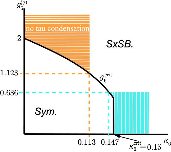
(a)       $\delta=1\,,R_{6}^{-1}=10\,\text{TeV}$ (b)       $\delta=1\,,R_{6}^{-1}=1\,\text{TeV}$

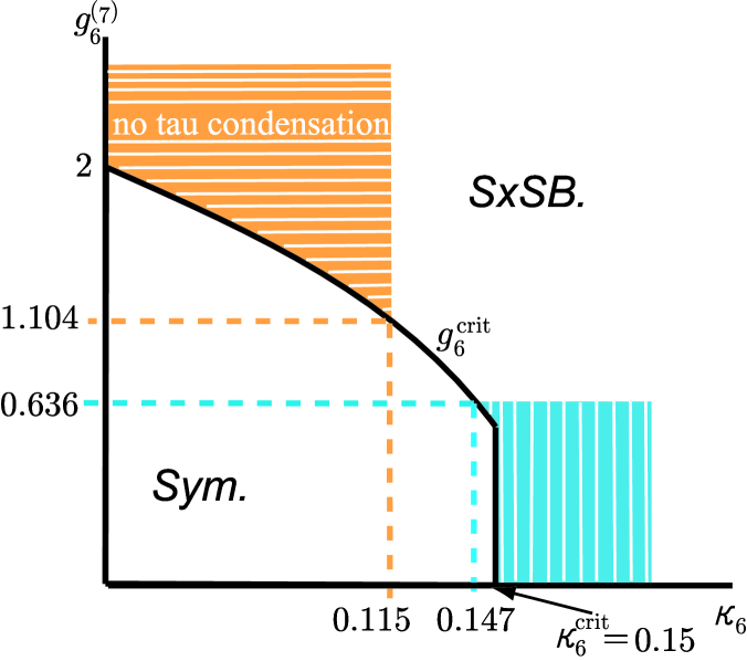
Figure 2: The phase diagram of D(=6)-dimensional gauged NJL model Gusynin:2004jp with the induced four-fermion coupling by the 7-dimensional bulk gluons (one compactified dimension $\delta=1$). The critical line in Eq.(72) is denoted by $g_{6}^{\rm crit}$ with the nonlocal gauge estimation. The region above $g_{6}^{\rm crit}$ is the $S\chi SB$-phase, and that below is the $Symmetric$-phase. The vertical stripe pattern regions are from Eq. (83): $g_{6}^{\rm crit}(\kappa_{t})<g_{6}^{\rm induced}<0.636$ or equivalently $\kappa_{t}>\kappa^{\rm crit}>\kappa_{6}^{\rm crit}(0.636)=0.147$. The horizontal stripe pattern regions are those satisfying Eq.(79), namely the region for the top condensate without tau condensation: (a) is for $R_{6}^{-1}=10\,\text{TeV}$ with $(\kappa_{t}(\Lambda_{\tau}),\,g_{6}^{\rm crit}(\kappa_{t}(\Lambda_{\tau})))=(0.113,\,1.123)$ and (b) is for $R_{6}^{-1}=1\,\text{TeV}$ with $(\kappa_{t}(\Lambda_{\tau}),\,g_{6}^{\rm crit}(\kappa_{t}(\Lambda_{\tau})))=(0.115,\,1.104)$. The tMAC scale satisfying Eq.(80) would be the overlap region between regions of the vertical and the horizontal stripe pattern, which does not exist in either case (a) or (b).

$8D\to 6D$-case

We now demonstrate that the tMAC scale does exist when the gluons in the 8-dimensional bulk give the induced four-fermion interactions in Eqs. (68), (69) (vertical stripe pattern regions Fig. 3):

$$0<g_{6}^{\rm induced}=g_{6}^{(8)}<1.22 (\text{by the lowest KK-mode}),$$

$$0.18<g_{6}^{\rm induced}=g_{6}^{(8)}<1.42 (\text{by the 4-th KK-modes}).$$ (85)

This implies :

$$\kappa_{t}(\Lambda_{\rm tM})>\kappa^{\rm crit}>\kappa_{6}(g_{6})\Big{|}_{g_{6}=1.22}=0.10 (\text{the lowest KK-mode}),$$

$$\kappa_{t}(\Lambda_{\rm tM})>\kappa^{\rm crit}>\kappa_{6}(g_{6})\Big{|}_{g_{6}=1.42}=0.08 (\text{sum to the 4-th KK-modes}).$$ (86)

From Fig. 1 or Fig. 4 we can see that this is fulfilled for

$$\Lambda_{\rm tM}>\begin{cases}10.2R_{6}^{-1}&\hskip 5.69054pt(\text{lowest only})\\[8.53581pt] 7.8R_{6}^{-1}&\hskip 5.69054pt(\text{sum to the 4-th}),\end{cases}$$ (87)

for $R_{6}^{-1}=10\,\text{TeV}$and

$$\Lambda_{\rm tM}>\begin{cases}10.3R_{6}^{-1}&\hskip 5.69054pt(\text{lowest only})\\[8.53581pt] 7.5R_{6}^{-1}&\hskip 5.69054pt(\text{sum to the 4-th}),\end{cases}$$ (88)

for $R_{6}^{-1}=1\,\text{TeV}$. Then this time there is an overlap with the scale required by the no tau condensation, Eq.(78):

$$\Lambda_{\rm tM}<\Lambda_{\tau}=\begin{cases}10.8R_{6}^{-1}&(\text{for}\,R_{6}^{-1}=10\,\text{TeV})\\[8.53581pt] 11.0R_{6}^{-1}&(\text{for}\,R_{6}^{-1}=1\,\text{TeV}).\end{cases}$$ (89)

Thus the tMAC scale does exist:

$$\Lambda_{\rm tM}R_{6}=\begin{cases}10.2-10.8&\hskip 5.69054pt(\text{lowest only})\\[8.53581pt] 7.8-10.8&\hskip 5.69054pt(\text{sum to the 4-th}),\end{cases}$$ (90)

for $R_{6}^{-1}=10\,\text{TeV}$ and

$$\Lambda_{\rm tM}R_{6}=\begin{cases}10.3-11.0&\hskip 5.69054pt(\text{lowest only})\\[8.53581pt] 7.5-11.0&\hskip 5.69054pt(\text{sum to the 4-th}),\end{cases}$$ (91)

for $R_{6}^{-1}=1\,\text{TeV}$.

As an illustration we show in Fig. 3 the region of Eq.(86) and Eq.(79) by the vertical stripe pattern region and by the horizontal stripe pattern region, respectively for $R_{6}^{-1}=10\,{\rm TeV}$ (A similar result is obtained for $R_{6}^{-1}=1\,{\rm TeV}$). The tMAC scale defined by Eq.(80) is the overlap region of these two, which does exist for the case of the induced four-fermion coupling $g_{6}^{(8)}$. In Fig. 4 we indicate the tMAC scale, Eq.(80), as the shaded region which is the overlap region of Eq.(86) and Eq.(79) for $R_{6}^{-1}=10\,{\rm TeV}$ and $R_{6}^{-1}=1\,{\rm TeV}$. Thus we conclude that tMAC scale does exist.

As to the concrete value of the tMAC scale, there is some ambiguity. Without knowing further information on the recoil effects of the brane, we may make a best compromise by taking a conservative estimate of the sum of the KK modes of the bulk gluons up till the 4th KK modes, which is quite stable against summing more KK modes contributions in a naive way (see Appendix A). Then our conservative estimate of the tMAC scale is

$$\Lambda_{\rm tM}R_{6}=\begin{cases}7.8-10.8&\hskip 5.69054pt(R_{6}^{-1}=10\,\text{TeV})\\[8.53581pt] 7.5-11.0&\hskip 5.69054pt(R_{6}^{-1}=1\,\text{TeV}).\end{cases}$$ (92)

Note however that we have a freedom of tuning the brane position to reduce the induced four-fermion interaction at our disposal, so that we can always adjust the tMAC scale to the high end of the above estimate:

$$\Lambda_{\rm tM}R_{6}=\begin{cases}10.8&\hskip 5.69054pt(R_{6}^{-1}=10\,\text{TeV})\\[8.53581pt] 11.0&\hskip 5.69054pt(R_{6}^{-1}=1\,\text{TeV}).\end{cases}$$ (93)

.

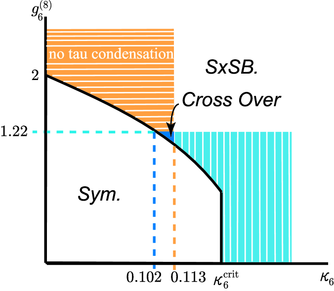
(a) (b)

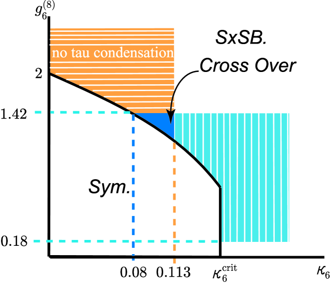
Figure 3: The phase diagram and the tMAC region by the nonlocal gauge fixing method; These figures are for $R_{6}^{-1}=10\,\text{TeV}$case. (a) is estimated by the lowest KK-mode only, and (b) is by the summation till the 4-th KK-modes. The vertical dashed lines are the value of $\kappa_{t}$ at scale $\Lambda_{\tau}$. The vertical stripe pattern regions are the allowed regions from Eq.(68), (69). In order to make top quark condense, these vertical stripe region and the horizontal stripe (no tau condensation) regions must have a cross over regions. In this figure, there exist cross over regions (shaded regions).

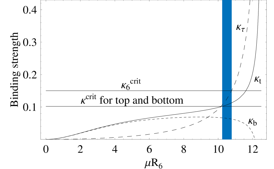
(a)        $R_{6}^{-1}=10\,\text{TeV}$, lowest (b)        $R_{6}^{-1}=10\,\text{TeV}$, 4-th

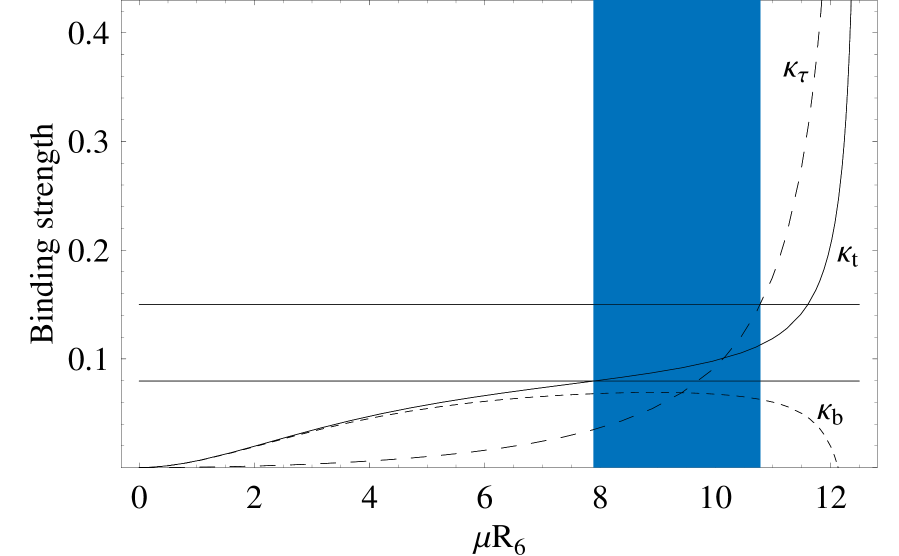
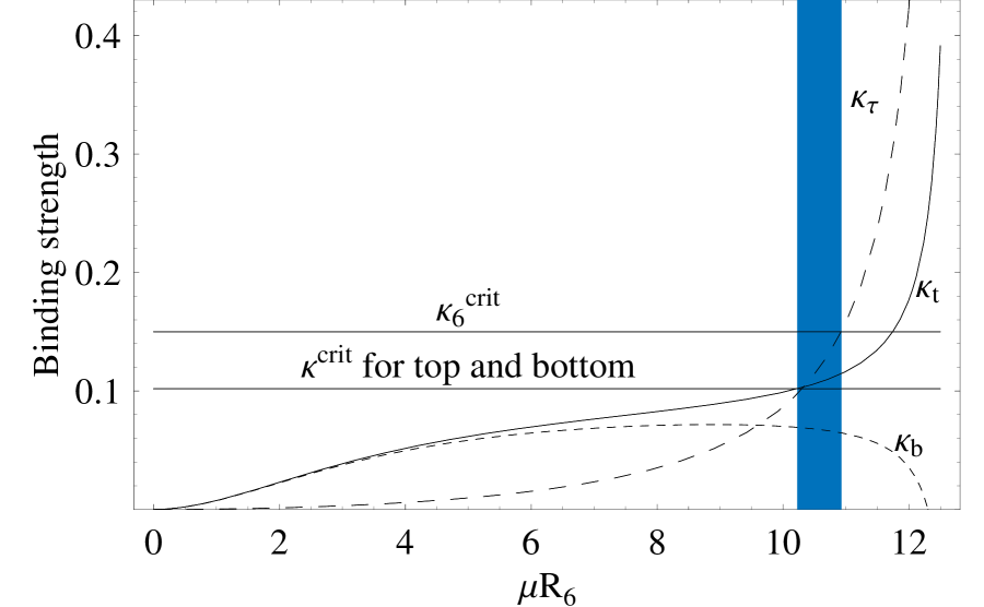
(c)        $R_{6}^{-1}=1\,\text{TeV}$, lowest (d)        $R_{6}^{-1}=1\,\text{TeV}$, 4-th

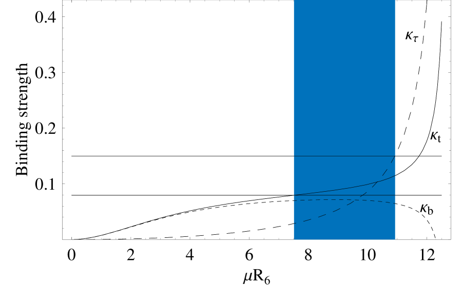
Figure 4: Binding strengths for tau, bottom and top. In (a) and (b) shown are the binding strengths $\kappa_{\tau},\kappa_{t}$ and $\kappa_{b}$ for tau, top and bottom, respectively on the 5-brane with $R_{6}^{-1}=10\,\text{TeV}$, while in (c) and (d) shown are those with $R_{6}^{-1}=1\,\text{TeV}$. The upper horizontal line in the figures is the critical binding strength for tau, $\kappa_{6}^{\rm crit}=0.15$ (nonlocal gauge fixing method). The lower line is the one for top and bottom, $\kappa^{\rm crit}$ derived by using the upper bound of $c$ (the coefficient of the dimensionless four fermion coupling) : (a),(c) are those by the lowest KK-mode only, while (b),(d) are those by the summation till the 4-th KK-modes. The shaded regions which are equivalent to the corresponding shaded regions in Fig. 3 are the tMAC scales: $\Lambda_{\rm tM}R_{6}={\rm(a)}10.2-10.8\,,{\rm(b)}7.8-10.8\,,{\rm(c)}10.3-11\,{\rm and}\,{\rm(d)}7.5-11$.

V Predictions of $m_{t}$ and $m_{H}$

We now calculate masses of the top quark $m_{t}$ and the Higgs boson $m_{H}$. Since it is rather complicated to do the numerical analysis of the TMSM with extra dimensions using the method of the original MTY MTY89 in 4 dimensions based on the SD equation and the Pagels-Stokar formula, we here follow the procedure of ACDH ACDH:2000hv (see also Kobakhidze:1999ce ) and Ref. HTY2003 where the 6-dimensional TMSM was rewritten into the form of the 6-dimensional SM with the compositeness condition á la Bardeen-Hill-Lindner (BHL) BHL:1989ds , which was then analyzed in the truncated KK effective theory by the renormalization group equations (RGEs) for top-yukawa coupling $y_{t}$ and Higgs quartic coupling $\lambda_{H}$ with the compositeness condition.

In Refs. ACDH:2000hv ; HTY2003 which have no explicit four-fermion interactions in 6 dimensions, the meaning of the compositeness condition was rather obscure. In contrast, in our case having explicit four-fermion interaction we can formulate straightforwardly the compositeness condition in the 6-dimensional TMSM in precisely the same manner as in the BHL for the 4-dimensional model. Note that the compositeness scale $\Lambda$, which is the scale of the induced four-fermion interactions, namely the compactification scale of the seven-th and eighth dimensions $\Lambda=R^{\rm-1}\equiv R_{7}^{\rm-1}=R_{8}^{\rm-1}$, is not an arbitrary parameter in contrast to ACDH ACDH:2000hv and Ref.Kobakhidze:1999ce but is identified with the tMAC scale, $\Lambda=\Lambda_{\rm tM}$ as in Ref. HTY2003 . Then the compositeness conditions read

$$y_{t}(\mu)\to\infty,\quad\frac{\lambda_{H}(\mu)}{y_{t}(\mu)^{4}}\to 0\quad(\mu\to\Lambda=\Lambda_{\rm tM})\,,$$ (94)

where $R^{-1}_{6}\leq\mu\leq\Lambda=R^{-1}=\Lambda_{\rm tM}$.

In the truncated KK effective theory the RGEs for the gauge couplings are Eq.(4) and Eq.(5) with Eqs.(6),(7), (8). Similarly, the RGEs for $y_{t}$ and $\lambda_{H}$ are given by

$$(4\pi)^{2}\mu\frac{dy_{t}}{d\mu}=\beta_{y_{t}}^{\rm SM}+\beta_{y_{t}}^{\rm KK}$$ (95)

$$(4\pi)^{2}\mu\frac{d\lambda_{H}}{d\mu}=\beta_{\lambda_{H}}^{\rm SM}+\beta_{\lambda_{H}}^{\rm KK},$$ (96)

where,

$$\beta_{y_{t}}^{\rm SM} = y_{t}\left[\,\left(3+\frac{3}{2}\right)y_{t}^{2}-8g_{3}^{2}-\frac{9}{4}g_{2}^{2}-\frac{17}{12}g_{Y}^{2}\,\right],$$ (97)

$$\beta_{y_{t}}^{\rm KK} = \left(6N_{\rm KK}^{f}+\frac{3}{2}N_{\rm KK}^{h}\right)\,y_{t}^{3}$$ (98)

$$\quad-N_{\rm KK}^{g}\left(8g_{3}^{2}+\frac{9}{4}g_{2}^{2}+\frac{17}{12}g_{Y}^{2}\right)\,y_{t}$$

$$\quad-\delta N_{\rm KK}^{gs}\left(\frac{4}{3}g_{3}^{2}-\frac{3}{8}g_{2}^{2}-\frac{1}{72}g_{Y}^{2}\right)\,y_{t},$$

$$\beta_{\lambda_{H}}^{\rm SM} = 12\left(\lambda_{H}y_{t}^{2}-y_{t}^{4}\right)+12\lambda_{H}^{2}$$ (99)

$$\quad+\frac{3}{4}(3g_{2}^{4}+2g_{2}^{2}g_{Y}^{2}+g_{Y}^{4})$$

$$\quad-3(3g_{2}^{2}+g_{Y}^{2})\lambda_{H},$$

$$\beta_{\lambda_{H}}^{\rm KK} = 24N_{\rm KK}^{f}\left(\lambda_{H}y_{t}^{2}-y_{t}^{4}\right)+12N_{\rm KK}^{h}\lambda_{H}^{2}$$ (100)

$$+N_{\rm KK}^{g}\left[\,\frac{3}{4}\left(3g_{2}^{4}+2g_{2}^{2}g_{Y}^{2}+g_{Y}^{4}\right)-3(3g_{2}^{2}+g_{Y}^{2})\lambda_{H}\,\right]$$

$$+\frac{\delta}{4}N_{\rm KK}^{gs}(3g_{2}^{4}+2g_{2}^{2}g_{Y}^{2}+g_{Y}^{4}).$$

By solving these RGEs with inputs Eq.(12) and the compositeness condition Eq. (94), we determine the running of $y_{t}(\mu)$ and $\lambda_{H}(\mu)$ and predict $m_{t}$ and $m_{H}$ by the condition:

$$m_{t}=v\,\frac{y_{t}(m_{t})}{\sqrt{2}},\quad m_{H}=v\,\sqrt{\lambda_{H}(m_{H})},$$ (101)

where $v=246\,\text{GeV}$.

We now present our main result: From the analysis in Sec. IV we predict $m_{t}$ and $m_{H}$ for the conservative estimate of $\Lambda_{\rm tM}$ in Eq.(92):

$$m_{t} = 178-187\,\text{GeV},$$

$$m_{H} = 183-199\,\text{GeV},$$ (102)

for $\Lambda_{\rm tM}=(7.8-10.8)\,R^{-1}_{6}\,(R^{-1}_{6}=10\text{TeV})$ , and

$$m_{t}=177-187\,\text{GeV},$$

$$m_{H}=186-207\,\text{GeV},$$ (103)

for $\Lambda_{\rm tM}=(7.5-11.0)\,R^{-1}_{6}\,(R^{-1}_{6}=1\,\text{TeV})$.

It is remarkable that our top mass prediction

$$m_{t}=177-187\,{\rm GeV}\quad(R_{6}^{-1}=1-10\,{\rm TeV}).$$ (104)

is quite stable against changing the compactification scale of the 5-th and 6-th dimensions $R^{-1}_{6}$. This $m_{t}$ is consistent with the new experimental value (pole mass) CDF/D0:2004 , $178.0\pm 4.3\,{\rm GeV}$, and the corresponding $\overline{\rm MS}$-mass, $m_{t}^{\overline{\rm MS}}=169.8\pm 4.1\,{\rm GeV}$, obtained through a formula Marciano:1989xd .

As to the Higgs mass prediction, our conservative estimate implies

$$m_{H}=183-207\,{\rm GeV}\quad(R_{6}^{-1}=1-10\,{\rm TeV}).$$ (105)

This Higgs boson mass prediction, somewhat similar to that of Ref. HTY2003 , $m_{H}=176-188$ GeV, is characteristically smaller than that of the typical dynamical EWSB models like technicolor. On the other hand, the value is substantially larger than that of typical supersymmetric models, $m_{H}\mathop{<}\limits_{\displaystyle{\sim}}130$ GeV (MSSM) or $m_{H}\mathop{<}\limits_{\displaystyle{\sim}}150$ GeV (NMSSM). Thus the present scenario is clearly distinguished from many of the typical models beyond the SM, either dynamical or SUSY models, simply through the Higgs mass observation. The Higgs boson of this mass range decays into weak boson pair almost 100%. It will be immediately discovered in $H\to WW^{(*)}/ZZ^{(*)}$ once the LHC starts.

Some comments are in order:

As we discussed in Sec.III, there is a possibility that the recoil effects of the brane reduce higher KK modes drastically, in which case only the lowest KK-mode contribution, instead of sum up till the 4th KK modes, may be the relevant contribution to the induced four-fermion coupling $g_{6}^{\rm induced}$. If we take the $\Lambda_{\rm tMAC}$ values for only the lowest KK-mode as given in Eqs.(90) and (91) instead of the conservative estimate of $\Lambda_{\rm tM}$ in Eq.(92), the prediction is:

$$m_{t}=178-180\,\text{GeV},\hskip 11.38109ptm_{H}=183-186\,\text{GeV}$$ (106)

for $\Lambda_{\rm tM}=10.2-10.8\,R^{-1}_{6}\,(R^{-1}_{6}=10\,\text{TeV})$ ,

$$m_{t}=177-179\,\text{GeV},\hskip 11.38109ptm_{H}=186-190\,\text{GeV}$$ (107)

for $\Lambda_{\rm tM}=10.3-11.0\,R^{-1}_{6}(R^{-1}_{6}=1\,\text{TeV})$. The prediction becomes somewhat more restricted for the mass range.

If we further exploited the freedom of the brane position as to tune the induced four-fermion coupling as given by Eq. (93), then we may pinpoint the prediction to the lower end values in Eqs.(102),(103),(106) and (107):

$$m_{t}=177-178\,\text{GeV}\quad(R^{-1}_{6}=1-10\,\,\text{TeV}),$$ (108)

$$m_{H}=183-186\,\text{GeV}\quad(R^{-1}_{6}=1-10\,\,\text{TeV}).$$ (109)

Note that the above lower end values of the prediction are not altered even if we included 20% errors of the possible ambiguity of the SD equation we mentioned earlier. Considering the top mass prediction should be close to the reality, the most plausible value of the Higgs mass prediction in our model would be such lower end values Eq.(109).

For comparison, we may present values calculated when our analysis is performed in the Landau gauge fixing as in Ref. HTY2003 , although the Landau gauge analysis is less reliable than that in the nonlocal gauge as we discussed before. The result actually is not changed so much: The tMAC scale is

$$\Lambda_{\rm tM}R_{6}=\begin{cases}8.3-10.5&\hskip 5.69054pt(\text{lowest only})\\[8.53581pt] 6.5-10.5&\hskip 5.69054pt(\text{sum till the 4-th}),\end{cases}$$ (110)

for $R_{6}^{-1}=10\,\text{TeV}$ and

$$\Lambda_{\rm tM}R_{6}=\begin{cases}8.0-10.6&\hskip 5.69054pt(\text{lowest only})\\[8.53581pt] 6.5-10.6&\hskip 5.69054pt(\text{sum till the 4-th}),\end{cases}$$ (111)

for $R_{6}^{-1}=1\,\text{TeV}$. Note that the lower end value for the sum till the 4-th KK modes is the same for $R_{6}^{-1}=10\,\text{TeV}$ and $R_{6}^{-1}=1\,\text{TeV}$, which is determined by the requirement of no bottom condensation since in this case the $\kappa^{\rm crit}$ is lower than that in the nonlocal gauge (the value given in Fig.4). Accordingly, the masses for top and Higgs are predicted as

$$m_{t}=179-192\,\text{GeV},\hskip 11.38109ptm_{H}=187-211\,\text{GeV}$$ (112)

for $\Lambda_{\rm tM}=6.5-10.8\,R^{-1}_{6}\,(R^{-1}_{6}=10\,\text{TeV})$, and

$$m_{t}=178-192\,\text{GeV},\hskip 11.38109ptm_{H}=187-218\,\text{GeV}$$ (113)

for $\Lambda_{\rm tM}=6.5-11.0\,R^{-1}_{6}\,(R^{-1}_{6}=1\,\text{TeV})$, which are compared with Eq.(102) and (103), respectively.

VI Summary

We have proposed a version of the Top Mode Standard Model (TMSM) in six dimensions (5-brane in the eight-dimensional bulk), with the third generation quarks/leptons and the $SU(2)_{L}\times U(1)$ gauge bosons living on the 5-brane with the 5-th and 6-th dimensions compactified on $T^{2}/Z_{2}$ with TeV scale, $R_{5}^{-1}=R_{6}^{-1}=1-10\,\text{TeV}$, while the $SU(3)$ gluons, living in the eight-dimensional bulk with the 6-th and 7-th dimensions compactified on $T^{2}/Z_{2}$ with yet higher scale, $R_{7}^{-1}=R_{8}^{-1}=\Lambda\gg R_{6}^{-1}$, give rise to induced four-fermion interactions of top and bottom (but not of tau) on the 5-brane. The first and second generations are living in four dimensions. Having such a four-fermion interactions induced by the bulk gluon KK modes in addition to the Standard Model gauge interactions on the 5-brane, the model for top/bottom takes the form of the 6-dimensional gauged NJL model whose critical line is given by Eq.(72) with $D=6$. We have shown that such an induced four-fermion coupling is well above the critical line $g_{6}^{\rm induced}=g_{6}^{(8)}>1/2$, and in fact strong enough as to trigger the top condensate without bottom and tau condensates. Namely, there exists an energy region $\mu$ (tMAC scale) satisfying the condition Eq.(80), see the shaded region in Figs. 3 and 4.

Here we note that our estimation of the induced four-fermion interactions crucially depends on the existence of UVFP HTY:2000uk ; Agashe:2000nk ; Kazakov:2002jd ; Dienes:2002bg . Although existence of such a UVFP is still in controversy, pro and con, in lattice studies kawai and other nonperturbative methods Gies:2003ic , its existence will result in resolving a possible conflict with arguments of the perturbative unitarity Chivukula:2003kq which presume no such a UVFP. Moreover, the brane fluctuation strongly suppresses higher KK modes as in Eq.(65) Bando:1999 , which makes the “divergence” of the summation of KK modes merely superficial. This is another source to avoid conflict with the perturbative unitarity arguments. We also note that as was explicitly checked in Ref.HTY2003 the KK modes summation is fairly independent of the truncation scheme for $D=6$ and $D=8$, though not for $D=10$.

In the truncated KK effective theory DDG we employed in this paper, the $SU(3)\times SU(2)\times U(1)_{Y}$ SM gauge couplings on the 5-brane are “strong” enough to trigger the top quark condensate but still “weak” enough not to destroy the perturbative picture completely: The binding strength is given by $\kappa_{i}=\cal{O}$$(0.1)$ $(i=t,b,\tau)$ for the relevant energy region $\mu R_{6}<10$ (see Fig. 4), which are much smaller than the naive dimensional analysis $\kappa=\cal{O}$$(1)$. Thus the gauge theory (including $U(1)$) on the 5-brane also is not obviously in conflict with the perturbative unitarity.

It should be emphasized that our compactification of the 8-dimensional bulk into the 5-brane, $D=8\rightarrow D=6$, is on $T^{2}/Z_{2}$ instead of $T^{2}$, which leaves us with parameters, the brane position $x_{70},\,x_{80}$, to tune the four-fermion coupling close to the critical line so that the dynamical mass of the top quark, which is otherwise on the order of cutoff $\Lambda$, can be kept on the weak scale order in the SD gap equation: $m_{t}\sim v=246\text{GeV}\ll\Lambda$. Such a freedom corresponds to tuning the VEV of the composite Higgs, $v\ll\Lambda$, in the BHL formulation based on the RGE’s plus compositeness conditions.

We then calculated based on the BHL formulation the predicted values:

$$m_{t}=178-187\,\text{GeV},\quad m_{H}=183-207\,\text{GeV}.$$ (114)

The top mass prediction is consistent with the experimental value (see the discussions below Eq. (104)). The Higgs boson mass prediction is a rather characteristically small value compared with those in other strongly coupled Higgs models like technicolor which are usually larger than that. On the other hand, the value is substantially larger than that of typical supersymmetric models, $m_{H}\mathop{<}\limits_{\displaystyle{\sim}}130$ GeV (MSSM) or $m_{H}\mathop{<}\limits_{\displaystyle{\sim}}150$ GeV (NMSSM). Thus the present scenario is clearly distinguished from many of the typical models beyond the SM simply through the Higgs mass observation. The Higgs boson of this mass range decays into weak boson pair almost 100% and will be immediately discovered in $H\to WW^{(*)}/ZZ^{(*)}$ once the LHC starts.

Several comments are in order:

• In this paper we discussed mass of the top quark as the origin of the masses of W and Z bosons and the composite Higgs. What about the mass of other quarks and leptons?

  • Bottom mass
    In the original TMSM MTY89 , the bottom mass must come from $G_{ts}$-term in Eq. (1) ($G^{(2)}$ term in Ref.MTY89 ) :

    $$G_{tb}\left(\epsilon^{ik}\epsilon_{jl}\bar{\psi}_{L}^{i}{\psi_{R}}_{j}\bar{\psi}_{L}^{k}{\psi_{R}}_{l}\right)+h.c.,$$ (115)

    which explicitly breaks the Peccei-Quinn symmetry and yields $m_{b}=-G_{tb}\langle\bar{t}t\rangle$ after the top condensation takes place. Were it not for the $G_{ts}$ term, the bottom condensate due to strong $G_{b}$ term in Eq.(1) would lead to the visible axion (2nd paper in Ref.MTY89 ) which is already ruled out. As was emphasized in Ref.Tanabashi:1989sz the $G_{ts}$ term does not arise from the massive vector meson exchange model and hence from the gauge interaction. However it was pointed out Yamawaki:1990ue that the instanton effects can give rise to such a term, although it turned out very small in the original TMSM with large cutoff Tanabashi:1992rn . It was argued Hill:1994hp ; He:2001fz , however, in the topcolor scenario with much smaller cutoff scale compared with the original TMSM, that such instanton effects can produce a reasonable amount of mass for the bottom.

    In the case at hand, we may naively guess from the $D=4$ color instanton that the bulk gluon instanton living in $D=8$ bulk would give the $D=6$ $G_{ts}$-like four-fermion interaction on the 5-brane, although little is known about the higher dimensional instantons (see e.g., Ref. Hill:2000rr ).

  • Tau mass
    In the original TMSM MTY89 , the tau mass also comes from a term similar to the $G_{ts}$ term with the $\psi=(t,b)$ replaced by $\psi=(\nu_{\tau},\tau^{-})$ for the one pair of $\bar{\psi}_{L}\psi_{R}$. In the present model, however, without introducing ad hoc four-fermion interactions, we would need some larger picture such as the Pati-Salam gauge unification between bottom and tau.

  • 1st and 2nd generation masses
    There are various possible ways to communicate the top condensate with the mass operator of the 1st and 2nd generations: The simplest one would be the one similar to the extended technicolor (ETC)Dimopoulos:1979es with the role of the technifermion now replaced by the top quark, namely through the horizontal gauge interaction on the 3-brane. Since the anomalous dimension of the top quark condensate of our model in terms of the 4-dimensional language is close to 2, $\gamma_{m}\simeq 2$ MTY89 ; Yamawaki96 , much larger than even the walking technicolor ($\gamma_{m}\simeq 1$) Yamawaki:1985zg , there is no such conflict to the Flavor-Changing Neutral Currents (FCNC) as that in the ETC.

• Constraints from the precision experiments
  The new particles other than the SM particles contributing to the $S$ parameter are KK modes of the top/bottom which , however, are vector-like and hence yield little contributions to the $S$ parameter Maekawa:1994yd . As to the $T$ parameter or $\Delta\rho$, the summation of KK modes below the cutoff $\Lambda$ contributes to $\Delta\rho$ as $\Delta\rho\sim 10(M_{W}R)^{2}$ Nath:1999fs which would unfavor the lower $R^{-1}\sim 1{\rm TeV}$ similarly to the previous model with $D=8$ HTY2003 .

• UV sensitivity
  Our model is based on the dynamics of 6-dimensional gauged NJL model, but when $N_{c}=3,N_{f}=2$, the 6-dimensional gauged NJL model is non-renormalizable even in the nonperturbative sense discussed in Ref. Gusynin:2004jp . We would need a better-controlled theory beyond $\Lambda$.

• In this paper, the freedom of the position of the 5-brane in the higher dimensional bulk played a central role for consistency in our model. The origin of this degree of freedom remains to be investigated in the brane dynamics.

Appendix A The possibility of the fermion condensation on the 3-brane

We here consider whether or not the fermion fixed on the 3-brane can condense by the four-fermion interactions induced by the bulk gluons in $D(<4)$ dimensions. We consider the case with $(D-4)$-compactification on $T^{\delta}/Z_{2}^{k}(\delta\equiv D-4,k=1,2,\cdots)$ of the extra dimensions, with the compactification radii $R_{5}=R_{6}=R$, in which the only gluon propagates. If the KK-modes effects of the bulk gluons give rise to four-fermion interactions on the 3-brane, such four-fermion interactions may take the form:

$$\begin{split}\mathcal{L}_{\rm 4F}&=\frac{1}{2}\cdot\frac{2^{k}}{(3\pi R)^{\delta}}\cdot\frac{g_{3}^{2}(M_{1})}{2M_{1}^{2}}\cdot c_{4}^{(D)}\times(\bar{\psi}\psi)^{2}\\ &=\frac{G_{4}^{(D)}}{2N_{c}}(\bar{\psi}\psi)^{2}\end{split}$$ (116)

where $M_{1}$ is the mass of the lowest KK-mode $M_{1}=R^{-1}$ and $g_{3}$ is the QCD coupling on the 3-brane, and $c_{4}^{(D)}$ is the dimensionless coefficients to be estimated below. The dimensionless four-fermion coupling on the 3-brane is thus

$$\begin{split}g_{4}^{(D)}&=2^{2}G_{4}^{(D)}M_{1}^{2}\Omega_{\rm NDA}\\ &=2^{2}\cdot\frac{2N_{c}}{2}\frac{2^{k}}{(3\pi R)^{\delta}}\frac{g_{3}^{2}(M_{1})}{2M_{1}^{2}}c_{4}^{(D)}\cdot M_{1}^{2}\Omega_{\rm NDA}\\ &=c_{4}^{(D)}\cdot 2^{(4/2-1)}N_{c}\cdot g_{3}(M_{1})^{2}\Omega_{\rm NDA}.\end{split}$$ (117)

Let us estimate of $c_{4}^{(D)}$ for $D=6,8$ cases.

Case.1 : $D=6$ cases

First, we consider the $T^{2}/Z_{2}$-compactification. Imposing periodic boundary condition:

$$\begin{split}G_{\mu}(x,x_{5},x_{6})&=G_{\mu}(x,x_{5}+2\pi R,x_{6})\\ &=G_{\mu}(x,x_{5},x_{6}+2\pi R),\end{split}$$ (118)

and a $Z_{2}$ condition:

$$G_{\mu}(x,x_{5},x_{6})=G_{\mu}(x,-x_{5},-x_{6}),$$ (119)

we decompose $G_{\mu}$ as

$$G_{\mu}(x,x_{5},x_{6})=\frac{1}{2\pi R}\Bigl{[}G_{\mu,00}(x)+\sqrt{2}\sum_{[n]_{1}}^{N_{\rm KK}}\tilde{G}_{\mu}^{[1]}+2\sum_{[n]_{2}}^{N_{\rm KK}}\tilde{G}_{\mu}^{[2]}\Bigl{]},$$ (120)

where

$$\tilde{G}_{\mu}^{[1]} = G_{\mu,c0}^{[n]_{1}}\cos\frac{n_{1}x_{5}}{R}+G_{\mu,0c}^{[n]_{1}}\cos\frac{n_{1}x_{6}}{R}$$ (121)

$$\tilde{G}_{\mu}^{[2]} = G_{\mu,cc}^{[n]_{2}}\cos\frac{n_{1}x_{5}}{R}\cos\frac{n_{2}x_{6}}{R}+G_{\mu,ss}^{[n]_{2}}\sin\frac{n_{1}x_{5}}{R}\sin\frac{n_{2}x_{6}}{R}.$$ (122)

We are interested in the upper bound for $g_{4}^{(6)}$, which is realized at $x_{5}=x_{6}=0$ where these KK-mode induce a four-fermion interaction on the 3-brane as:

$$\mathcal{L}_{\rm 4F} = \frac{1}{2}\frac{2}{(2\pi R)^{2}}\Biggl{[}\sum_{[n]_{1}}\frac{g_{6,3}^{2}(M_{[n]_{1}})}{2M_{[n]_{1}}^{2}}\times 2$$ (123)

$$\hskip 56.9055pt+2\sum_{[n]_{2}}\frac{g_{6,3}^{2}(M_{[n]_{2}})}{2M_{[n]_{2}}^{2}}\times D_{[n]_{2}}\Biggr{]}(\bar{\psi}\psi)^{2}$$

$$= \frac{1}{2}\frac{2}{(2\pi R)^{2}}\Biggl{[}\sum_{[n]_{1}}\frac{g_{6,3}^{2}(M_{1})}{2M_{1}^{2}}\cdot\Bigl{(}\frac{M_{1}}{M_{[n]_{1}}}\Bigr{)}^{4}\times 2$$

$$\hskip 56.9055pt+2\sum_{[n]_{2}}\frac{g_{6,3}^{2}(M_{1})}{2M_{1}^{2}}\cdot\Bigl{(}\frac{M_{1}}{M_{[n]_{2}}}\Bigr{)}^{4}\times D_{[n_{2}]}\Biggr{]}(\bar{\psi}\psi)^{2}$$

$$= \frac{1}{2}\frac{g_{3}^{2}(M_{1})}{2M_{1}^{2}}\times c_{4}^{(6,k=1)}\times(\bar{\psi}\psi)^{2},$$

where $D_{[n]_{i}}$ is the degeneracy having the same $N$ for each $[n]_{i}$,

$$[n]_{1}\equiv[n_{1}],\quad[n]_{2}\equiv[n_{1},n_{2}],\cdots,$$ (124)

and $M_{[n]_{1}}\,,\,M_{[n]_{2}}$ are

$$M_{[n]_{1}}^{2}=n^{2}M_{1}^{2},\quad M_{[n]_{2}}^{2}=(n_{1}^{2}+n_{2}^{2})M_{1}^{2},\cdots.$$ (125)

We used the fact that the dimensionless bulk QCD coupling $\hat{g}_{6,3}$ is nearly on the UVFP, i.e.,

$$\hat{g}_{6,3}^{2}(M_{[n]_{i}})=g_{6,3}^{2}(M_{1})\Bigl{(}\frac{M_{1}}{M_{[n]_{1}}}\Bigr{)}^{2},$$ (126)

and

$$g_{6,3}^{2}(M_{1})=\frac{(2\pi R)^{2}}{2}g_{3}^{2}(M_{1}).$$ (127)

From the above we read the coefficient $c_{4}^{(6,k=1)}$ as

$$c_{4}^{(6,k=1)}=2\sum_{[n]_{1}}\Bigl{(}\frac{M_{1}}{M_{[n]_{1}}}\Bigr{)}^{4}+2\sum_{[n]_{2}}D_{[n]_{2}}\Bigl{(}\frac{M_{1}}{M_{[n]_{2}}}\Bigr{)}^{4},$$ (128)

which yields the dimensionless four-fermion-coupling $g_{4}^{(6,k=1)}$ (Eq. (117)):

$$g_{4}^{(6,k=1)}=c_{4}^{(6,k=1)}\cdot 2^{2}N_{c}\cdot g_{3}(M_{1})^{2}\Omega_{\rm NDA}.$$ (129)

Note that the summation in Eq. (120) stands for the summation of KK-mode whose $\text{mass}^{2}$ is

$$M_{[n]_{i}}^{2}=\sum_{k}^{i}\frac{n_{k}^{2}}{R^{2}}=\frac{N}{R^{2}}\leq\frac{N_{\rm KK}}{R^{2}}.$$ (130)

Next, we consider $T^{2}$-compactification ($k=0$), i.e. we impose the periodic boundary condition Eq. (118) only. In this case, the result is independent of the brane position so that we take $x_{5}=x_{6}=0$. In this case we must consider $n_{1}=\pm 1,\pm 2,\cdots,$ etc , for $c_{4}^{(6,k=0)}$ and $c_{4}^{(6,k=0)}$ is given by

$$c_{4}^{(6,k=0)}=2^{2}\sum_{[n]_{1}}\Bigl{(}\frac{M_{1}}{M_{[n]_{1}}}\Bigr{)}^{4}+2^{3}\sum_{[n]_{2}}D_{[n]_{2}}\Bigl{(}\frac{M_{1}}{M_{[n]_{2}}}\Bigr{)}^{4},$$ (131)

which yields

$$g_{4}^{(6,k=0)}=c_{4}^{(6,k=0)}\cdot 2^{2}N_{c}\cdot g_{3}(M_{1})^{2}\Omega_{\rm NDA}.$$ (132)

The numerical estimate of $g_{4}^{(6,k=0)}$ with $c_{4}^{(6,k=1)},\,c_{4}^{(6,k=0)}$ in Case.1 is shown Fig. 5(a). We calculated $g_{4}^{(6)}$ till $N_{\rm KK}=200$ concretely in this figure. From this figure, we conclude that the bulk gluons do not give rise to the S$\chi$SB-phase for the fermions on the 3-brane.

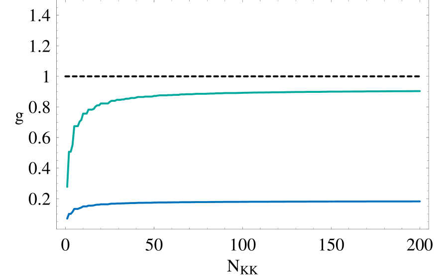
(a)        $\delta=2$ case (b)        $\delta=4$ case

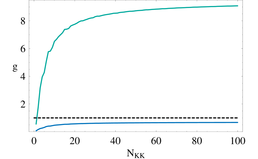
Figure 5: The dimensionless four fermion coupling: $g_{4}^{(6)}$ on the 3-brane summing up till $N_{\rm KK}$; The horizontal dashed line is $g_{4}^{\rm crit}=1$ on the 3-brane. Fig. (a) is for $D=6(\delta=2)$, and (b) for $D=8(\delta=4)$. The upper lines are $T^{\delta}$-compactification cases with $k=0$ and the lower lines are $T^{\delta}/Z_{2}^{k}$-compactification cases with $k=1$(for $\delta=2$) and $k=2$(for $\delta=4$).

Case.2 : $D=8$ cases

As in Case.1, the imposed boundary condition for $T^{4}/Z_{2}^{2}$-compactification case is also a periodic boundary condition:

$$\begin{split}G_{\mu}(x,y,z)&=G_{\mu}(x,y+2\pi R,z)\\ &=G_{\mu}(x,y,z+2\pi R),\end{split}$$ (133)

and the $Z_{2}^{2}$ condition:

$$G_{\mu}(x,y,z) = G_{\mu}(x,-y,z)$$ (134)

$$= G_{\mu}(x,y,-z),$$

where $y=x_{5,6}$ and $z=x_{7,8}$. Making a short-hand notation of the $G_{\mu,c000}^{[n]_{1}}\cos(n_{1}x_{5}/R)$ as $G_{\mu,c000}$, etc. we write the KK-decomposition of $G_{\mu}(x,y,z)$ as:

$$G_{\mu}(x,y,z)=\frac{1}{(2\pi R)^{2}}\Bigl{[}G_{\mu,0000}(x)+\sqrt{2}\sum_{[n]_{1}}^{N_{\rm KK}}\tilde{G}_{\mu}^{[1]}+2\sum_{[n]_{2}}^{N_{\rm KK}}\tilde{G}_{\mu}^{[2]}+2\sqrt{2}\sum_{[n]_{3}}^{N_{\rm KK}}\tilde{G}_{\mu}^{[3]}+4\sum_{[n]_{4}}^{N_{\rm KK}}\tilde{G}_{\mu}^{[4]}\Bigl{]},$$ (135)

where

$$\tilde{G}_{\mu}^{[1]} = G_{\mu,c000}^{[n]_{1}}+G_{\mu,s000}^{[n]_{1}}+G_{\mu,0c00}^{[n]_{1}}+G_{\mu,0s00}^{[n]_{1}}$$ (136)

$$\hskip 11.38109pt+G_{\mu,00c0}^{[n]_{1}}+G_{\mu,00s0}^{[n]_{1}}+G_{\mu,000c}^{[n]_{1}}+G_{\mu,000s}^{[n]_{1}},$$

$$\tilde{G}_{\mu}^{[2]} = G_{\mu,cc00}^{[n]_{2}}+G_{\mu,c0c0}^{[n]_{2}}+G_{\mu,c00c}^{[n]_{2}}+G_{\mu,0cc0}^{[n]_{2}}$$ (137)

$$\hskip 11.38109pt+G_{\mu,0c0c}^{[n]_{2}}+G_{\mu,00cc}^{[n]_{2}}+G_{\mu,ss00}^{[n]_{2}}+G_{\mu,00ss}^{[n]_{2}},$$

$$\tilde{G}_{\mu}^{[3]} = G_{\mu,ccc0}^{[n]_{3}}+G_{\mu,cc0c}^{[n]_{3}}+G_{\mu,c0cc}^{[n]_{3}}+G_{\mu,0ccc}^{[n]_{3}}$$ (138)

$$\hskip 11.38109pt+G_{\mu,ssc0}^{[n]_{3}}+G_{\mu,ss0c}^{[n]_{3}}+G_{\mu,c0ss}^{[n]_{3}}+G_{\mu,0css}^{[n]_{3}}$$

$$\tilde{G}_{\mu}^{[4]} = G_{\mu,cccc}^{[n]_{4}}+G_{\mu,ccss}^{[n]_{4}}+G_{\mu,sscc}^{[n]_{4}}+G_{\mu,ssss}^{[n]_{4}}.$$ (139)

Our interest is an estimation of the upper bound for four-fermion coupling, which is realized at the brane positions $x_{50}=x_{60}=x_{70}=x_{80}=0$ where we rewrite these gluons KK-modes effects into the four-fermion interactions on the 3-brane:

$$\mathcal{L}_{\rm 4F} = \frac{1}{2}\frac{2^{2}}{(2\pi R)^{4}}\Biggl{[}\sum_{[n]_{1}}\frac{g_{8,3}^{2}(M_{[n]_{1}})}{2M_{[n]_{1}}^{2}}\times 4+2\sum_{[n]_{2}}\frac{g_{8,3}^{2}(M_{[n]_{2}})}{2M_{[n]_{2}}^{2}}\times 6\times D_{[n]_{2}}$$ (140)

$$\hskip 56.9055pt+2^{2}\sum_{[n]_{3}}\frac{g_{8,3}^{2}(M_{[n]_{3}})}{2M_{[n]_{3}}^{2}}\times 4\times D_{[n]_{3}}+2^{3}\sum_{[n]_{4}}\frac{g_{8,3}^{2}(M_{[n]_{4}})}{2M_{[n]_{4}}^{2}}\times D_{[n]_{4}}\Biggr{]}(\bar{\psi}\psi)^{2}$$

$$= \frac{1}{2}\frac{2^{2}}{(2\pi R)^{4}}\Biggl{[}\sum_{[n]_{1}}\frac{g_{8,3}^{2}(M_{[n]_{1}})}{2M_{1}^{2}}\cdot\Bigl{(}\frac{M_{1}}{M_{[n]_{1}}}\Bigr{)}^{6}\times 4+2\sum_{[n]_{2}}\frac{g_{8,3}^{2}(M_{[n]_{2}})}{2M_{[n]_{2}}^{2}}\cdot\Bigl{(}\frac{M_{1}}{M_{[n]_{2}}}\Bigr{)}^{6}\times 6\times D_{[n]_{2}}$$

$$\hskip 71.13188pt+2^{2}\sum_{[n]_{3}}\frac{g_{8,3}^{2}(M_{[n]_{3}})}{2M_{[n]_{3}}^{2}}\cdot\Bigl{(}\frac{M_{1}}{M_{[n]_{3}}}\Bigr{)}^{6}\times 4\times D_{[n]_{3}}+2^{3}\sum_{[n]_{4}}\frac{g_{8,3}^{2}(M_{[n]_{4}})}{2M_{[n]_{4}}^{2}}\cdot\Bigl{(}\frac{M_{1}}{M_{[n]_{4}}}\Bigr{)}^{6}\times D_{[n]_{4}}\Biggr{]}(\bar{\psi}\psi)^{2}$$

$$= \frac{1}{2}\frac{g_{3}^{2}(M_{[n]_{1}})}{2M_{1}^{2}}\times c_{4}^{(8,k=2)}\times(\bar{\psi}\psi)^{2}.$$

We have used that the dimensionless bulk gauge coupling $\hat{g}_{8,3}$ is nearly on the UVFP, i.e.,

$$\hat{g}_{8,3}^{2}(M_{[n]_{i}})=g_{8,3}^{2}(M_{1})\Bigl{(}\frac{M_{1}}{M_{[n]_{1}}}\Bigr{)}^{4},$$ (141)

and that

$$g_{8,3}^{2}(M_{1})=\frac{(2\pi R)^{4}}{2^{2}}g_{3}^{2}(M_{1}).$$ (142)

Then the dimensionless four-fermion coupling $g_{4}^{(8,k=2)}$ (Eq. (117)) is given by

$$g_{4}^{(8,k=2)}=c_{4}^{(8,k=2)}\cdot 2^{2}N_{c}\cdot g_{3}(M_{1})^{2}\Omega_{\rm NDA},$$ (143)

where $c_{4}^{(8,k=2)}$ is

$$c_{4}^{(6,k=1)} = 4\sum_{[n]_{1}}\Bigl{(}\frac{M_{1}}{M_{[n]_{1}}}\Bigr{)}^{6}+12\sum_{[n]_{2}}D_{[n]_{2}}\Bigl{(}\frac{M_{1}}{M_{[n]_{2}}}\Bigr{)}^{6}$$ (144)

$$+16\sum_{[n]_{3}}D_{[n]_{3}}\Bigl{(}\frac{M_{1}}{M_{[n]_{3}}}\Bigr{)}^{6}$$

$$+8\sum_{[n]_{4}}D_{[n]_{4}}\Bigl{(}\frac{M_{1}}{M_{[n]_{4}}}\Bigr{)}^{6}.$$

Next, we consider $T^{4}$-compactification case ($k=0$). As in the $T^{2}$-case in Case.1, the brane position does not matter and we take $x_{5}=x_{6}=x_{7}=x_{8}=0$:

$$c_{4}^{(8,k=0)} = 4\times 2\sum_{[n]_{1}}\Bigl{(}\frac{M_{1}}{M_{[n]_{1}}}\Bigr{)}^{6}+6\times 2^{2}\sum_{[n]_{2}}D_{[n]_{2}}\Bigl{(}\frac{M_{1}}{M_{[n]_{2}}}\Bigr{)}^{6}$$ (145)

$$+8\times 2^{3}\sum_{[n]_{3}}D_{[n]_{3}}\Bigl{(}\frac{M_{1}}{M_{[n]_{3}}}\Bigr{)}^{6}$$

$$+4\times 2^{4}\sum_{[n]_{4}}D_{[n]_{4}}\Bigl{(}\frac{M_{1}}{M_{[n]_{4}}}\Bigr{)}^{6},$$

which yields

$$g_{4}^{(8,k=0)}=c_{4}^{(8,k=0)}\cdot 2^{2}N_{c}\cdot g_{3}(M_{1})^{2}\Omega_{\rm NDA}.$$ (146)

The resultant $g_{4}$ with $c_{4}^{(8,k=2)},\,c_{4}^{(8,k=0)}$ in Case.2 is shown in Fig. 5(b). We calculated $g_{4}$ till $N_{\rm KK}=100$ in this figure. In $T^{4}$-compactification case, the fermions on the 3-brane can condense which is consistent with Ref. Dobrescu:1998dg ; Abe:2002 , while for $T^{4}/Z_{2}^{2}$-case the $g_{4}$ is almost unchanged with respect to increasing $N_{\rm KK}$ and $g_{4}$ is always less than $g_{4}^{\rm crit}$ for a cutoff for the extra dimensions. That is, in Fig. 5(b) we can read $g_{4}^{(8)}$ as

$$g_{4}^{(8)}(N_{\rm KK}=100)<g_{4}^{\rm crit}=1,$$ (147)

and hence the fermions fixed on the 3-brane do not condense by the induced four-fermion interactions due to the bulk gluons with $T^{4}/Z_{2}^{2}$-compactified extra dimension.

Appendix B KK modes sum for $G^{(8)}_{6}$

We here estimate the summation of the induced four-fermion coupling $G^{(8)}_{6}$ in Eq.(61) or its dimensionless coupling $g^{(8)}_{6}$ in Eq.(62). As we discussed in the text, sum of infinite KK modes would give us a divergent result and the anomalous dimension of the induced four-fermion operators may make the higher KK mode contributions even more enhanced. But the recoil effects give us an exponential damping factor in Eq.(65) and should make the sum finite Bando:1999 . Due to ignorance of the precise parameters of the exponential damping factor at this moment, we here ignore both the anomalous dimension effects and the recoil effects altogether and simply sum up finite number of KK modes numerically with understanding that the sum should be finite.

In the $8D\to 6D$ case, our imposing boundary conditions are ($X=x_{\mu},x_{5},x_{6}$)

$$G_{M}(X,x_{7},x_{8}) = G_{M}(X,x_{7}+2\pi R_{7},x_{8})$$

$$= G_{M}(X,x_{7},x_{8}+2\pi R_{8}),$$

$$G_{M}(X,x_{7},x_{8}) = G_{M}(X,-x_{7},-x_{8}).$$ (149)

The decomposition of the bulk gluons $G_{M}$ with $R_{7}=R_{8}=R=\Lambda^{-1}$ is given by

$$\begin{split}G_{M}(X,x_{7},x_{8})=\frac{1}{2\pi R}\Biggl{[}G_{M,00}(X)&+\sqrt{2}\sum_{n=1}^{N_{\rm KK}}G^{[n]}_{M,c0}(X)\cos\frac{nx_{7}}{R}\\ &+\sqrt{2}\sum_{n=1}^{N_{\rm KK}}G^{[n]}_{M,0c}(X)\cos\frac{nx_{8}}{R}\\ &+2\sum_{n_{1},n_{2}=1}^{N_{\rm KK}}G^{[n_{1},n_{2}]}_{M,cc}(X)\cos\frac{n_{1}x_{7}}{\Lambda^{-1}}\cos\frac{n_{2}x_{8}}{R}\\ &+2\sum_{n_{1},n_{2}=1}^{N_{\rm KK}}G^{[n_{1},n_{2}]}_{M,ss}(X)\sin\frac{n_{1}x_{7}}{\Lambda^{-1}}\sin\frac{n_{2}x_{8}}{R}\Biggr{]}.\end{split}$$ (150)

In order to esitmate the upper bound for $g_{6}^{(8)}$, we calculate for $(x_{70},x_{80})=(0,0)$ only. In consequence, we have

$$\mathcal{L}_{\rm 4F} = \frac{3}{4}\cdot\frac{1}{2}\cdot\frac{2}{(2\pi R)^{2}}\Biggl{[}\sum_{[n]_{1}}\frac{g_{8,3}^{2}(M_{[n]_{1}})}{2M_{[n]_{1}}^{2}}\times 2$$

$$\hskip 56.9055pt+2\sum_{[n]_{2}}\frac{g_{6,3}^{2}(M_{[n]_{2}})}{2M_{[n]_{2}}^{2}}\times D_{[n]_{2}}\Biggr{]}(\bar{\psi}\psi)^{2}$$

$$= \frac{1}{2}\frac{g_{3}^{2}(M_{1})}{2M_{1}^{2}}\times c_{6}^{(8)}(0,0)\times(\bar{\psi}\psi)^{2}.$$

$D_{[n]_{i}}$ is the number of degeneracy, that is the combinations of $(n_{1},n_{3},\cdots)$ having the same KK-gluons masses: $M_{[n]_{i}}(M^{2}_{[n]_{i}}=(n_{1}^{2}+n_{2}^{2}+\cdots)M_{1}^{2})$ where $M_{1}=\Lambda$.

Next, we have used the fact that dimensionless bulk gauge coupling $\hat{g}^{2}_{8,3}$ is approximately near the UVFP and set

$$g_{8,3}^{2}(n\Lambda)=\frac{g_{8,3}^{2}(\Lambda)}{n^{4}}.$$ (152)

Thus considering $g^{2}_{6,3}(\Lambda)\equiv 2g^{2}_{8,3}(\Lambda)/{(2\pi R)^{2}}$, we get the total coefficient of four-fermion operator

$$c_{6}^{(8)}(0,0)=2\sum_{[n]_{1}}\Bigl{(}\frac{M_{1}}{M_{[n]_{1}}}\Bigr{)}^{6}+2\sum_{[n]_{2}}D_{[n]_{2}}\Bigl{(}\frac{M_{1}}{M_{[n]_{2}}}\Bigr{)}^{6},$$ (153)

Hence the bound of the dimensionless induced four-fermion coupling defined in Eq.(41) is given by

$$g_{6}^{(8)} = c_{6}^{(8)}(x_{70},x_{80})\cdot 2^{2}N_{c}\cdot\hat{g}_{6*,3}^{2}\Omega_{\rm NDA}=c_{6}^{(8)}(x_{70},x_{80})\cdot 2^{2}N_{c}\cdot\frac{3}{44}$$ (154)

$$= c_{6}^{(8)}(x_{70},x_{80})\cdot\frac{3N_{c}}{11}$$

$$\leq c_{6}^{(8)}(0,0)\cdot\frac{3N_{c}}{11}$$ (155)

where we again used $\hat{g}_{6,3}^{2}\Omega_{\rm NDA}=\hat{g}_{6*,3}^{2}\Omega_{\rm NDA}=3/44$.

The numerical calculation result for the upper bound of $g_{6}^{(8)}$ (sum by $N_{\rm KK}=100$) is shown in Fig. 6, that is, we get the upper bound of $g_{6}^{(8)}$:

$$g_{6}^{(8)}\lesssim 1.42.$$ (156)

Since this upper bound is nearly the same as the one in Eq. (67), the sum till the 4th KK modes, we may conclude that all KK-modes effects contributions are well approximated by the first few KK-modes effects contributions. If we consider recoil effects more seriously, the main contribution may even be the lowest KK-mode only.

Figure 6: The estimation of $g^{(8)}_{6}$ for Eq. (61) for the summation by $N_{\rm KK}$(KK-mode $\text{mass}^{2}$ is $N_{\rm KK}^{2}M_{1}^{2}$)

References

(1)
H. Fukano and K. Yamawaki, in Proc. 2004 International Workshop on Dynamical
Symmetry Breaking (DSB 04), Dec. 21-22, 2004, Nagoya University, Nagoya, ed. by M. Harada
and K. Yamawaki (Nagoya University, 2005) p. 115-124.
(2)
V. A. Miransky, M. Tanabashi, and K. Yamawaki,
Phys. Lett. B 221, 177 (1989);
Mod. Phys. Lett. A 4, 1043 (1989).
(3)
K.-I. Kondo, H. Mino, and K. Yamawaki,
Phys. Rev. D39, 2430 (1989);
K. Yamawaki,
in Proc. Johns Hopkins Workshop on Current Problems in Particle
Theory 12, Baltimore, June 8-10, 1988,
edited by G. Domokos and S. Kovesi-Domokos
(World Scientific Pub. Co. , Singapore 1988).
(4)
T. Appelquist, M. Soldate, T. Takeuchi, and L. C. R. Wijewardhana,
in Proc. Johns Hopkins Workshop on Current Problems in Particle
Theory 12, Baltimore, June 8-10, 1988,
edited by G. Domokos and S. Kovesi-Domokos
(World Scientific Pub. Co. , Singapore 1988).
(5)
Y. Nambu, Enrico Fermi Institute Report No. 89-08, 1989.
(6)
W. J. Marciano, Phys. Rev. Lett. 62, 2793 (1989);
Phys. Rev. D41, 219 (1990).
(7)
H. Pagels, and S. Stokar,
Phys. Rev. D20, 2947 (1979).
(8)
W. A. Bardeen, C. T. Hill and M. Lindner,
Phys. Rev. D41, 1647 (1990).
(9)
K. Yamawaki,
in Proceedings of 14th Symposium on Theoretical Physics
“Dynamical Symmetry Breaking and Effective Field Theory”,
Cheju Island, Korea, July 21-26, 1995, ed. J. E. Kim
(Minumsa Pub. Co., Korea, 1996) p.43-86,
[arXiv:hep-ph/9603293].
(10)
V. A. Miransky, Dynamical Symmetry Breaking
in Quantum Field Theories (World Scientific Pub. Co., Singapore 1993).
(11)
C. T. Hill, and E. H. Simmons,
Phys. Rept. 381, 235 (2003),
[Erratum ibid.390, 553 (2004)].
(12)
K.-I. Kondo, M. Tanabashi and K. Yamawaki,
in Proc. 1989 Workshop on Dynamical Symmetry Breaking, Nagoya,
1989, eds. T. Muta and K. Yamawaki (Nagoya University, 1990) p. 28-36.
(13)
C. T. Hill,
Phys. Lett. B 266, 419 (1991).
(14)
B. A. Dobrescu and C. T. Hill,
Phys. Rev. Lett. 81, 2634 (1998);
R. S. Chivukula, B. A. Dobrescu, H. Georgi and C. T. Hill,
Phys. Rev. D59, 075003 (1999).
(15)
H. J. He, C. T. Hill and T. M. P. Tait,
Phys. Rev. D 65, 055006 (2002).
(16)
N. Maekawa,
Prog. Theor. Phys. 93, 919 (1995);
Phys. Rev. D 52, 1684 (1995).
(17)
B. A. Dobrescu, Phys. Lett. B461, 99 (1999).
(18)
H. C. Cheng, B. A. Dobrescu, and C. T. Hill,
Nucl. Phys. B589, 249 (2000).
(19)
M. Hashimoto and D. K. Hong,
Phys. Rev. D 71, 056004 (2005).
(20)
N. Arkani-Hamed, H. C. Cheng, B. A. Dobrescu and L. J. Hall,
Phys. Rev. D62, 096006 (2000),
(21)
M. Hashimoto, M. Tanabashi and K. Yamawaki,
Phys. Rev. D64, 056003 (2001).
(22)
V. Gusynin, M. Hashimoto, M. Tanabashi, and K. Yamawaki,
Phys. Rev. D65, 116008 (2002).
(23)
K. R. Dienes, E. Dudas and T. Gherghetta,
Phys. Lett. B436, 55 (1998);
Nucl. Phys. B537, 47 (1999);
I. Antoniadis, S. Dimopoulos, A. Pomarol and M. Quiros,
Nucl. Phys. B544, 503 (1999);
Z. Kakushadze,
Nucl. Phys. B548, 205 (1999).
(24)
N. Rius and V. Sanz,
Phys. Rev. D 64, 075006 (2001);
H. Abe, K. Fukazawa, and T. Inagaki,
Prog. Theor. Phys. 107, 1047 (2002).
(25)
M. Hashimoto, M. Tanabashi and K. Yamawaki,
Phys. Rev. D69, 076004 (2004).
(26)
V. P. Gusynin, M. Hashimoto, M. Tanabashi and K. Yamawaki,
Phys. Rev. D 70, 096005 (2004).
(27)
S. Eidelman et al.[Particle Data Group Collaboration],
Phys. Lett. B592, 1 (2004).
(28)
K. Agashe,
JHEP 0105, 017 (2001).
(29)
D. I. Kazakov,
JHEP 0303, 020 (2003)
(30)
K. R. Dienes, E. Dudas and T. Gherghetta,
Phys. Rev. Lett. 91, 061601 (2003).
(31)
S. Raby, S. Dimopoulos and L. Susskind,
Nucl. Phys. B169, 373 (1980).
(32)
T. Kugo and M. G. Mitchard,
Phys. Lett. B 282, 162 (1992).
(33)
M. Bando, T. Kugo, T. Noguchi and K. Yoshioka,
Phys. Rev. Lett. 83, 3601 (1999).
(34)
T. Appelquist, K. D. Lane and U. Mahanta,
Phys. Rev. Lett. 61, 1553 (1988).
(35)
A. B. Kobakhidze,
Phys. Atom. Nucl. 64, 941 (2001),
[Yad. Fiz. 64, 1010 (2001)],
(36)
CDF Collaboration and D0 Collaboration and Tevatron Electroweak Working Group (P. Azzi et al.),
[arXiv:hep-ex/0404010].
(37)
[CDF Collaboration],
arXiv:hep-ex/0507006.
(38)
t. T. E. Group [the D0 Collaboration],
arXiv:hep-ex/0507091.
(39)
W. J. Marciano,
Phys. Rev. Lett. 62, 2793 (1989).
(40)
H. Kawai, M. Nio, and Y. Okamoto,
Prog. Theor. Phys. 88, 341 (1992);
S. Ejiri, J. Kubo, and M. Murata,
Phys. Rev. D62, 105025 (2000);
K. Farakos, P. de Forcrand, C. P. Korthals Altes, M. Laine,
and M. Vettorazzo,
Nucl. Phys. B655, 170 (2003).
(41)
H. Gies,
Phys. Rev. D 68, 085015 (2003);
T. R. Morris,
JHEP 0501, 002 (2005)
(42)
R. S. Chivukula, D. A. Dicus, H. J. He and S. Nandi,
Phys. Lett. B 562, 109 (2003).
(43)
K. Yamawaki,
DPNU-90-42,
in Proc. 1990 International Workshop on Strong Coupling Gauge
Theories and Beyond, July 28-31, 1990, Nagoya, eds.
T. Muta and K. Yamawaki
(World Scientific Pub. Co., Singapore, 1991) p.13-36.
(44)
M. Tanabashi,
DPNU-92-03,
in Proc. International Workshop on Electroweak Symmetry Breaking, Hiroshima, Nov 12-15, 1991, eds. W.A. Bardeen, J. Kodaira and T. Muta (World Scientific Pub. Co., Singapore, 1992) p. 75-91;
T. Elliott and S. F. King,
Z. Phys. C 58, 609 (1993).
(45)
C. T. Hill,
Phys. Lett. B 345, 483 (1995).
(46)
C. T. Hill and P. Ramond,
Nucl. Phys. B 596, 243 (2001).
(47)
S. Dimopoulos and L. Susskind,
Nucl. Phys. B 155, 237 (1979);
E. Eichten and K. D. Lane,
Phys. Lett. B 90, 125 (1980).
(48)
B. Holdom,
Phys. Lett. B 150, 301 (1985);
K. Yamawaki, M. Bando and K. Matumoto,
Phys. Rev. Lett. 56, 1335 (1986);
T. Akiba and T. Yanagida,
Phys. Lett. B 169, 432 (1986);
T.W. Appelquist, D. Karabali and L.C.R. Wijewardhana,
Phys. Rev. Lett. 57, 957 (1986)
;
M. Bando, T. Morozumi, H. So and K. Yamawaki,
Phys. Rev. Lett. 59, 389 (1987).
(49)
P. Nath and M. Yamaguchi,
Phys. Rev. D60, 116004 (1999).
(50)
H. Abe and T. Inagaki,
Phys. Rev. D66, 085001 (2002).
(b)
(b)
(b)
(b)
(b)
(b)
(b) , 4-th
(d) , 4-th
(b) case