Deconfinement transition dynamics and early thermalization in QGP

Abstract

We perform SU(3) Lattice Gauge Theory simulations of the deconfinement transition attempting to mimic conditions encountered in heavy ion collisions. Specifically, we perform a sudden temperature quench across the deconfinement temperature, and follow the response of the system in successive simulation sweeps under spatial lattice expansion and temperature fall-off. In measurements of the Polyakov loop and structure functions a robust strong signal of global instability response is observed through the exponential growth of low momentum modes. Development of these long range modes isotropizes the system which reaches thermalization shortly afterwards, and enters a stage of quasi-equilibrium expansion and cooling till its return to the confinement phase. The time scale characterizing full growth of the long range modes is largely unaffected by the conditions of spatial expansion and temperature variation in the system, and is much shorter than the scale set by the interval to return to the confinement phase. The wide separation of these two scales is such that it naturally results in isotropization times well inside 1 fm/c.

I Introduction

Recent heavy ion collision experiments at RHIC have produced a wealth of data on hadron spectra and their anisotropies, in particular the magnitudes of radial and elliptical flows. This data reveals, perhaps unexpectedly, coherence in particle production and strong collective flow phenomena. It turns out that about 99% of the single hadron data ($p_{T}<1.5$ GeV) are very well described by the hydrodynamics of a near-perfect fluid, provided the initial condition of very rapid thermalization (in $\sim 0.5fm/c$) is introduced Heinz:2004pj - Kolb:2003dz . This strongly indicates that the quark-gluon plasma (QGP) formed at RHIC energies is a strongly coupled fluid.

At asymptotically high temperatures above the deconfinement $T_{c}$, where the running coupling $g(T)$ is small, QCD is well-described as a gas of weakly coupled quasi-particles, and has been much studied by perturbative techniques. At the energy densities achieved in the high energy heavy ion collisions, however, perturbative treatment of the equilibration process appears not to be applicable. Various estimates of thermalization times based on perturbative scattering processes have been obtained, e.g. in the so called parton-cascade approach to the time evolution of hard partons, or the bottom-up scenario MG , BjV , BMSS incorporating saturation picture (see Kar , IV for review) initial conditions. They all result into thermalization times much longer than those needed by the hydrodynamical simulations. It has been argued that this is a generic feature of any dynamical evolution based only on perturbative scattering processes Kov .

Even within a weak coupling analysis, however, non-perturbative effects may contribute to the dynamics. It has been pointed out that, in a plasma with an anisotropic hard parton distribution, instabilities may develop in soft gauge field modes generated within the linear response approximation ALM - H . It has been argued that these small-amplitude unstable modes are not stabilized by (non-Abelian) non-linearities; and thus can grow to amplitudes large enough to contribute $O(1)$ fraction to the total energy density, and drive isotropization of the hard modes faster than any hard collision equilibration time scale ALMY .

Various investigations of the evolution of these semiclassical instabilities have been carried out probing beyond the linear regime, and, in particular, within the hard-loop effective action Rebh1 - Rebh2 . They generally indicate that such instabilities indeed persist when non-Abelian non-linearities are taken into account within the weak coupling regime. At some point, however, other non-perturbative dynamics at strong effective couplings defined at scales appropriate to the nonlinear interaction of such growing long range modes must enter. Still, consideration of such potential instabilities properly point to a basic underlying question which should be addressed from a more general point of view.

When systems are driven far from equilibrium by sudden changes in external conditions, the approach to a new equilibrium state involves, in general, complex nonequilibrium processes. Such situations arise, for example, in a ‘quench’ to the metastable region across a first-order transition boundary, or from a one-phase region to the multiphase coexistence region across a second-order transition. The study of the dynamics of such far-from-equilibrium processes is still at an early stage of development. Nonetheless, from many studies, mostly in condensed matter physics systems, two broad classes of responses have been roughly identified.

Immediately after a rapid quench, the state of the system, as characterized by the appropriate order parameter, is nearly identical to the state before. The fields must then find some way to adjust toward values appropriate to the conditions after the quench. One way the system may decay towards equilibrium is by the excitation of finite amplitude localized fluctuations that may grow or coalesce as in nucleation, or interact in other ways over time. This typically indicates that the system finds itself in some sort of metastable state. Another way is by the immediate development of a spatially modulated order parameter whose amplitude grows continuously from zero throughout the sample. Spinodal decomposition is a prime example of this type of response, and the term is often used loosely to generically denote such globally unstable behavior. It should be pointed out that the boundary between these two rough classes is not sharp in all cases.

At RHIC heavy-ion collisions in the central rapidity region achieve the sudden deposition of energy densities reaching $\sim 30GeV/fm^{3}$. The first most basic question that must be posed then is: which general type of dynamic response is characteristic of a rapid transition across the confinement-deconfinement boundary in QCD? In the case of heavy-ion collisions, the question must be further qualified by the inclusion of the effects of rapid expansion and temperature variation, as well as finite volume. This is the issue we explore in this paper.

To get some intuition, we first investigate this question briefly within an effective action approach in Section 2. Indeed, much of the current understanding of the early time evolution of systems out of equilibrium has been obtained by investigating classes of stochastic equations that are natural dynamical (time dependent) generalizations of the Landau-Ginzburg (LG) effective action models of the static (equilibrium) theory (gunton:1985 , Chaikin:1997 ). In the case of the confinement - deconfinement transition, the relevant order parameter is the Polyakov loop (Wilson line), and LG effective actions for it have been considered in Pisarski:2000eq - HKW . Corresponding dynamical model generalizations can then be used to examine the question posed above. We consider the predictions of such a model briefly in Section 2 below.

Though the effective model approach often proves valuable, what is ultimately needed is an ab initio treatment in the full nonperturbative formulation of the exact theory, i.e. lattice gauge theory. Unfortunately, there is no established simulation formalism for directly extracting physical properties in non-equilibrium real-time evolution in quantum field theory. What one can do, however, is mimic Minkowski real-time dynamics by Glauber stochastic dynamics evolution. Thus starting with the system in thermalized equilibrium, one performs a temperature quench and follows the system, over successive simulation sweeps, on its path toward regaining equilibrium. Though this cannot be directly identified with the exact real-time evolution, it is known from many studies, mostly of condensed matter systems, to accurately reflect it. At the very least, the method provides a consistent picture of the basic features of the system’s real-time response. It has been extensively and successfully used for many systems exhibiting, in particular, first-order transitions. Indeed, in studies of binary alloys and binary fluids it has been found to reproduce the experimentally observed behavior in quantitative detail gunton:1983 . In the case of gauge theories, the method was first used in the pioneering studies in Miller:2000mr ; Miller:2000pd ; Miller:2001ym . More, recently, such studies of the dynamics of phase transitions in spin and gauge theory systems were undertaken and much extended in Bazavov:2004wc ; Berg:2003mn ; Berg:2003hc ; Berg:2004qb ; Velytsky:2002fn .

In this paper, building on these previous gauge theory studies, we consider $SU(3)$ gauge theory under conditions mimicking the situation encountered in heavy-ion collisions. This we do in Section 3 which constitutes the main part of the paper. Specifically, we examine the response after a sudden quench into the deconfinement phase under varying conditions of spatial expansion and temperature variation. In this first investigation, we consider only pure $SU(3)$ gauge theory, i.e. no quarks, as the deconfinement transition is driven by gluonic dynamics. In simulation measurements of structure functions and Polyakov loops, we follow the evolution of the system from the quench till its return to the confinement phase. The main outcome of our study is that two relevant, widely separated time scales emerge. First, a strong and robust signal of rapid growth of very long range modes is observed after the quench. Most importantly, the time scale of full development of these low momentum modes is essentially unaffected by the presence, over a wide range of parameters, of spatial expansion and temperature variation in the system. The development of these modes ‘isotropizes’ the system, which reaches full quasi-equilibrium shortly afterwards as signaled by the full decay of the structure function. It thus enters a stage of expansion and cooling, characterized by a second, much longer time scale, till its return to the confinement phase. The wide separation of these two scales accords well with what is seen in heavy-ion collision experiments. Having arrived at this robust qualitative picture, we also attempt to make a more quantitative comparison of what is seen in these simulations to hydrodynamical phenomenology (subsection 3.3). There are certainly uncertainties here, not least of which is the fact that we do not include fermions which can make a significant contribution especially at the late stage near the return to confinement. Still, one finds that the separation of scales is such that, for any reasonable choice of parameters, isotropization times well inside $1\ fm/c$ result naturally.

Finally, in Section 4 we briefly discuss our conclusions and directions for further work.

II Effective action models

Effective action models allow one to build simple theories of initial time evolution of systems driven out of equilibrium by a quench. Such theories can be build for general classes of models. A simple linear theory (Cahn-Hilliard) was first proposed for models of type B with conserved order parameter Cahn:1958 . The generalization to models of type A with non-conserved order parameters is straightforward, see, for example, Berg:2004qb ; Velytsky:2004 . For a general overview see e.g. gunton:1985 ; Chaikin:1997 .

Though such effective models are not our primary focus in this paper, it is useful to briefly consider them as they provide useful insight into the possible behavior of the system that can be checked against the outcome of simulations in the actual gauge theory. For $SU(3)$ gauge theory the low energy degrees of freedom are represented by Polyakov loops, and standard potential models for them are known and well studied Pisarski:2000eq ; W ; HKW . Adopting the potential for the Polyakov loop $l$ (a complex quantity) in Pisarski:2000eq

$${\mathcal{V}}(l)=\left(-\frac{b_{2}}{2}|l|^{2}-\frac{b_{3}}{6}(l^{3}+(l^{*})^{3})+\frac{1}{4}(|l|^{2})^{2}\right)b_{4}T^{4}\;,$$ (1)

the coupled set of Langevin equations is

$$\frac{\partial l}{\partial t}=-\Gamma\frac{\delta S}{\delta l^{*}}+\eta,\quad\mbox{and its}\quad c.c.$$ (2)

Here $S$ is the standard Landau-Ginzburg action

$$S=\int d^{3}x\left(\frac{1}{2}|\partial_{i}l|^{2}+{\mathcal{{V}}}(l)\right)\;,$$ (3)

$\Gamma$ is the response coefficient, which defines the relaxation time scale of the system, and $\eta$ is a noise term. We will ignore the noise term, since it can be shown that it does not affect the resulting rate of growth of fluctuations F1 .

We are interested in the fluctuations of the Polyakov loop $l$ around some average value $l_{0}$:

$$l(\vec{{r}},t)=l_{0}+u(\vec{{r}},t),$$ (4)

Using (1) and (2), the system of equations for the fluctuations is

$$\frac{\partial u}{\partial t}=-\Gamma\left[-\frac{1}{2}\nabla^{2}u+\left(c_{1}u+c_{2}u^{*}+c_{3}\right)\right]\quad\textnormal{and its}\quad c.c.\;,$$ (5)

where $c_{1}=(-b_{2}/2+|l_{0}|^{2})b_{4}T^{4}$, $c_{2}=(1/2l_{0}^{2}-b_{3}l_{0}^{*})b_{4}T^{4}$ and $c_{3}=(-b_{2}/2l_{0}-b_{3}/2l_{0}^{*2}+1/2l_{0}^{2}l_{0}^{*})b_{4}T^{4}$ are complex numbers. Note that $c_{1}=c_{1}^{*}$.

We solve for the Fourier transforms $u(\vec{{k}},t)$ and $v(\vec{{k}},t)$ of the fluctuations $u(\vec{{r}},t)$ and $u^{*}(r,t)$, respectively, which, from (5) satisfy:

$$\frac{\partial u(\vec{{k}},t)}{\partial t}+\Gamma\left[(\frac{1}{2}k^{2}+c_{1})u(k)+c_{2}v(k)\right] = c(k)$$

$$\frac{\partial v(\vec{{k}},t)}{\partial t}+\Gamma\left[(\frac{1}{2}k^{2}+c_{1}^{*})v(k)+c_{2}^{*}u(k)\right] = c^{*}(k)\;,$$ (6)

where $c(k)=c(-k)=-\Gamma c_{3}\sum_{\vec{{r}}}\exp(i\vec{{k}}\cdot\vec{{r}})$. Note also that $u^{*}(-\vec{{k}},t)=v(\vec{{k}},t)$. The non-zero modes are governed by the homogeneous part of these equations. Its eigenvalues are

$$\omega_{1,2}(k)=-\Gamma(\frac{1}{2}k^{2}+c_{1}\pm|c_{2}|),$$ (7)

and the eigenvectors are

$$S_{1,2}=\left(\begin{array}[]{c}\pm c_{2}/|c_{2}|\\ 1\end{array}\right).$$ (8)

The solution is

$$\left(\begin{array}[]{c}u(\vec{k},t)\\ v(\vec{k},t)\end{array}\right)=C_{1}S_{1}e^{\omega_{1}(k)t}+C_{2}S_{2}e^{\omega_{2}(k)t}.$$ (9)

Here, an analysis of modes similar to that of the real case (spin systems, $SU(2)$) (Bazavov:2004wc - Berg:2004qb ) can be applied. If $c_{1}\pm|c_{2}|<0$, one will observe exponential growth. Spinodal decomposition-like behavior then results if we have exponential growth in at least one exponent, i.e. when $c_{1}<|c_{2}|.$ The structure function (connected Polyakov 2-point function)

$$S(\vec{k},t)=\Bigg{<}u(\vec{k},t)\,v(-\vec{k},t)\Bigg{>}$$ (10)

follows similar behavior (Cf. Bazavov:2004wc ).

Next, we want to study the effect of spatial expansion. We work in new coordinates of rapidity $\eta=1/2\ln(t+z)/(t-z)$ and proper time $\tau$ :

$$t=\tau cosh(\eta)\;,\qquad z=\tau sinh(\eta).$$ (11)

Here we assume the $z$-axes to be the axes of expansion (collision). The change in the corresponding part of the Minkowski metric is $dt^{2}-dz^{2}=d\tau^{2}-\tau^{2}d\eta^{2}$, with the transverse coordinates left unchanged. Keeping the rapidity constant results in a constant rate of expansion in the system, the speed of expansion being proportional to the distance from the collision center: $v=z/t$, with $t$ the time after collision. In the new coordinates the metric is similar to the Robertson-Walker metric and is defined as $ds^{2}=g_{\mu\nu}dx_{\mu}dx_{\nu}=d\tau^{2}-a^{2}(\tau)d(\tau_{0}\eta)^{2}-dx_{\perp}^{2}$, i.e.

$$g_{\mu\nu}=\mbox{diag}\,\left(1,\;-1,\;-1,\;-a^{2}(\tau)\right)$$ (12)

where $a(\tau)=\tau/\tau_{0}$ is the ‘scale factor’, and $\tau_{0}$ is the parameter controlling the rate of expansion.

The obvious naive generalization of the model above is to substitute

$$\nabla^{2}\rightarrow g_{ij}\partial_{i}\partial_{j}$$

in the action (3), and to consider dynamics in the proper frame.

Eq. (2) now gives

$$\frac{\partial l}{\partial\tau}=-\Gamma\left[-\nabla_{\bot}^{2}l-a^{2}(\tau)\nabla_{\|}^{2}l+\frac{\partial V(l)}{\partial l}\right],\quad\mbox{and its}\quad c.c.\;,$$ (13)

where $\nabla_{\bot}^{2}=\partial_{x}^{2}+\partial_{y}^{2}$ and $\nabla_{\|}^{2}=\partial_{\eta}^{2}$. Going through the previous development amounts to the naive substitution $\vec{k}^{2}\rightarrow\vec{k}_{\perp}^{2}+a^{2}(\tau)k_{\|}^{2}$ in the eigenvalues:

$$\omega_{1,2}(k)=-\Gamma\left[\frac{1}{2}(\vec{k}_{\perp}^{2}+a^{2}(\tau)k_{\|}^{2})+c_{1}\pm|c_{2}|\right].$$ (14)

This now gives a growth of fluctuations governed by a 3rd order polynomial in $\tau$ in the exponent:

$$\left(\begin{array}[]{c}u(\vec{k},t)\\ v(\vec{k},t)\end{array}\right)=C_{1}S_{1}\exp\int_{0}^{\tau}\omega_{1}(\vec{k},\tau^{\prime})d\tau^{\prime}+C_{2}S_{2}\exp\int_{0}^{\tau}\omega_{2}(\vec{k},\tau^{\prime})d\tau^{\prime}.$$ (15)

Thus we observe that if

$$\frac{1}{2}(\vec{k}_{\perp}^{2}+a^{2}(\tau)k_{\|}^{2})<c_{1}-|c_{2}|\;,$$

there is an explosive growth, much faster than in the non-expanding case. Let us for simplicity consider only longitudinal modes. We see that the critical mode Chaikin:1997 is

$$k_{\parallel}^{c}=\frac{2}{a^{2}(\tau)}(c_{1}-|c_{2}|).$$ (16)

This is rather remarkable dynamics where the critical mode (and all modes at momentum scales below it) is moving in time. During initial time there are more scales involved but as time progresses only very large scale regions participate. The prediction of growth under expansion by a higher than linear power exponent is tested against the simulation results in the following section.

III Simulation study of deconfinement dynamics in $SU(3)$ LGT

In this section we present a numerical study of the effects of spatial expansion and varying temperature on the dynamical evolution following a sudden quench into the deconfined phase of the $SU(3)$ gauge theory on the lattice. We thus try to mimic conditions encountered in heavy-ion collisions. We use periodic boundary conditions, as we do not study the effects of finite size per se. A study of the role of the finiteness of the system would certainly be of interest, but is left for a future study. Also, in the customary heavy-ion collision picture the initial expansion is one-dimensional, becoming three-dimensional at later stages of the evolution Bjorken:1983 . Here, as we discuss further below, we simplify matters by considering a uniform expansion in all spatial directions. This is related to isotropic expansion in the proper frame at a fixed rapidity value. We first study the effect of such expansion; then we add the effect of varying temperature.

We use a field based heat bath update of the $SU(3)$ fields. To accelerate the dynamics there are 2 attempts to update the field per sweep. This is somewhat different from standard link-based updates; however, it is still in Glauber universality class. The time flow is proportional to the link-based heatbath with links visited in random order. Therefore, the peak values of the non expanding quench are slightly different from previous studies Bazavov:2004wc where a heat bath update is performed on links visited in systematic order.

We use a space-time anisotropic lattice in order to be able to independently control temperature and expansion. The anisotropic action is Karsch:1982ve

$$S=-\beta_{\xi}/3\sum_{x}\textrm{Re}\left[\xi^{-1}\sum_{i>j}\textrm{Tr}U_{x,ij}+\xi\sum_{i}\textrm{Tr}U_{x,0i}\right],$$ (17)

where $i$, $j$ runs over space-like directions, $\xi=a/a_{\tau}$ is the space-time anisotropy, $\beta_{\xi}=6/g_{\xi}^{2}$, and $g_{\xi}^{2}=g_{\sigma}\cdot g_{\tau}$ is the anisotropic coupling. Then, by varying two parameters it is possible to carry out expansion of the system while maintaining constant temperature, or also let the temperature drop thus allowing for cooling of the expanding plasma.

III.1 Spatial expansion

Hubble-like uniform expansion of the metric amounts to varying the space-like lattice spacing $a$ as

$$a=a_{0}(1+\frac{\tau}{\tau_{0}}),$$ (18)

where $\tau$ is the proper time variable, and $\tau_{0}$ is the parameter which controls the rate of expansion.

We focus here solely on the role of the expansion. So, after the initial quench, we keep the temperature $T=1/(N_{\tau}a_{\tau})$ constant throughout the expansion by fixing the time-like spacing $a_{\tau}$. This implies that the anisotropy $\xi=a/a_{\tau}$ traces the changes in $a$. Thus, assuming zero time anisotropy to be $\xi(\tau=0)=1$, one has

$$\xi(\tau)=1+\frac{\tau}{\tau_{0}}.$$ (19)

Next consider the dependence of the space-like lattice spacing on the coupling and anisotropy. The one-loop order renormalization group relationship is

$$a\Lambda(\xi)=\exp\{-1/(2b_{0}g_{\xi}^{2})\},$$ (20)

where $b_{0}=11\cdot 3/(48\pi^{2})$, and $\Lambda(\xi)$ is dependent on $\xi$ Karsch:1982ve through

$$\Lambda(\xi)/\Lambda_{E}=\exp\{-(c_{\sigma}(\xi)+c_{\tau}(\xi))/4b_{0},$$ (21)

where $c_{\sigma}(\xi)$ and $c_{\tau}(\xi)$ are known functions. Inclusion of the next order terms adds minor corrections for the range of the couplings and anisotropies used and is straightforward. It does, however, complicate numerical treatment, since it requires a numerical solving of the corresponding equation.

Following the procedure in Karsch:1982ve we compute $\Lambda(\xi)$ for a range of anisotropy values as listed in table 1.

Table 1: The lattice scale parameter $\Lambda$ dependence on the anisotropy.

$\xi$	1	2	3	4	5	6	7
$\Lambda(\xi)/\Lambda_{E}$	1.000	0.837	0.801	0.798	0.804	0.812	0.820
$\xi$	8	9	10	11	12	13	14
$\Lambda(\xi)/\Lambda_{E}$	0.827	0.833	0.838	0.843	0.847	0.851	0.854
$\xi$	15	16	17	18	19	20	21
$\Lambda(\xi)/\Lambda_{E}$	0.858	0.860	0.863	0.865	0.867	0.869	0.871

This allows us to estimate the necessary time evolution of $\beta_{\xi}$

$$\beta_{\xi}(\tau)=\beta(0)-6\cdot 2b_{0}\log\left[(1+\frac{\tau}{\tau_{0}})\frac{\Lambda(\xi)}{\Lambda_{E}}\right].$$ (22)

It is important to indicate here that a non-perturbative further correction Boyd:1996bx need to be applied, when appropriate (see subsection 3.3 below).

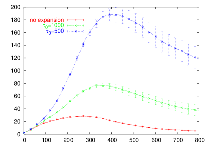
Figure 1: First mode of the structure function at different inverse expansion rates $\tau_{0}=500,1000,\infty$. Quench $\beta_{\xi}=5.5\rightarrow 5.92$ on $16^{3}$x$4$ lattice.

Note that in the standard application of anisotropic lattices (such as in Karsch:1982ve ) the space-like lattice spacing is not varied; the anisotropy is varied by decreasing the time-like lattice spacing. This procedure keeps the coupling within the scaling window provided the initial coupling is close to the continuum limit. Here, on the contrary, we keep the time-like spacing constant (or, later, slowly increase it) as we vary the space-like coupling. This induces changes in the coupling that may drive its value out of the scaling regime ($\beta\sim 5$). Therefore, our expansion has to be truncated whenever the value of $\beta$ falls below this cut-off value. This condition implies that, in order to follow the system evolution for longer time, one needs lattices with larger $N_{\tau}$, thus rendering the problem more computationally intensive.

We start simulations on smaller lattices where it is easier to gather satisfactory statistics for highly fluctuating quantities, such as the structure function. The quench is performed from $\beta_{\xi}=5.5$ to $\beta_{\xi}=5.92$ on $16^{3}$x$4$ lattice. The latter corresponds to a temperature after the quench $T_{\rm final}=1.57T_{c}$. The phase transition on this lattice at $\xi=1$ is at $\beta=5.6902(2)$. We use jack knife average over 10 bins, each of 50 configurations. The system is allowed to equilibrate for 200 lattice sweep, and then, after performing a quench, we allow the system to evolve for 800 sweeps, while measuring several lower modes of the structure function. We present here only averages of on-axis modes, such as permutations of $(n,0,0)$ - this is the n-th mode in our notation. The first modes are presented in Fig. 1. We see that expansion significantly enhances the response. The faster the expansion rate, the higher are the peaks. On the other hand the shift in the location of the peaks is not as pronounced, an important point to which we return below.

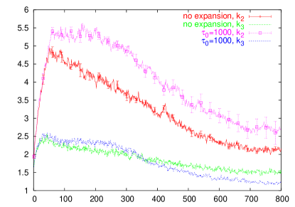
Figure 2: Higher ($k_{2}$ and $k_{3}$) structure function modes for non-expanding and $\tau_{0}=1000$ expanding system.

Next, we look at higher modes of the structure function in the cases of no expansion, and expansion at $\tau_{0}=1000$ – see Fig. 2. We see that the second mode shows behavior similar to that observed for the first mode. The difference, however, is not that significant. The third mode in the expanding system outgrows the corresponding mode in the non-expanding case at early times, but then decreases faster. This is an indication of the shift of the critical mode with time, observed in the linear effective model (section 2). At later times the transition proceeds only through the lower modes. The error bars for some of the data points are also presented in Fig. 1 and 2.

To make a comparison to the linear effective theory of Section 2, we make fits to the exponent for the structure function data (Fig. 3). We use a $32^{3}$x$4$ lattice since we know from previous studies Berg:2004qb ; Bazavov:2004wc that the linear response behavior (pertinent to early times) manifests itself better on the larger lattices. Contrary to our expectations from the linear theory of section 2, however, we find there no substantial change in the behavior of the exponent between the expanding and non-expanding systems. A fit to

$$S(\tau)\sim\exp(C\cdot\tau^{\alpha})$$

gives $\alpha=1.22$ for the expanding system, whereas it gives $\alpha=1.18$ for the non-expanding system. In Fig. 3 we also show fits to $S(\tau)\sim\exp(C\cdot\tau)$, which in fact provides the best fit per parameter degree of freedom. Both fits are over the $\tau$ range from $0$ to $250$. In any case, there is no substantial deviation from exponential growth with linear $\tau$ dependence in the exponent. Furthermore, from the figures we observe divergence from exponential behavior at later times $\tau>200$. Also notable is the enhancement of the signal (by a factor $\sim$ 7) in the expanding system as compared to the non-expanding system. All this provides a manifestation of the limitations of the linear response effective models in Section 2. We note that there are 10 times as many points for the fitting as on the plot.

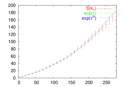
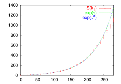
Figure 3: Fits to the exponent. Quenches on the $32^{3}$x$4$ lattice in non-expanding (top) and $\tau_{0}=500$ expanding (bottom) systems.

III.2 Expansion accompanied by temperature fall-off

In this second part of the numerical study we try to mimic conditions similar to those in heavy ion collisions at RHIC. We want to follow the evolution of the expanding and cooling QGP. We let the temperature drop as

$$T=\frac{T_{0}}{(1+\tau/\tau^{\prime}_{0})^{\alpha}}.$$ (23)

In the fire-tunnel (in the proper frame) the temperature is expected to decrease with the proper time $\tau$ as $T\sim\tau^{-1/3}$ or slower Bjorken:1983 . We adopt this value of $\alpha$ in the following.

We first work on smaller lattices for elucidating the main physical features. Therefore, we do not set the freeze-out condition (see below) and simply take $\tau^{\prime}_{0}=\tau_{0}$. With the $\alpha=1/3$ choice of temperature evolution, the anisotropy evolves as

$$\xi(\tau)=\left(1+\frac{\tau}{\tau_{0}}\right)^{2/3}$$ (24)

and $\beta$ evolves as in (22). We illustrate the effect of temperature drop on the structure function in Fig. 4.

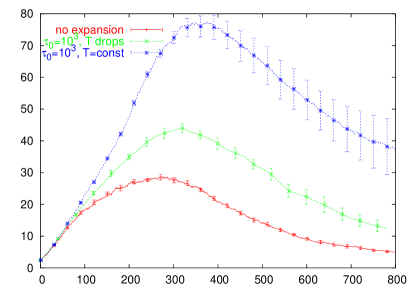
Figure 4: Comparison of first mode of structure functions including drop in temperature on a $16^{3}\times 4$ lattice (same quench as in Fig. 1).

There are two basic conclusions suggested by these plots.

The first is that the temperature evolution drives the system back towards the confined phase, but the expansion tends to prevent it as evidenced by the different peak heights. These are then two competing effects that tend to cancel, so that the return to structure function equilibration occurs at about the same time (here after about $700$ sweeps) as for the system in the absence of expansion and temperature fall-off. For the slower expansion rates ($\tau_{0}>1000$) and faster temperature fall-offs this cancellation effect is even more pronounced.

The second conclusion is suggested by the fact, also present and remarked upon in Fig. 1, that the location of the peaks is little affected by the presence of expansion and/or temperature evolution. This implies that the system’s response to the sudden quench is set by an internal dynamics scale that is faster than that of the expansion and accompanying temperature fall-off rates considered here. After the structure function is past its peak, the system is isotropized, and, after a relatively short time, any memory of the initial fast, spinodal-like, long range response to the violent quench across the deconfinemnt transition boundary disappears. The subsequent evolution is that of (quasi)equilibrium evolution of the system as it expands and cools towards its return to the confinement phase.

To elucidate this further we plot the time profile of the Polyakov loop average in Fig. 5 for the expanding and non-expanding systems as well as with and without drop in temperature. We now have to use a bigger, $32^{3}\times 8$ lattice in order to follow the evolution over a longer time interval.

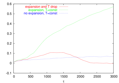
Figure 5: The Polyakov loop evolution after a quench in decreasing temperature on $32^{3}\times 8$ lattice (same initial and final temperature quench as in Fig. 1).

First note that pure expansion drives the Polyakov loop towards larger values, i.e. more pronounced deconfined behavior. To get some insight into this behavior observe that, as it is evident from (17), spatial expansion enhances the timelike part of the action (2nd term in the square brackets on the r.h.s.) while suppressing the spacelike parts F3 . This tends to increase the expectation of timelike Polyakov lines Fsan .

On the other hand, decreasing temperature counteracts the expansion effect. This is clearly seen in Fig. 5. Eventually, under the combined effects of expansion and temperature fall-off, the Polyakov loop expectations drops to zero signaling the return of the system to the confinement phase. These qualitative features of Fig. 5 are rather generic, being stable under changes in the expansion and temperature fall-off rates (cf. Fig. 6 below).

The crucial feature characterizing the system’s overall evolution following the rapid quench into the deconfinement region is clearly revealed by examining Fig. 5 in conjunction with the plots of the structure function in Fig. 4. It is the fact that there are two scales involved in this evolution. The first is the scale set by the location of the peak of the structure function; the second is the scale set by the interval to return to the confinement phase. Furthermore, there is wide separation between these two scales. As noted above, the location of the peak ($\sim 300$ in Fig. 4) is very little affected by the conditions of expansion and temperature fall-off. It reflects strongly coupled dynamics at short time scales driving the exponential growth of very long range modes F4 leading to ‘isotropization’, by which we mean nothing more specific than that the full development of these modes appear to completely wipe out any remnants of the quenching event. Rapid equilibration follows within an interval of a few hundreds sweeps ($\sim 300-400$ in fig. 4). The system then continues to evolve in quasi-equilibrium over a much longer period (typically of thousands of sweeps as in Fig. 5 and Fig. 6 below) expanding and cooling till it returns to the confinement phase. This separation of time scales is a very general feature over a wide range of parameters.

Having reached this qualitative physical picture, which accords well with that experimentally observed, it is interesting to explore whether it is possible to make an estimate of this separation in physical units, and establish some correspondence with heavy-ion collision phenomenology. This we do in the following subsection.

III.3 Isotropization-thermalization and chemical freeze-out times

The expansion and temperature variation parameters ($\tau_{0}^{\prime}$, $\tau_{0}$, $T_{\rm final}$) determine the precise time interval before returning to the confinement phase. Note that our requirement that the evolution remain inside the scaling window limits the time of observation. To deal with this and follow the evolution for substantial time we now work on a larger, $32^{3}$x$8$ lattice throughout, and attempt to set the parameters so as to reflect conditions in heavy ion collision at RHIC. There is strong evidence that the matter in the firetunnel reaches temperatures above $2T_{c}$ Kolb:2003dz . For our numerical simulation we quench to $T_{\rm final}\sim 3T_{c}$. (Note that $T_{c}$ here means critical temperature of pure gluodynamics). The system is equilibrated in the confinement phase at the same temperature as before $\approx 0.8T_{c}$. For $N_{\tau}=8$ and $\xi=1$ we recalculate the values of corresponding betas using the two-loop order formula connecting lattice spacing and the coupling, and reweigh it with non-perturbative correction factor above $T_{c}$ Boyd:1996bx . Such a correction is needed here since the bare gauge coupling is typically of order one for our range of betas. The value of $\beta_{c}$ is known from the lattice Polyakov loop susceptibility study Boyd:1996bx . We get

$$\beta_{\rm initial} =5.90 \quad 0.76T_{c}$$

$$\beta_{c} =6.0625 \quad T_{c}$$ (25)

$$\beta_{\rm final} =6.85 \quad 2.95T_{c}\;,$$

where ‘initial’ and ‘final’ refer to before and after the quench.

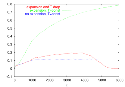
Figure 6: The Polyakov loop evolution after a quench to $2.95T_{c}$, $\tau_{0}=1000$

At high enough temperatures the system is close to an ideal gas of quasiparticles. Lattice data suggest that the equation of state does not actually deviate much from that of the ideal gas for all temperatures down to $T_{c}$, and is conveniently modeled as such in hydrodynamic descriptions. Hence, the energy and entropy densities scale as $e\sim T^{4}$ and $s\sim T^{3}$, respectively. Assuming adiabatic expansion the entropy per unit of rapidity is conserved. In real fire-tunnel evolution the initial expansion is one dimensional Bjorken:1983 , switching to three dimensional expansion at later times. This corresponds to $T\sim\tau^{-1/3}$ at the early and mid time and $T\sim\tau^{-1}$ at later time. The $T\sim\tau^{-1/3}$ behavior is in fact seen in the hydrodynamic evolution almost down to $T_{c}$ Heinz:2004pj ; Kolb:2003gq ; Kolb:2003dz , and is the only one considered in the following. We are thus led to modeling of the spatial expansion and temperature drop on the lattice in terms of the two parameters $\tau_{0}$ and $\tau_{o}^{\prime}$ as:

$$a_{s} = a_{0}(1+\frac{\tau}{\tau_{0}}),$$ (26)

$$a_{\tau} = a_{0}(1+\frac{\tau}{\tau_{0}^{\prime}})^{1/3}$$ (27)

$$= a_{0}(1+y\frac{\tau}{\tau_{0}})^{1/3},$$

where $y=\tau_{0}/\tau^{\prime}_{0}$ is the ratio of the ‘speeds’. The evolution of the anisotropy then is

$$\xi(\tau)=\frac{1+{\tau\over\tau_{0}}}{(1+y\,{\tau\over\tau_{0}})^{1/3}}$$ (28)

As the chemical freeze-out temperature we choose $T_{fo}=T_{c}$ Kolb:2003dz ; Heinz:2004pj ; Kolb:2003gq . Before this freeze-out the plasma undergoes an $x$-fold expansion

$$x=\frac{a_{s}}{a_{0}}=1+\frac{\tau_{fo}}{\tau_{0}}$$ (29)

On the other hand

$$\frac{T_{fo}}{T_{final}}=\frac{1}{(1+y\frac{\tau_{fo}}{\tau_{0}})^{1/3}}$$ (30)

From these two we get

$$y=\frac{(T_{final}/T_{fo})^{3}-1}{x-1}$$ (31)

Hydrodynamical model phenomenology yields all required parameters Kolb:2003gq . Thus we have $x\sim 9$ before the conversion to the confined phase is completed, and the freeze-out is observed. This corresponds to $y\sim 3.25$.

In Fig. 6 we plot the time profile of the Polyakov loop average in expanding and non-expanding systems with and without drop in temperature with these values of $x$, $y$, and $\tau_{0}=1000$. One again observes the same features discussed above in connection with Fig. 5.

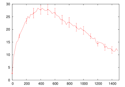
Figure 7: The first mode of structure function for non-expanding and constant $T$ system after a quench.

In Fig. 7 we show the lowest mode structure function in the case of no expansion and temperature variation. The expanding-variable temperature case is very similar. We see that at $\tau=400$ sweeps the system has reached the peak. This is the point of isotropisation of the system when the long range fluctuations reach through the system. It is again to be contrasted to the much longer times needed to return to confinement (vanishing Polyakov loop expectation).

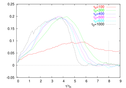
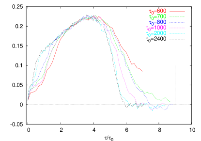
Figure 8: The Polyakov loop evolution after a quench to $2.95T_{c}$ for various values of $\tau_{0}$ and $x=9$ (top panel), $x=10$ (bottom panel).

To explore this difference in detail, in Fig. 8 we present the Polyakov loop average evolution at different expansion rates. The figure on the top panel uses again $x=9$, so the chemical freeze-out point on this plot is at $\tau/\tau_{0}=(x-1)=8$. We notice that in the range of $\tau_{0}\sim 400-600$ the Polyakov loop expectation value gets close to zero just before this point. Actually, this should be considered as a lower bound on the range of $\tau_{0}$’s since this is a first order transition (or a rapid crossover in the presence of fermions). Thus, there is a latent heat period during which the system lingers, with Polyakov loop expectations close to zero, before it is fully converted to the confined phase. The values $\tau_{0}=300$ and less (higher ‘speeds’) do not show this behavior and therefore do not lead to a consistent picture. Taking then the range of $\tau_{0}\gtrsim 400-600$ gives an interval to freeze-out of $\gtrsim 3200-4800$ sweeps, which in turn corresponds, from phenomenology, to $\sim 9fm/c$. This allows an upper bound estimate of the time around the peak of the structure function in physical units: $\lesssim 0.75-1.1\ fm/c$.

In the plot on the bottom panel in Fig. 8 we use the same quench to $2.95T_{c}$ but now take $x=10$, which gives $y=2.89$. This corresponds to a somewhat longer lifetime for the deconfined plasma. One sees that a value of $\tau_{0}\gtrsim 700-800$ gives a good fit to complete conversion to the confined phase by the time the freeze-out point is reached. This in turn gives $\lesssim 0.56-0.63\ fm/c$ as an upper bound estimate for the time around the peak of the structure function. There is of course an inherent uncertainty here as to what to take for the appropriate phenomenological value for the lifetime in physical units since we do not include fermions in out simulations; and fermions become important at the late stage of conversion back to confinement. In Fig. 8 we follow the curves as far as possible before running out of the scaling regime as explained in Section 3.1 above. Longer lifetimes result into even shorter isotropization times. To consider somewhat larger $x$ values, however, we need larger lattices than those employed in this study. But the main message extracted from the present decimations should be clear. The robust separation between the ‘fast’ dynamics scale of the exponential growth of the spinodal-like response to the sudden quench and that set by return to confinement is such that isotropization times well inside $1\ fm/c$ result naturally for any reasonable choice of parameters.

IV Conclusions

In this paper we studied the response of the pure $SU(3)$ gauge theory to a rapid quench from its confined to its deconfined phase. In a series of simulations we followed the subsequent evolution of the system under varying conditions of temperature fall-off and/or spatial expansion. These conditions were chosen so as to reflect the type of variations presumed to hold in heavy ion collisions. Our main finding is that there are two distinct scales characterizing this evolution. There is one scale set by the development of very long range modes continuously from zero to their maximum amplitude over a short time interval. These modes, manifested in the response of the structure functions to the quench, drive isotropization and return to thermalization shortly afterwards. The scale set by this ‘fast’ dynamics is little affected by conditions of expansion and temperature variations. The second scale is set by the time interval to return to the confinement phase under quasi-equilibrium evolution, and is affected by the details of expansion and temperature fall-off. There is a robust wide separation between the two scales, which, translated to physical units under reasonable assumptions about the lifetime of the plasma, gives estimates of the ‘fast’ dynamics in the range of $0.5-1\ fm/c$.

There is a number of directions in which this study can be extended. The formalism used above can be extended to treat also anisotropy among the different space directions, thus allowing a more ‘realistic’ treatment of spatial expansion. Whether this makes much of difference, however, remains to be seen (cf. footnote Fsan ). Another interesting question is that concerning the effect of having a really finite physical system. In our simulations we, as usual, employed periodic boundary conditions. But one may explore different ones that would mimic a finite rather than an infinite system. The other obvious extension is the inclusion of fermions. The deconfinement transition is driven by gluonic dynamics. Fermions, however, are expected to contribute more substantially at the late stage of return to confinement and hadronization. Thus our study applies strictly to the gluonic plasma. Nonetheless, the qualitative picture of the separation of scales found above should not be affected in an essential way by the inclusions of fermions, though quantitative details related to the exact lifetime of the plasma, etc certainly will.

References

- (1) U. W. Heinz, AIP Conf. Proc. 739, 163 (2005) [arXiv:nucl-th/0407067].
- (2) P. F. Kolb, Heavy Ion Phys. 21, 243 (2004) [arXiv:nucl-th/0304036].
- (3) P. F. Kolb and U. W. Heinz, arXiv:nucl-th/0305084.
- (4) D. Molnar and M. Gyulassy, Nucl. Phys. A 697, 495 (2002).
- (5) J. Bjoraker and R. Venugopalan, Phys. Rev. C 63, 024609 (2001).
- (6) R. Baier, A.H. Mueller, D. Schiff, D.T. Son, Phys. Lett. B 539, 46 (2002); ibid. 502, 51 (2001).
- (7) D. Kharzeev, arXiv:hep-ph/0408091.
- (8) E. Iancu and R. Venugopalan, arXiv:hep-ph/0303204.
- (9) Y.V. Kovchegov, arXiv:hep-ph/0503038; arXiv:hep-ph/0507134.
- (10) P. Arnold, J. Lenaghan and G.D. Moore, JHEP 0308, 002 (2003); P. Arnold and J. Lenaghan, Phys. Rev. D 70, 114007 (2004).
- (11) P. Romatschke and M. Strickland, Phys. Rev. D 68, 036004 (2003) [arXiv:hep-ph/0304092].
- (12) S. Mrowczynski, Phys. Lett. B 393, 26 (1997); 314, 118 (1993); Phys. Rev. C 49, 2191 (1994).
- (13) U.W. Heinz, Nucl. Phys. A 418, 603C (1984).
- (14) P. Arnold, J. Lenaghan, G.D. Moore and L.G. Yaffe, Phys. Rev. Lett. 94, 072302 (2005).
- (15) A. Rebhan, P. Romatschke and M. Strickland, Phys. Rev. Lett. 94, 102303 (2005) [arXiv:hep-ph/0412016].
- (16) P. Romatschke and M. Strickland, Phys. Rev. D 70, 116006 (2004) [arXiv:hep-ph/0406188]; S. Mrowczynski, A. Rebhan and M. Strickland, Phys. Rev. D 70, 025004 (2004) [arXiv:hep-ph/0403256].
- (17) A. Dumitru and Y. Nara, arXiv:hep-ph/0503121.
- (18) C. Manuel and S. Mrowczynski, arXiv:hep-ph/0504156.
- (19) P. Arnold, G.D. Moore and L.G. Yaffe, arXiv:hep-ph/0505212.
- (20) A. Rebhan, P. Romatschke and M. Strickland, arXiv:hep-ph/0505261.
- (21) J. D. Gunton and M. Droz, ”Introduction to the Theory of Metastable and Unstable States”, Springer-Verlag (1985).
- (22) P. M. Chaikin and T. C. Lubensky”, ”Principles of condensed matter physics”, Cambridge University Press (1997).
- (23) R. D. Pisarski, Phys. Rev. D 62, 111501 (2000) [arXiv:hep-ph/0006205].
- (24) N. Weiss, Phys. Rev. D 24, 475 (1981); ibid, 25, 2667 (1982).
- (25) T. Heinzl, T. Kaestner and A. Wipf, arXiv:hep-lat/0502013.
- (26) J. D. Gunton, M. San Miguel and P. S. Sahni, in “Phase Transitions and Critical Phenomena, v. 8”, C. Domb and J. L. Lebowitz (editors), Academic Press (1983).
- (27) T. R. Miller and M. C. Ogilvie, Phys. Lett. B 488, 313 (2000) [arXiv:hep-lat/0004004].
- (28) T. R. Miller and M. C. Ogilvie, Nucl. Phys. Proc. Suppl. 94, 419 (2001) [arXiv:hep-lat/0010055].
- (29) T. R. Miller and M. C. Ogilvie, Nucl. Phys. Proc. Suppl. 106, 537 (2002) [arXiv:hep-lat/0110109].
- (30) A. Bazavov, B. A. Berg and A. Velytsky, arXiv:hep-lat/0410019.
- (31) B. A. Berg, U. M. Heller, H. Meyer-Ortmanns and A. Velytsky, Nucl. Phys. Proc. Suppl. 129, 587 (2004) [arXiv:hep-lat/0308032].
- (32) B. A. Berg, U. M. Heller, H. Meyer-Ortmanns and A. Velytsky, Phys. Rev. D 69, 034501 (2004) [arXiv:hep-lat/0309130].
- (33) B. A. Berg, H. Meyer-Ortmanns and A. Velytsky, Phys. Rev. D 70, 054505 (2004) [arXiv:hep-lat/0405011].
- (34) A. Velytsky, B. A. Berg and U. M. Heller, Nucl. Phys. Proc. Suppl. 119, 861 (2003) [arXiv:hep-lat/0208035].
- (35) J. W. Cahn and J. E. Hilliard, J. Chem. Phys. 28, 258 (1958).
- (36) A. Velytsky, Ph.D. thesis, UMI-31-37501
- (37) An alternative dynamical model based on an extension of (1) that includes a chiral field, and involving second-order time derivatives was introduced in Scavenius:2001pa . It was used to study the transition back into the confinement phase at the end of the QGP evolution, in contrast to our first-order model used here to study the initial response right after the quench into the deconfinement phase.
- (38) O. Scavenius, A. Dumitru and A. D. Jackson, Phys. Rev. Lett. 87, 182302 (2001) [arXiv:hep-ph/0103219].
- (39) J. D. Bjorken, Phys. Rev. D 27, 140 (1983).
- (40) F. Karsch, Nucl. Phys. B 205, 285 (1982).
- (41) The effect is qualitatively similar to that of having no spatial expansion but, instead, raising the temperature.
- (42) We parenthetically remark that this observation leads to the expectation that, as far as the behavior of the timelike Polyakov line is concerned, the difference between 3-dimensional and 1-dimensional spatial expansion may be numerically not all that significant. (Clearly, this may be not be the case for other physical quantities.) This is because, as seen from (17), such a difference affects only the degree of expansion-induced suppression of interactions in the different space directions, but not the expansion-induced enhancement of the timelike interactions; and it is the latter that mainly affects the Polyakov loop enhancement under expansion seen in Fig. 5. Whether this expectation concerning changes in the dimensionality of the spatial expansion is indeed correct remains, of course, to be decided by actual computations not carried out in this paper.
- (43) It is worth noting again that all higher momentum modes are essentially unaffected in this type of response to the quench, a somewhat counter-intuitive behavior, which, however, is well known in spinodal-like responses.
- (44) G. Boyd, J. Engels, F. Karsch, E. Laermann, C. Legeland, M. Lutgemeier and B. Petersson, Nucl. Phys. B 469, 419 (1996) [arXiv:hep-lat/9602007].
- (45) R. G. Edwards and B. Joo [SciDAC Collaboration], arXiv:hep-lat/0409003.