Abstract

We examine the effects of the extended gauge sector of the Littlest Higgs model in high energy $e^{+}e^{-}$ collisions. We find that the search reach in $e^{+}e^{-}\rightarrow f\bar{f}$ at a $\sqrt{s}=500\,{\mathrm{GeV}}$ International Linear Collider covers essentially the entire parameter region where the Littlest Higgs model is relevant to the gauge hierarchy problem. In addition, we show that this channel provides an accurate determination of the fundamental model parameters, to the precision of a few percent, provided that the LHC measures the mass of the heavy neutral gauge field. Additionally, we show that the couplings of the extra gauge bosons to the light Higgs can be observed from the process $e^{+}e^{-}\rightarrow Zh$ for a significant region of the parameter space. This allows for confirmation of the structure of the cancelation of the Higgs mass quadratic divergence and would verify the little Higgs mechanism.

1 Introduction

The Standard Model (SM) of particle physics is a remarkably successful theory. It provides a complete description of physics at currently accessible energies, and its predictions have been confirmed to high accuracy by all high energy experiments to date. An important piece of the SM remains unexplained–the mechanism of electroweak symmetry breaking. Precision measurements and direct searches suggest that this mechanism involves a weakly coupled Higgs boson with a mass in the range $114<m_{H}<208\,{\mathrm{GeV}}$ at 95% CL. The Higgs mass parameter, however, is quadratically sensitive to UV physics. New physics at the  TeV scale is therefore necessary to keep the Higgs light without fine-tuning. This is known as the hierarchy problem. Three main classes of models, supersymmetry, extra dimensions, and little Higgs, have been proposed to address the hierarchy problem. Which of these theories Nature has chosen will be determined in the coming years as the Large Hadron Collider and the International Linear Collider probe the  TeV scale.

The little Higgs models [1, 2, 3] feature the Higgs as a pseudo Nambu-Goldstone boson of an approximate global symmetry which is broken by a vev at a scale of a few  TeV. The breaking is realized in such a way that the Higgs mass only receives quantum corrections at two loops. In contrast to supersymmetry, the one-loop contribution to the Higgs mass from a SM particle is canceled by a contribution from a new particle of the same spin. Little Higgs theories thus predict the existence of new top-like quarks, gauge bosons, and scalars near the  TeV scale. The distinguishing features of this model are the existence of these new particles and their couplings to the light Higgs. Measurement of these couplings would verify the structure of the cancelation of the Higgs mass quadratic divergences and prove the existence of the little Higgs mechanism.

The most economical little Higgs model is the so-called “Littlest Higgs” (LH) [1], which we introduce here and describe in more detail in Sec. 2. This scenario is based on a non-linear sigma model with an $SU(5)$ global symmetry, which is broken to the subgroup $SO(5)$ by a vev $f$. The vev is generated by some strongly coupled physics at a scale $\Lambda_{S}\sim 4\pi f$; possible UV completions of little Higgs theories are discussed in [3, 4]. The $SU(5)$ contains a gauged subgroup $[SU(2)\times U(1)]^{2}$ which is broken by the vev to the SM electroweak group $[SU(2)_{L}\times U(1)_{Y}]$. The global $SU(5)$ breaking leaves 14 massless Goldstone bosons, four of which are eaten by the gauge bosons of the broken gauge groups, giving these gauge bosons a mass of order $f$. In particular, we have a heavy $Z$-like boson $Z_{H}$ and a heavy photon-like boson $A_{H}$ which, as we will see, are phenomenologically important. The other ten Goldstone bosons make up a complex doublet and a complex triplet which remain massless at this stage. Masses for the complex triplet are generated at the  TeV-scale by one-loop gauge interactions. The neutral component of the complex doublet plays the role of the SM Higgs. Its mass term comes from a Coleman-Weinberg potential and has quadratically divergent corrections only at two loops, giving $\mu^{2}\sim f^{2}/16\pi^{2}$. Thus the natural scale for $f$ is around a  TeV. If $f$ is much higher than a few  TeV, the Higgs mass must again be finely tuned and this model no longer addresses the hierarchy problem.

The phenomenological implications of little Higgs models have been explored in [1, 5, 6, 7, 8, 9, 10, 11]. Constraints arise from electroweak precision data as well as from indirect and direct production at LEP-II and the Tevatron. For example, in the Littlest Higgs scenario, the lack of discovery of the $A_{H}$, which is expected to be quite light, puts a lower bound on $f$ in the few  TeV range. Significant electroweak constraints come from tree-level and loop deviations of the $\rho$-parameter and the weak mixing angle $\sin^{2}\theta_{w}$ from their SM values. Combining these gives a limit $f\mathrel{\mathchoice{\lower 3.01385pt\vbox{\halign{$\matth\displaystyle\hfil#\hfil$\cr>\crcr\sim\crcr}}}{\lower 3.01385pt\vbox{\halign{$\matth\textstyle\hfil#\hfil$\cr>\crcr\sim\crcr}}}{\lower 3.01385pt\vbox{\halign{$\matth\scriptstyle\hfil#\hfil$\cr>\crcr\sim\crcr}}}{\lower 3.01385pt\vbox{\halign{$\matth\scriptscriptstyle\hfil#\hfil$\cr>\crcr\sim\crcr}}}}4\,{\mathrm{TeV}}$ which is relatively parameter independent. Many variants of little Higgs models exist in the literature which lower this bound to $f\mathrel{\mathchoice{\lower 3.01385pt\vbox{\halign{$\matth\displaystyle\hfil#\hfil$\cr>\crcr\sim\crcr}}}{\lower 3.01385pt\vbox{\halign{$\matth\textstyle\hfil#\hfil$\cr>\crcr\sim\crcr}}}{\lower 3.01385pt\vbox{\halign{$\matth\scriptstyle\hfil#\hfil$\cr>\crcr\sim\crcr}}}{\lower 3.01385pt\vbox{\halign{$\matth\scriptscriptstyle\hfil#\hfil$\cr>\crcr\sim\crcr}}}}1-2\,{\mathrm{TeV}}$.

In this paper we use the processes $e^{+}e^{-}\rightarrow f\bar{f}$ and $e^{+}e^{-}\rightarrow Zh$ to investigate experimental limits from LEP II data on the Littlest Higgs parameters, to evaluate the extent of the International Linear Collider’s search reach in LH parameter space, and to see how accurately the ILC will be able to determine the LH parameters. We will see that the ILC can substantially extend the discovery reach of the LHC. In addition, we will also see that the bounds from $e^{+}e^{-}\rightarrow f\bar{f}$ at LEP II exclude a large part of the LHC’s search reach in the $pp\rightarrow Z_{H}\rightarrow Z_{L}h\rightarrow\ell^{+}\ell^{-}b\bar{b}$ channel. Complementary discussions of the Littlest Higgs model at the ILC and LHC can be found in [10, 11]. In Sec. 2, we discuss the Littlest Higgs model in detail. In Sec. 3, we examine the process $e^{+}e^{-}\rightarrow f\bar{f}$ at LEP II and the ILC and determine how accurately the ILC will be able to measure the LH parameters. In Sec. 4 we explore the LH parameter space using the process $e^{+}e^{-}\rightarrow Zh$ at the ILC.

2 The Littlest Higgs model and its parameters

In this paper, we are mainly concerned with the extended neutral gauge sector present in the LH model. While this scenario also includes a number of parameters that arise from the top and scalar sectors, in which there are a number of new heavy particles, the observables of concern in our analysis only depend on the three parameters present in the extended heavy gauge sector. These are $f$, the vev or “pion decay constant” of the nonlinear sigma model, which we discussed in the Introduction, and two mixing angles. Although we focus on the Littlest Higgs model, we note that an enlarged gauge sector with rather generic features is present in all little Higgs scenarios.

The vev $f$ characterizes the scale of the $SU(5)\rightarrow SO(5)$ breaking; the effective field theory of the 14 Goldstone bosons has the Lagrangian

$${\cal L}_{\Sigma}=\frac{1}{2}\frac{f^{2}}{4}\mbox{Tr}\left|{\cal D}_{\mu}\Sigma\right|^{2},$$ (1)

where $\Sigma$ is a $5\times 5$ matrix parametrization of the Goldstone boson degrees of freedom [1, 11]. The covariant derivative contains the gauge bosons associated with the gauged subgroup $[SU(2)\times U(1)]^{2}$, $W_{1}$, $W_{2}$, $B_{1}$, and $B_{2}$;

$${\cal D}_{\mu}\Sigma=\partial_{\mu}\Sigma-i\sum^{2}_{j=1}\left(g_{j}(W_{j}\Sigma+\Sigma W_{j}^{T})+g^{\prime}_{j}(B_{j}\Sigma+\Sigma B^{T}_{j})\right).$$ (2)

At the same time, the $[SU(2)\times U(1)]^{2}$ is also broken to $[SU(2)_{L}\times U(1)_{Y}]$, and the gauge boson mass eigenstates after the symmetry breaking are

$$\begin{split}W=sW_{1}+cW_{2},\;\;\;&W^{\prime}=-cW_{1}+sW_{2},\\ B=s^{\prime}B_{1}+c^{\prime}B_{2},\;\;\;&B^{\prime}=-c^{\prime}B_{1}+s^{\prime}B_{2}.\end{split}$$ (3)

The $W$ are the massless gauge bosons associated with the generators of $SU(2)_{L}$ and the $B$ is the massless gauge boson associated with the generator of $U(1)_{Y}$. The $W^{\prime}$ and $B^{\prime}$ are the massive gauge bosons associated with the four broken generators of $[SU(2)\times U(1)]^{2}$, with their masses being given by

$$m_{W^{\prime}}=\frac{f}{2}\sqrt{g_{1}^{2}+g_{2}^{2}}=\frac{g}{2sc}f,\;\;\;m_{B^{\prime}}=\frac{f}{2\sqrt{5}}\sqrt{{g_{1}^{\prime}}^{2}+{g_{2}^{\prime}}^{2}}=\frac{g}{2\sqrt{5}s^{\prime}c^{\prime}}f.$$ (4)

The mixing angles

$$s=\frac{g_{2}}{\sqrt{g_{1}^{2}+g_{2}^{2}}}\;\;\mbox{and}\;\;s^{\prime}=\frac{g_{2}^{\prime}}{\sqrt{g_{1}^{\prime 2}+g_{2}^{\prime 2}}}$$ (5)

relate the coupling strengths of the two copies of $[SU(2)\times U(1)]$. These two angles together with $f$ are the three parameters of the model that are relevant to our analysis. As we will see, the factor of $\sqrt{5}$ in the denominator of the expression for $m_{B^{\prime}}$ will have important phenomenological consequences.

The Higgs sector contains a scalar triplet in addition to a SM-like scalar doublet. The doublet and triplet both obtain vevs. The doublet vev, $v$, brings about electroweak symmetry breaking (EWSB) as in the SM, and thus $v=246\,{\mathrm{GeV}}$. The triplet vev, $v^{\prime}$, is related to $v$ by the couplings in the Coleman-Weinberg potential. Taking these to be $\mathcal{O}(1)$ gives the relation $v^{\prime}\simeq v^{2}/2f$.

After EWSB, the mass eigenstates are obtained via mixing between the heavy ($W^{\prime}$ and $B^{\prime}$) and light ($W$ and $B$) gauge bosons. They include the light (SM-like) bosons $W^{\pm}_{L}$, $Z_{L}$, and $A_{L}$ observed in experiment, and new heavy bosons $W^{\pm}_{H}$, $Z_{H}$, and $A_{H}$ that could be observed in future experiments. At tree level, the processes $e^{+}e^{-}\rightarrow f\bar{f}$ and $e^{+}e^{-}\rightarrow Zh$ involve the exchange of only the neutral gauge bosons. Their masses are given to $\mathcal{O}(v^{2}/f^{2})$ by

$$\begin{split}M^{2}_{A_{L}}&=0,\\ M^{2}_{Z_{L}}&=m^{2}_{Z}\left[1-\frac{v^{2}}{f^{2}}\left(\frac{1}{6}+\frac{1}{4}(c^{2}-s^{2})^{2}+\frac{5}{4}(c^{\prime 2}-s^{\prime 2})^{2}\right)+8\frac{v^{\prime 2}}{v^{2}}\right],\\ M^{2}_{A_{H}}&=m^{2}_{Z}s^{2}_{w}\left[\frac{f^{2}}{5s^{\prime 2}c^{\prime 2}v^{2}}-1+\frac{v^{2}}{2f^{2}}\left(\frac{5(c^{\prime 2}-s^{\prime 2})^{2}}{2s_{w}^{2}}-x_{H}\frac{g}{g^{\prime}}\frac{c^{\prime 2}s^{2}+c^{2}s^{\prime 2}}{cc^{\prime}ss^{\prime}}\right)\right],\\ M^{2}_{Z_{H}}&=m^{2}_{W}\left[\frac{f^{2}}{s^{2}c^{2}v^{2}}-1+\frac{v^{2}}{2f^{2}}\left(\frac{(c^{2}-s^{2})^{2}}{2c_{w}^{2}}+x_{H}\frac{g^{\prime}}{g}\frac{c^{\prime 2}s^{2}+c^{2}s^{\prime 2}}{cc^{\prime}ss^{\prime}}\right)\right],\\ \end{split}$$ (6)

where $m_{W}$ and $m_{Z}$ are the SM gauge boson masses, and $s_{w}$ ($c_{w}$) represents the sine (cosine) of the weak mixing angle. Here $x_{H}$, given by [11]

$$x_{H}=\frac{5}{2}gg^{\prime}\frac{scs^{\prime}c^{\prime}(c^{2}{s^{\prime}}^{2}+s^{2}{c^{\prime}}^{2})}{5g^{2}{s^{\prime}}^{2}{c^{\prime}}^{2}-{g^{\prime}}^{2}s^{2}c^{2}},$$ (7)

characterizes the mixing between $B^{\prime}$ and $W^{\prime 3}$ in the $A_{H}$ and $Z_{H}$ eigenstates. It is important to note that all but the first term in the square brackets for $M^{2}_{A_{H}}$ and $M^{2}_{Z_{H}}$ are numerically insignificant. Thus $M^{2}_{A_{H}}$ depends strongly on $s^{\prime}$ and not on $s$, and vice versa for $M^{2}_{Z_{H}}$. This dependence is shown in Fig. 1. Note that the $A_{H}$ is significantly lighter than the $Z_{H}$ and can be as light as a few hundred  GeV; we will discuss the consequences of this below.

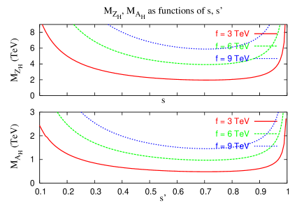
Figure 1: (Color online) Dependence of the heavy gauge boson masses $M_{Z_{H}}$ and $M_{A_{H}}$ on $s$ and $s^{\prime}$, respectively, for different values of $f$.

After EWSB, the couplings of the gauge bosons $Z_{L}$, $A_{H}$, and $Z_{H}$ to fermions similarly depend on $s$, $s^{\prime}$ and $f$ because of the mixing between the fields. If we demand that the U(1) be anomaly-free, which requires $y_{u}=-2/5$ and $y_{e}=3/5$ in the notation of [11], the general structure of the couplings is

$$\begin{split}g(A_{L}f\bar{f})&=g_{SM}(Af\bar{f}),\\ g(Z_{L}f\bar{f})&=g_{SM}(Zf\bar{f})\left(1+\frac{v^{2}}{f^{2}}a_{i}(s,s^{\prime})\right),\\ g(A_{H}f\bar{f})&=b_{i}\frac{g^{\prime}}{2s^{\prime}c^{\prime}}(\frac{1}{5}-\frac{1}{2}{c^{\prime}}^{2}),\\ g(Z_{H}f\bar{f})&=\pm\frac{gc}{4s},\end{split}$$ (8)

where $g_{SM}$ represents the relevant coupling in the SM. A and Z are the SM photon and Z boson, and $a_{i}$ and $b_{i}$ are both $\mathcal{O}(1)$ where $i$ labels the species of fermion.

The existence of the heavy gauge boson-Higgs couplings is a hallmark of the Littlest Higgs model. They can be probed using the process $e^{+}e^{-}\rightarrow Z_{L}H$ through the exchange of the $Z_{L}$, $Z_{H}$, and $A_{H}$. The relevant couplings are given by

$$\begin{split}g(Z_{L\mu}Z_{L\nu}H)&=g_{SM}(Z_{\mu}Z_{\nu}H)\left(1+\frac{v^{2}}{f^{2}}a(s,s^{\prime})\right),\\ g(Z_{L\mu}Z_{H\nu}H)&=\frac{-i}{2}\frac{g^{2}}{c_{W}}v\frac{c^{2}-s^{2}}{2sc}g_{\mu\nu},\\ g(Z_{L\mu}A_{H\nu}H)&=\frac{-i}{2}\frac{gg^{\prime}}{c_{W}}v\frac{c^{\prime 2}-s^{\prime 2}}{2s^{\prime}c^{\prime}}g_{\mu\nu}.\end{split}$$ (9)

where $a$ is an $\mathcal{O}(1)$ function. The formulae for the couplings can be found in Appendix B of the first paper in [11].

Certain bounds on $s$ and $s^{\prime}$ can be obtained by requiring that these couplings remain perturbative. Using the convention that a perturbative coupling $g$ satisfies $g^{2}/4\pi<1$ gives $s,s^{\prime}\mathrel{\mathchoice{\lower 3.01385pt\vbox{\halign{$\matth\displaystyle\hfil#\hfil$\cr>\crcr\sim\crcr}}}{\lower 3.01385pt\vbox{\halign{$\matth\textstyle\hfil#\hfil$\cr>\crcr\sim\crcr}}}{\lower 3.01385pt\vbox{\halign{$\matth\scriptstyle\hfil#\hfil$\cr>\crcr\sim\crcr}}}{\lower 3.01385pt\vbox{\halign{$\matth\scriptscriptstyle\hfil#\hfil$\cr>\crcr\sim\crcr}}}}0.1-0.2$. Using the more conservative convention $g^{2}<1$ would give a smaller allowed range for the parameters. In the analysis that follows, we include the region where $s>0.16$. As discussed above, expectations for the value of $f$ arise from the requirement of naturalness. For $f\mathrel{\mathchoice{\lower 3.01385pt\vbox{\halign{$\matth\displaystyle\hfil#\hfil$\cr>\crcr\sim\crcr}}}{\lower 3.01385pt\vbox{\halign{$\matth\textstyle\hfil#\hfil$\cr>\crcr\sim\crcr}}}{\lower 3.01385pt\vbox{\halign{$\matth\scriptstyle\hfil#\hfil$\cr>\crcr\sim\crcr}}}{\lower 3.01385pt\vbox{\halign{$\matth\scriptscriptstyle\hfil#\hfil$\cr>\crcr\sim\crcr}}}}10\,{\mathrm{TeV}}$, the LH model no longer addresses the hierarchy problem.

As in [11], we write the fermion-boson coupling as $i\gamma^{\mu}(g_{V}+g_{A}\gamma^{5})$. It turns out that for the electron-$Z_{L}$ coupling, $|g_{A}|\gg|g_{V}|$, while in general the shifts in the couplings due to mixing are roughly equal, i.e $|\Delta g_{A}|\simeq|\Delta g_{V}|$. Thus the relative change in $g_{V}$ is in general much greater than that for $g_{A}$, as shown in Fig. 2.

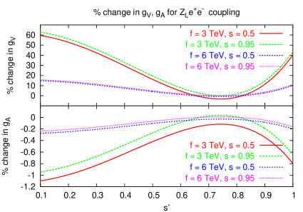
Figure 2: (Color online) The percent deviation of the vector and axial $Z_{L}e\bar{e}$ couplings from the SM values for $Z_{SM}e\bar{e}$, taking various values for the parameters f and s.

This relative change in $g_{V}$ is numerically fairly unimportant for most of the observables in our analysis, as the cross sections are typically functions of $g_{V}^{2}+g_{A}^{2}$. The left-right asymmetry $A_{LR}$, however, has terms directly proportional to $g_{V}$. Therefore, for the ILC, which has beam polarization capability, the $A_{LR}$ deviation is important and introduces a surprising $s^{\prime}$ dependence in our results. We will discuss this in greater detail in Sec. 3.

Equation 6 shows that for generic choices of $s$ and $s^{\prime}$, $M_{A_{H}}/M_{Z_{H}}\simeq s_{w}m_{Z}/\sqrt{5}m_{W}\simeq 1/4$. Figure 1 illustrates this, with $M_{A_{H}}$ dipping well below 1  TeV  for much of the parameter space. As mentioned in Sec. 1, this light $A_{H}$ is responsible for the most stringent experimental constraints on the model [5, 9]. As a result, phenomenologically viable variations of the Littlest Higgs models typically decouple the $A_{H}$ by modifying the gauge structure of the theory as in [12] and [13]. In this paper, however, we analyze the original Littlest Higgs model as it is the most phenomenologically well-studied. To gain some understanding of models in which the $A_{H}$ decouples we take two approaches in our analysis. One is to choose a parameter value ($s^{\prime}=\sqrt{3/5}$) for which the coupling of $A_{H}$ to fermions vanishes. This decouples the $A_{H}$ from all tree-level electron-positron collider physics. Another approach is to artificially take $M_{A_{H}}\rightarrow\infty$ while letting all other quantities in the theory take on their usual, parameter-dependent values. While not theoretically consistent, this approach gives us a more general picture of the behavior of models in which the $A_{H}$ decouples. We take both approaches and show the results for each case throughout our analysis.

3 Parameter Determination via $e^{+}e^{-}$$\rightarrow$ $f\bar{f}$

In this section we examine the process $e^{+}e^{-}\rightarrow f\bar{f}$, where all of the LH neutral gauge bosons participate via s-channel exchange, at past and future colliders. We first use a $\chi$-square analysis using the $e^{+}e^{-}\rightarrow f\bar{f}$ observables measured at LEP II. This analysis gives the region of LH parameter space excluded (to 95% confidence level) by the LEP II data.

We then perform a similar $\chi$-square analysis at the energies and luminosity expected at the ILC. We use the same set of observables as in the LEP II analysis as well as the polarization asymmetries that will be measurable due to the beam polarization capability at the ILC. This analysis gives the region of LH parameter space for which the ILC will be able to determine (to 95% confidence level) that the data cannot be explained by the Standard Model, and represents the ILC Littlest Higgs search reach. The two analyses just mentioned are described in Sec. 3.1.

Finally, in Sec. 3.2, we examine the ability of the ILC to determine the values of the LH parameters from $e^{+}e^{-}\rightarrow f\bar{f}$. For a few different generic sets of LH parameters, we first generate sample data for the observables, and then perform a $\chi$-square analysis to map out the region in LH parameter space that is inconsistent (to 95% CL) with the sample data. The size and shape of the remaining region tells us how accurately LH parameters can be determined.

3.1 The LEP II exclusion region and ILC search reach

Here we present our numerical analysis of the experimental constraints on the Littlest Higgs parameter space from LEP II data as well as the search reach expected from the ILC. We use the Lagrangian and Feynman rules of the Littlest Higgs model as described in [11]. Note that for our analysis, we follow the notation of [11] and take the values of the U(1) charge parameters $y_{u}=-2/5$ and $y_{e}=3/5$ that, as previously discussed, leave the U(1) anomaly-free and give the couplings shown in Eq. 8. The remaining free parameters of the model that are relevant to $e^{+}e^{-}\rightarrow f\bar{f}$ are the sines of the two $[SU(2)\times U(1)]$ mixing angles, $s$ and $s^{\prime}$; and the “decay constant,” or vev, $f$ as defined in Eq. 1 and Eq. 5.

We first study the constraints on the model from $e^{+}e^{-}\rightarrow f\bar{f}$ at LEP II, taking as our observables the normalized, binned angular distribution and total cross section for $e^{+}e^{-}\rightarrow$$b\bar{b}$, $c\bar{c}$, and $l\bar{l}$, with $l=e$, $\mu$, or $\tau$. We use $\sqrt{s}=200\,{\mathrm{GeV}}$ and an integrated luminosity ${\cal L}$= 627  ${\mathrm{pb}}^{-1}$. For the detection efficiencies, we take $\epsilon_{e}$ = 97%, $\epsilon_{\mu}$ = 88%, $\epsilon_{\tau}$ = 49%, $\epsilon_{b}$ = 40%, and $\epsilon_{c}$ = 10%  [14]. We perform a $\chi$-square analysis and take the SM values for all the observables to correspond to $\chi^{2}=0$, with a nonzero $\chi^{2}$ representing deviation from the SM. This is a reasonable approach, since there was no detectable deviation from the SM at LEP II [14].

For the ILC analysis, in addition to the above mentioned observables, we also include the angular binned left-right asymmetry $A_{LR}$ for each fermion pair. We use the projected energy $\sqrt{s}=500\,\,{\mathrm{GeV}}$ and luminosity ${\cal L}$= 500  ${\mathrm{fb}}^{-1}$. For the detection efficiencies, we take $\epsilon_{e}$ = 97%, $\epsilon_{\mu,\tau}$ = 95%, $\epsilon_{b}$ = 60%, and $\epsilon_{c}$ = 35% [15].

Because of the presence of the $Z_{H}$ and $A_{H}$, we use a general formula for the differential cross section for $e^{+}e^{-}\rightarrow f\bar{f}$ that is valid for any set of extra gauge bosons that can run in the s-channel [16],

$$\frac{d\sigma}{dz}=C_{\rm f}\frac{s}{32\pi}\sum_{ij}P_{ij}^{ss}[B_{ij}(1+z^{2})+2C_{ij}z],$$ (10)

where $z\equiv\cos\theta$, $C_{\rm f}$ is the color factor,

$$P_{ij}^{ss}\equiv\frac{(s-M_{i}^{2})(s-M_{j}^{2})+(\Gamma_{i}M_{i})(\Gamma_{j}M_{j})}{[(s-M_{i}^{2})^{2}+(\Gamma_{i}M_{i})^{2}][(s-M_{j}^{2})^{2}+(\Gamma_{j}M_{j})^{2}]},$$ (11)

and

$$B_{ij}\equiv(v_{i}v_{j}+a_{i}a_{j})_{f}(v_{i}v_{j}+a_{i}a_{j})_{e}\,,\;C_{ij}\equiv(v_{i}a_{j}+a_{i}v_{j})_{f}(v_{i}a_{j}+a_{i}v_{j})_{e}.$$

Here $v$ and $a$ correspond to the vector and axial couplings $g_{V}$ and $g_{A}$ discussed in Sec. 2, and the sum runs over the gauge bosons in the s-channel: $A_{L}$, $Z_{L}$, $A_{H}$, and $Z_{H}$.

For Bhabha scattering, besides the s-channel, we also have a contribution from the t-channel, so that

$$\begin{split}\frac{d\sigma}{dz}=\frac{s}{32\pi}\sum_{ij}\bigg{\{}&P_{ij}^{ss}\left[B_{ij}(1+z^{2})+2C_{ij}z\right]+\\ &2P_{ij}^{tt}\left[B_{ij}\left(1+\frac{1}{4}(1+z)^{2}\right)-C_{ij}\left(1-\frac{1}{4}(1+z)^{2}\right)\right]+\\ &P_{ij}^{st}(1+z)^{2}(B_{ij}+C_{ij})\bigg{\}},\end{split}$$ (12)

where $P_{ij}^{st}$ and $P_{ij}^{tt}$ are defined similarly to $P_{ij}^{ss}$ with the replacement $s\rightarrow t=-\frac{1}{2}s(1-z)$ in Eq. 11 in the obvious way.

To calculate $A_{LR}$, we need the cross sections for left- and right-handed electrons. These can be obtained from the above formulae by making the replacements

$$v_{ie}\rightarrow\frac{1}{2}\left(v_{ie}+\lambda a_{ie}\right),\;a_{ie}\rightarrow\frac{1}{2}\left(a_{ie}+\lambda v_{ie}\right),$$ (13)

with $\lambda=+1(-1)$ corresponding to left- (right-) handed electrons. Then the left-right asymmetry is given by

$$A_{LR}(z)=\mathcal{P}\frac{\frac{d\sigma_{L}}{dz}-\frac{d\sigma_{R}}{dz}}{\frac{d\sigma_{L}}{dz}+\frac{d\sigma_{R}}{dz}},$$ (14)

where $\mathcal{P}$ is the degree of $e^{-}$ beam polarization at the ILC, which we take to be 80%. We assume the $e^{+}$ beam is unpolarized.

We compute the $\chi^{2}$ distribution as follows, where $\sigma^{i}$ represents one of the observables mentioned above:

$$\chi^{2}=\sum_{i}\left(\frac{\sigma^{i}_{LH}-\sigma^{i}_{SM}}{\delta\sigma^{i}}\right)^{2}.$$ (15)

Here, $\delta\sigma$ is the statistical error for each observable, given by

$$\begin{split}\delta\sigma_{tot}&=\sqrt{\frac{\sigma_{tot}}{{\cal L}\epsilon}},\\ \delta(\frac{d\sigma_{N}}{dz})&=\sqrt{\frac{\frac{d\sigma_{N}}{dz}-(\frac{d\sigma_{N}}{dz})^{2}}{{\cal L}\epsilon\sigma_{tot}}},\\ \delta A_{LR}&=\sqrt{\frac{1-A_{LR}^{2}}{{\cal L}\epsilon\sigma_{tot}}},\end{split}$$ (16)

where $\sigma_{tot}$ is the total cross section and $\frac{d\sigma_{N}}{dz}$ is the normalized differential cross section. The efficiency $\epsilon$ for each final state is given above.

As previously noted, $s,s^{\prime},f$ are the free parameters present in the neutral gauge sector of the LH model. In our analysis, we choose a fixed value of $s^{\prime}$ and scan the parameter space $(s,f)$.

The exclusion region at LEP II and the search reach at the ILC correspond to the regions where $\chi^{2}$ is greater than 5.99, representing a 95% confidence level for two free parameters. The combined result is shown in Fig. 3 for different values of $s^{\prime}$.

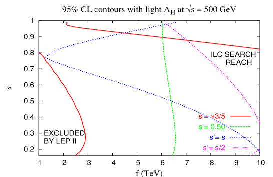
Figure 3: (Color online) LEP II exclusion region from $e^{+}e^{-}\rightarrow f\bar{f}$ and ILC search reach in the parameter space $(s,f)$ for different input values of $s^{\prime}$, and including the $A_{H}$ contribution. For $s^{\prime}=\sqrt{3/5}$ there are two lines of the same symbol/color, one on the boundary of the LEP II exclusion region, and one on the boundary of the ILC search reach region. For the other values of $s^{\prime}$ the curve shown is the boundary of the LEP II exclusion region, while the ILC search reach covers the entire parameter region shown.

For each value of $s^{\prime}$, the LEP II exclusion region and the ILC search reach are on the left of the corresponding contour. This is because as $f$ increases, the gauge boson masses (proportional to $f$) also increase (see Fig. 1) and the deviations in the $Z_{L}f\bar{f}$ couplings (proportional to $v^{2}/f^{2}$) decrease. For the ILC search reach boundary one would expect to see four contours at the upper right corner corresponding to the four different input values of $s^{\prime}$. However, there is only one visible contour, for $s^{\prime}=\sqrt{3/5}$, because in the other three cases, the search reach covers the entire parameter space shown in the figure.

As discussed above, the choice $s^{\prime}=\sqrt{3/5}$ corresponds to decoupling the $A_{H}$ from the fermion sector, as verified by the results shown in Eq. 8. In this case, the ILC search reach can be as low as $f\sim 2\,{\mathrm{TeV}}$ for large values of $s$. For other values of $s^{\prime}$, the search reach is greater than $f\sim 10\,{\mathrm{TeV}}$ for all values of $s$. We thus see how strongly the presence of the relatively-light $A_{H}$ can affect the phenomenology. For LEP II, the story is similar; the exclusion region for $s^{\prime}=\sqrt{3/5}$ is much smaller than for other values of $s^{\prime}$. This is because the observed deviation at $s^{\prime}=\sqrt{3/5}$ is solely due to the modification in the $Z_{L}f\bar{f}$ coupling and the presence of the $Z_{H}$, which is generally several times heavier than the $A_{H}$. For other values of $s^{\prime}$ the constraints on $f$ can be as high as $\sim$ 6 TeV. Overall, the LEP II exclusion regions have constraints on the parameter $f$ that are roughly consistent with those from precision measurements [1, 5, 6, 7, 8, 9].

As discussed in Sec. 2, we also examine the general behavior of models in which the $A_{H}$ is decoupled by taking $M_{A_{H}}\rightarrow\infty$ while letting all other quantities take on their usual values. The results in this case are presented in Fig. 4.

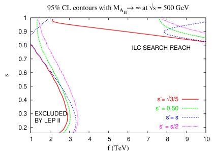
Figure 4: (Color online) LEP II exclusion region and ILC search reach as in Fig. 3, but with $M_{A_{H}}\rightarrow\infty$ .

It is not surprising that the $s^{\prime}=\sqrt{3/5}$ contours in Fig. 4 are exactly the same as in Fig. 3, since the $A_{H}$ is decoupled for this choice of $s^{\prime}$. For other values of $s^{\prime}$, the contours are very different in the two cases. The s dependence of the contours in Fig. 4 is easy to understand. The $Z_{H}f\bar{f}$ couplings go as $gc/s$, thus the ILC contours show that the search reach is higher for lower values of s. Similarly, for LEP II, the exclusion region extends farther out in $f$ for lower values of s. There is, however, a “turnover” for the LEP II exclusion region around $s\sim 0.3$ where the contours start moving towards lower $f$. This takes place because the mass $M_{Z_{H}}$ begins to increase (see Fig. 1) and the overall contribution from $Z_{H}$ to the observables starts to decrease as $s$ gets smaller.

With $M_{A_{H}}\rightarrow\infty$, the $s^{\prime}$-dependence of the $\chi^{2}$ is mostly due to the deviation in the $Z_{L}f\bar{f}$ couplings, since neither the $Z_{H}f\bar{f}$ couplings (see Eq. 8) nor $M_{Z_{H}}$ (see Eq. 6) are strongly dependent on $s^{\prime}$. This explains why there is less variation among the different contours in Fig. 4 than in Fig. 3. For values of $s$ close to $1$, however, the ILC contours for different values of $s^{\prime}$ begin to deviate from one another markedly. This $s^{\prime}$ dependence is due to the $s^{\prime}$-sensitive deviation of $A_{LR}$, as discussed in Sec. 2. This is confirmed by Fig. 5, which shows the relative contribution of the different observables to the $\chi^{2}$ at the ILC with $M_{A_{H}}\rightarrow\infty$ and $s=0.95$. Note that $A_{LR}$ for various final states dominates the $\chi^{2}$ where it is large.

The fact that the search reach is lowest for $s^{\prime}=\sqrt{3/5}$ then indicates that the deviations in the $Z_{L}f\bar{f}$ couplings are smallest for this parameter value. This coincidence arises because both $A_{H}$ and $Z_{L}$ are linear combinations of gauge eigenstates. $A_{H}$ to lowest order is just $B^{\prime}$, whose couplings to fermions vanish at $s^{\prime}=\sqrt{3/5}$. As the $s^{\prime}$-dependent terms in the deviation of the $Z_{L}f\bar{f}$ couplings arise from the $B^{\prime}$ admixture, they also vanish at this value. This is also confirmed by Fig. 5,

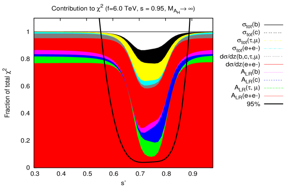
Figure 5: (Color online) Fractional contribution to the total $\chi^{2}$ for each $e^{+}e^{-}\rightarrow f\bar{f}$ observable at a $500\,{\mathrm{GeV}}$ ILC for fixed $(s,f)$. The labels on the legend go from top down in one-to-one correspondence with the shaded sections. For example, $A_{LR}(e^{+}e^{-})$ contributes $\sim$ 78% to the total $\chi^{2}$ at $s^{\prime}=0.4$. The line labeled “95%” is the total $\chi^{2}$/5.99. This means that the region $s^{\prime}\sim[0.55,0.9]$ where this line dips below 1 is outside the $\sqrt{s}=500\,{\mathrm{GeV}}$ ILC search reach.

which shows that the relative contribution of $A_{LR}$ and the total $\chi^{2}$ decrease around $s^{\prime}=\sqrt{3/5}$.

The search reach at a $\sqrt{s}=1\,{\mathrm{TeV}}$ ILC reaches to somewhat higher values of the parameter s, but has essentially the same reach for the parameter $f$ as the $\sqrt{s}=500\,{\mathrm{GeV}}$ machine. This is reasonable; as $s$ approaches unity, the contribution from the deviations in the $Z_{L}$ couplings dominates the search reach, and these contributions are not as important as the center of mass energy increases. The result is that the search reach is very simlar for both $\sqrt{s}=500$ GeV and 1 TeV. We will see later, however, that the $\sqrt{s}=1\,{\mathrm{TeV}}$ data can significantly improve the parameter determination.

Figure 3 and Fig. 4 show that the $\sqrt{s}=500\,{\mathrm{GeV}}$ ILC search reach in general covers most of the interesting parameter space where the Littlest Higgs models are relevant to the gauge hierarchy. Thus the $e^{+}e^{-}\rightarrow f\bar{f}$ process alone is an effective tool for investigating the Littlest Higgs model at a ILC.

It is important to compare the ILC search reach to that of the LHC. An ATLAS based analysis of the LHC search reach for the heavy gauge boson $Z_{H}$ of the Littlest Higgs model was computed in Ref. [17]. The resulting 5$\sigma$ contour for discovery of the $Z_{H}$ at the LHC is reproduced in Fig. 6 (where we have converted their results to our choices of parameters $f$ and $s$ for the axes). Fig. 6 also displays our results for the ILC (taking $M_{A_{H}}\rightarrow\infty$), where we have now employed a statistical significance of 5$\sigma$ rather than 95% to facilitate an equal comparison. We see that the ILC substantially extends the LHC search reach for $s\,\,\hbox to0.0pt{\raise 3.0pt\hbox{$<$}\hss}{\lower 3.0pt\hbox{$\sim$}}\,\,0.8$.

Figure 6: (Color online) Comparison of ILC and LHC search reach. The LHC data was taken from Fig. 8 of [17]. The search reach lies to the left of and underneath the contours.

3.2 Parameter Determination: sample fits

We have now determined the available parameter space accessible to the ILC and not already excluded by LEP II. It remains to ask, given the existence of an LH model with parameters in this accessible range, how accurately would the ILC be able to measure them? It is well-known [18, 19] that the ability to precisely measure the couplings of heavy gauge bosons is one of the fortes of the ILC.

We first discuss the capability of the LHC to determine the LH model parameters. Numerous studies [18, 20] have addressed the ability of the LHC to determine the couplings of new gauge bosons. The results of these studies show that while some model differentiation is possible for $Z^{\prime}$ bosons with masses $\,\,\hbox to0.0pt{\raise 3.0pt\hbox{$<$}\hss}{\lower 3.0pt\hbox{$\sim$}}\,\,2$  TeV, absolute determination of the $Z^{\prime}$ couplings is not possible. There are three main reasons for this: (i) the number of observables is limited in the hadron collider environment. The observables are the number of events (i.e., cross section times branching fraction), the forward-backward asymmetry, and the rapidity asymmetry) for leptonic final states only. Other final states are not detectable above background, ($t\bar{t}$ final states are a possible exception, but such events will be heavily smeared and thus not useful for a coupling analysis). (ii) The observables are convoluted with all contributing parton densities. (iii) The statistics are insufficient for $M_{Z^{\prime}}\mathrel{\mathchoice{\lower 3.01385pt\vbox{\halign{$\matth\displaystyle\hfil#\hfil$\cr>\crcr\sim\crcr}}}{\lower 3.01385pt\vbox{\halign{$\matth\textstyle\hfil#\hfil$\cr>\crcr\sim\crcr}}}{\lower 3.01385pt\vbox{\halign{$\matth\scriptstyle\hfil#\hfil$\cr>\crcr\sim\crcr}}}{\lower 3.01385pt\vbox{\halign{$\matth\scriptscriptstyle\hfil#\hfil$\cr>\crcr\sim\crcr}}}}2$ TeV. Here, in the case of the LH, our results show that LEP II essentially excludes the region $M_{Z_{H}}\,\,\hbox to0.0pt{\raise 3.0pt\hbox{$<$}\hss}{\lower 3.0pt\hbox{$\sim$}}\,\,2$  TeV, and thus we do not expect the LHC to contribute to the parameter extraction in any significant way. We note, however, that a very precise mass measurement for $Z_{H}$ will be obtained at the LHC.

To determine the accuracy of the parameter measurements, we perform some sample fits, using a $\chi$-square analysis similar to the one described in the preceding section. We use the same ILC observables as before. In some cases we also include data from a $\sqrt{s}=1\,{\mathrm{TeV}}$ run, for which we also take an integrated luminosity of ${\cal L}$= 500  ${\mathrm{fb}}^{-1}$. We note that we can exchange $M_{Z_{H}}$ for $f$, so we now take $M_{Z_{H}}$, $s$, and $s^{\prime}$ as our free parameters. We choose a generic data point $(s,s^{\prime},M_{Z_{H}})$ and use it to calculate the observables, which we then fluctuate according to statistical error. We assume that the Large Hadron Collider would have determined $M_{Z_{H}}$ relatively well, to the order of a few percent for $M_{Z_{H}}\,\,\hbox to0.0pt{\raise 3.0pt\hbox{$<$}\hss}{\lower 3.0pt\hbox{$\sim$}}\,\,5-6\,{\mathrm{TeV}}$; we thus fix $M_{Z_{H}}$ and perform a 2-variable fit to $s$ and $s^{\prime}$. Scanning the $s$-$s^{\prime}$ parameter space, we calculate the $\chi^{2}$ at every point. We find the minimum $\chi^{2}$ point; the 95% CL region surrounding it is the region for which the $\chi^{2}$ is less than this minimum $\chi^{2}$ plus 5.99.

Figure 7 shows the results of this fit for two sample data points in the contrived scenario with $M_{A_{H}}\rightarrow\infty$.

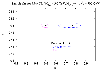
Figure 7: (Color online) 95% CL sample fits to the data points ($s=0.5$, $s^{\prime}=0.5$) and ($s=0.5$, $s^{\prime}=\sqrt{3/5}$), using $e^{+}e^{-}\rightarrow f\bar{f}$ observables at a 500  GeV ILC, taking $M_{Z_{H}}=3.0\,{\mathrm{TeV}}$ and $M_{A_{H}}\rightarrow\infty$.

For both of these points, the determination of $s$ is very accurate. This is due to the strong dependence of the $Z_{H}f\bar{f}$ couplings on $s$, as discussed in the previous section. The $s^{\prime}$ determination is worse than that for $s$ because of our choice $s=0.5$. At this value of $s$, the contributions from the $Z_{L}$ coupling deviations (which carry the $s^{\prime}$ dependence) are smaller than the $Z_{H}$ contributions. The reason the $s^{\prime}$ determination is better for $s^{\prime}=0.5$ than it is for $s^{\prime}=\sqrt{3/5}$ is that the $s^{\prime}$-dependent deviations in $g_{V_{Z_{L}f\bar{f}}}$ vanish for the latter value.

Figure 8 shows the results from a similar fit and illustrates how it can be improved with data from a higher-energy run with $\sqrt{s}=1\,{\mathrm{TeV}}$ at the ILC.

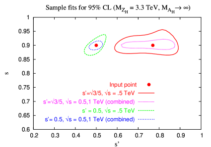
Figure 8: (Color online) Like Fig. 7 except $M_{Z_{H}}=3.3\,{\mathrm{TeV}}$ and the data points are ($s=0.9$, $s^{\prime}=0.5$) and ($s=0.9$, $s^{\prime}=\sqrt{3/5}$). Also shown for each point is an improved fit from adding data from a $\sqrt{s}=1\,{\mathrm{TeV}}$, ${\cal L}$= 500  ${\mathrm{fb}}^{-1}$run at the ILC.

Here, the $s$ determination is not much more accurate than the $s^{\prime}$ determination, as the $s^{\prime}$-independent $Z_{H}$ contributions no longer dominate the fit for $s=0.9$.

In Fig. 9 we show results from a fit with the full $A_{H}$ contributions.

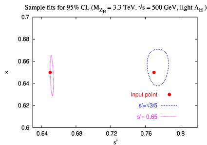
Figure 9: (Color online) Like Fig. 7, except $M_{Z_{H}}=3.3\,{\mathrm{TeV}}$ and the data points are ($s=0.65$, $s^{\prime}=0.65$) and ($s=0.65$, $s^{\prime}=\sqrt{3/5}$), and the full $M_{A_{H}}$ contributions are included.

Not surprisingly, the parameter determination is much more precise, as the $A_{H}$ contributions, when present, dominate the $\chi^{2}$. Since the $A_{H}$ couplings depend only on $s^{\prime}$, it is also no surprise that here the $s^{\prime}$ determination is in general much better than that for $s$.

If, for some reason, the LHC doesn’t provide a good measurement of $M_{Z_{H}}$, we would need to include that quantity, or equivalently $f$, in our fits to the data. In Fig. 10 we show the results where we have set $s^{\prime}=\sqrt{3/5}$ and we fit to $s$ and $f$. Note that for one of the data points, the allowed region doesn’t close. This highlights the importance of using both the LHC and the ILC to reliably determine the model parameters.

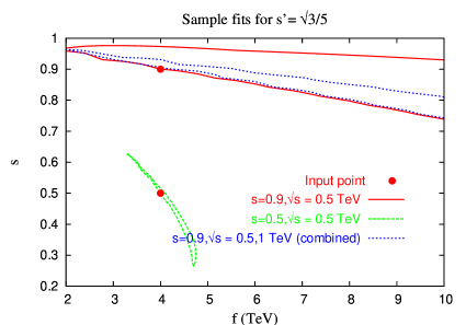
Figure 10: (Color online) Sample fits to the data points ($s=0.5$, $f=4\,{\mathrm{TeV}}$) and ($s=0.9$, $f=4\,{\mathrm{TeV}}$), taking $s^{\prime}=\sqrt{3/5}$. At the decoupling value of $s^{\prime}$, the ${A_{H}}$ does not contribute.

4 Parameter determination using $e^{+}e^{-}\rightarrow Z_{L}h$

In order to confirm that the LH model is the correct description of  TeV-scale physics, it is important to test the hallmark of the LH mechanism, namely that the Higgs mass quadratic divergences are canceled by new particles with the same spin as their SM counterparts. The proof lies in the measurement of the new particle couplings to the Higgs. Here we are concerned with the coupling of the heavy Z to the Higgs boson. This coupling can be tested via the process $e^{+}e^{-}\rightarrow Z_{L}h$. In the LH model, deviations of observables related to this process from their SM expectations come from three sources: the diagram with the $Z_{H}$ in the s-channel, the diagram with the $A_{H}$ in the s-channel, and the deviation of the $Z_{L}Z_{L}h$ coupling from its SM value.

In this section we repeat the analysis of Section 3, using the process $e^{+}e^{-}\rightarrow Z_{L}h$ and taking the total cross section as our observable with $m_{h}=120\,{\mathrm{GeV}}$. We assume that at a $\sqrt{s}=500\,{\mathrm{GeV}}$ ILC this cross section will be measured to an accuracy of 1.5% [15].

The cross section, including the effects of additional gauge bosons, can be written as

$$\sigma_{Z_{L}h}=\frac{|{\mathbf{k}}|}{8\pi\sqrt{s}}\left(1+\frac{|{\mathbf{k}}|^{2}}{3m_{Z}^{2}}\right)\sum_{ij}P_{ij}^{ss}[{g_{i}}_{Z_{L}h}{g_{j}}_{Z_{L}h}(v_{i}v_{j}+a_{i}a_{j})_{e}],$$ (17)

where $P_{ij}^{ss}$ was defined in Eq. 11. The sum runs over the participating gauge bosons in the s-channel: $Z_{L}$, $A_{H}$, and $Z_{H}$. Here, $|{\mathbf{k}}|$ is the magnitude of the 3-momentum of the outgoing $Z_{L}$, given by

$$|{\mathbf{k}}|=\frac{1}{2\sqrt{s}}\sqrt{(m_{H}^{2}-M_{Z_{L}}^{2})^{2}+s(s-2(M_{Z_{L}}^{2}+m_{H}^{2}))}.$$ (18)

The couplings $v_{i}$ and $a_{i}$ are the same as before–the axial and vector couplings of electrons to the $i$th gauge boson.

We carry out the $\chi$-square analysis as before. Figure 11 shows the ILC search reach in the LH parameter space,

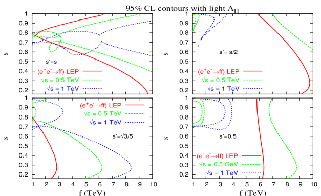
Figure 11: (Color online) LEP II exclusion region from $e^{+}e^{-}\rightarrow f\bar{f}$ and ILC search reach in the parameter space $(s,f)$ from the process $e^{+}e^{-}\rightarrow Z_{L}h$, for various values of $s^{\prime}$ and including the full $A_{H}$ contributions. For each value of $s^{\prime}$ there are three curves; one corresponds to the LEP II exclusion region, and the other two represent the ILC search reach region for $\sqrt{s}=500$ and $1000\,{\mathrm{GeV}}$, respectively, taking an integrated luminosity of 500  ${\mathrm{fb}}^{-1}$at each center-of-mass energy.

where each plot corresponds to a different choice of $s^{\prime}$. By comparing to Fig. 4 we note that $e^{+}e^{-}\rightarrow Z_{L}h$ gives a much poorer search reach than $e^{+}e^{-}\rightarrow f\bar{f}$. In particular, when $s^{\prime}$ is near the decoupling value $\sqrt{3/5}$ the LH model is generally indistinguishable from the SM. Well away from $s^{\prime}=\sqrt{3/5}$, as shown for $s^{\prime}=s/2$ and $s^{\prime}=0.5$, the search reach covers almost all of parameter space, except for regions of low $f$ where interference between the $A_{H}$ and $Z_{H}$ conspire to bring the cross section near its SM value. These regions, however, are ruled out by LEP.

In the case $s^{\prime}=s$, however, there are regions that exhibit similar interference effects and are not ruled out by LEP data. For example, consider the two data points $f=4.0\,{\mathrm{TeV}}$, $s=0.61$ with (a) $s^{\prime}=\sqrt{3/5}$ and (b) $s^{\prime}=0.61$. With $\sqrt{s}=500\,{\mathrm{GeV}}$, (b) is within the search reach while (a) is just outside the search reach. Figure 12 shows that at this value of $\sqrt{s}$, the deviation of the cross section from the SM is much greater for $s^{\prime}=0.61$ than for $s^{\prime}=\sqrt{3/5}$, since the $A_{H}$ decouples in the latter case. With $\sqrt{s}=1\,{\mathrm{TeV}}$, this behavior is reversed; point (a) is outside the search reach while (b) is within. At this value of $\sqrt{s}$ the interference between $A_{H}$ and $Z_{H}$ brings the cross section closer to the SM value when the $A_{H}$ contributes.

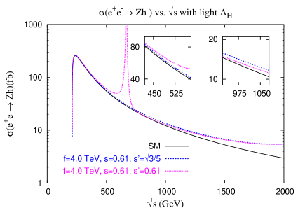
Figure 12: (Color online) The cross section for $e^{+}e^{-}\rightarrow\ Z_{L}h$ as a function of $\sqrt{s}$ for the SM and two different points in LH parameter space. The insets show the behavior near the expected ILC $\sqrt{s}$ values of $500\,{\mathrm{GeV}}$ and $1\,{\mathrm{TeV}}$. The resonance at about 700  GeV corresponds to the $A_{H}$.

Figure 13 shows the search reach obtainable with 500  ${\mathrm{fb}}^{-1}$at a $\sqrt{s}=500\,{\mathrm{GeV}}$ ILC, taking $M_{A_{H}}\rightarrow\infty$. Comparing to Fig. 3,

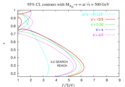
Figure 13: (Color online) The ILC search reach from the process $e^{+}e^{-}\rightarrow Z_{L}h$ for various values of $s^{\prime}$, taking $\sqrt{s}=500$ and $M_{A_{H}}\rightarrow\infty$. The LEP II exclusion region from $e^{+}e^{-}\rightarrow f\bar{f}$ is shown for $s^{\prime}=s/2$ (from Fig. 4) for comparison.

we see that the search reach here is much smaller than for $e^{+}e^{-}\rightarrow f\bar{f}$. Figure 14 displays the corresponding reach at $\sqrt{s}=1\,{\mathrm{TeV}}$ with 500  ${\mathrm{fb}}^{-1}$.

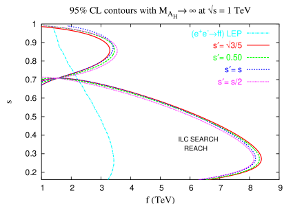
Figure 14: (Color online) Same as Fig. 13, but for $\sqrt{s}=1\,{\mathrm{TeV}}$.

In both cases, and for all choices of $s^{\prime}$, the search reach decreases markedly around $s=1/\sqrt{2}$. This is because the $Z_{L}Z_{H}H$ coupling vanishes at this value of $s$, as can be seen in Eq. 9. It is also interesting to note that the spread in the search reach as $s^{\prime}$ is varied is larger for $\sqrt{s}=500\,{\mathrm{GeV}}$ than it is for $1\,{\mathrm{TeV}}$. This can be understood if one notes that $\sqrt{s}=1\,{\mathrm{TeV}}$ is closer to the $Z_{H}$ pole (as $M_{Z_{H}}\simeq$ a few  TeV throughout the parameter space) than is $500\,{\mathrm{GeV}}$. Thus the deviation of $\sigma_{Zh}$ from its SM value at $\sqrt{s}=1\,{\mathrm{TeV}}$ is dominated by the presence of the $Z_{H}$, whose mass and couplings are essentially $s^{\prime}$-independent. At $\sqrt{s}=500\,{\mathrm{GeV}}$, the deviation of $\sigma_{Zh}$ has a more significant contribution from the deviation of the $e^{+}e^{-}Z_{L}$ coupling, which is strongly dependent on $s^{\prime}$ (see Fig. 2). For both values of $\sqrt{s}$, the sensitivity in the range of parameter space where $s\mathrel{\mathchoice{\lower 3.01385pt\vbox{\halign{$\matth\displaystyle\hfil#\hfil$\cr>\crcr\sim\crcr}}}{\lower 3.01385pt\vbox{\halign{$\matth\textstyle\hfil#\hfil$\cr>\crcr\sim\crcr}}}{\lower 3.01385pt\vbox{\halign{$\matth\scriptstyle\hfil#\hfil$\cr>\crcr\sim\crcr}}}{\lower 3.01385pt\vbox{\halign{$\matth\scriptscriptstyle\hfil#\hfil$\cr>\crcr\sim\crcr}}}}0.5$ does not reach beyond the general precision electroweak bound of $f\mathrel{\mathchoice{\lower 3.01385pt\vbox{\halign{$\matth\displaystyle\hfil#\hfil$\cr>\crcr\sim\crcr}}}{\lower 3.01385pt\vbox{\halign{$\matth\textstyle\hfil#\hfil$\cr>\crcr\sim\crcr}}}{\lower 3.01385pt\vbox{\halign{$\matth\scriptstyle\hfil#\hfil$\cr>\crcr\sim\crcr}}}{\lower 3.01385pt\vbox{\halign{$\matth\scriptscriptstyle\hfil#\hfil$\cr>\crcr\sim\crcr}}}}4\,{\mathrm{TeV}}$.

One could hope to improve the sensitivity by adding the measurement of the Higgs branching ratios as additional observables. It turns out, however, that the LH deviations of the branching ratios from their SM values are at most 1-2%, which is smaller than or equivalent to the experimental sensitivity at the ILC.

Lastly, we again compare the reach obtainable at the ILC from this process to that of the LHC in $pp\rightarrow Z_{H}Z_{L}+h$. We display the $5\sigma$ results from the ATLAS based analysis [17] of this process in the LH using the final state $\ell^{+}\ell^{-}b\bar{b}$ in Fig. 15. We also show our results, again adjusted for $5\sigma$ rather than $95\%$ statistical significance. This figure shows that the ILC overwhelms the capability of the LHC in this channel. In fact, our analysis of $e^{+}e^{-}\rightarrow f\bar{f}$ shows that for $s\,\,\hbox to0.0pt{\raise 3.0pt\hbox{$<$}\hss}{\lower 3.0pt\hbox{$\sim$}}\,\,0.8$ the LEP II results already exclude the possibility of the LHC observing the $Z_{L}+h$ decay of the $Z_{H}$.

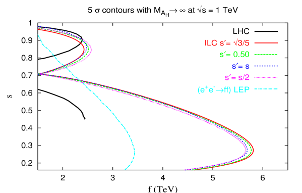
Figure 15: (Color online) Comparison of ILC and LHC search reach in the $Z_{H}\rightarrow Zh$ channel. The LHC curve was read from Fig. 22 of [17].

5 Summary

Little Higgs models provide an interesting mechanism for addressing the hierarchy problem. They contain a single light Higgs boson which is a pseudo-Goldstone boson with a small mass generated at the two-loop level. The quadratically divergent loop contributions to the mass of this Higgs are canceled by contributions from new particles appearing at the TeV scale. These cancelations take place between contributions from particles which have the same spin. Measurement of the couplings of these new particles to the light Higgs would verify the structure of these cancelations and establish the Little Higgs mechanism.

Here, we have investigated the extended gauge boson sector within these theories. Numerous Little Higgs models, based on various global symmetries, have been proposed. However, the existence of an enlarged gauge sector, with rather generic features, is endemic to all these scenarios. We choose to work in the framework of the simplest model of this type, known as the Littlest Higgs, based on an SU(5)/SO(5) nonlinear sigma model. This scenario contains the new heavy gauge bosons $W^{\pm}_{H}$, $Z_{H}$, and $A_{H}$ in addition to the SM gauge fields. The masses of these additional gauge bosons are expected to be of order the global symmetry breaking scale of $f\sim$ TeV. (It is expected that $f\,\,\hbox to0.0pt{\raise 3.0pt\hbox{$<$}\hss}{\lower 3.0pt\hbox{$\sim$}}\,\,10$ TeV in order for this scenario to be relevant to the hierarchy.) However, due to the group theory structure, the $A_{H}$ can be significantly lighter resulting in stringent constraints from precision electroweak data. Phenomenologically viable Littlest Higgs models must thus decouple the $A_{H}$ and we have examined two such approaches in our analysis. One, where we choose the model parameters such that the fermion couplings of the $A_{H}$ vanish, and another where we artificially take $M_{A_{H}}\rightarrow\infty$.

We study the effects of the new neutral gauge bosons in $e^{+}e^{-}$ annihilation. These particles can participate in $e^{+}e^{-}\rightarrow f\bar{f}$ and $e^{+}e^{-}\rightarrow Zh$ via s-channel exchange, and their effects can be felt indirectly for center of mass energies well below their masses. We find that fermion pair production is more sensitive to Little Higgs effects than $Zh$ associated production. We perform a thorough investigation of the model parameter space and find that observables at LEP II exclude the region $f\,\,\hbox to0.0pt{\raise 3.0pt\hbox{$<$}\hss}{\lower 3.0pt\hbox{$\sim$}}\,\,1-3$ TeV, which is consistent with the constraints obtained from precision electroweak data. The search reach of the proposed International Linear Collider, operating at $\sqrt{s}=500$ GeV, covers essentially the entire parameter region where this model is relevant to the hierarchy, i.e., $f\,\,\hbox to0.0pt{\raise 3.0pt\hbox{$<$}\hss}{\lower 3.0pt\hbox{$\sim$}}\,\,6-10$ TeV. In the case of a 1 TeV ILC, the search region probes slightly larger values of the mixing parameter $s$, but similar values of $f$.’

We have also demonstrated that once a signal is observed in these channels, accurate measurements of the couplings of the heavy gauge fields can be obtained from fermion pair production at the ILC. These couplings are related to the mixing angles in the extended gauge sector and we show that experiments at the ILC can determine the fundamental parameters of the theory. For illustration, we performed a fit to generated data for sample points in the Littlest Higgs parameter space, and found that the fundamental parameters can be determined to the precision of a few percent, provided that the LHC measures the mass of the heavy neutral gauge field. If information on the new boson masses is not available from the LHC, then the parameter determination at the ILC deteriorates. Additionally, the couplings of the extra gauge bosons to the light Higgs can separately be determined from $e^{+}e^{-}\rightarrow Zh$ for a significant region of the parameter space. This enables ILC experiments to test the consistency of the theory and verify the structure of the Higgs quadratic divergence cancelations.

In summary, we find that the ILC has the capability to discover the effects of the Littlest Higgs model over the entire theoretically interesting range of parameters, and to additionally determine the couplings of the heavy gauge bosons to the precision of a few percent.

Acknowledgments

We would like to thank T. Barklow, B. Lillie, H. Logan, M. Peskin, and T. Rizzo for helpful discussions. We thank G. Azuelos and G. Polesello for providing data for Fig. 6.

References

- [1] N. Arkani-Hamed, A. G. Cohen, E. Katz and A. E. Nelson, JHEP 0207, 034 (2002) [arXiv:hep-ph/0206021].
- [2] N. Arkani-Hamed, A. G. Cohen and H. Georgi, Phys. Lett. B 513, 232 (2001) [arXiv:hep-ph/0105239]; N. Arkani-Hamed, A. G. Cohen, E. Katz, A. E. Nelson, T. Gregoire and J. G. Wacker, JHEP 0208, 021 (2002) [arXiv:hep-ph/0206020]; I. Low, W. Skiba and D. Smith, Phys. Rev. D 66, 072001 (2002) [arXiv:hep-ph/0207243]; D. E. Kaplan and M. Schmaltz, JHEP 0310, 039 (2003) [arXiv:hep-ph/0302049]; S. Chang and J. G. Wacker, Phys. Rev. D 69, 035002 (2004) [arXiv:hep-ph/0303001].
- [3] W. Skiba and J. Terning, Phys. Rev. D 68, 075001 (2003) [arXiv:hep-ph/0305302]; S. Chang, JHEP 0312, 057 (2003) [arXiv:hep-ph/0306034].
- [4] E. Katz, J. y. Lee, A. E. Nelson and D. G. E. Walker, arXiv:hep-ph/0312287; D. E. Kaplan, M. Schmaltz and W. Skiba, Phys. Rev. D 70, 075009 (2004).
- [5] J. L. Hewett, F. J. Petriello and T. G. Rizzo, JHEP 0310, 062 (2003) [arXiv:hep-ph/0211218].
- [6] M. C. Chen and S. Dawson, Phys. Rev. D 70, 015003 (2004) [arXiv:hep-ph/0311032].
- [7] W. j. Huo and S. h. Zhu, Phys. Rev. D 68, 097301 (2003) [arXiv:hep-ph/0306029]; C. x. Yue and W. Wang, Nucl. Phys. B 683, 48 (2004) [arXiv:hep-ph/0401214].
- [8] C. Csaki, J. Hubisz, G. D. Kribs, P. Meade and J. Terning, Phys. Rev. D 68, 035009 (2003) [arXiv:hep-ph/0303236].
- [9] C. Csaki, J. Hubisz, G. D. Kribs, P. Meade and J. Terning, Phys. Rev. D 67, 115002 (2003) [arXiv:hep-ph/0211124].
- [10] E. Ros, Eur. Phys. J. C 33, S732 (2004); C. x. Yue, W. Wang and F. Zhang, arXiv:hep-ph/0409066; G. C. Cho and A. Omote, Phys. Rev. D 70, 057701 (2004) [arXiv:hep-ph/0408099]; S. C. Park and J. Song, Phys. Rev. D 69, 115010 (2004); J. J. Liu, W. G. Ma, G. Li, R. Y. Zhang and H. S. Hou, Phys. Rev. D 70, 015001 (2004) [arXiv:hep-ph/0404171]; G. Azuelos et al., arXiv:hep-ph/0402037; C. x. Yue, S. z. Wang and D. q. Yu, Phys. Rev. D 68, 115004 (2003) [arXiv:hep-ph/0309113]; Z. Sullivan, arXiv:hep-ph/0306266; G. Burdman, M. Perelstein and A. Pierce, Phys. Rev. Lett. 90, 241802 (2003) [Erratum-ibid. 92, 049903 (2004)] [arXiv:hep-ph/0212228]; W. Kilian and J. Reuter, Phys. Rev. D 70, 015004 (2004) [arXiv:hep-ph/0311095].
- [11] T. Han, H. E. Logan, B. McElrath and L. T. Wang, Phys. Rev. D 67, 095004 (2003) [arXiv:hep-ph/0301040]; T. Han, H. E. Logan and L. Wang, arXiv:hep-ph/0506313.
- [12] T. Gregoire, D. R. Smith and J. G. Wacker, Phys. Rev. D 69, 115008 (2004) [arXiv:hep-ph/0305275].
- [13] C. Kilic and R. Mahbubani, JHEP 0407, 013 (2004) [arXiv:hep-ph/0312053].
- [14] G. Abbiendi et al. [OPAL Collaboration], Eur. Phys. J. C 33, 173 (2004) [arXiv:hep-ex/0309053].
- [15] J. A. Aguilar-Saavedra et al. “Tesla Technical Design Report,” arXiv:hep-ph/0106315.
- [16] J. L. Hewett and T. G. Rizzo, Phys. Rept. 183, 193 (1989).
- [17] G. Azuelos et al., Eur. Phys. J. C 39S2, 13 (2005) [arXiv:hep-ph/0402037].
- [18] For review of the physics, see M. Cvetic and S. Godfrey, arXiv:hep-ph/9504216; T. G. Rizzo, eConf C960625, NEW136 (1996) [arXiv:hep-ph/9612440].
- [19] G. Weiglein et al. [LHC/LC Study Group], arXiv:hep-ph/0410364; J. A. Aguilar-Saavedra et al. [ECFA/DESY LC Physics Working Group], arXiv:hep-ph/0106315; T. Abe et al. [American Linear Collider Working Group], in Proc. of the APS/DPF/DPB Summer Study on the Future of Particle Physics (Snowmass 2001) ed. N. Graf, arXiv:hep-ex/0106057; S. Riemann. LC-TH-2001-007, Jan 2001; T. G. Rizzo, Phys. Rev. D 55, 5483 (1997) [arXiv:hep-ph/9612304]; J. L. Hewett and T. G. Rizzo, ANL-HEP-CP-91-90, Contribution to Proc. of Workshop on Physics and Experiments with Linear Colliders, Saariselka, Finland, Sep 9-14, 1991.
- [20] M. Dittmar, A. S. Nicollerat and A. Djouadi, Phys. Lett. B 583, 111 (2004) [arXiv:hep-ph/0307020]; F. del Aguila, M. Cvetic and P. Langacker, Phys. Rev. D 48, R969 (1993) [arXiv:hep-ph/9303299]; J. L. Hewett and T. G. Rizzo, Phys. Rev. D 45, 161 (1992).