Transverse Momentum Distribution Through
Soft-Gluon Resummation in Effective Field Theory

Abstract

We study resummation of transverse-momentum-related large logarithms generated from soft-gluon radiations in soft-collinear effective field theory. The anomalous dimensions of the effective quark and gluon currents, an important ingredient for the resummation, are calculated to two-loop order. The result at next-to-leading-log reproduces that obtained using the standard method for deep-inelastic scattering, Drell-Yan process, and Higgs production through gluon-gluon fusion. We comment on the extension of the calculation to next-to-next-to-leading logarithms.

I Introduction

Perturbative calculations of high-energy processes with widely separated scales often yield large logarithms involving the ratios of the scales, which shall be resummed to all orders to achieve reliable predictions. In processes like deep-inelastic scattering (DIS), Drell-Yan (DY) and the Higgs-boson production, multiple hard scales appear in a certain kinematical limit such as threshold production region Ste87 ; CatTre89 , and/or when a low transverse momentum DokDyaTro80 ; ParPet79 of the final states is measured. For the transverse momentum distribution, the rigorous theoretical study in QCD started with the classical work on semi-inclusive processes in $e^{+}e^{-}$ annihilation by Collins and Soper in ColSop81 , where a factorization was proved based on the transverse momentum-dependent (TMD) parton distributions and fragmentation functions ColSop81p . The resummation of TMD large logarithms was performed by solving the relevant energy evolution equation. This approach was later applied to the DY process in ColSopSte85 , where a general and systematic analysis of the factorization and resummation were performed. This latter procedure became known as “Collins-Soper-Sterman” (CSS) resummation formalism. The resummed formulas are used for many processes with the relevant coefficients extracted by comparing between the expansion of the resummed expressions and the fixed-order calculations davies . Although the factorization approach is sound and rigorous, it involves often quantities that are not manifestly gauge invariant. Moreover, the physics of the energy evolution does not seem transparent.

In this paper we pursue the same resummation from a different path. We exploit the fact that there are (at least) two well- separated hard scales which are naturally appropriate for an effective field-theoretic approach to perform the resummation. The recently proposed “soft-collinear-effective-theory” (SCET) SCET is useful here. Although it was originally applied for the study of heavy $B$ meson decays, it was later generalized to other high-energy processes SCET1 . Recently, this effective theory has been used to study the threshold resummation for the DIS structure function as $x\to 1$ in Man03 and for DY IdiJi05 . The resummation in the effective theory is performed by studying the anomalous dimensions $\gamma_{1}$ of the effective operators after performing matching between the full and effective theories. The exponentiated Sudakov form factor appears by running down the scale of the matching coefficient from the higher scale $\mu_{H}^{2}\sim Q^{2}$ down to the lower scale $\mu_{L}^{2}\sim\lambda Q^{2}$ ($\lambda\ll 1$).

A SCET study of transverse-momentum dependence for Higgs-boson production was initiated in Refs. Lics05 , where the authors work directly in momentum space, and the next-to-leading logarithmic result was deduced from a full QCD calculation. Here we consider the same resummation for the Drell-Yan process as well as the standard-model Higgs production at hadron colliders. Instead of working in the momentum space, we use the impact parameter space. Moreover we perform calculations directly in SCET.

In general, the resummation formula for these processes can be written in the following form, taking the DY process as an example ColSopSte85 ,

$$\frac{d\sigma}{dQ^{2}dydQ_{T}^{2}}=\sigma_{0}\left[\int\frac{d^{2}\vec{b}}{(2\pi)^{2}}e^{-i\vec{Q}_{T}\cdot\vec{b}}~{}W(b,Q^{2},x_{1},x_{2})+Y(Q_{T},Q^{2},x_{1},x_{2})\right]\ ,$$ (1)

where $\sigma_{0}=4\pi^{2}\alpha_{\rm em}^{2}/(9sQ^{2})$ represents the Born-level cross section for DY production. The variables used here are standard: $Q^{2}$ is the invariant mass of the DY pair; $Q_{T}$ is the observed transverse momentum relative to the beam axis; $y=(1/2)\ln(Q^{0}+Q^{3})/(Q^{0}-Q^{3})$ is the rapidity; $s=(P_{1}+P_{2})^{2}$ is the center-of-mass energy squared with $P_{i}$ the momentum of the incoming hadrons. The variable $x_{1}$ and $x_{2}$ are the equivalent parton fractions, $x_{1}=\sqrt{Q^{2}/s}~{}e^{y}$ and $x_{2}=\sqrt{Q^{2}/s}~{}e^{-y}$. The $W$ term contains the most singular contributions at small $Q_{T}$, resummed to all orders in perturbation theory. The second term $Y(Q_{T},Q^{2})$ represents the regular part of a fixed-order calculation for the cross section, which becomes important when the transverse momentum $Q_{T}$ is on the order of $\sqrt{Q^{2}}$.

The main result of our study can be summarized by the following formula for the $W$ term,

$$W(b,Q^{2},x_{1},x_{2}) = \sum_{qq^{\prime}}C^{2}(Q^{2},\alpha_{s}(Q^{2}))e^{-{\cal S}(Q^{2},~{}\mu_{L}^{2})}$$ (2)

$$\times\left(C_{q}\otimes q\right)(x_{1},b,Q,\mu_{L}^{2})\times\left(C_{q^{\prime}}\otimes{q^{\prime}}\right)(x_{2},b,Q,\mu_{L}^{2})\ ,$$

where $q$ and $q^{\prime}$ are the parton distributions and/or fragmentation functions related to the processes studied, and the notation $\otimes$ stands for convolution. Two matching coefficients appear in the above formula: one is $C(Q^{2},\alpha_{s}(Q^{2}))$ connecting between the matrix element of full QCD current and the effective theory analogue at the scale $Q^{2}$; the other is the coefficient function $C_{q}$ obtained by calculating the processes in SCET at a lower scale $\mu_{L}^{2}\sim Q_{T}^{2}$. The exponential suppression form factor arises from the anomalous dimension of the effective current in SCET,

$${\cal S}(Q^{2},\mu_{L}^{2})=\int_{\mu_{L}}^{Q}\frac{d\mu}{\mu}2\gamma_{1}(\mu^{2},\alpha_{s}(\mu^{2}))\$$ (3)

The anomalous dimension is identical for DIS and DY processes, and depends only on the effective theory operators. Moreover, the same $\gamma_{1}$ controls the threshold and the low transverse momentum resummations. The matching coefficient $C(Q^{2},\alpha_{s}(Q^{2}))$, on the other hand, is process dependent (but independent of threshold or transverse-momentum resummation). All the large double logarithms are included in the Sudakov form factor ${\cal S}$.

In the main body of the paper, we show how to get the above resummation formula using SCET. In Sec. II, we consider the resummation for the DY process in SCET. The anomalous dimensions of the effective current are calculated up to two-loop order. A comparison will be made with the CSS formalism. In Sec. III we will briefly discuss the extension of the formalism to the standard-model Higgs production. We conclude the paper in Sec. IV.

II Drell-Yan production at low $Q_{T}$ in SCET

In soft-collinear effective field theory, we consider Drell-Yan production with finite transverse momentum $Q_{T}$ in two steps, assuming $Q\gg Q_{T}\gg\Lambda_{\rm QCD}$. In the first step, one integrates out all loops with virtuality of order $Q$ to get an effective theory called SCET_I in which there are only collinear and soft modes. The collinear modes have virtuality of order $Q_{T}$. In the second step, one integrates out the collinear modes with virtuality $Q_{T}$. In this case, the theory is matched onto SCET_II which is just the ordinary QCD without external hard scales. The soft physics is now included in the parton distribution functions.

Let us consider the first step: integrating out modes of virtuality of order $Q$. At low $Q_{T}$, the most singular contribution in DY comes from the form-factor type of diagrams, in which the quark and antiquark first radiate soft gluons, followed by an annihilation vertex decorated with loop corrections. If the gluon radiations are attached to the loops, the soft gluon limit does not give rise to any infrared singularity, and hence diagrams yield higher-order contributions in $Q_{T}/Q$. Therefore, one needs to consider only the form-factor type of diagrams in studying the virtual corrections. To integrate out the hard modes (where all gluon momenta are of order $Q$– see, e.g., Zheng ) from the theory, we can match the full QCD current onto the (gauge invariant) SCET current Man03 ; IdiJi05 and the matching coefficient contains the hard contributions. By exploiting the non-renormalizability of the form factor, we write down a simple renormalization group equation from which we can extract the anomalous dimension of the effective current.

In the second step, we calculate the SCET cross section. One needs to compute only the real contributions since the virtual diagrams are scaleless in the effective theory and vanish in on-shell dimensional regularization (DR). At this stage the cross section obtained is the same as the one in full QCD taken to the relevant kinematical limit. This has been established at one-loop order in the threshold resummation for DIS and DY Man03 ; IdiJi05 . This will also be the case for DY in low transverse momentum limit.

Resumming the large logarithmic ratios is performed by considering the scale dependence of the matching coefficient, which is controlled by the anomalous dimension of the effective current. By running down the scale from $\mu_{H}^{2}\sim Q^{2}$ to the lower scale $\mu_{L}^{2}$, all the large logarithms exponentiate and give rise to the Sudakov form factor. In the following, we will demonstrate how this can be done systematically, providing a powerful tool for future studies. The basic lagrangian and Feynman rules for SCET can be found in Refs.SCET . In our calculation, we choose the two light-like vectors: $n=1/\sqrt{2}(1,0,0,-1)$ and $\bar{n}=1/\sqrt{2}(1,0,0,1)$. The matching is made between the full QCD current $\overline{\psi}\gamma_{\mu}\psi$ and the SCET_I current $\bar{\xi}_{n}W_{n}\gamma_{\mu}W_{\bar{n}}^{\dagger}\xi_{\bar{n}}$, where $\xi_{n,\bar{n}}$ are the collinear quark fields in SCET, and $W_{n,\bar{n}}$ are the collinear Wilson lines. The collinear Wilson lines appear as a requirement of the collinear gauge invariance in the SCET_I lagrangian. All calculations are performed in Feynman gauge and ${\overline{\rm MS}}$ scheme in $d=4-2\epsilon$. DR is employed to regularize both infrared (IR) as well as ultraviolet (UV) divergences.

II.1 Matching at scale $Q^{2}$ and anomalous dimension of SCET current at two loops

At the scale of $Q^{2}$, we need to consider only the virtual contributions to the quark form factor both in full QCD and the effective theory. The full QCD calculation of the quark form factor has so far been done up to two-loop order van . On the other hand, the virtual diagrams in the effective theory are scaleless, and the relevant form factors vanish in DR where the UV and IR divergences cancel out at every order in $\alpha_{s}$. Since the effective theory captures the IR behavior of the full theory (and the UV divergences are cancelled in both theories by respective counterterms), the matching coefficients for the effective theory operators will be obtained from the finite parts of the full QCD calculation. In the following, we will study the matching coefficients at one- and two-loop orders.

At one-loop order, the matching coefficient has been calculated ($C=\sum_{n}C^{(n)}$) Man03 ; IdiJi05 ,

$$C^{(1)}(\mu^{2},\alpha_{s}(\mu^{2}))=-\frac{\alpha_{s}(\mu^{2})C_{F}}{4\pi}\left[\ln^{2}\frac{Q^{2}}{\mu^{2}}-3\ln\frac{Q^{2}}{\mu^{2}}+8-\frac{7\pi^{2}}{6}\right]\ ,$$ (4)

where, throughout the paper, $\alpha_{s}$ is the renormalized running coupling constant.

From the above result, we can get the order-$\alpha_{s}$ anomalous dimension for the SCET current ($\gamma_{1}=\sum_{n}\gamma_{1}^{(n)}$),

$$\gamma_{1}^{(1)}=\frac{\alpha_{s}(\mu^{2})C_{F}}{\pi}\left[\ln\frac{Q^{2}}{\mu^{2}}-\frac{3}{2}\right]\$$ (5)

The matching coefficient satisfies the renormalization group equation,

$$\frac{\rm d}{\rm d\ln\mu}C(\mu,\alpha_{s}(\mu))=\gamma_{1}(\mu)C(\mu,\alpha_{s}(\mu))\$$ (6)

At the scale $\mu_{H}^{2}=Q^{2}$ we have,

$$C(Q^{2},\alpha_{s}(Q^{2}))=1+C^{(1)}=1-\frac{\alpha_{s}(Q^{2})}{2\pi}\left(4-\frac{7\pi^{2}}{12}\right)\$$ (7)

We note that the matching scale can also be chosen as $\mu_{H}^{2}=C_{2}^{2}Q^{2}$ with $C_{2}$ a constant of order unity. The $C_{2}$ dependence of the matching coefficient corresponds to the $C_{2}$ dependence in the CSS resummation ColSopSte85 . However, in order to minimize the logarithms in the matching coefficient $C(C_{2}^{2}Q^{2},\alpha_{s}(C_{2}^{2}Q^{2}))$, the best choice seems to be $C_{2}=1$.

To get the anomalous dimension at two-loop order, we need to calculate the matching coefficient up to the logarithmic term at the same order. From the quark form factor at two-loop order, we get the matching coefficient for DY process,

$$C^{(2)}(Q^{2},\mu^{2}) = \frac{\alpha_{s}^{2}}{(4\pi)^{2}}\left\{C_{F}^{2}\left[\frac{1}{2}\left(\ln^{2}\frac{-Q^{2}}{\mu^{2}}-3\ln\frac{-Q^{2}}{\mu^{2}}+8-\zeta(2)\right)^{2}\right.\right.$$ (8)

$$\left.+\left(24\zeta(3)+\frac{3}{2}-12\zeta(2)\right)\ln\frac{-Q^{2}}{\mu^{2}}\right]$$

$$\left.+N_{f}C_{F}\left[-\frac{2}{9}\ln^{3}\frac{-Q^{2}}{\mu^{2}}+\frac{19}{9}\ln^{2}\frac{-Q^{2}}{\mu^{2}}-\left(\frac{209}{27}-\frac{4}{3}\zeta(2)\right)\ln\frac{-Q^{2}}{\mu^{2}}\right]\right.$$

$$\left.+C_{A}C_{F}\left[\frac{11}{9}\ln^{3}\frac{-Q^{2}}{\mu^{2}}+\frac{1}{2}\left(4\zeta(2)-\frac{332}{9}\right)\ln^{2}\frac{-Q^{2}}{\mu^{2}}\right.\right.$$

$$\left.\left.-\left(\frac{2545}{54}+\frac{22}{3}\zeta(2)-26\zeta(3)\right)\ln\frac{-Q^{2}}{\mu^{2}}\right]\right\}+\cdots\$$

Here $\cdots$ stands for the constant terms which do not contribute to the anomalous dimension. The result contains an imaginary part because the DY form factor contains final-state rescattering. From the above result we can calculate the anomalous dimension at order $\alpha_{s}^{2}$. The expansion of Eq. (6) to order $\alpha_{s}^{2}$ gives

$$\frac{\partial}{\partial\ln\mu}C^{(2)}+\frac{\partial\alpha_{s}}{\partial\ln\mu}\frac{\partial}{\partial\alpha_{s}}C^{(1)} = \gamma_{1}^{(1)}C^{(1)}+\gamma_{1}^{(2)}C^{(0)}=\gamma_{1}^{(1)}C^{(1)}+\gamma_{1}^{(2)}\ .$$ (9)

The running of the strong coupling constant $\alpha_{s}(\mu)$ is

$$\frac{\partial}{\partial\ln\mu}\alpha_{s}=-2\beta_{s}\alpha_{s}^{2}\ ,$$ (10)

where $\beta_{s}$ has the following expansion,

$$\beta_{s}=\frac{1}{4\pi}\left[\beta_{0}+\frac{\alpha_{s}}{4\pi}\beta_{1}+\cdots\right]\ .$$ (11)

$\beta_{0}$ and $\beta_{1}$ are defined as

$$\beta_{0}=\frac{11}{3}C_{A}-\frac{2}{3}N_{f},~{}~{}~{}\beta_{1}=\frac{34}{3}C_{A}^{2}-4N_{f}T_{F}C_{F}-\frac{20}{3}N_{f}T_{F}C_{A}\ ,$$ (12)

where $N_{f}$ is the number of light flavors, $C_{A}=N_{C}$ with $N_{C}$ the number of colors, $C_{F}=(N_{C}^{2}-1)/2N_{C}$, $T_{F}=1/2$. Using the above formulas, we get the anomalous dimension at two-loop order,

$$\gamma_{1}^{(2)} = \left(\frac{\alpha_{s}}{\pi}\right)^{2}\left\{\left[\left(\frac{67}{36}-\frac{\pi^{2}}{12}\right)C_{A}-\frac{5}{18}N_{f}\right]C_{F}\ln\frac{Q^{2}}{\mu^{2}}\right.$$ (13)

$$~{}~{}~{}~{}+\left(\frac{13}{4}\zeta(3)-\frac{961}{16\times 27}-\frac{11}{48}\pi^{2}\right)C_{A}C_{F}$$

$$~{}~{}~{}~{}+\left(\frac{\pi^{2}}{24}+\frac{65}{8\times 27}\right)N_{f}C_{F}$$

$$~{}~{}~{}~{}\left.+\left(\frac{\pi^{2}}{4}-\frac{3}{16}-3\zeta(3)\right)C_{F}^{2}\right\}\ .$$

Using the notation of vanHiggs , we can write

$$\gamma_{1}^{(2)}=\frac{\alpha_{s}^{2}}{(4\pi)^{2}}\left(\frac{1}{2}\gamma_{Kqq}^{(1)}\ln\frac{Q^{2}}{\mu^{2}}-\gamma_{qq}^{(1)}-2f_{q2}^{(1)}\right)\$$ (14)

where

$$\gamma_{Kqq}^{(1)}=16C_{F}K,~{}~{}~{}K=C_{A}\left(\frac{67}{18}-\zeta(2)\right)-\frac{10}{9}N_{f}T_{F}\$$ (15)

is proportional to the anomalous dimension of a Wilson line cusp, and

$$\gamma_{qq}^{(1)} = C_{F}^{2}\left(3-24\zeta(2)+48\zeta(3)\right)+C_{A}C_{F}\left(\frac{17}{3}+\frac{88}{3}\zeta(2)-24\zeta(3)\right)$$ (16)

$$+N_{f}T_{F}C_{F}\left(-\frac{4}{3}-\frac{32}{3}\zeta(2)\right)$$

is proportional to the coefficient of $\delta(1-x)$ in the quark splitting function, and finally

$$f_{q2}^{(1)}=C_{F}\left[-2\beta_{0}\zeta(2)+C_{A}\left(\frac{404}{27}-14\zeta(3)\right)+N_{f}T_{F}C_{F}\left(-\frac{112}{27}\right)\right]\ .$$ (17)

The above calculation can be repeated for the DIS process and the same anomalous dimension is obtained.

II.2 Matching at scale $\mu_{L}^{2}$

To perform matching at the lower scale $\mu_{L}^{2}\ll Q^{2}$ we calculate the cross section in SCET_I and match it to a product of quark distributions. From the result we can extract the coefficient functions. The parton distributions in SCET_II are the same as those in full QCD Man03 ; IdiJi05 . Below the scale $Q^{2}$, the hard modes have been integrated out, and have been taken into account by the matching condition at $Q^{2}$. Therefore, the calculation of the cross section at $\mu_{L}^{2}$ is performed with SCET_I diagrams, including both virtual and real contributions. As mentioned earlier the virtual diagrams in SCET are scaleless and vanish in pure DR. As such one can ignore them, but the counterterm for the effective current must be taken into account. This is equivalent to taking the UV-subtracted contribution from the virtual diagrams. The counterterm has been calculated in Man03 ,

$${\rm c.t.} = \frac{\alpha_{s}}{2\pi}C_{F}\left[-\frac{1}{\epsilon^{2}}-\frac{3}{2\epsilon}-\frac{1}{\epsilon}\ln\frac{\mu^{2}}{Q^{2}}\right]\ ,$$ (18)

where $\mu^{2}$ will be taken as $\mu_{L}^{2}$.

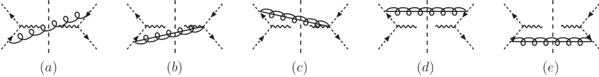
Figure 1: Non-vanishing Feynman diagrams contributing to Drell-Yan production in the soft-collinear-effective theory: (a) for the soft gluon radiation; (b)-(e) for $n$ and $\bar{n}$ collinear gluon radiations. The mirror diagrams of (a-c) are not shown here but are included in the results.

The real contribution contains collinear and soft gluon radiation diagrams. Some of these diagrams are identically zero because of $n^{2}=0$ or $\bar{n}^{2}=0$, or because of the equation of motion for the external collinear (anti-)quark. The non-vanishing diagrams are shown in Fig. 1, including soft-gluon interference contribution, $n$ and $\bar{n}$ collinear gluon radiations and their interferences. The contribution from Fig. 1(a) is, including that from the mirror diagram,

$$\frac{d^{3}\sigma^{(1)}}{d^{2}Q_{T}dy}|_{\rm fig.1(a)}=\sigma_{0}\frac{\alpha_{s}C_{F}}{\pi^{2}}\frac{1}{Q_{T}^{2}}\left[-\frac{\delta(x_{2}-1)}{(1-x_{1})_{+}}-\frac{\delta(x_{1}-1)}{(1-x_{2})_{+}}-\delta(x_{1}-1)\delta(x_{2}-1)\ln\frac{Q^{2}}{Q_{T}^{2}}\right]\$$ (19)

Fig.1(b) represents the interference between the $\bar{n}$-collinear gluon radiation with collinear expansion of the current operator, and its contribution is,

$$\frac{d^{3}\sigma^{(1)}}{d^{2}Q_{T}dy}|_{\rm fig.1(b)}=\sigma_{0}\frac{\alpha_{s}C_{F}}{\pi^{2}}\frac{1}{Q_{T}^{2}}\left[\frac{x_{1}\delta(x_{2}-1)}{(1-x_{1})_{+}}+\frac{\delta(x_{1}-1)}{(1-x_{2})_{+}}+\delta(x_{1}-1)\delta(x_{2}-1)\ln\frac{Q^{2}}{Q_{T}^{2}}\right]\$$ (20)

while Fig.1(c) for the $n$-collinear gluon radiation yields,

$$\frac{d^{3}\sigma^{(1)}}{d^{2}Q_{T}dy}|_{\rm fig.1(c)}=\sigma_{0}\frac{\alpha_{s}C_{F}}{\pi^{2}}\frac{1}{Q_{T}^{2}}\left[\frac{x_{2}\delta(x_{1}-1)}{(1-x_{2})_{+}}+\frac{\delta(x_{2}-1)}{(1-x_{1})_{+}}+\delta(x_{1}-1)\delta(x_{2}-1)\ln\frac{Q^{2}}{Q_{T}^{2}}\right]\$$ (21)

Figs. 1(d) and (e) stand for the $n$ and $\bar{n}$ collinear gluon radiations, respectively, and their sum is,

$$\frac{d^{3}\sigma^{(1)}}{d^{2}Q_{T}dy}|_{\rm fig.1(de)}=\sigma_{0}\frac{\alpha_{s}C_{F}}{2\pi^{2}}\frac{1}{Q_{T}^{2}}\left(1-\epsilon\right)\left[(1-x_{1})\delta(x_{2}-1)+(1-x_{2})\delta(x_{1}-1)\right]\ .$$ (22)

The sum of the above contributions reproduces the result of the full QCD calculation in the limit of low transverse momentum (see, e.g., JiMaYu04 ).

From the above, the real contribution contains soft divergences (i.e, when $Q_{\perp}^{2}\rightarrow 0$), which will be cancelled by the virtual contribution. To see this cancellation explicitly, we Fourier-transform the cross section from the transverse momentum space into the impact parameter $b$-space. The result is $W(b,Q^{2},\mu_{L}^{2})$ in SCET, including real and virtual contributions (the contourterm, Eq. (18)),

$$W(b,Q^{2},\mu_{L}^{2},x_{1},x_{2})$$

$$=\delta(x_{1}-1)\delta(x_{2}-1)+\frac{\alpha_{s}C_{F}}{2\pi}\left[{\cal P}_{q/q}(x_{1})\delta(x_{2}-1)+(x_{1}\leftrightarrow x_{2})\right]\left(-\frac{1}{\epsilon}-\gamma_{E}+\ln\frac{4}{4\pi\mu_{L}^{2}b^{2}}\right)$$

$$+\frac{\alpha_{s}C_{F}}{2\pi}\left[(1-x_{1})\delta(x_{2}-1)+(1-x_{2})\delta(x_{1}-1)\right]$$

$$-\frac{\alpha_{s}C_{F}}{2\pi}\delta(x_{1}-1)\delta(x_{2}-1)\left[\ln^{2}\left(\frac{\mu_{L}^{2}b^{2}}{4}e^{2\gamma_{E}-\frac{3}{2}}\right)+2\ln\frac{Q^{2}}{\mu_{L}^{2}}\ln\left(\frac{\mu_{L}^{2}b^{2}}{4}e^{2\gamma_{E}}\right)-\frac{9}{4}+\frac{\pi^{2}}{6}\right]\ ,$$

(23)

where ${\cal P}_{q/q}$ is the one-loop quark splitting function,

$${\cal P}_{q/q}(x)=\left(\frac{1+x^{2}}{1-x}\right)_{+}\$$ (24)

The soft divergences in $W(b,Q^{2},\mu_{L}^{2})$ have been cancelled. There is, however, the collinear divergence left which can be absorbed into the quark distribution at one-loop order. The cross section depends on the ultraviolet scale $\mu_{L}^{2}$. It is somewhat surprising that the above result also depends on $\ln Q^{2}$, but this is expected from the kinematical constraints of the process.

In order to eliminate the large logarithms in the coefficient function, the best choice for the scale $\mu_{L}$ is $\mu_{L}^{2}=C_{1}^{2}/b^{2}$ with $C_{1}=2e^{-\gamma_{E}}$. In addition, $W(b,Q^{2},\mu_{L}^{2})$ no longer depends on $Q^{2}$ at this order. This, however, may not be true at higher orders because one cannot eliminate all $\ln Q^{2}$ by making a single choice of $\mu_{L}^{2}$. Considering the quark distribution at one-loop order, we can cast Eq. (23) into the form,

$$W(b,\mu_{L}^{2}=C_{1}^{2}/b^{2},x_{1},x_{2})=C_{q}(b,x_{1},\mu_{L}^{2})\otimes q(x,\mu_{L}^{2})C_{\bar{q}}(b,x_{2},\mu_{L}^{2})\otimes\bar{q}(x,\mu_{L}^{2})\ ,$$ (25)

where $C_{q}$ reads

$$C_{q}(b,x,\mu_{L}^{2}) = \delta(1-x)+\frac{\alpha_{s}C_{F}}{2\pi}\left[(1-x)-\delta(x-1)\left(\frac{\pi^{2}}{12}\right)\right]\ ,$$ (26)

and $C_{\bar{q}}=C_{q}$. Note that we have set the quark charge $e_{q}$ to 1.

II.3 Resummation and comparison with conventional approach

The final result for $W(b,Q^{2})$ is a combination of the factors we have calculated in the previous subsections, and as have been advertised in the introduction Man03 ; IdiJi05 ,

$$W(b,Q^{2},x_{1},x_{2})=\sum_{q\bar{q}}C^{2}(Q^{2},\alpha_{s}(Q^{2}))e^{-{\cal S}(Q^{2},~{}\mu_{L}^{2})}\left(C_{q}\otimes q\right)(x_{1},b,Q^{2},\mu_{L}^{2})\left(C_{\bar{q}}\otimes\bar{q}\right)(x_{2},b,Q^{2},\mu_{L}^{2})\ ,$$ (27)

where the exponential suppression factor can be calculated from the anomalous dimension calculated in Sec. IIA,

$${\cal S}=\int_{\mu_{L}}^{Q}\frac{d\mu}{\mu}2\gamma_{1}(Q^{2},\mu^{2})=\int_{\mu_{L}^{2}}^{Q^{2}}\frac{d\mu^{2}}{\mu^{2}}\left[A\ln\frac{Q^{2}}{\mu^{2}}+B\right]\ .$$ (28)

Here $A$ and $B$ are the single logarithmic and constant terms in the anomalous dimension $\gamma_{1}$, respectively. The separation of the anomalous dimension into a sum of these two terms holds to any order in perturbation theory. The Sudakov form factor comes from the running of the matching coefficient $C(Q^{2},\mu^{2})$ from $\mu^{2}=Q^{2}$ down to the scale of $\mu_{L}^{2}$ which can be taken as $C_{1}^{2}/b^{2}$.

The above is the final resummation result in the effective theory. $A$ and $B$ coefficient functions can be expanded as a series of $\alpha_{s}$: $A=\sum_{i=1}A^{(i)}\left(\frac{\alpha_{s}}{\pi}\right)^{i}$ and $B=\sum_{i=1}B^{(i)}\left(\frac{\alpha_{s}}{\pi}\right)^{i}$. From the result in Sec. IIA, we have the first two terms of these expansions,

$$A^{(1)} = C_{F}\ ,$$

$$B^{(1)} = -\frac{3}{2}C_{F}\ ,$$

$$A^{(2)} = \left[\left(\frac{67}{36}-\frac{\pi^{2}}{12}\right)C_{A}-\frac{5}{18}N_{f}\right]C_{F}\ ,$$

$$B^{(2)} = \left(\frac{13}{4}\zeta(3)-\frac{961}{16\times 27}-\frac{11}{48}\pi^{2}\right)C_{A}C_{F}+\left(\frac{\pi^{2}}{24}+\frac{65}{8\times 27}\right)N_{f}C_{F}$$ (29)

$$+\left(\frac{\pi^{2}}{4}-\frac{3}{16}-3\zeta(3)\right)C_{F}^{2}\ .$$

In the present formulation, the summation of leading logarithms (LL) involves $A^{(1)}$; that of next-to-leading (NLL) logarithms involves $A^{(2)}$ and $B^{(1)}$; and that of next-to-next-to-leading logarithms (NNLL) involves $A^{(3)}$, $B^{(2)}$, one-loop $C_{q}$, and part of the two-loop $C_{q}$ [we write $C_{q}=\sum_{n}C_{q}^{(n)}$].

To compare with the CSS approach we follow the procedure outlined in CatDefGra01 by absorbing the factor $C(Q^{2},\alpha_{s}(Q^{2}))$ into $B$ and $C$ functions, for example, up to order $\alpha_{s}$,

$$C_{q/\rm CSS}^{(1)}(x) = C_{q}^{(1)}(x)+\delta(1-x)\frac{1}{2}\left(C(Q^{2},\alpha_{s}(Q^{2}))\right)^{2}\ ,$$

$$B_{\rm CSS}^{(2)} = B^{(2)}+\beta_{0}\frac{\alpha_{s}}{4\pi}\left(C(Q^{2},\alpha_{s}(Q^{2}))\right)^{2}\$$ (30)

At two-loop level and beyond, one has to shuffle the $\ln Q^{2}$-dependent part of $C_{q}$ into $B_{\rm CSS}$ as well. In this way, we get the CSS resummation formula as,

$$W(Q^{2},b^{2})=e^{-{\cal S}_{\rm sud}}\left(C_{q/\rm CSS}\otimes q\right)(x_{1},b,\mu_{L}^{2})\left(C_{\bar{q}/\rm CSS}\otimes\bar{q}\right)(x_{2},b,\mu_{L}^{2})\ ,$$ (31)

with

$${\cal S}_{\rm sud}=\int_{\mu_{L}^{2}}^{Q^{2}}\frac{d\mu^{2}}{\mu^{2}}\left[A_{\rm CSS}\ln\frac{Q^{2}}{\mu^{2}}+B_{\rm CSS}\right]\ .$$ (32)

$A_{\rm CSS}$ will be the same as our $A$ functions, as does $B^{(1)}$. For $C_{q/\rm CSS}$, we have

$$C_{q/\rm CSS}^{(1)}(b,x,\mu_{L}^{2}) = \frac{\alpha_{s}C_{F}}{2\pi}\left[(1-x)-\delta(x-1)\left(4-\frac{\pi^{2}}{2}\right)\right]\ .$$ (33)

Comparing with the results in ColSopSte85 , we find that we can reproduce the $A^{(1)}_{\rm CSS}$, $A^{(2)}_{\rm CSS}$, $B^{(1)}_{\rm CSS}$, $C^{(1)}_{\rm CSS}$, which are all the coefficients and functions needed for resummation at NLL order. $B^{(2)}_{\rm CSS}$ will be needed to resum NNLL. However, to fully achieve NNLL resummation we need to calculate the matching coefficient at the lower scale up to order $\alpha_{s}^{2}$ in SCET DefGra01 . We leave this to a future publication.

Following the above, the resummation for SIDIS can be performed similarly. As we stated earlier, the anomalous dimension will be the same. The only difference is the process-dependent matching coefficients at $Q^{2}$ and $\mu_{L}^{2}$ in the resummation formula. For DIS, one has the one-loop result,

$$C_{\rm DIS}^{(1)}(Q^{2},\alpha_{s}(Q^{2}))=-\frac{\alpha_{s}}{2\pi}\left[4-\frac{\pi^{2}}{12}\right]\ ,$$ (34)

which leads to the result for the $C_{q/\rm CSS}^{(1)}$ in DIS,

$$C_{q/\rm CSS}^{(1)} = \frac{\alpha_{s}C_{F}}{2\pi}\left[(1-x)-4\delta(x-1)\right]\ .$$ (35)

These results agree with those from the conventional resummation approach Nadolsky:1999kb .

III Standard-model Higgs production

Transverse-momentum dependence of the Standard Model Higgs production can also be studied through resummation of large double logarithms. Higgs production, for a large range of Higgs mass, can be described by an effective action with a pointlike coupling between the Higgs particle and gluon fields. The effective coupling is of course scale dependent, balancing the renormalization dependence of the composite operator. In general, this effective lagrangian can be written as vanHiggs ,

$${\cal L}_{Hgg}=C_{EW}(M_{t})C_{T}(M_{t},\mu)HF^{a}_{\mu\nu}F^{a\mu\nu}\ ,$$ (36)

where $H$ is the scalar Higgs field and $F^{a}_{\mu\nu}$ is the gluon field strength tensor. $C_{EW}$ represents the electroweak coupling coefficient from the heavy-top-quark loop calculation, while $C_{T}$ comes from the strong interaction radiative corrections. The coefficient $C_{T}$ will depend, in general, on the top quark mass and the renormalization scale $\mu$. To our interest, we quote at two-loop HiggsOneloop ; Chetyrkin:1997iv ,

$$C_{T}(M_{t},\mu) = \frac{\alpha_{s}(\mu)}{4\pi}\left\{1+\frac{\alpha_{s}(\mu)}{4\pi}\left(5C_{A}-3C_{F}\right)\right.$$ (37)

$$\left.+\frac{\alpha_{s}^{2}(\mu)}{(4\pi)^{2}}\left[\ln\frac{\mu^{2}}{M_{t}^{2}}\left(7C_{A}^{2}-11C_{A}C_{F}+8N_{f}T_{F}C_{F}\right)+\cdots\right]\right\}\ .$$

Here we have omitted the constant terms of order $\alpha_{s}^{2}$ because they do not contribute to the renormalization group running at two-loop order.

In SCET, the Higgs production cross section can be calculated from its coupling with the collinear gluon fields,

$${\cal L}_{H-SCET}=C(M_{H},\mu)H{\cal F}^{a}_{n\mu\nu}{\cal F}^{a\bar{n}\mu\nu}\ ,$$ (38)

where ${\cal F}^{a}_{n,\bar{n}\mu\nu}$ represent the $n$ and $\bar{n}$ collinear gluon field strength tensors in SCET SCET . $C(M_{H},\mu)$ is the matching coefficient which contains the coupling of Higgs boson to gluons in full QCD,

$$C(M_{H},\mu)=C_{EW}(M_{t})C_{T}(M_{t},\mu)C_{G}(M_{H},\mu)\ .$$ (39)

The last factor comes from matching between operator $HF^{a}_{\mu\nu}F^{a\mu\nu}$ in full QCD and $H{\cal F}^{a}_{n\mu\nu}{\cal F}^{a\bar{n}\mu\nu}$ in SCET. Because $C_{EW}$ has no QCD effects, we will not discuss it further in this paper. $C_{T}$ and $C_{G}$ contain the QCD evolution effects, and thus the anomalous dimension of the SCET operator $H{\cal F}^{a}_{n\mu\nu}{\cal F}^{a\bar{n}\mu\nu}$ is the sum of the two:

$$\gamma_{1}=\gamma_{T}+\gamma_{G}\ ,$$ (40)

where $\gamma_{T}$ and $\gamma_{G}$ are defined as

$$\gamma_{T} = \frac{d\ln C_{T}(\mu)}{d\ln\mu}\ ,$$

$$\gamma_{G} = \frac{d\ln C_{G}(\mu)}{d\ln\mu}\ .$$ (41)

From Eq. (37), it is easy to show that

$$\gamma_{T} = -2\beta_{0}\frac{\alpha_{s}}{4\pi}+\frac{\alpha_{s}^{2}}{(4\pi)^{2}}\left[-2\beta_{1}-2\beta_{0}(5C_{A}-3C_{F})\right.$$ (42)

$$\left.+2\left(7C_{A}^{2}-11C_{A}C_{F}+8N_{f}T_{F}C_{F}\right)\right]\ ,$$

up to two-loop order. To calculate $\gamma_{G}$, we follow the calculation for the Drell-Yan process in the previous section. Using the gluon form factor in vanHiggs ; Har00 , we get the relevant anomalous dimension,

$$\gamma_{G} = \frac{\alpha_{s}}{\pi}C_{A}\ln\frac{M_{H}^{2}}{\mu^{2}}$$ (43)

$$+\frac{\alpha_{s}^{2}}{(4\pi)^{2}}\left[\frac{1}{2}C_{A}K\ln\frac{M_{H}^{2}}{\mu^{2}}-\gamma_{gg}^{(1)}-2f_{g2}^{(1)}+4\beta_{1}\right]\ ,$$

where $f_{g2}^{(1)}$ can be obtained from the above $f_{q2}^{(1)}$ by color-factor exchange ($C_{A}\leftrightarrow C_{F}$) vanHiggs . The anomalous dimension $\gamma_{gg}^{(1)}$

$$\gamma_{gg}^{(1)}=C_{A}^{2}\left(\frac{64}{3}+24\zeta(3)\right)-\frac{32}{3}N_{f}T_{F}C_{A}-8N_{f}T_{F}C_{F}\ ,$$ (44)

is proportional to $\delta(1-x)$ in the gluon splitting function. $\beta_{1}$ is the two-loop beta function defined before.

Including the matching at lower scale $\mu_{L}$, the result for Higgs production $W(b,M_{H}^{2},x_{1},x_{2})$ at low transverse momentum can be written as,

$$W(M_{H}^{2},b)=C^{2}_{H}(M_{H}^{2},\alpha_{s}(M_{H}^{2}))e^{-{\cal S}}\left(C_{g}\otimes g\right)(x_{1},b,\mu_{L}^{2})\left(C_{g}\otimes g\right)(x_{2},b,\mu_{L}^{2})\ ,$$ (45)

where $C_{EW}$ and the leading factor in $C_{T}$ have been absorbed in the Born cross section, and the remainder $C_{H}$ is

$$C_{H}(M_{H}^{2},\alpha_{s}(M_{H}^{2}))=1+\frac{\alpha_{s}(M_{H}^{2})}{4\pi}\left[5C_{A}-3C_{F}+C_{A}\left(\zeta(2)+\pi^{2}\right)\right]\ ,$$ (46)

up to one-loop order. The Sudakov suppression form factor has the same form as that for DY, and the expansions of the $A$ and $B$ are,

$$A_{H}^{(1)} = C_{A}$$

$$B_{H}^{(1)} = -\frac{1}{2}\beta_{0}$$

$$A_{H}^{(2)} = C_{A}K$$

$$B_{H}^{(2)} = -\frac{1}{16}\left[\gamma_{gg}^{(1)}+2f_{g2}^{(1)}+2\beta_{0}\left(5C_{A}-3C_{F}\right)-2\beta_{1}\right.$$ (47)

$$\left.-2\left(7C_{A}^{2}-11C_{A}C_{F}+8N_{f}T_{F}C_{F}\right)\right]\$$

With these results we can reproduce the conventional resummation for Higgs-boson production at NLL order DefGra01 .

The coefficient $C_{g}$ to one-loop order is calculated from the matching at the scale of $\mu_{L}$, with real and virtual contributions. It is needed for resummation at NLL. The result is

$$C_{g}(b,x,\mu_{L}^{2}) = \delta(1-x)+\frac{\alpha_{s}C_{A}}{2\pi}\delta(x-1)\left(-\frac{\pi^{2}}{12}\right)\ ,$$ (48)

where we have chosen $\mu_{L}=C_{1}/b$ with $C_{1}=2e^{-\gamma_{E}}$ to eliminate the large logarithms. The corresponding coefficient for CSS resummation is

$$C_{g/\rm CSS}(b,x,\mu_{L}^{2})=\delta(1-x)+\frac{\alpha_{s}C_{A}}{4\pi}\delta(1-x)\left[(5+\pi^{2})C_{A}-3C_{F}\right]$$ (49)

which is consistent with DefGra01 .

IV Conclusion

In this paper, we demonstrated how to perform resummation of large double logarithms in hard processes involving low transverse momentum in the framework of effective field theory. The newly-discovered theory, SCET, is naturally suited for various hard processes with two or more well-separated momentum scales . As an example, we studied the Drell-Yan resummation in detail, and outlined how to extend the procedure to other processes as well. We calculated the relevant anomalous dimensions of the effective current up to two-loop order, and reproduced the conventional resummation results to NLL accuracy. This method can be certainly extended to higher order as well, for example, NNLL. However, this requires calculation of the matching coefficient at the intermediate scale within SCET up to two-loop order. We leave these extensions for a future publication.

References

• (1) G. Sterman, Nucl. Phys. B 281, 310 (1987).
• (2) S. Catani and L. Trentadue, Nucl. Phys. B 327, 323 (1989); Nucl. Phys. B 353, 183 (1991).
• (3) Y. L. Dokshitzer, D. Diakonov and S. I. Troian, Phys. Lett. B 78, 290 (1978); Phys. Lett. B 79, 269 (1978); Phys. Rept.  58, 269 (1980).
• (4) G. Parisi and R. Petronzio, Nucl. Phys. B 154, 427 (1979).
• (5) J. C. Collins and D. E. Soper, Nucl. Phys. B 193, 381 (1981) [Erratum-ibid. B 213, 545 (1983)]; Nucl. Phys. B 197, 446 (1982).
• (6) J. C. Collins and D. E. Soper, Nucl. Phys. B 194, 445 (1982).
• (7) J. C. Collins, D. E. Soper and G. Sterman, Nucl. Phys. B 250, 199 (1985).
• (8) C. T. H. Davies and W. J. Stirling, Nucl. Phys. B 244, 337 (1984).
• (9) C. W. Bauer, S. Fleming, D. Pirjol and I. W. Stewart, Phys. Rev. D 63, 114020 (2001) [arXiv:hep-ph/0011336]; C. W. Bauer, D. Pirjol and I. W. Stewart, Phys. Rev. D 65, 054022 (2002) [arXiv:hep-ph/0109045]; C. Chay, C. Kim, Phys. Rev. D 65, 114016 (2002) [arXiv:hep-ph/020197].
• (10) C. W. Bauer, S. Fleming, D. Pirjol, I. Z. Rothstein and I. W. Stewart, Phys. Rev. D 66, 014017 (2002) [arXiv:hep-ph/0202088].
• (11) A. V. Manohar, Phys. Rev. D 68, 114019 (2003) [arXiv:hep-ph/0309176].
• (12) A. Idilbi and X. Ji, arXiv:hep-ph/0501006.
• (13) Y. Gao, C. S. Li and J. J. Liu, arXiv:hep-ph/0501229; arXiv:hep-ph/0504217.
• (14) Z. T. Wei, Phys. Lett. B 586, 282 (2004) [arXiv:hep-ph/0310143].
• (15) T. Matsuura, S. C. van der Marck and W. L. van Neerven, Nucl. Phys. B 319, 570 (1989), G. Kramer and B. Lampe, Z. Phys. C 34, 497 (1987), Z. Phys. C 42, 504 (1989).
• (16) V. Ravindran, J. Smith and W. L. van Neerven, Nucl. Phys. B 704, 332 (2005) [arXiv:hep-ph/0408315].
• (17) X. Ji, J. P. Ma and F. Yuan, Phys. Rev. D 71, 034005 (2005) [arXiv:hep-ph/0404183]; Phys. Lett. B 597, 299 (2004) [arXiv:hep-ph/0405085]; arXiv:hep-ph/0503015.
• (18) S. Catani, D. de Florian and M. Grazzini, Nucl. Phys. B 596, 299 (2001) [arXiv:hep-ph/0008184].
• (19) D. de Florian and M. Grazzini, Phys. Rev. Lett.  85, 4678 (2000) [arXiv:hep-ph/0008152]; Nucl. Phys. B 616, 247 (2001) [arXiv:hep-ph/0108273].
• (20) P. Nadolsky, D. R. Stump and C. P. Yuan, Phys. Rev. D 61, 014003 (2000) [Erratum-ibid. D 64, 059903 (2001)] [arXiv:hep-ph/9906280].
• (21) S. Dawson, Nucl. Phys. B 359, 283 (1991); A. Djouadi, M. Spira and P. M. Zerwas, Phys. Lett. B 264, 440 (1991).
• (22) K. G. Chetyrkin, B. A. Kniehl and M. Steinhauser, Phys. Rev. Lett.  79, 353 (1997) [arXiv:hep-ph/9705240].
• (23) R. V. Harlander, Phys. Lett. B 492, 74 (2000) [arXiv:hep-ph/0007289].