On the two-loop ${\mathcal{O}}(\alpha_{s}^{2})$ corrections to the pole mass of the $t$-quark in the MSSM

Abstract

The paper is devoted to the calculation of additional two-loop $\mathcal{O}(\alpha_{s}^{2})$ MSSM corrections to the relation between the pole mass of the $t$-quark and its running mass in the $\overline{\rm DR}$ scheme. Firstly, a contribution from axial part of the quark self-energy, which was erroneously omitted in our earlier work, is obtained. Secondly, the value of the second order contribution from large mass expansion in $m_{t}/M_{SUSY}$ is studied. Finally, two-loop anomalous dimension of the running quark $\overline{\rm DR}$-mass in the supersymmetric QCD is calculated.

, , , url]http://theor.jinr.ru/~varg

1 Introduction

Two-loop $\mathcal{O}(\alpha_{s}^{2})$ MSSM corrections to the relation between the pole mass of the $t$-quark and its running $\overline{\rm DR}$ mass had been calculated in [1] by means of the large mass expansion [2] in small parameter $m_{t}/M_{hard}$, where $M_{hard}$ stands for all mass scales involved in the problem that are much larger than $m_{t}$.

The initial idea of this paper was to provide more terms in this expansion and to study the influence of these terms on the final result. We restricted ourselves to the terms $\mathcal{O}(m_{t}^{2}/M_{hard}^{2})$. Contrary to our initial expectations it was found that these terms are negligible (they affect the result of [1] approximately by 0.1%).

In our previous calculations [3] we have reproduced the result obtained in [1] and it was found that the non-zero axial contribution to quark self-energy had not been taken into account by the authors of [1]. This inconsistency has been fixed in this paper, but as numerical analysis showed axial contribution is also negligible. Nevertheless, the result for the relation between the pole mass of the $t$-quark and its running mass in the $\overline{\rm DR}$ scheme presented here is free of these errors.

Another issue studied in this paper is the calculation of two-loop anomalous dimension of the running quark mass in the supersymmetric QCD (a subset of MSSM, relevant to the calculation of $\alpha_{s}^{2}$ corrections). It was found that contrary to the non-supersymmetric case the bare mass of a quark considered in the QCD sector of the MSSM can be used for extraction of anomalous dimension of the quark mass, i.e. assuming its independence on renormalization scale $\bar{\mu}$ and differentiating it with respect to $\log\bar{\mu}$, we acquire correct expression for the two-loop anomalous dimension.

2 The pole mass of the $t$-quark

The pole mass of a particle is defined as a real part of the complex pole of the resumed propagator (we discuss only perturbative effects). The full connected propagator of a quark can be written as

$$\frac{i}{\hat{p}-m-\Sigma(\hat{p},m_{i})},$$ (1)

where

$$\Sigma(\hat{p},m_{i})=\hat{p}\Sigma_{V}(p^{2},m_{i}^{2})+\hat{p}\gamma_{5}\Sigma_{A}(p^{2},m_{i}^{2})+m\Sigma_{S}(p^{2},m_{i})$$ (2)

is the self-energy of the quark, so the pole mass $M_{pole}$ satisfies the following equation:

$$\left(1+\Sigma_{V}(M_{pole}^{2},m_{i}^{2})\right)^{2}M_{pole}^{2} - \Sigma_{A}^{2}(M_{pole}^{2},m_{i}^{2})M_{pole}^{2}$$ (3)

$$- m^{2}\left(1-\Sigma_{S}(M_{pole}^{2},m_{i})\right)^{2}=0.$$

Solving this equation perturbatively, one gets

$$\frac{M_{pole}-m}{m}=\alpha M^{(1)}+\alpha^{2}M^{(2)},\quad\mbox{where}$$ (4)

$$M^{(1)}=\Sigma_{V}^{(1)}(m^{2},m_{i}^{2})+\Sigma_{S}^{(1)}(m^{2},m_{i}),$$ (5)

$$M^{(2)}=\Sigma_{V}^{(2)}(m^{2},m_{i}^{2})+\Sigma_{S}^{(2)}(m^{2},m_{i})+\frac{1}{2}{\Sigma_{A}^{(1)}}^{2}(m^{2},m_{i}^{2})$$

$$+M^{(1)}\left(\Sigma_{V}^{(1)}(m^{2},m_{i}^{2})+2m^{2}\frac{\partial}{\partial p^{2}}\left(\Sigma_{V}^{(1)}(p^{2},m_{i}^{2})+\Sigma_{S}^{(1)}(p^{2},m_{i})\right)|_{p^{2}=m^{2}}\right)$$ (6)

and $\alpha$ stands for all couplings of the theory. Using eq. (4), one calculates the relation between pole and running masses of the $t$-quark. In our case mass parameter $m$ corresponds to the running mass $m_{t}(\bar{\mu})$ defined in the modified $\overline{\rm DR}$ scheme [4]. In the MSSM strong interactions distinguish left- and right-handed particles so at the two-loop order we have to take into account the axial part of quark self-energy $\Sigma_{A}^{(1)}$. A quantity we want to compute is defined in the following way

$$\frac{\Delta m_{t}}{m_{t}}\equiv\frac{M_{t}^{pole}-m_{t}(\bar{\mu})}{m_{t}(\bar{\mu})}.$$ (7)

The lagrangian of the supersymmetric QCD and relevant diagrams that contribute to the quark self-energy can be found in [1]. To evaluate these diagrams the large mass expansion has been used. According to its prescription asymptotic expansion of a Feynman integral $F_{\Gamma}$ which depends on the large masses $M_{1},M_{2},\ldots,$ small masses $m_{1},m_{2},\ldots,$ and small external momenta $p_{1},p_{2},\ldots$ can be expressed as follows [2]:

$$F_{\Gamma}(p_{1},\ldots,M_{1},\ldots,m_{1},\ldots)=\sum_{\gamma}F_{\Gamma/\gamma}(p,m)\mathcal{M}_{\gamma}(p_{\gamma},m)F_{\gamma}(M,m,p_{\gamma}),$$ (8)

where the operator $\mathcal{M}_{\gamma}(p_{\gamma},m)$ performs Taylor expansion in small external (with respect to the subgraph $\gamma$) momenta and masses. The sum runs over all asymptotically irreducible subgraphs of the original graph $\Gamma$. The reason of such a complication is that naive expansion of a Feynman integral in small parameters produces spurious IR divergences which have to be subtracted by adding proper counter-term diagrams.

Using two simple facts

1. There can be only even number of superparticle lines in a single vertex, since MSSM lagrangian is R-invariant,

2. All superparticles are considered as heavy in our problem,

one can prove that only three types of subgraphs are possible in our problem:

1. All lines of a diagram are hard (Fig. 1).

2. A diagram with one light line. All other lines are hard (Fig. 2).

3. A diagram has one cut composed of two light lines. All other lines are hard (Fig. 3).

Expression (7) can be written as a Taylor series in $m_{t}/M_{hard}$:

$$\frac{\Delta m_{t}}{m_{t}} =1+\sum\limits_{i=1}^{\infty}\alpha_{s}^{i}\sum\limits_{n=-1}^{\infty}m_{t}^{n}\bar{\sigma}_{i}^{(n)}$$ (9)

$$=1+\alpha_{s}\sum\limits_{n=-1}^{\infty}m_{t}^{n}\bar{\sigma}_{1}^{(n)}+\alpha_{s}^{2}\sum\limits_{n=-1}^{\infty}m_{t}^{n}\bar{\sigma}_{2}^{(n)}+\mathcal{O}(\alpha_{s}^{3}),$$

where $M_{hard}$ is absorbed into $\bar{\sigma}_{i}^{(n)}$. We restrict ourselves to $\mathcal{O}(m_{t}^{2}/M_{hard}^{2})$ terms, thus,

$$\frac{\Delta m_{t}}{m_{t}}\approx 1+\alpha_{s}\sum\limits_{n=-1}^{2}\sigma_{1}^{(n)}+\alpha_{s}^{2}\sum\limits_{n=-1}^{2}\sigma_{2}^{(n)}$$ (10)

where $\sigma_{i}^{(n)}\equiv m_{t}^{n}\bar{\sigma}_{i}^{(n)}$.

We performed the calculation of (10) in a semi-automatic fashion. First, FeynArts [6] is used to generate the diagrams. Then the large mass expansion of individual diagrams is done by means of the C++ library prop2exp [7], based on GiNaC [8]. The prop2exp library performs large mass expansion according to (8), thus, calculation is reduced to evaluation of 2-loop vacuum integrals and 1-loop on-shell propagator type integrals. This task is done by the bubblesII [9] C++ library, which recursively reduces 2-loop vacuum integrals to a master-integral [10] by integration by parts method [11]. All renormalization constants needed for acquiring finite answer can be found in [1].

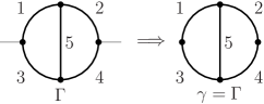
Figure 1: The diagram is composed of hard lines only; therefore, the naive expansion can be used.

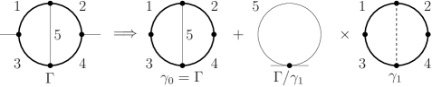
Figure 2: The diagram has one light line, as a consequence, non-trivial subgraph $\gamma_{1}$ is also needed.

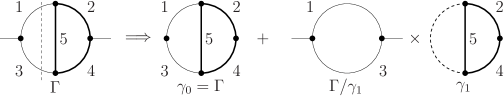
Figure 3: The diagram has one cut composed of two light lines, so non-trivial subgraph $\gamma_{1}$ has to be taken into account.

3 The running mass of the $t$-quark and its anomalous dimension

As was mentioned above running $\overline{\rm DR}$-mass of a quark is defined as renormalized quark mass in modified $\overline{\rm DR}$ renormalization scheme. In supersymmetric QCD we have the following relation between bare quark mass $m_{0}$ and its running $\overline{\rm DR}$-mass $m(\bar{\mu})$ at the scale $\bar{\mu}$:

$$m_{0}=m(\bar{\mu})\left\{1+\frac{\alpha_{s}}{4\pi}\frac{\delta Z_{m}^{(1)}}{\varepsilon}+\frac{\alpha_{s}^{2}}{(4\pi)^{2}}\left(\frac{\delta Z_{m}^{(2,1)}}{\varepsilon}+\frac{\delta Z_{m}^{(2,2)}}{\varepsilon^{2}}\right)\right\},$$ (11)

where $\alpha_{s}=g_{s}^{2}/(4\pi)$,

$$\delta Z_{m}^{(1)} = -2C_{F},$$ (12)

$$\delta Z_{m}^{(2,1)} = \phantom{-}6C_{F}-3C_{A}C_{F}+2C_{F}^{2},$$ (13)

$$\delta Z_{m}^{(2,2)} = -6C_{F}+3C_{A}C_{F}+2C_{F}^{2}$$ (14)

and $C_{F}=4/3,C_{A}=3$ are casimirs of $SU(3)$. Anomalous dimension of the quark mass $\gamma_{m}$ is defined as

$$\frac{d}{d\log{\bar{\mu}^{2}}}m(\bar{\mu})=\gamma_{m}m(\bar{\mu})$$ (15)

We consider two ways of obtaining quark mass anomalous dimension. As we know physical quantities do not depend on the scale parameter $\bar{\mu}$ so it is possible to find perturbative expansion of $\gamma_{m}$ in coupling constants of the theory by differentiation of pole mass expressed in terms of running parameters (4). Also it is possible to extract mass anomalous dimension from bare mass assuming that it is renormalization group-invariant. In [4] it was noticed that in non-supersymmetric QCD in modified $\overline{\rm DR}$ scheme suggested by the authors of that work, these two definitions do not produce the same result. In this paper we checked that in supersymmetric QCD two procedures mentioned above renders the same result in spite of the fact that we had used the same renormalization prescription as in [4]. The reason of such a coincidence turns to be in the fact that in supersymmetric QCD gauge coupling and so-called evanescent coupling of $\varepsilon$-scalars renormalize in the same way, so we can set them equal to each other at any scale $\bar{\mu}$.

The final result for anomalous dimension of the quark mass in supersymmetric QCD in $\overline{\rm DR}$ looks like

$$\gamma_{m}=-2C_{F}\frac{\alpha_{s}}{4\pi}+\left(12C_{F}-6C_{F}C_{A}+4C_{F}^{2}\right)\frac{\alpha_{s}^{2}}{(4\pi)^{2}}$$ (16)

In a general theory with spontaneous gauge symmetry breaking Yukawa beta-functions do not coincide with anomalous dimension of corresponding fermion mass, see e.g. [12]. However, since the tree-level MSSM Higgs potential does not depend on strong coupling constant $\alpha_{s}$, and no loop corrections give contributions proportional to $\alpha_{s}$ only (intuitively: the vacuum is colorless), the $\alpha_{s}^{n}$ coefficients in the perturbative expansion of (16) should be identical to the corresponding terms of top quark Yukawa coupling beta-function. Comparing (16) with two-loop MSSM top quark Yukawa coupling beta-function [13, 14], one can see that $\alpha_{s}^{2}$ term of that beta-function indeed coincides with the corresponding term of the anomalous dimension (16). This gives an additional confirmation of the correctness of our result.

4 Numerical results

The analytical result of our calculation is complicated due to the presence of a large number of masses, and no phenomenologically acceptable limit seems to exist. Therefore, we present here the numerical analysis of our results.

Figure 4: Relative value of second-order term of large mass expansion $\sigma_{2}^{\mathrm{rel}}$ (see (17)) as a function of $m_{1/2}$.

First, let us discuss the relative value of second order terms of large mass expansion, i.e.

$$\sigma_{2}^{\mathrm{rel}}\equiv\left|\frac{\sigma_{2}^{(1)}(M_{Z})+\sigma_{2}^{(2)}(M_{Z})}{\sigma_{2}^{(-1)}(M_{Z})+\sigma_{2}^{(0)}(M_{Z})}\right|.$$ (17)

We investigated this quantity in the following regions of the CMSSM parameter space

$$600\;{\rm GeV}\leq m_{0}\leq 1000\;{\rm GeV}$$

$$200\;{\rm GeV}\leq m_{1/2}\leq 1000\;{\rm GeV}$$

for $a_{0}=0,\;0.4m_{0},\;-0.4m_{0}$ and $\tan\beta=33,\;50$. We only consider $\mu>0$ and large values of $\tan\beta$, since small $\tan\beta$ and negative $\mu$ seem to be excluded by experimental data [15]. We found that $\sigma_{2}^{\mathrm{rel}}\lesssim 10^{-3}$ in these regions. Typical behaviour of $\sigma_{2}^{\mathrm{rel}}$ is shown in Fig. 4. Thus, contribution of second order large mass expansion terms to the relation between the pole and running masses (7) is negligible.

Numerical values of running SUSY parameters at the $M_{Z}$ scale have been calculated as a function of CMSSM parameters with heavily modified version of SOFTSUSY [16] in the framework of the mSUGRA supersymmetry breaking scenario.

Figure 5: Two-loop ($\alpha_{s}^{2}$) and one-loop ($\alpha_{s}$) SQCD contributions to $\Delta m_{t}(M_{Z})/m_{t}(M_{Z})$. Solid lines correspond to SQCD corrections, dashed line correspond to “pupe QCD” ones.

In the original SOFTSUSY code (as of version 1.9) two-loop SQCD contribution to the relation (7) is neglected, while two-loop QCD contribution to that relation is taken into account. This approximation is not applicable in the region of CMSSM parameters we considered. Figure 5 demonstrates this. Fig. 5 shows $m_{1/2}$- and $m_{0}$-dependence of the $\mathcal{O}(\alpha_{s}^{2})$ supersymmetric QCD corrections to (7) (here and in what follows all SQCD corrections include contributions from “pure QCD” diagrams). For comparison we plotted 1-loop SQCD contribution and 2-loop QCD contribution. One can see that

1. two-loop SQCD correction is about of 30% of the one-loop one,

2. two-loop SQCD contribution is of the same order of magnitude as one-loop QCD correction,

3. two-loop QCD contribution is about of 20% of total two-loop SQCD correction.

Thus, two-loop SQCD correction to the relation between the pole and running masses of the $t$-quark is not negligible and should be taken into account in phenomenological analysis of MSSM.

Figure 6: Masses of heavy Higgs bosons and chargino as a functions of $m_{1/2}$. Dashed lines correspond to the output of the original SOFTSUSY code (two-loop SQCD contribution to $\Delta m_{t}(M_{Z})/m_{t}(M_{Z})$ is neglected), solid lines correspond to the same code with above mentioned SQCD corrections. Gray regions represent discrepancies between the values of masses predicted by different programs for calculation of MSSM mass spectrum [19]. Here $\tan\beta=50,\;A_{0}=0,\;m_{0}=1000\;{\rm GeV}$

Taking into account this correction yields sizable change (more than 10%) of predicted masses of heavy Higgs bosons and chargino (see Fig. 6). This fact represents strong dependence of $\mu$ and $M_{A}$ on the heavy quark Yukawa couplings in certain regions of parameter space [18]. This dependence leads to relatively large discrepancies [18, 19] between the values of predicted masses given by different software for calculation of MSSM mass spectrum [16, 17]. It should be noted that change due to two-loop SQCD correction to the relation (7) exceeds these discrepancies.

Figure 7: Change of predicted mass of the lightest Higgs boson and the lightest neutralino mass due to two-loop SQCD contribution to $\Delta m_{t}(M_{Z})/m_{t}(M_{Z})$ as a function of $m_{1/2}$. Here $m_{0}=1000\,{\rm GeV},\,\tan\beta=50,\,A_{0}=0$.

However, masses of squarks, gluino, and relatively light particles (lightest neutralino, lightest Higgs boson) do not obtain any significant changes due to above mentioned two-loop SQCD contribution, see Fig. 7.

5 Conclusion

In this paper, we presented the result of calculation of the two-loop corrections to the relation between pole and running masses of the $t$-quark in the supersymmetric QCD. We provided a numerical analysis of the value of these corrections in different regions of the CMSSM parameter space. Our analysis showed that calculated second-order terms of large mass expansion $\mathcal{O}(m_{t}^{2}/M_{hard}^{2})$ give negligible contribution to this relation, so zero-order result given in [1] provides reliable approximation for phenomenological studies of the MSSM. Analysis given in [18] demonstrates that there exists two regions of the MSSM parameter space where accurate predictions based on computer codes [16, 17] are difficult: the large $\tan\beta$ and focus-point regimes. These two regions require a more precise determination of the heavy quark Yukawa couplings, or equivalently a more precise determination of running quark masses. We showed that two-loop supersymmetric QCD corrections give sizable contribution to (10) and has to be included in computer codes used to calculate MSSM spectra [16, 17].

As a by-product of our calculation, we also obtained two-loop anomalous dimension of the running quark $\overline{\rm DR}$-mass in the supersymmetric QCD.

6 Acknowledgements

The authors would like to thank M. Yu. Kalmykov for fruitful discussions and multiple comments. Financial support from RFBR grant # 05-02-17603, grant of the Ministry of Industry, Science and Technologies of the Russian Federation # 2339.2003.02 is kindly acknowledged.

References

- [1] A. Bednyakov, A. Onishchenko, V. Velizhanin and O. Veretin, Eur. Phys. J. C 29 (2003) 87 [arXiv:hep-ph/0210258].
-
[2]
V. A. Smirnov,
“Applied asymptotic expansions in momenta and masses,”
ISBN: 3540423346, Springer-Verlag (2001) (Springer tracts in modern physics, 177),
http://www.slac.stanford.edu/spires/find/hep/www?irn=4841620
A. N. Kuznetsov, F. V. Tkachov and V. V. Vlasov, arXiv:hep-th/9612037.
A. N. Kuznetsov and F. V. Tkachov, arXiv:hep-th/9612038.
F. V. Tkachov, Int. J. Mod. Phys. A 8, 2047 (1993) [arXiv:hep-ph/9612284]. - [3] A. Bednyakov and A. Sheplyakov, Phys. Lett. B 604, 91 (2004) [arXiv:hep-ph/0410128].
- [4] L. V. Avdeev and M. Y. Kalmykov, Nucl. Phys. B 502, 419 (1997) [arXiv:hep-ph/9701308].
- [5] F. A. Berends, A. I. Davydychev and V. A. Smirnov, Nucl. Phys. B 478, 59 (1996) [arXiv:hep-ph/9602396].
- [6] T. Hahn and C. Schappacher, Comput. Phys. Commun. 143, 54 (2002) [arXiv:hep-ph/0105349].
- [7] A. Sheplyakov, “prop2exp, a C++ library for asymptotic expansion of 2-loop propagator type integrals,” unpublished. The source code can be obtained form http://theor.jinr.ru/~varg/dist
- [8] C. Bauer, A. Frink and R. Kreckel, arXiv:cs.sc/0004015.
- [9] A. Sheplyakov, “bubblesII, a C++ library for analytical and numerical evaluation of 2-loop vacuum integrals,” unpublished. The source code can be obtained form http://theor.jinr.ru/~varg/dist
- [10] A. I. Davydychev and J. B. Tausk, Nucl. Phys. B 397, 123 (1993).
-
[11]
F. V. Tkachov,
Phys. Lett. B 100, 65 (1981).
K. G. Chetyrkin and F. V. Tkachov, Nucl. Phys. B 192, 159 (1981). - [12] F. Jegerlehner and M. Y. Kalmykov, Acta Phys. Polon. B 34, 5335 (2003) [arXiv:hep-ph/0310361].
- [13] D. J. Castano, E. J. Piard and P. Ramond, Phys. Rev. D 49, 4882 (1994) [arXiv:hep-ph/9308335].
- [14] S. P. Martin and M. T. Vaugh:, Phys. Rev. D 50, 2282 (1994) [arXiv:hep-ph/9311340].
-
[15]
W. de Boer, M. Huber, C. Sander and D. I. Kazakov,
Phys. Lett. B 515, 283 (2001).
H. Baer, C. Balazs, A. Belyaev, T. Krupovnickas and X. Tata, JHEP 0306, 054 (2003) [arXiv:hep-ph/0304303].
W. de Boer and C. Sander, Phys. Lett. B 585, 276 (2004) [arXiv:hep-ph/0307049].
J. R. Ellis, K. A. Olive, Y. Santoso and V. C. Spanos, arXiv:hep-ph/0408118. - [16] B. C. Allanach, Comput. Phys. Commun. 143, 305 (2002) [arXiv:hep-ph/0104145].
-
[17]
A. Djouadi, J. L. Kneur and G. Moultaka,
arXiv:hep-ph/0211331.
W. Porod, Comput. Phys. Commun. 153, 275 (2003) [arXiv:hep-ph/0301101].
F. E. Paige, S. D. Protopescu, H. Baer and X. Tata, arXiv:hep-ph/0312045. - [18] B. C. Allanach, S. Kraml and W. Porod, JHEP 0303, 016 (2003) [arXiv:hep-ph/0302102].
- [19] G. Belanger, S. Kraml and A. Pukhov, arXiv:hep-ph/0502079.