Trapping Black Hole Remnants
Abstract
Large extra dimensions lower the Planck scale to values soon accessible. The production of TeV mass black holes at the LHC is one of the most exciting predictions. However, the final phases of the black hole’s evaporation are still unknown and there are strong indications that a black hole remnant can be left. Since a certain fraction of such objects would be electrically charged, we argue that they can be trapped. In this paper, we examine the occurrence of such charged black hole remnants.
These trapped remnants are of high interest, as they could be used to closely investigate the evaporation characteristics. Due to the absence of background from the collision region and the controlled initial state, the signal would be very clear. This would allow to extract information about the late stages of the evaporation process with high precision.
I Extra Dimensions
Models with large extra dimensions (LXDs) are motivated by string theory [1] and provide us with an effective description of physics beyond the standard model (SM) in which observables can be computed and predictions can be made. Arkani-Hamed, Dimopoulos and Dvali [2] proposed a solution to the hierarchy problem by the introduction of additional compactified space-like dimensions in which only the gravitons can propagate. The SM particles are bound to our 4-dimensional sub-manifold, often called our 3-brane.
This yields an attractive and simple explanation of the hierarchy problem. Consider a particle of mass located in a space time with dimensions. The general solution of Poisson’s equation yields its potential as a function of the radial distance to the source
| (1) |
where a new fundamental mass-scale, , has been introduced.
The additional space-time dimensions are compactified on radii , which are small enough to have been unobserved so far. Then, at distances the potential Eq. (1) will turn into the common potential, but with a pre-factor given by the volume of the extra dimensions
| (2) |
In the limit of large distances, rediscovering the usual gravitational law yields the relation
| (3) |
It can be seen from this argument that the volume of the extra dimensions suppresses the fundamental scale and thus, can explain the huge value of the observed Planck mass TeV.
The radius of these extra dimensions, for TeV, can be estimated with Eq.(3) and typically lies in the range from mm to fm for from to , or the inverse radius lies in energy range eV to MeV, respectively.
LXDs predict a vast number of new effects at energies close to the new fundamental scale. Among the signatures are modifications of SM observables due to virtual graviton exchange, the production of real gravitons and TeV-scale black holes. For recent constraints from collider searches and astrophysics see e.g. [4].
II Black Holes in Extra Dimensions
Using the higher dimensional Schwarzschild-metric [5], it can be derived that the horizon radius of a black hole is substantially increased in the presence of LXDs, reflecting the fact that gravity at small distances becomes stronger. For a black hole of mass one finds
| (4) |
The horizon radius for a black hole with mass TeV is then fm, and thus for black holes which might possibly be produced at colliders or in ultra high energetic cosmic rays.
Black holes with masses in the range of the lowered Planck scale should be a subject of quantum gravity. Since there is yet no theory available to perform this analysis, the black holes are treated as semi classical objects. The gravitational field is classical, though the evaporation process is a quantum effect.
To compute the production details, the cross-section of the black holes can be approximated by the classical geometric cross-section
| (5) |
an expression which contains only the fundamental Planck scale as coupling constant. This cross section is a subject of ongoing research [7] but close investigations justify the use of the classical limit at least up to energies of [8]. It has further been shown that the naively expected classical result remains valid also in string theory [9].
A common approach to improve the naive picture of colliding point particles, is to treat the creation of the horizon as a collision of two shock fronts in an Aichelburg-Sexl geometry describing the fast moving particles [10, 11]. Due to the high velocity of the moving particles, space time before and after the shocks is almost flat and the geometry can be examined for the occurrence of trapped surfaces.
These semi classical considerations do also give rise to form factors which take into account that not the whole initial energy is captured behind the horizon. These factors have been calculated in [12], depend on the number of extra dimensions, and are of order one. They are included in our numerical evaluation. The scattering of the emitted particle on the gravitational potential is also taken into account in the graybody factors [13].
Setting TeV and one finds TeV pb. With this it is further found that these black holes will be produced at LHC. For the estimated luminosity of 100/fb more than black holes are expected per year [14]. The potential importance of the black hole production at colliders has been investigated in numerous publications, see e.g. [16, 17] and References therein.
Once produced, the black holes will undergo an evaporation process whose thermal properties carry information about the parameters and . An analysis of the evaporation will therefore offer the possibility to extract knowledge about the topology of our space time and the underlying theory.
The evaporation process can be categorised in three characteristic stages [15]: the balding phase, the evaporation phase and the Planck phase. It is generally assumed that in the last phase, the black hole will either completely decay in a few SM particles or a stable remnant will be left, which carries away the remaining energy. In the following we will focus on the case in which a remnant of approximately Planck mass is left.
For more details on the topic of TeV-scale black holes, the interested reader is referred to the reviews [19].
III Black Hole Remnants
The final fate of these evaporating black holes is closely connected to the information loss puzzle. The black hole emits thermal radiation, whose sole property is the temperature, regardless of the initial state of the collapsing matter. So, if the black hole completely decays into statistically distributed particles, unitarity can be violated. This happens when the initial state is a pure quantum state and then evolves into a mixed state [20].
When one tries to avoid the information loss problem two possibilities are left. The information is regained by some unknown mechanism or a stable black hole remnant is formed which keeps the information. Besides the fact that it is unclear in which way the information should escape the horizon [21] there are several other arguments for black hole remnants [22]:
-
The uncertainty relation: The Schwarzschild radius of a black hole with Planck mass is of the order of the Planck length. Since the Planck length is the wavelength corresponding to a particle of Planck mass, a problem arises when the mass of the black hole drops below Planck mass. Then one has trapped a mass inside a volume which is smaller than allowed by the uncertainty principle [23]. To avoid this problem, Zel’dovich has proposed that black holes with masses below Planck mass should be associated with stable elementary particles [24].
-
Corrections to the Lagrangian: The introduction of additional terms, which are quadratic in the curvature, yields a dropping of the evaporation temperature towards zero [25]. This holds also for extra dimensional scenarios [26] and is supported by calculations in the low energy limit of string theory [27].The production of TeV-scale black holes in the presence of Lovelock higher-curvature terms has been examined in [28] and it was found that these black holes can become thermodynamically stable since their evaporation takes an infinite amount of time.
-
Further reasons for the existence of remnants have been suggested: E.g. black holes with axionic charge [29], the modification of the Hawking temperature due to quantum hair [30] or magnetic monopoles [31]. Coupling of a dilaton field to gravity also yields remnants, with detailed features depending on the dimension of space-time [32].
Of course these remnants, which have also been termed Maximons, Friedmons, Cornucopions, Planckons or Informons, are not a miraculous remedy but bring some problems on their own, e.g. the necessity for an infinite number of states which allows the unbounded information content inherited from the initial state.
In [33], it has been shown that the black hole remnants give rise to distinct collider signatures. In the present work we will in particular examine the properties of charged remnants.
IV Charged Black Holes
The black hole produced in a proton-proton collision can carry an electric charge. The evaporation spectrum contains all particles of the SM and so, a certain fraction of the final black hole remnants will also carry net electric charge. In the following, these charged black hole remnants will be denoted and , and the neutral ones , respectively. Since the ’s undergo an electromagnetic interaction, their cross section is enhanced and they can be examined closely. This makes them extremely interesting candidates for the investigation of Planck scale physics.
The metric of a charged black hole in higher dimensions has been derived in [5]. This solution assumes the electric field to be spherical symmetric in all dimensions whereas in the scenario with LXDs the SM fields are confined to our brane. This has also been pointed out in Ref. [34].
The exact solution for this system in a spacetime with compacitfied extra dimensions is known only implicitely [6]. However, for our purposes, it will be sufficient to estimate the charge effects by taking into account that we expect the brane to have a width of about . Up to this width, also the gauge fields can penetrate the bulk which is essentially a scenario of embedding universal extra dimensions as a fat brane into the large extra dimensions. Note, that this does not modify the electromagnetic coupling constants as there is no hierarchy between the inverse width and the radius of the fat brane. Following the same arguments leading to the Newtonian potential (Eq.(1)), we see that the Coulomb potential receives a modification to
| (6) |
where is the fine structure constant and is the dimensionless charge in units of the unit charge . But this higher dimensional potential will already turn into the usual potential at a distance which means that the pre-factors cancel and does not collect any volume factors.
One can estimate the exact solution for the system by assuming it to be spherical symmetric up to the horizon radius. This yields
| (7) |
where is the potential containing the gravitational energy and the Coulomb energy of the source whose electric field is now also higher dimensional. The weak field limit of Einsteins field equations yields the Poisson equation
| (8) |
where is the surface of the -dimensional unit sphere
| (9) |
and the delta-function is already converted into spherical coordinates. Using the spherical symmetry and applying Gauss’ Law yields then
| (10) |
And so we find
| (11) |
The horizon is located at the zero of . In case there exists no (real) solution for , the metric is dominated by the contribution of the electromagnetic field and the singularity will be a naked one. The requirement of having a zero yields the constraint***Note, that these relations do only agree with the relations in [5] up to geometrical pre-factors. This is due to the fact that our additional dimensions are compactified and the higher dimensional coupling constants are fixed by Eq (3) and (6).
| (12) |
With few , and being close by , the left hand side is at least by a factor smaller than the right hand side. So, the charge contribution to the gravitational field, which is described by the second term of Eq.(11), will be negligible at the horizon location . For the typical collider produced black holes, the singularity will not be naked. For the same reason, modifications of the Hawking evaporation spectrum can be neglected in the charge range under investigation.
Let us briefly comment on the assumption that the electromagnetic field is spherical symmetric up to a brane width of . If the field is confined to a thinner brane, the charge contribution to the gravitational potential will obey a different functional behaviour. It will drop slower at large distances but therefore be less divergent at small distances. This means, if the above inequality is fulfilled it will still hold because the singularity is even better shielded.
Usually, the Hawking radiation for very small charged black holes necessarily leads to naked singularities which are hoped to be excluded by the (unproven) cosmic censorship hypothesis. The reason is that once the mass of a charged black hole becomes smaller than the mass of the lightest charged particle - i.e. the electron or positron, respectively - it could never get rid of its charge by radiating it off. Then, it would either end as a naked singularity or as a tiny remnant of mass about the electron mass. This case, however, can not occur in the here discussed setting as we assume the remnant mass to be close by and therefore much above the electron mass.
V Charged Black Hole Remnants
Black holes are typically formed from valence quarks as those carry the largest available momenta of the partonic system. So, the black holes formed in a proton-proton collision will have an average charge of . The black holes decay with an average multiplicity of into particles of the SM, most of which will be charged. The details of the multiplicity depend on the number of extra dimensions [33]. After the black holes have evaporated off enough energy to be stable at the remnant mass, some have accumulated a net electric charge. According to purely statistical considerations, the probability for being left with highly charged black hole remnants drops fast with deviation from the average. The largest fraction of the black holes should have charges or zero.
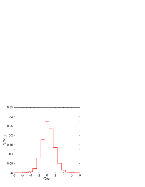
For a detailed analysis, we have estimated the fraction of charged black hole remnants with the PYTHIA event generator and the CHARYBDIS program [35, 36]. For our purposes, we turned off the final decay of the black hole and the charge minimization. Figure 1 shows the results for a simulation of proton-proton collisions at the LHC with an estimated center of mass energy of TeV.
We further assumed as an applicable model, worked out in [33], that the effective temperature of the black hole drops towards zero for a finite remnant mass . This mass of the remnant is a few and a parameter of the model. Even though the temperature-mass relation is not clear from the present status of theoretical examinations, such a drop of the temperature can be implemented into the simulation. However, the details of the modified temperature as well as the value of do not noticeably affect the here investigated charge distribution as it results from the very general statistical distribution of the charge of the emitted particles.
Therefore, independent of the underlying quantum gravitational assumption leading to the remnant formation, we find that about % of the remnants carry zero electric charge, whereas we have % of and % of .
The total number of produced black hole remnants depends on the total cross section for black holes [16, 17, 37, 38]. Ongoing investigations on the subject reveal a strong dependence on and a slight dependence on and suggest the production of black holes per year. Thus, following the above given results we predict the production of about single charged remnants per year.
These charged black hole remnants are of special importance. Once produced, the could be singled out in an experiment before they are neutralized in a detector. The characteristically small makes them easy to distinguish from particles of the SM. Their electromagnetic interaction further allows it to trap and keep them in an electromagnetic field.
For the specific scenario discussed here, the average momenta of the black hole remnants are of the order of TeV. We suggest to use a similar approach as used for the trapping of anti-protons at LEAR/TRAP [39]. This means, first the remnants are decelerated in a decelerator ring from some GeV/c down to 100 MeV/c. Then they have to be further slowed down by electric fields to a couple of keV. This is slow enough to allow for a capture of the remnants in a Penning trap with low temperature. Then positrons (or electrons) are loaded into the trap. The positrons/electrons cool down to the temperature of the Penning trap by the emission of cyclotron radiation. Unfortunately, the lower cyclotron frequency of the heavy (thus slow) remnants makes this cooling mechanism less efficient for black hole remnants. However, they can be cooled indirectly by Coulomb interaction with the positrons or electrons.

In the case of anti-protons, the above discussed method allowed the TRAP collaboration to store the anti-protons for many month. This time would be sufficient to collect a huge amount of black hole remnants for study, even if only a small percentage will have low enough energies for deceleration.
Another approach to collect black hole remnants might be to slow down the charged remnants by energy loss in matter - a similar approach was suggested by [40] to stop gluinos. The energy loss experienced by a charged particle when travelling through matter can be calculated using the Bethe-Bloch equation. ¿From the average momentum of the remnants, we conclude that 50% of the remnants will have velocities . I.e. these remnants can be decelerated in matter e.g. in an iron block of 8 cm (), 1.3 m () or 6.4 m () length. This method would allow to include even high momentum remnants into the trapping process.
Thus, these approaches indicates the possibility to accumulate separated and over a long period of time.
In a second stage, the s can be merged with the s which increases the horizon in the process . During this process, the charge of the forming black hole is neutralized and the mass is increased to . This will make a new evaporation possible which can then be analyzed in an environment clean of background from the proton-proton collision. In particular, the characteristics of the late stages of the decay can be observed closely.
After the merged black holes have shrunk again to remnant mass, most of them will be neutral and escape the experimentally accessible region due to their small cross section.
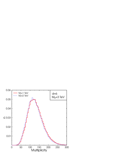
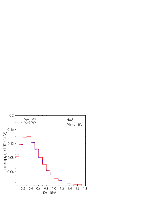
Figure 2 to 5 show results from a simulation of such reactions for a sample of events of with CHARYBDIS modified to incorporate the remnant production according to [33]. Here, we have assumed that the black holes have been slowed down enough to make the initial momentum negligible. The total energy of the collision is then . Figure 2 and 3 show the total multiplicity of the events after fragmentation, Figures 4 and 5 show the - spectra for ’s as an example . The spectra are free from low energetic debris present in collisions arising from the presence of spectators.
Even though the parameter of the model might be difficult to extract (the dependence on and would require initial states of varying masses) a measurement of such spectrum would be a very important input to examine the signatures from the collision at the LHC. In such a way, the remnants would allow to extract the properties of the black hole’s decay and remove theoretical uncertainties by allowing to quantify them directly from experimental measurements. This would substantially increase the precision by which the parameters of the underlying extra-dimensional model can be determined.

VI Conclusion
In the scenario of large extra dimensions, the formation of black hole remnants in high energy collisions is possible. We have computed the fraction of charged black hole remnants. With use of the PYTHIA event generator we found that about 23.5% of the remnants carry charge and 17.7% carry charge . Due to their electromagnetic interaction, we have argued that the black hole remnants can be trapped and then could be used to examine the evaporation characteristics. In this case, the absence of background from the collision region and the controlled initial state would allow to obtain very clean signals. This would make it possible to extract information about the late stages of the evaporation process of black holes with unprecedented precision.
Acknowledgements
We thank Horst Stöcker for helpful discussions. This work was supported by NSF PHY/0301998 and DFG. SH wants to thank the FIAS for kind hospitality.
References
REFERENCES
- [1] I. Antoniadis, Phys. Lett. B 246, 377 (1990); I. Antoniadis and M. Quiros, Phys. Lett. B 392, 61 (1997); K. R. Dienes, E. Dudas and T. Gherghetta, Nucl. Phys. B 537, 47 (1999).
- [2] N. Arkani-Hamed, S. Dimopoulos and G. R. Dvali, Phys. Lett. B 429, 263 (1998); I. Antoniadis, N. Arkani-Hamed, S. Dimopoulos and G. R. Dvali, Phys. Lett. B 436, 257 (1998); N. Arkani-Hamed, S. Dimopoulos and G. R. Dvali, Phys. Rev. D 59, 086004 (1999).
- [3] K. R. Dienes, E. Dudas and T. Gherghetta, Phys. Lett. B 436, 55 (1998).
- [4] K. Cheung, [arXiv:hep-ph/0409028]; G. Landsberg, [arXiv:hep-ex/0412028].
- [5] R. C. Myers and M. J. Perry Ann. Phys. 172, 304-347 (1986).
- [6] S. D. Majumdar, Phys. Rev. 72 (1947) 390; A. Papapetrou, Proc. R. Irish Acad. A51, (1947) 191; R. C. Myers, Phys. Rev. D 35 (1987) 455. D. Korotkin and H. Nicolai, [arXiv:gr-qc/9403029]; D. Korotkin and H. Nicolai, Nucl. Phys. B 429 (1994) 229; A. V. Frolov and V. P. Frolov, Phys. Rev. D 67 (2003) 124025; T. Harmark and N. A. Obers, JHEP 0205 (2002) 032; T. Harmark and N. A. Obers, Nucl. Phys. B 684 (2004) 183; D. Gorbonos and B. Kol, JHEP 0406 (2004) 053; D. Gorbonos and B. Kol, [arXiv:hep-th/0505009]; M. Karlovini and R. von Unge, [arXiv:gr-qc/0506073].
- [7] M. B. Voloshin, Phys. Lett. B 518, 137 (2001); Phys. Lett. B 524, 376 (2002); S. B. Giddings, in Proc. of the APS/DPF/DPB Summer Study on the Future of Particle Physics (Snowmass 2001) ed. N. Graf, eConf C010630, P328 (2001).
- [8] S. N. Solodukhin, Phys. Lett. B 533, 153 (2002); A. Jevicki and J. Thaler, Phys. Rev. D 66, 024041 (2002); T. G. Rizzo, in Proc. of the APS/DPF/DPB Summer Study on the Future of Particle Physics (Snowmass 2001) ed. N. Graf, eConf C010630, P339 (2001); D. M. Eardley and S. B. Giddings, Phys. Rev. D 66, 044011 (2002).
- [9] G. T. Horowitz and J. Polchinski, Phys. Rev. D 66 103512 (2002).
- [10] V. S. Rychkov, Phys. Rev. D 70, 044003 (2004); K. Kang and H. Nastase, [arXiv:hep-th/0409099].
- [11] I. Ya. Yref’eva, Part.Nucl. 31, 169-180 (2000). S. B. Giddings and V. S. Rychkov, Phys. Rev. D 70, 104026 (2004); V. S. Rychkov, [arXiv:hep-th/0410041]; T. Banks and W. Fischler, [arXiv:hep-th/9906038]. O. V. Kancheli, [arXiv:hep-ph/0208021].
- [12] H. Yoshino and Y. Nambu, Phys. Rev. D 67, 024009 (2003).
- [13] S. N. Solodukhin, Phys. Lett. B 533 153-161 (2002); D. Ida, K. y. Oda and S. C. Park, Phys. Rev. D 67, 064025 (2003).
- [14] S. Dimopoulos and G. Landsberg Phys. Rev. Lett. 87, 161602 (2001); P.C. Argyres, S. Dimopoulos, and J. March-Russell, Phys. Lett. B441, 96 (1998).
- [15] S. B. Giddings and S. Thomas, Phys. Rev. D 65 056010 (2002).
- [16] L. Anchordoqui and H. Goldberg, Phys. Rev. D 67, 064010 (2003); K. Cheung, Phys. Rev. D 66, 036007 (2002); K. m. Cheung, Phys. Rev. Lett. 88, 221602 (2002); S. C. Park and H. S. Song, J. Korean Phys. Soc. 43, 30 (2003); S. Hossenfelder, S. Hofmann, M. Bleicher and H. Stocker, Phys. Rev. D 66, 101502 (2002); M. Bleicher, S. Hofmann, S. Hossenfelder and H. Stocker, Phys. Lett. B 548, 73 (2002); M. Cavaglia, S. Das and R. Maartens, Class. Quant. Grav. 20, L205 (2003); M. Cavaglia and S. Das, Class. Quant. Grav. 21, 4511 (2004); S. Hossenfelder, Phys. Lett. B 598, 92 (2004); I. Mocioiu, Y. Nara and I. Sarcevic, Phys. Lett. B 557, 87 (2003); A. Ringwald, Fortsch. Phys. 51, 830 (2003).
- [17] A. Chamblin and G. C. Nayak, Phys. Rev. D 66, 091901 (2002).
- [18] R. Emparan, G. T. Horowitz and R. C. Myers Phys. Rev. Lett. 85, 499 (2000).
- [19] P. Kanti, Int. J. Mod. Phys. A 19 (2004) 4899. G. Landsberg, [arXiv:hep-ph/0211043]; M. Cavaglia, Int. J. Mod. Phys. A 18, 1843 (2003); S. Hossenfelder, [arXiv:hep-ph/0412265].
- [20] S. Hawking, Commun. Math. Phys. 87,395 (1982); J. Preskill, [arXiv:hep-th/9209058]; I. D. Novikov and V. P. Frolov, ”Black Hole Physics”, Kluver Academic Publishers (1998).
- [21] D. N. Page, Phys. Rev. Lett. 44, 301 (1980); G. t’Hooft, Nucl. Phys. B 256 727 (1985); A. Mikovic, Phys. Lett. 304 B, 70 (1992); E. Verlinde and H. Verlinde, Nucl. Phys. B 406, 43 (1993); L. Susskind, L. Thorlacius and J. Uglum, Phys. Rev. D 48, 3743 (1993); D. N. Page, Phys. Rev. Lett. 71 3743 (1993).
- [22] Y. Aharonov, A. Casher and S. Nussinov, Phys. Lett. 191 B, 51 (1987); T. Banks, A. Dabholkar, M. R. Douglas and M. O’Loughlin, Phys. Rev. D 45 3607 (1992); T. Banks and M. O’Loughlin, Phys. Rev. D 47, 540 (1993); T. Banks, M. O’Loughlin and A. Strominger, Phys. Rev. D 47, 4476 (1993); S. B. Giddings, Phys. Rev. D 49, 947 (1994); M. D. Maia, [arXiv:gr-qc/0505119]; V. Husain and O. Winkler, [arXiv:gr-qc/0505153].
- [23] M. A. Markov, in: ”Proc. 2nd Seminar in Quantum Gravity”, edited by M. A. Markov and P. C. West, Plenum, New York (1984).
- [24] Y. B. Zel’dovich, in: ”Proc. 2nd Seminar in Quantum Gravity”, edited by M. A. Markov and P. C. West, Plenum, New York (1984).
- [25] J. D. Barrow, E. J. Copeland and A. R. Liddle, Phys. Rev. D 46, 645 (1992); B. Whitt, Phys. Rev. D 38, 3000 (1988).
- [26] R. C. Myers and J. Z. Simon, Phys. Rev. D 38, 2434 (1988).
- [27] C. G. Callan, R. C. Myers and M. J. Perry, Nucl. Phys. B 311, 673 (1988); S. Alexeyev, A. Barrau, G. Boudoul, O. Khovanskaya and M. Sazhin, Class. Quant. Grav. 19, 4431-4444 (2002).
- [28] T. G. Rizzo, [arXiv:hep-ph/0503163]; T. G. Rizzo, [arXiv:hep-ph/0504118].
- [29] M. J. Bowick, S. B. Giddings, J. A. Harvey, G. T. Horowitz and A. Strominger, Phys. Rev. Lett. 61 2823 (1988).
- [30] S. Coleman, J. Preskill and F. Wilczek, Mod. Phys. Lett. A6 1631 (1991).
- [31] K-Y. Lee, E. D. Nair and E. Weinberg, Phys. Rev. Lett. 68 1100 (1992).
- [32] G. W. Gibbons and K. Maeda, Nucl. Phys. B 298 741 (1988); T. Torii and K. Maeda, Phys. Rev. D 48 1643 (1993).
- [33] B. Koch, M. Bleicher and S. Hossenfelder, ”Black Hole Remnants at the LHC”, [hep-ph/0507138].
- [34] R. Casadio and B. Harms, Int. J. Mod. Phys. A 17, 4635 (2002);
- [35] T. Sjostrand, L. Lonnblad and S. Mrenna, [arXiv:hep-ph/0108264].
-
[36]
C. M. Harris, P. Richardson and B. R. Webber,
JHEP 0308, 033 (2003)
[arXiv:hep-ph/0307305].
URL for downloading: www.ippp.dur.ac.uk/ montecarlo/leshouches/generators/charybdis/ - [37] J. Tanaka, T. Yamamura, S. Asai and J. Kanzaki, [arXiv:hep-ph/0411095].
- [38] C. M. Harris, M. J. Palmer, M. A. Parker, P. Richardson, A. Sabetfakhri and B. R. Webber, [arXiv:hep-ph/0411022].
- [39] G. Gabrielse et al., Phys. Rev. Lett. 63 (1989) 1360.
- [40] A. Arvanitaki, S. Dimopoulos, A. Pierce, S. Rajendran and J. Wacker, arXiv:hep-ph/0506242.