Black Hole Remnants at the LHC

Abstract:

Within the scenario of large extra dimensions, the Planck scale is lowered to values soon accessible. Among the predicted effects, the production of TeV mass black holes at the LHC is one of the most exciting possibilities. Though the final phases of the black hole’s evaporation are still unknown, the formation of a black hole remnant is a theoretically well motivated expectation. We analyze the observables emerging from a black hole evaporation with a remnant instead of a final decay. We show that the formation of a black hole remnant yields a signature which differs substantially from a final decay. We find the total transverse momentum of the black hole event to be significantly dominated by the presence of a remnant mass providing a strong experimental signature for black hole remnant formation.

1 Introduction

High energetic particle collisions will eventually lead to strong gravitational interactions and result in the formation of a black hole’s horizon. In the presence of large additional compactified dimensions [1], it could be possible that the threshold for black hole production lies within the accessible range for future experiments (e.g. LHC, CLIC). In the context of models with such large extra dimensions, black hole production is predicted to drastically change high energy physics already at the LHC. These effective models with extra dimensions are string-inspired [2, 3, 4] extensions to the Standard Model in the overlap region between ’top-down’ and ’bottom-up’ approaches.

The possible production of TeV-scale black holes at the LHC is surely one of the most exciting predictions of physics beyond the Standard Model and has received a great amount of interest during the last years [5, 6, 7, 8, 9, 10, 11, 12, 13, 14, 15, 16, 17, 18, 19, 20]. For reviews on the subject the interested reader is referred to [21].

Due to their Hawking-radiation [22], these small black holes will have a temperature of some $100$ GeV and will decay quickly into $\sim 10-25$ thermally distributed particles of the Standard Model (before fragmentation of the emitted partons). This yields a signature unlike all other new predicted effects. The black hole’s evaporation process connects quantum gravity with quantum field theory and particle physics, and is a promising way towards the understanding of Planck scale physics.

Thus, black holes are a fascinating field of research which features an interplay between General Relativity, thermodynamics, quantum field theory, and particle physics. The investigation of black holes would allow to test Planck scale effects and the onset of quantum gravity. Therefore, the understanding of the black holes properties is a key knowledge to the phenomenology of physics beyond the Standard Model.

Recently, the production of black holes has been incorporated into detailed numerical simulations for black hole production and decay in ultra-high energetic hadron-hadron interactions [23, 24, 25].

So far the numerical simulation has assumed that the black hole decays in its final phase completely into some few particles of the Standard Model. However, from the theoretical point of view, there are strong indications that the black hole does not evaporate completely, but leaves a stable black hole remnant. In this work, we will include this possibility into the numerical simulation and examine the consequences for the observables of the black hole event. These investigations might allow to reconstruct initial parameters of the model from observed data and can shed light onto these important questions.

The aim of this investigation is not to derive the formation of a remnant from a theory of modified gravity but to incorporate the assumption of such a remnant into the possible signatures black hole events in high energetic particle interactions.

This paper is organized as follows: the next section briefly reviews basic facts about black holes in extra dimensions. Section 3 discusses the issue of black hole remnants and introduces a useful parametrization for the thermodynamical treatment. In section 4, we discuss the results of the numerical simulation. We conclude in section 5.

Throughout this paper we adopt the convention $\hbar=c=k_{B}=1$.

2 Black Holes in Extra Dimensions

Arkani-Hamed, Dimopoulos and Dvali [1] proposed a solution to the hierarchy problem by the introduction of $d$ additional compactified space-like dimensions in which only gravitons can propagate. The Standard Model (SM) particles are bound to our 4-dimensional sub-manifold, called our 3-brane.

Gauss’ law then relates the fundamental mass scale of the extended theory, $M_{\rm f}$, to the apparent Planck scale, $m_{\rm p}\sim 10^{16}$ TeV, by the volume of the extra dimensions. In the case of toroidal compactification on radii of equal size this yields

$$m_{\rm p}^{2}=M_{\rm f}^{d+2}R^{d}\quad.$$ (1)

Thus, for large radii, the Planck scale can be lowered to a new fundamental scale, $M_{\rm f}$ which can lie close by the electroweak scale.

The radius $R$ of the extra dimensions is then in the range mm to $10^{3}$ fm for $d$ from $2$ to $7$, or the inverse radius $1/R$ lies in energy range eV to MeV, resp. Since this radii are large compared to the Planck scale, this setting is called a scenario with large extra dimensions (LXDs). For recent constraints on the parameter of the model see e.g. [26].

Using the higher dimensional Schwarzschild-metric [27], it can be derived that the horizon radius $R_{H}$ of a black hole is substantially increased in the presence of LXDs [6], reflecting the fact that gravity at small distances becomes stronger. For a black hole of mass $M$ one finds

$$R^{d+1}_{H}=\frac{1}{d+1}\frac{1}{M_{\rm f}^{d+1}}\frac{M}{M_{\rm f}}\quad.$$ (2)

The horizon radius for a black hole with mass $\approx$ TeV is then $\approx 10^{-3}$ fm, and thus $R_{H}\ll R$ for black holes which can possibly be produced at colliders or in ultra high energetic cosmic rays. Also in higher dimensions the entropy, $S$, of the black hole is proportional to its horizon surface which is given by

$${\cal{A}}_{(d+3)} = \Omega_{(d+3)}R_{H}^{d+2}$$ (3)

where $\Omega_{(d+3)}$ is the surface of the $d+3$-dimensional unit sphere

$$\Omega_{(d+3)}=\frac{2\pi^{\frac{d+3}{2}}}{\Gamma({\frac{d+3}{2}})}\quad.$$ (4)

Black holes with masses in the range of the lowered Planck scale should be a subject of quantum gravity. Since there is yet no theory available to perform these calculations, the black holes are treated as semi classical objects which form intermediate meta-stable states. Thus, the black holes are produced and decay according to the semi classical formalism of black hole physics.

To compute the production probability, the cross-section of the black holes can be approximated by the classical geometric cross-section [8, 9]

$$\sigma(M)\approx\pi R_{H}^{2}~{}\Theta(M-M_{{\rm min}})\quad,$$ (5)

an expression which contains only the fundamental Planck scale as coupling constant. $M_{\rm min}$ is the threshold above which the production can occur and expected to be a few $\times M_{\rm f}$. As has been shown recently [28], such a threshold arises naturally in certain types of higher order curvature gravity.

The semi classical black hole cross section [6, 8, 9] has been under debate [11], but further investigations justify the use of the classical limit at least up to energies of $\sim 10M_{\rm f}$ [12, 13, 14]. It has further been shown that the naively expected classical result remains valid also in string-theory [16]. However, this interesting topic is still a matter of ongoing research, see e.g. the very recent contributions in Refs. [19].

A common approach to improve the naive picture of colliding point particles, is to treat the creation of the horizon as a collision of two shock fronts in an Aichelburg-Sexl geometry describing the fast moving particles [15]. Due to the high velocity of the moving particles, space time before and after the shocks is almost flat and the geometry can be examined for the occurrence of trapped surfaces.

These semi classical considerations do also give rise to form factors which take into account that not the whole initial energy is captured behind the horizon. These factors have been calculated in [17] and depend on the number of extra dimensions, however their numerical values are of order one. Setting $M_{\rm f}\sim 1$TeV and $d=2$ one finds $\sigma\sim 1$ TeV${}^{-2}\sim 400$ pb. With this cross section it is further found that these black holes will be produced at the LHC in huge numbers on the order of $\sim 10^{9}$ per year [8].

Once produced, the black holes will undergo an evaporation process whose thermal properties carry information about the parameters $M_{\rm f}$ and $d$. An analysis of the evaporation will therefore offer the possibility to extract knowledge about the topology of our space time and the underlying theory.

The evaporation process can be categorized in three characteristic stages [9]:

1. Balding phase: In this phase the black hole radiates away the multi-pole moments it has inherited from the initial configuration, and settles down in a hairless state. During this stage, a certain fraction of the initial mass will be lost in gravitational radiation.

2. Evaporation phase: The evaporation phase starts with a spin down phase in which the Hawking radiation [22] carries away the angular momentum, after which it proceeds with the emission of thermally distributed quanta until the black hole reaches Planck mass. The radiation spectrum contains all Standard Model particles, which are emitted on our brane, as well as gravitons, which are also emitted into the extra dimensions. It is expected that most of the initial energy is emitted during this phase in Standard Model particles [7].

3. Planck phase: Once the black hole has reached a mass close to the Planck mass, it falls into the regime of quantum gravity and predictions become increasingly difficult. It is generally assumed that the black hole will either completely decay in some last few Standard Model particles or a stable remnant will be left, which carries away the remaining energy.

The evaporation phase is expected to be the most important phase for high energy collisions. The characteristics of the black hole’s evaporation in this phase can be computed using the laws of black hole thermodynamics and are obtained by first solving the field equations for the metric of the black hole, then deriving the surface gravity, $\kappa$, from which the temperature of the black hole follows via

$$T=\frac{\kappa}{2\pi}\quad.$$ (6)

By identifying the total energy of the system with the mass of the black hole one then finds the entropy $S$ by integrating the thermodynamical identity

$$\frac{\partial S}{\partial M}=\frac{1}{T}\quad,$$ (7)

which fixes the constant factor relating the entropy to the horizon surface. A possible additive constant is generally chosen such that the entropy is zero for vanishing horizon surface. In contrast to classical thermodynamical objects, this does not necessarily imply that the entropy vanishes at zero temperature, see e.g. [29].

By now, several experimental groups include black holes into their search for physics beyond the Standard Model. For detailed studies of the experimental signatures, PYTHIA 6.2 [30] has been coupled to CHARYBDIS [23] creating an event generator allowing for the simulation of black hole events and data reconstruction from the decay products. Previous analysis within this framework are summarized in Refs. [24, 25]. Ideally, the energy distribution of the decay products allows a determination of the temperature (by fitting the energy spectrum to the predicted shape) as well as of the total mass of the object (by summing up all energies). This then allows to reconstruct the scale $M_{\rm f}$ and the number of extra dimensions.

These analysis however, have so far omitted the possibility of a stable black hole remnant but assume instead a final decay into some few particles, whose number is treated as a free parameter ranging from $2-5$.

In the following we will examine the possibility that a stable black hole remnant of about Planck mass is left with use of the PYTHIA 6.2/CHARYBDIS event generator package.

3 Black Hole Remnants

The final fate of black holes is an unresolved subject of ongoing research. The last stages of the evaporation process are closely connected to the information loss puzzle. The black hole emits thermal radiation, whose sole property is the temperature, regardless of the initial state of the collapsing matter. So, if a black hole completely decays into statistically distributed particles, unitarity can be violated. This happens when the initial state is a pure quantum state and then evolves into a mixed state [31, 32, 33].

When one tries to avoid the information loss problem two possibilities are left. The information is regained by some unknown mechanism or a stable black hole remnant is formed which keeps the information. Besides the fact that it is unclear in which way the information should escape the horizon [34] there are several other arguments for black hole remnants [35]:

• The uncertainty relation: The Schwarzschild radius of a black hole with Planck mass is of the order of the Planck length. Since the Planck length is the wavelength corresponding to a particle of Planck mass, a problem arises when the mass of the black hole drops below Planck mass. Then one has trapped a mass inside a volume which is smaller than allowed by the uncertainty principle [36]. To avoid this problem, Zel’dovich has proposed that black holes with masses below Planck mass should be associated with stable elementary particles [37]. Also, the occurrence of black hole remnants within the framework of a generalized uncertainty principle has been investigated in [38, 39].

• Corrections to the Lagrangian: The introduction of additional terms, which are quadratic in the curvature, yields a decrease of the evaporation temperature towards zero [40, 41]. This holds also for extra dimensional scenarios [42] and is supported by calculations in the low energy limit of string theory [43, 44]. The production of TeV-scale black holes in the presence of Lovelock higher-curvature terms has been examined in [28] and it was found that these black holes can become thermodynamically stable since their evaporation takes an infinite amount of time.

• Further reasons for the existence of remnants have been suggested to be black holes with axionic charge [45], the modification of the Hawking temperature due to quantum hair [46] or magnetic monopoles [47]. Coupling of a dilaton field to gravity also yields remnants, with detailed features depending on the dimension of space-time [48, 49].

• One might also see the arising necessity for remnant formation by applying the geometrical analogy to the black hole and quantize the radiation into wavelengths that fit on the surface, i.e. the horizon [50]. The smaller the size of the black hole, the smaller the largest possible wavelength and the larger the smallest possible energy quantum that can be emitted. Should the energy of the lowest energy level already exceed the total mass of the black hole, then no further emission is possible. Not surprisingly, this equality happens close to the Planck scale and results in the formation of a stable remnant.

Of course these remnants, which in various context have also been named Maximons, Friedmons, Cornucopions, Planckons or Informons, are not a miraculous remedy but bring some new problems along. Such is e.g. the necessity for an infinite number of states which allows the unbounded information content inherited from the initial state.

4 Signatures of Black Hole Remnants

We now attempt to construct a numerically applicable model for modifications of the black hole’s temperature in order to simulate the formation of a black hole remnant. Though the proposals of remnant formation in the literature are build on various different theoretical approaches, they have in common that the temperature of the black hole drops to zero already at a finite black hole mass. We will denote the mass associated with this finite remnant size with $M_{\rm R}$ and make the reasonable identification $M_{\rm R}=M_{\rm min}$. Instead of deriving such a minimal mass within the frame of a specific model, we aim in this work to parametrize its consequences for high energy collisions.

For our purposes, we will assume that we are dealing with a theory of modified gravity which results in a remnant mass and parametrize the deviations of the entropy $S(M)$. This entropy now might differ from the Hawking-entropy by correction terms in $M_{\rm R}/M$. For black hole masses $M$ much larger than $M_{\rm R}$ we require to reproduce the standard result. The expansion then reads

$$S(M)={\cal{A}}_{(d+3)}M_{f}^{d+2}\left[a_{0}+a_{1}\left(\frac{M_{\rm R}}{M}\right)+a_{2}\left(\frac{M_{\rm R}}{M}\right)^{2}+\dots\right]$$ (8)

with dimensionless coefficients $a_{i}$ depending on the specific model (see e.g. [38, 40, 44, 49]). As defined in Eq. (3), ${\cal{A}}$ is the surface of the black hole and a function of $M$. For the standard scenario one has

$$a_{0}=\frac{d+1}{d+2}\frac{2\pi}{\Omega_{(d+3)}}\quad,\quad a_{i>1}=0\quad.$$ (9)

Note that in general

$$S_{0}=S(M=M_{\rm R})$$ (10)

will differ from the unmodified black hole entropy since the Schwarzschild-radius can be modified.

It should be understood that an underlying theory of modified gravity will allow to compute $M_{\rm R}=M_{\rm R}(a_{i})$ explicitly from the initially present parameters. This specific form of these relations however, depends on the ansatz. We will instead treat $M_{\rm R}$ as the most important input parameter. Though the coefficients $a_{i}$ in principle modify the properties of the black hole’s evaporation, the dominating influence will come from the existence of a remnant mass itself, making the $a_{i}$ hard to extract from the observables.

To make this point clear, let us have a closer look at the evaporation rate of the black hole by assuming a remnant mass. Note, that the Hawking-evaporation law can not be applied towards masses that are comparable to the energy of the black hole because the emission of the particle will have a non-negligible back reaction. In this case, the black hole can no longer be treated in the micro canonical ensemble but instead, the emitted particles have to be added to the system, allowing for a loss of energy into the surrounding of the black hole. Otherwise, an application of the Hawking-evaporation down to small masses comparable to the temperature of the black hole, would yield the unphysical result that the evaporation rate diverges because one has neglected that the emitted quanta lower the mass of the black hole.

This problem can be appropriately addressed by including the back reaction of the emitted quanta as has been derived in [51, 52, 53]. It is found that in the regime of interest here, when $M$ is of order $M_{\rm f}$, the emission rate for a single particle micro state is modified and given by the change of the black hole’s entropy

$$n(\omega)=\frac{\exp[S(M-\omega)]}{\exp[S(M)]}\quad.$$ (11)

If the average energy of the emitted particles is much smaller than $M$, as will be the case for $M\gg M_{\rm f}$, one can make the approximation

$$S(M)-S(M-\omega)\approx\frac{\partial S}{\partial M}\omega=\frac{\omega}{T}$$ (12)

which, inserted in Eq.(11) reproduces the familiar relation. The single particle distribution can be understood by interpreting the occupation of states as arising from a tunnelling probability [53, 54]. From the single particle number density (Eq. 11) we obtain the average particle density by counting the multi particle states according to their statistics

$$n(\omega)=\left(\exp[S(M)-S(M-\omega)]+s\right)^{-1}\quad,$$ (13)

where

$$s = ~{}~{}~{}1\quad\mbox{for Fermi-Dirac statistic}$$

$$s = ~{}~{}~{}0\quad\mbox{for Boltzmann statistic}$$

$$s = -1\quad\mbox{for Bose-Einstein statistic}\quad,$$ (14)

and $\omega\leq M-M_{\rm R}$, such that nothing can be emitted that lowers the energy below the remnant mass. Note, that this number density will assure that the remnant is formed even if the time variation of the black hole’s temperature (or its mass respectively) is not taken into account.

For the spectral energy density we then use this particle spectrum and integrate over the momentum space. Since we are concerned with particles of the Standard Model which are bound to the 3-brane, their momentum space is the usual 3-dimensional one. This yields

$$\varepsilon=\frac{\Omega_{(3)}}{(2\pi)^{3}}\zeta(4)\int_{0}^{M-M_{\rm R}}\frac{\omega^{3}~{}{\mathrm{d}}\omega}{{\rm exp}[S(M)-S(M-\omega)]+s}\quad.$$ (15)

From this, we obtain the evaporation rate with the Stefan-Boltzmann law to

$$\frac{{\mathrm{d}}M}{{\mathrm{d}}t}=\frac{\Omega_{(3)}^{2}}{(2\pi)^{3}}R_{H}^{2}\zeta(4)\int_{0}^{M-M_{\rm R}}\frac{\omega^{3}~{}{\mathrm{d}}\omega}{{\rm exp}[S(M)-S(M-\omega)]+s}\quad.$$ (16)

Since we are dealing with emitted particles bound to the brane, the surface through which the flux disperses is the $2$-dimensional intersection of the black hole’s horizon with the brane.

Inserting the modified entropy Eq. (8) into the derived expression Eq. (16), one sees that the evaporation rate depends not only on $M_{\rm R}$ but in addition on the free parameters $a_{i}$. However, for large $M$ the standard scenario is reproduced and we can apply the canonical ensemble. E.g. for the Fermi-Dirac statistic one obtains

$$\frac{{\mathrm{d}}M}{{\mathrm{d}}t}=\frac{\Omega_{(3)}^{2}}{(2\pi)^{3}}R_{H}^{2}\zeta(4)\Gamma(4)T^{4}\quad\mbox{for}\quad M\gg M_{\rm R}\quad.$$ (17)

Whereas for $M/M_{\rm R}\to 1$, the dominant contribution from the integrand in Eq. (16) comes from the factor $\omega^{3}$ and the evaporation rate will increase with a power law. The slope of this increase will depend on $S_{0}$. From this qualitative analysis, we can already conclude that the coefficients $a_{i}$ will influence the black hole’s evaporation only in the intermediate mass range noticeably. If we assume the coefficients to be in a reasonable range – i.e. each $a_{i}$ is of order $1$ or less and the coefficient $a_{i+1}$ is smaller than the coefficient $a_{i}$ and the series breaks off at a finite $i$ – then the deviations from the standard evaporation are negligible as is demonstrated in Figs. 1, 2 and 3.

Figure 1 shows the evaporation rate Eq. (16) for various $d$ with the standard parameters (9). Figure 2 and 3 show various choices of parameters for $d=3$ and $d=5$ as examples. Note, that setting $a_{3}$ to $1$ is already in a very extreme range since a natural value was several orders of magnitude smaller: $a_{3}\leq 10^{-3}$ (in this case the deviations would not be visible in the plot). For our further numerical treatment, we have included the possibility to vary the $a_{i}$ but one might already at this point expect them not to have any influence on the characteristics of the black hole’s evaporation except for a slight change in the temperature-mass relation.

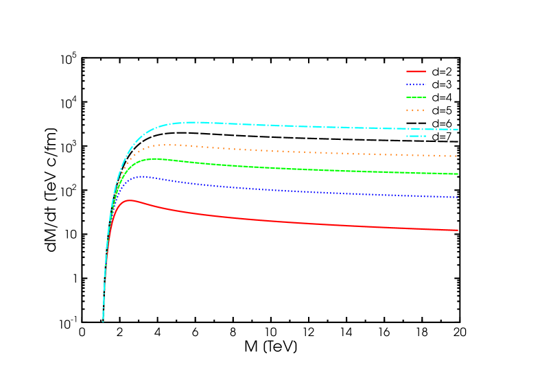
Figure 1: The evaporation rate Eq. (16) for various $d$ for $M_{\rm R}=M_{\rm f}=1$ TeV and the standard entropy, i.e. the parameter set Eq. (9). Here, Boltzmann- statistic was used.

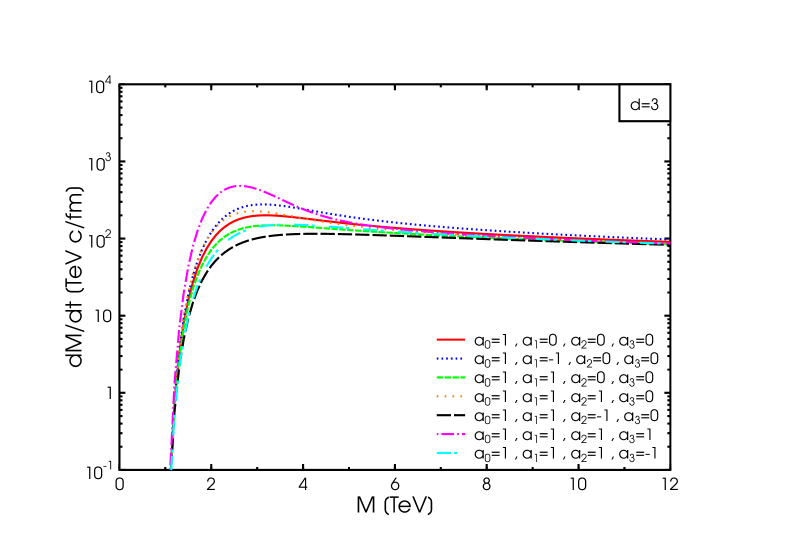
Figure 2: The evaporation rate for the black hole with $M_{\rm R}=M_{\rm f}=1$ TeV and $d=3$ for various parameters $a_{i}$. Here, Boltzmann-statistic was used.

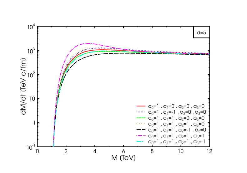
Figure 3: The evaporation rate for the black hole with $M_{\rm R}=M_{\rm f}=1$ TeV and $d=5$ for various parameters $a_{i}$. Here, Boltzmann-statistic was used.

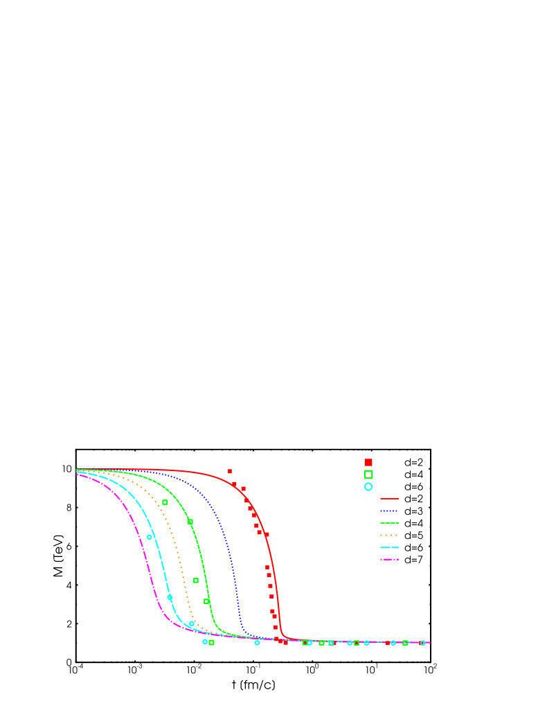
Figure 4: The mass evolution for a black hole of initial mass $M=10$ TeV and various $d$. Here, we set $M_{\rm R}=M_{\rm f}=1$ TeV. The full lines show the analytical calculation. The numerical results are shown as symbols. Note that each numerical example shows a single event only.

From the evaporation rate Eq.(16) one obtains by integration the mass evolution $M(t)$ of the black hole. This is shown for the continuous mass case in Figure 4. For a realistic scenario one has to take into account that the mass loss will proceed by steps by radiation into the various particles of the Standard Model.

Results

We have included the evaporation rate, parametrized according to the previous section, into the black hole event generator CHARYBDIS and examined the occurring observables within the PYTHIA environment. Since these black hole remnants are stable, they are of special interest as they are available for close investigations. Especially those remnants carrying an electric charge offer exciting possibilities as investigated in [55].

It has also been shown in [55] that no naked singularities have to be expected for reasonably charged black holes and that the modification of the Hawking radiation due to the electric charge can be neglected for the parameter ranges one expects at the LHC. This means in particular that the interaction of emitted charged particles with the black hole does not noticeably modify the emission probability. Although there might be uncertainties in the low energy limit where QED or QCD interactions might have unknown consequences for the processes at the horizon.

The formation of a remnant indeed solves a (technical) problem occuring within the treatment of a final decay: it might in principle have happened that during its evaporation process, the black hole has emitted mostly electrically charged particles and ended up with an electric charge of order ten. In such a state, it would then be impossible for the black hole to decay into less than ten particles of the SM, whereas the standard implementation allows only a decay into a maximum of 5 particles.

Therefore, in the original numerical treatment, the process of Hawking radiation has before been assumed to minimize the charge of the evaporating hole in each emission step. In such a way, it was assured that the object always had a small enough charge to enable the final decay in $\leq 5$ particles without any violation of conservation laws. This situation changes if the remnant is allowed to keep the electric charge. In the here presented analysis, the assumption of charge minimization has therefore been dropped as it is no longer necessary. However, we want to stress, that the in- or exclusion of charge minimization does not modify the observables investigated.

When attempting to investigate slowly decaying objects, one might be concerned whether these decay in the collision region or might be able to leave the detector, thereby still emitting radiation. As shown for the continuous case in Fig. 4, the average energy of the emitted particles drops below an observable range within a $10$ fm radius. Even if one takes into account the large $\gamma$-factor, the black hole will have shrunken to remnant-mass safely in the detector region. This is shown for a sample of simulated events in Fig. 4 (symbols) which displays the mass evolution of these collider produced black holes. Here, we estimated the time, $t$, for the stochastic emission of a quanta of energy $E$ to be $1/E$. This numerical result agrees very well with the expectations from the continuous case.

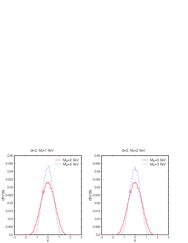
Figure 5: Rapidity distribution of the black hole remnants in pp interactions at $\sqrt{s}=14$ TeV for $d=2$. The curves for different number of extra dimensions $d$ differ from the depicted ones by less than 5% and are not shown.

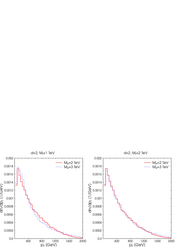
Figure 6: Transverse momentum distribution of the black hole remnants in pp interactions at $\sqrt{s}=14$ TeV.

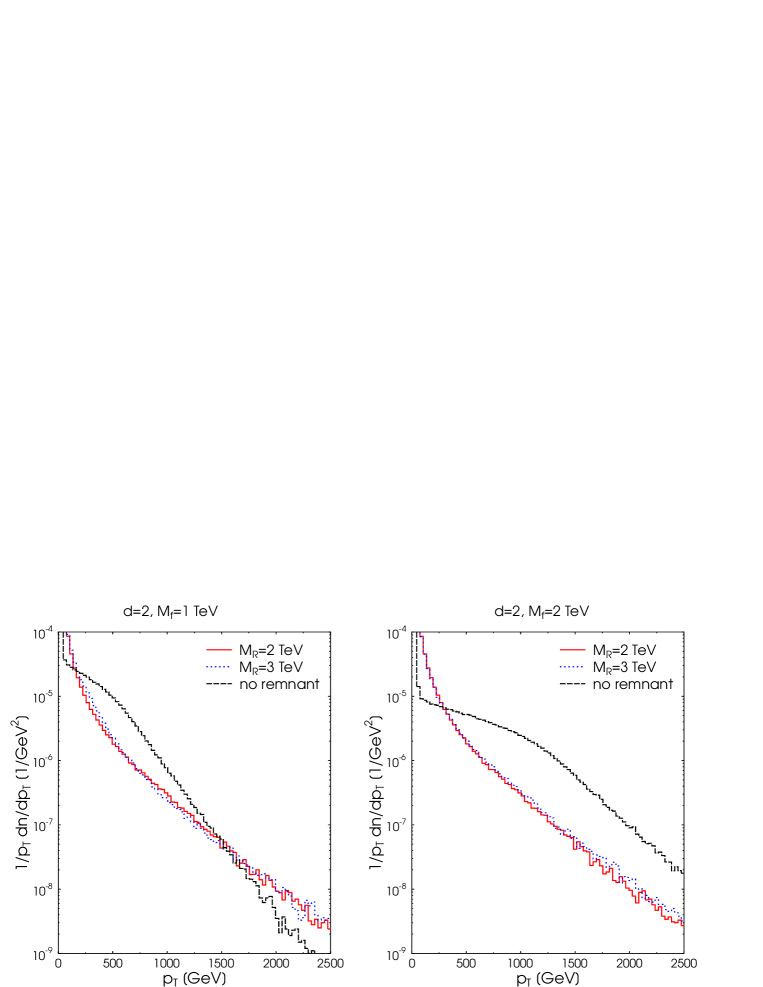
Figure 7: Transverse momentum distribution of initially emitted particles (i.e. before the fragmentation of the emitted partons) with final (two-body) decay in contrast to the formation of a black hole remnant.

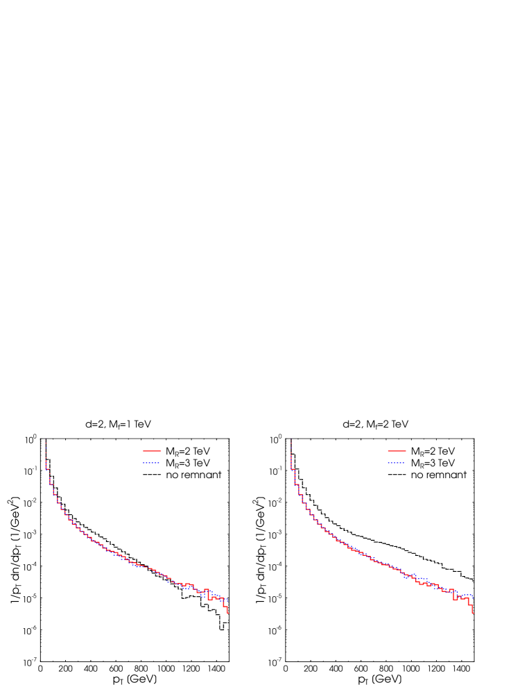
Figure 8: Transverse momentum distribution after fragmentation with final (two-body) decay in contrast to the formation of a black hole remnant.

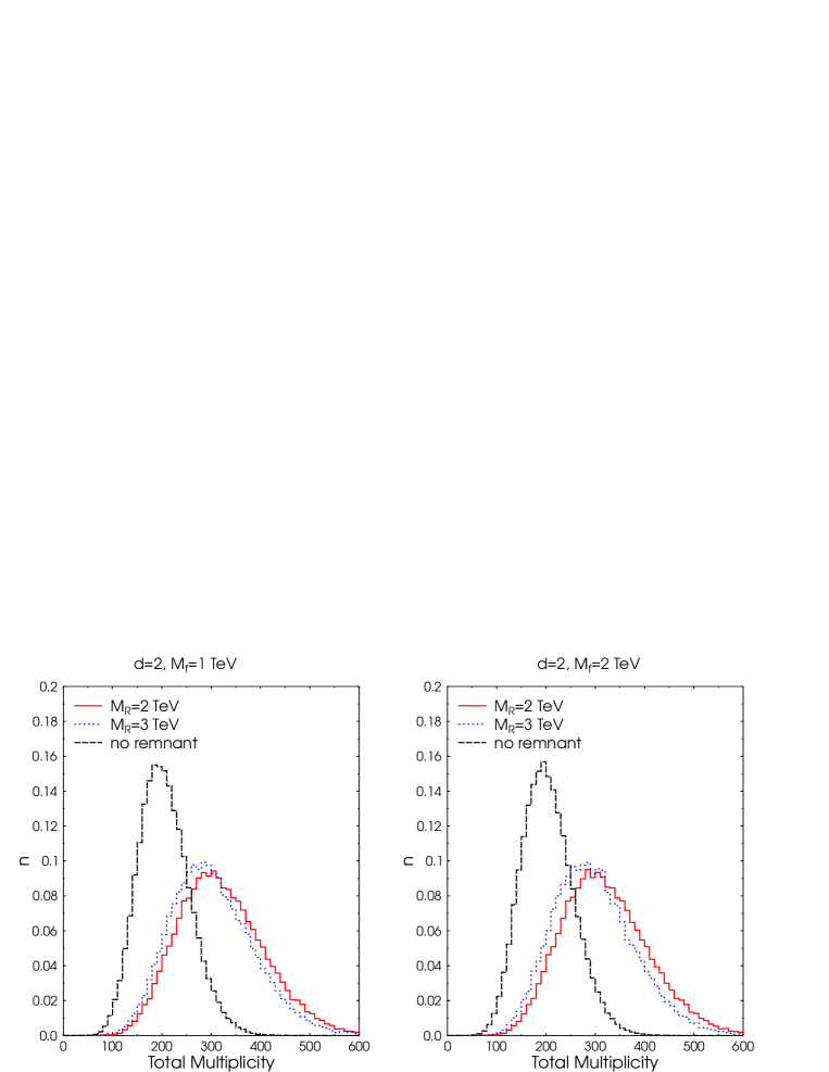
Figure 9: Total multiplicity with final (two-body) decay in contrast to the formation of a black hole remnant for $d=2$.

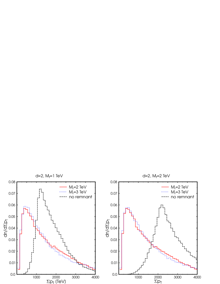
Figure 10: The total sum of the transverse momenta of the decay products.

To understand the fast convergence of the black hole mass, recall the spectral energy density which enters in Eq.(16) and which dictates the distribution of the emitted particles. Even though the spectrum is no longer an exactly Planckian, it still retains a maximum at energies $\sim 1/T$. If the black hole’s mass decreases, the emission of the high energetic end of the spectrum is no longer possible. For masses close to the Planck scale, the spectrum has a maximum at the largest possible energies that can be emitted. Thus, the black hole has a high probability to emit its remaining energy in the next emission process. However, theoretically, the equilibrium time goes to infinity (because the evaporation rate falls to zero, see Fig. 1) and the black hole will emit an arbitrary amount of very soft photons. For practical purposes, we cut off the evaporation when the black hole reached the mass $M_{\rm R}+0.1$ GeV.

Figure 5 shows the rapidity of the produced black hole remnants in a proton-proton collision at $\sqrt{s}=14$ TeV. All plots are for $d=2$ since a higher number of extra dimensions leads to variations of less than 5%. The reader should be aware that the present numerical studies assume the production of one black hole in every event. To obtain the absolute cross sections the calculated yields have to be multiplied by the black hole production cross section $\sigma({\rm pp}\rightarrow BH)$. Due to the uncertainties in the absolute production cross section of black holes we have taken this factor explicitely out. For the present examination we have initialized a sample of 50,000 events. The black hole remnants are strongly peaked around central rapidities, making them potentially accessible to the CMS and ATLAS experiments. In Figure 6 we show the distribution of the produced black hole remnants as a function of the transverse momentum.

Figure 7 shows the transverse momentum, $p_{T}$, of the decay products as it results from the modified multi particle number density Eq. (13) before fragmentation. Figure 8 shows the $p_{T}$-spectrum after fragmentation. In both cases, one clearly sees the additional contribution from the final decay which causes a bump in the spectrum which is absent in the case of a remnant formation. After fragmentation, this bump is slightly washed out but still present. However, from the rapidity distribution and the fact that the black hole event is spherical, a part of the high $p_{T}$-particles will be at large $y$ and thus be not available in the detector. We therefore want to mention that one has to include the experimental acceptance in detail if one wants to compare to experimental observables.

Figure 9 shows the total multiplicities of the event. When a black hole remnant is formed, the multiplicity is increased due to the additional low energetic particles that are emitted in the late stages instead of a final decay with $2-5$ particles. Note that this multiplicity increase is not an effect of the remnant formation itself, but stems from the treatment of the decay in the micro-canonical ensemble used in the present calculation. I.e. the black hole evaporates a larger amount of particles with lower average energy.

Figure 10 shows the sum over the transverse momenta of the black holes’ decay products. To interpret this observable one might think of the black hole event as a multi-jet with total $\Sigma p_{T}$. As is evident, the formation of a remnant lowers the total $\Sigma p_{T}$ by about $M_{\rm R}$. This also means, that the signatures of the black hole as previously analyzed are dominated by the daubtful final decay and not by the Hawking phase. It is interesting to note that the dependence on $M_{\rm f}$ is dominated by the dependence on $M_{\rm R}$, making the remnant mass the primary observable, leading to an increase in the missing energy.

5 Conclusion

We have parametrized the modifications to the black hole evaporation arising from the presence of a remnant mass. The modified spectral density is included in the numerical simulation for black hole events. To give a specific example, we have examined the formation of black hole remnants in proton proton collision at $\sqrt{s}=14$ TeV and set it in contrast to a final decay of the black hole.

We predict a significant decrease of the total transverse momentum of the black hole remnant events due to the absence of the final decay particles. Even more, the multiplicity of the event is increased by a factor $\sim 3/2$ arising from the micro-canonical treatment of the evaporation process.

The formation of the black hole remnant results in a strong modification of most predicted black hole signatures. However, remnant formation itself leads to prominent experimental signatures (see e.g. $\Sigma p_{T}$). This makes the search for black hole remnants promising and experimentally accessible for the CMS and ATLAS experiments.

References

- [1] N. Arkani-Hamed, S. Dimopoulos and G. R. Dvali, Phys. Lett. B 429, 263 (1998); I. Antoniadis, N. Arkani-Hamed, S. Dimopoulos and G. R. Dvali, Phys. Lett. B 436, 257 (1998); N. Arkani-Hamed, S. Dimopoulos and G. R. Dvali, Phys. Rev. D 59, 086004 (1999).
- [2] I. Antoniadis, Phys. Lett. B 246, 377 (1990).
- [3] I. Antoniadis and M. Quiros, Phys. Lett. B 392, 61 (1997).
- [4] K. R. Dienes, E. Dudas and T. Gherghetta, Nucl. Phys. B 537, 47 (1999). K. R. Dienes, E. Dudas and T. Gherghetta, Phys. Lett. B 436, 55 (1998).
- [5] P.C. Argyres, S. Dimopoulos, and J. March-Russell, Phys. Lett. B441, 96 (1998).
- [6] T. Banks and W. Fischler, arXiv:hep-th/9906038.
- [7] R. Emparan, G. T. Horowitz and R. C. Myers Phys. Rev. Lett. 85, 499 (2000).
- [8] S. Dimopoulos and G. Landsberg Phys. Rev. Lett. 87, 161602 (2001).
- [9] S. B. Giddings and S. Thomas, Phys. Rev. D 65 056010 (2002).
- [10] I. Mocioiu, Y. Nara and I. Sarcevic, Phys. Lett. B 557 (2003) 87; A. V. Kotwal and C. Hays, Phys. Rev. D 66 (2002) 116005; Y. Uehara, Prog. Theor. Phys. 107, 621 (2002); R. Emparan, M. Masip and R. Rattazzi, Phys. Rev. D 65, 064023 (2002); S. Hossenfelder, S. Hofmann, M. Bleicher and H. Stocker, Phys. Rev. D 66 (2002) 101502. A. Ringwald and H. Tu, Phys. Lett. B 525 (2002) 135; D. Kazanas and A. Nicolaidis, Gen. Rel. Grav. 35 (2003) 1117.
- [11] M. B. Voloshin, Phys. Lett. B 518, 137 (2001); Phys. Lett. B 524, 376 (2002).
- [12] S. B. Giddings, in Proc. of the APS/DPF/DPB Summer Study on the Future of Particle Physics (Snowmass 2001) ed. N. Graf, eConf C010630, P328 (2001).
- [13] S. N. Solodukhin, Phys. Lett. B 533, 153 (2002).
- [14] A. Jevicki and J. Thaler, Phys. Rev. D 66, 024041 (2002); T. G. Rizzo, in Proc. of the APS/DPF/DPB Summer Study on the Future of Particle Physics (Snowmass 2001) ed. N. Graf, eConf C010630, P339 (2001); D. M. Eardley and S. B. Giddings, Phys. Rev. D 66, 044011 (2002).
- [15] I. Ya. Yref’eva, Part.Nucl. 31, 169-180 (2000). S. B. Giddings and V. S. Rychkov, Phys. Rev. D 70, 104026 (2004); V. S. Rychkov, [arXiv:hep-th/0410041]; O. V. Kancheli, [arXiv:hep-ph/0208021].
- [16] G. T. Horowitz and J. Polchinski, Phys. Rev. D 66 103512 (2002).
- [17] H. Yoshino and Y. Nambu, Phys. Rev. D 67, 024009 (2003).
- [18] L. Anchordoqui and H. Goldberg, Phys. Rev. D 67, 064010 (2003); K. Cheung, Phys. Rev. D 66, 036007 (2002); K. m. Cheung, Phys. Rev. Lett. 88, 221602 (2002); S. C. Park and H. S. Song, J. Korean Phys. Soc. 43, 30 (2003); S. Hossenfelder, S. Hofmann, M. Bleicher and H. Stocker, Phys. Rev. D 66, 101502 (2002); M. Bleicher, S. Hofmann, S. Hossenfelder and H. Stocker, Phys. Lett. B 548, 73 (2002); M. Cavaglia, S. Das and R. Maartens, Class. Quant. Grav. 20, L205 (2003); M. Cavaglia and S. Das, Class. Quant. Grav. 21, 4511 (2004); S. Hossenfelder, Phys. Lett. B 598, 92 (2004); A. Ringwald, Fortsch. Phys. 51, 830 (2003);A. Chamblin and G. C. Nayak, Phys. Rev. D 66, 091901 (2002).
- [19] V. S. Rychkov, Phys. Rev. D 70, 044003 (2004); K. Kang and H. Nastase, [arXiv:hep-th/0409099]. V. S. Rychkov, arXiv:hep-th/0410295. H. Yoshino and V. S. Rychkov, Phys. Rev. D 71 (2005) 104028 [arXiv:hep-th/0503171].
- [20] V. Cardoso, E. Berti and M. Cavaglia, Class. Quant. Grav. 22 (2005) L61 [arXiv:hep-ph/0505125].
- [21] P. Kanti, Int. J. Mod. Phys. A 19 (2004) 4899. G. Landsberg, [arXiv:hep-ph/0211043]; M. Cavaglia, Int. J. Mod. Phys. A 18, 1843 (2003); S. Hossenfelder, in ’Focus on Black Hole Research’, edited by P. V. Kreitler, Novapublishers (2005), [arXiv:hep-ph/0412265].
- [22] S. W. Hawking, Comm. Math. Phys. 43, 199-220 (1975); Phys. Rev. D 14, 2460-2473 (1976).
- [23] C. M. Harris, P. Richardson and B. R. Webber, JHEP 0308, 033 (2003) [arXiv:hep-ph/0307305].
- [24] J. Tanaka, T. Yamamura, S. Asai and J. Kanzaki, [arXiv:hep-ph/0411095].
- [25] C. M. Harris, M. J. Palmer, M. A. Parker, P. Richardson, A. Sabetfakhri and B. R. Webber, [arXiv:hep-ph/0411022].
- [26] K. Cheung, [arXiv:hep-ph/0409028]; G. Landsberg, [arXiv:hep-ex/0412028].
- [27] R. C. Myers and M. J. Perry Ann. Phys. 172, 304-347 (1986).
- [28] T. G. Rizzo, [arXiv:hep-ph/0503163]; T. G. Rizzo, [arXiv:hep-ph/0504118].
- [29] R. M. Wald, Phys. Rev. D 56, 6467 (1997), [arXiv:gr-qc/9704008].
- [30] T. Sjostrand, L. Lonnblad and S. Mrenna, [arXiv:hep-ph/0108264].
- [31] I. D. Novikov and V. P. Frolov, ”Black Hole Physics”, Kluver Academic Publishers (1998).
- [32] S. Hawking, Commun. Math. Phys. 87,395 (1982).
- [33] J. Preskill, [arXiv:hep-th/9209058].
- [34] D. N. Page, Phys. Rev. Lett. 44, 301 (1980); G. t’Hooft, Nucl. Phys. B 256 727 (1985); A. Mikovic, Phys. Lett. 304 B, 70 (1992); E. Verlinde and H. Verlinde, Nucl. Phys. B 406, 43 (1993); L. Susskind, L. Thorlacius and J. Uglum, Phys. Rev. D 48, 3743 (1993); D. N. Page, Phys. Rev. Lett. 71 3743 (1993).
- [35] Y. Aharonov, A. Casher and S. Nussinov, Phys. Lett. 191 B, 51 (1987); T. Banks, A. Dabholkar, M. R. Douglas and M. O’Loughlin, Phys. Rev. D 45 3607 (1992), [arXiv:hep-th/9201061]; T. Banks and M. O’Loughlin, Phys. Rev. D 47, 540 (1993), [arXiv:hep-th/9206055]; T. Banks, M. O’Loughlin and A. Strominger, Phys. Rev. D 47, 4476 (1993), [arXiv:hep-th/9211030]; S. B. Giddings, Phys. Rev. D 49, 947 (1994), [arXiv:hep-th/9304027]. M. D. Maia, [arXiv:gr-qc/0505119]; V. Husain and O. Winkler, [arXiv:gr-qc/0505153].
- [36] M. A. Markov, in: ”Proc. 2nd Seminar in Quantum Gravity”, edited by M. A. Markov and P. C. West, Plenum, New York (1984).
- [37] Y. B. Zel’dovich, in: ”Proc. 2nd Seminar in Quantum Gravity”, edited by M. A. Markov and P. C. West, Plenum, New York (1984).
- [38] R. J. Adler, P. Chen and D. I. Santiago, Gen. Rel. Grav. 33, 2101 (2001) [arXiv:gr-qc/0106080].
- [39] K. Nozari and S. H. Mehdipour, [arXiv:gr-qc/0504099].
- [40] J. D. Barrow, E. J. Copeland and A. R. Liddle, Phys. Rev. D 46, 645 (1992).
- [41] B. Whitt, Phys. Rev. D 38, 3000 (1988).
- [42] R. C. Myers and J. Z. Simon, Phys. Rev. D 38, 2434 (1988).
- [43] C. G. Callan, R. C. Myers and M. J. Perry, Nucl. Phys. B 311, 673 (1988).
- [44] S. Alexeyev, A. Barrau, G. Boudoul, O. Khovanskaya and M. Sazhin, Class. Quant. Grav. 19, 4431-4444 (2002), [arXiv:gr-qc/0201069]
- [45] M. J. Bowick, S. B. Giddings, J. A. Harvey, G. T. Horowitz and A. Strominger, Phys. Rev. Lett. 61 2823 (1988).
- [46] S. Coleman, J. Preskill and F. Wilczek, Mod. Phys. Lett. A6 1631 (1991).
- [47] K-Y. Lee, E. D. Nair and E. Weinberg, Phys. Rev. Lett. 68 1100 (1992).
- [48] G. W. Gibbons and K. Maeda, Nucl. Phys. B 298 741 (1988).
- [49] T. Torii and K. Maeda, Phys. Rev. D 48 1643 (1993).
- [50] S. Hossenfelder, M. Bleicher, S. Hofmann, H. Stocker and A. V. Kotwal, Phys. Lett. B 566, 233 (2003), [arXiv:hep-ph/0302247].
- [51] R. Casadio and B. Harms, Phys.Rev. D 64, 024016 (2001) [arXiv:hep-th/0101154]; Phys.Lett. B 487 209-214 (2000) [arXiv:hep-th/0004004]; D. N. Page, Phys. Rev. D 13 198 (1976).
- [52] P. Kraus and F. Wilczek, Nucl. Phys. B 433, 403 (1995) [arXiv:gr-qc/9408003]; P. Kraus and F. Wilczek, Nucl. Phys. B 437, 231 (1995) [arXiv:hep-th/9411219]; E. Keski-Vakkuri and P. Kraus, Nucl. Phys. B 491, 249 (1997) [arXiv:hep-th/9610045]; S. Massar and R. Parentani, Nucl. Phys. B 575, 333 (2000) [arXiv:gr-qc/9903027]; T. Jacobson and R. Parentani, Found. Phys. 33, 323 (2003) [arXiv:gr-qc/0302099].
- [53] M. K. Parikh and F. Wilczek, Phys. Rev. Lett. 85, 5042 (2000) [arXiv:hep-th/9907001].
- [54] A. J. M. Medved and E. C. Vagenas, [arXiv:gr-qc/0504113]; M. Arzano, [arXiv:hep-th/0504188].
- [55] S. Hossenfelder, B. Koch and M. Bleicher, [arXiv:hep-ph/0507140].