2005 International Linear Collider Workshop - Stanford, U.S.A.
Split Supersymmetry at Colliders

Abstract

We consider the collider phenomenology of split-supersymmetry models. Despite the challenging nature of the signals in these models the long-lived gluino can be discovered with masses above $2\,{\rm\,TeV}$ at the LHC. At a future linear collider we will be able to observe the renormalization group effects from split supersymmetry on the chargino/neutralino mixing parameters, using measurements of the neutralino and chargino masses and cross sections. This indirect determination of chargino/neutralino anomalous Yukawa couplings is an important check for supersymmetric models in general.

I INTRODUCTION

Split supersymmetry SpS is a possibility to evade many of the phenomenological constraints that plague generic supersymmetric extensions of the Standard Model. By splitting the supersymmetry-breaking scale between the scalar and the gaugino sector, the squarks and sleptons are rendered heavy (somewhere between several ${\rm\,TeV}$ and the GUT scale), while charginos and neutralinos may still be at the ${\rm\,TeV}$ scale or below. This setup eliminates dangerous flavor-changing neutral current transitions, electric dipole moments, and spurious proton-decay operators without the need for mass degeneracy between the sfermion generations. The benefits of the supersymmetry paradigm, in particular the unification of gauge groups at a high scale and the successful dark-matter prediction, are retained.

In the Higgs sector, the split-supersymmetry scenario requires a fine-tuning that pulls the Higgs vacuum expectation value down to the observed electroweak scale. The extra Higgses of a supersymmetric model are located at the sfermion mass scale. This fine-tuning is obviously unnatural, but it may (or may not) find a convincing explanation in ideas beyond the realm of particle physics landscape ; drees .

In this talk (for more details, see pheno ), we investigate the split-supersymmetry scenario from a purely phenomenological point of view. We ask ourselves the question whether and how (i) the particles present in the low-energy spectrum can be detected, and (ii) the underlying supersymmetric nature of the model can be verified. The two tasks require combining LHC and ILC data.

The low-energy effective theory is particularly simple. In addition to the Standard Model spectrum including the Higgs boson, the only extra particles are the four neutralinos, two charginos, and a gluino. Since all squarks are very heavy, the gluino is long-lived. The gluino can be produced at the LHC only, while the charginos and neutralinos can be accessible both at the LHC and at the ILC.

Renormalization group running without sfermions and heavy Higgses lifts the light Higgs mass considerably above the LEP limit, solving another problem of the MSSM. Still, the Higgs boson is expected to be lighter than about $200{\rm\,GeV}$. Apart from this Higgs mass bound, the only trace of supersymmetry would be the mutual interactions of Higgses, gauginos, and Higgsinos, i.e., the chargino and neutralino Yukawa couplings. These couplings are determined by the gauge couplings at the matching scale $\widetilde{m}$, where the scalars are integrated out.

II RENORMALIZATION GROUP EVOLUTION

Although, in the absence of sfermions, the overall phenomenology of split-supersymmetry models does not depend very much on the particular spectrum, for a quantitative analysis we have to select a specific scenario. To this end, we note that the popular assumption of radiative symmetry breaking (i.e., a common scalar mass parameter for sfermions and Higgses) has to be dropped, and the Higgsino mass parameter $\mu$ is an independent quantity. Assuming gauge coupling unification and gaugino mass unification, we start from the following model parameters at the grand unification scale $M_{\rm GUT}=6\times 10^{16}{\rm\,GeV}$:

$$M_{1}(M_{\rm GUT})=M_{2}(M_{\rm GUT}) =M_{3}(M_{\rm GUT})=120{\rm\,GeV}, \mu(M_{\rm GUT}) =-90{\rm\,GeV}, \tan\beta =4.$$ (1)

For the SUSY-breaking scale we choose $\widetilde{m}=10^{9}{\rm\,GeV}$. Figure 1 displays the solutions of the renormalization group equations with the input parameters set in eq.(1) pheno . At the low scale $Q=m_{Z}$, we extract the mass parameters:

$$M_{1}(Q=m_{Z}) =74.8{\rm\,GeV} \qquad\qquad M_{3}^{\overline{\text{DR}}}(Q=1{\rm\,TeV}) =690.1{\rm\,GeV}$$

$$M_{2}(Q=m_{Z}) =178.1{\rm\,GeV} \qquad\qquad\mu(Q=m_{Z}) =-120.1{\rm\,GeV}$$ (2)

The resulting physical gaugino and Higgsino masses are:

$$m_{\tilde{\chi}^{0}_{1}} =71.1{\rm\,GeV}, m_{\tilde{\chi}^{0}_{2}} =109.9{\rm\,GeV}, m_{\tilde{\chi}^{0}_{3}} =141.7{\rm\,GeV}, m_{\tilde{\chi}^{0}_{4}} =213.7{\rm\,GeV},$$

$$m_{\tilde{\chi}^{+}_{1}} =114.7{\rm\,GeV}, m_{\tilde{\chi}^{+}_{2}} =215.7{\rm\,GeV}, m_{\tilde{g}} =807{\rm\,GeV}$$ (3)

These mass values satisfy the LEP constraints. Virtual effects of a split supersymmetry spectrum on Standard Model observables have recently been discussed in Martin:2004id .

The neutralinos $\tilde{\chi}^{0}_{1,2,3,4}$ are predominantly bino, Higgsino, Higgsino, and wino, respectively. The Higgsino content of the lightest neutralino is $h_{f}=0.2$, so the dark-matter condition dm is satisfied. To our given order the Higgs mass is $m_{H}=150{\rm\,GeV}$.

Figure 1: Renormalization group flow of the gauge couplings (left), the gaugino–Higgsino mass parameters (centre), and the anomalous gaugino–Higgsino mixing parameters defined in eq.(4) (right). All curves are based on our reference point eq.(2).

Because we integrate out the heavy scalars, the neutralino and chargino Yukawa couplings deviate from their usual MSSM prediction, parameterized by four anomalous Yukawa couplings $\kappa$. We can extract their weak-scale values from Fig. 1:

$$\frac{\tilde{g}_{u}}{g\sin\beta} \equiv 1+\kappa_{u}=1+0.018 \frac{\tilde{g}_{d}}{g\cos\beta} \equiv 1+\kappa_{d}=1+0.081$$

$$\frac{\tilde{g}^{\prime}_{u}}{g^{\prime}\sin\beta} \equiv 1+\kappa^{\prime}_{u}=1-0.075 \frac{\tilde{g}^{\prime}_{d}}{g^{\prime}\cos\beta} \equiv 1+\kappa^{\prime}_{d}=1-0.17$$ (4)

III LONG-LIVED GLUINOS

Since the standard cascade decays of initial squarks and gluinos are absent in this model, there are only two sources of new particles left. The gluino is produced in pairs from gluon-gluon and quark-antiquark annihiliation. Pairs of charginos and neutralinos are produced through a Drell–Yan $s$-channel $Z$ boson, photon, or $W$ boson. These cross sections are known to next-to-leading order precision LHC-NLO .

Unless we have a-priori knowledge about the sfermion scale $\widetilde{m}$, the gluino lifetime is undetermined. Figure 2 compares this scale with other relevant scales of particle physics. Once $\widetilde{m}\gtrsim 10^{3}{\rm\,GeV}$, the gluino hadronizes before decaying. The resulting states that consist of either of a gluino and pairs or triplets of quarks, or of a gluino bound to a gluon, are called $R$-hadrons Rhadrons . For gluinos produced near threshold, the formation of gluino-pair bound states (gluinonium) is also possible and leads to characteristic signals gluinonium .

For $\widetilde{m}>10^{6}{\rm\,GeV}$, the gluino travels a macroscopic distance. If $\widetilde{m}>10^{7}{\rm\,GeV}$, strange $R$-hadrons can also decay weakly, and gluinos typically leave the detector undecayed or are stopped in the material. For even higher scales, $\widetilde{m}>10^{9}{\rm\,GeV}$, $R$-hadrons could become cosmologically relevant, since they affect nucleosynthesis if their abundance in the early Universe is sufficiently high SpS .

Figure 2: Gluino lifetime Muhlleitner:2003vg as a function of the common scalar mass $\widetilde{m}$.

If gluino decays can be observed, their analysis yields information about physics at the scale $\widetilde{m}$ and thus allows us to draw conclusions about the mechanism of supersymmetry breaking gldecay .

Without relying on gluino decays, there are two strategies for detecting the corresponding $R$-hadrons pheno ; Hewett:2004nw . (i) The production of a stable, charged, $R$-hadron will give a signal much like the production of a stable charged weakly-interacting particle. This signal consists of an object that looks like a muon but arrives at the muon chambers significantly later than a muon owing to its large mass. (ii) While for stable neutral $R$-hadrons there will be some energy loss in the detector, there will be a missing transverse energy signal due to the escape of the $R$-hadrons. As leptons are unlikely to be produced in this process, the signal will be the classic SUSY jets with missing transverse energy signature.

In Fig. 3, we show the expected discovery reach for both channels, based on models for the $R$-hadron spectrum and the $R$-hadron interaction in the detector that we have implemented in HERWIG HERWIG .

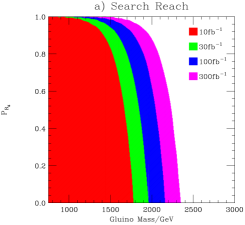
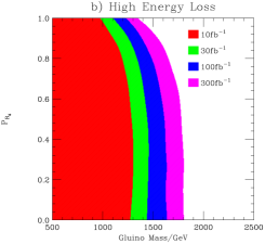
Figure 3: Gluino discovery reach at the LHC for (a) charged $R$-hadrons, (b) neutral $R$-hadrons, from pheno .

IV CHARGINO AND NEUTRALINO YUKAWA COUPLINGS

If split supersymmetry should be realized in nature, the observation of the gluino, charginos and neutralinos will only be the first task. Once these states are discovered, we will have to show that at the scale $\widetilde{m}$ they constitute a supersymmetric Lagrangian.

A quantitative trace of this is given by the off-diagonal elements in the mass matrices that derive from the gaugino-higgsino-Higgs couplings (4). They determine the mixing of gauginos and higgsinos into charginos and neutralinos as mass eigenstates. Simultaneously, they also constitute the neutralino and chargino Yukawa couplings. In split supersymmetry, the renormalization flow below the sfermion scale $\widetilde{m}$ induces non-zero values of order $\kappa^{(\prime)}_{i}=-0.2\ldots 0.2$. If we are able to detect deviations of this size at a collider, we can both establish the supersymmetric nature of the model and verify the matching condition to the MSSM at $\widetilde{m}$.

To measure the neutralino and chargino mixing matrices, a precise mass measurement is necessary. This is possible (for mass differences, at least) at the LHC and, to a better accuracy, at the ILC. Without gaugino–Higgsino mixing the mass matrices would be determined by the MSSM parameters $M_{1},M_{2}$ and $\mu$. The gaugino–Higgsino mixing adds terms of the order of $M_{Z}$ and introduces the additional parameter $\tan\beta$, leading to four MSSM parameters altogether.

In $e^{+}e^{-}$ collisions, for the parameter set (2) almost all chargino and neutralino production channels have cross sections larger than $0.1{\rm\,fb}$, and the threshold value for $\tilde{\chi}^{+}_{1}\tilde{\chi}^{-}_{1}$ production is as large as $1\;{\rm\,pb}$ pheno . The NLO electroweak corrections to these production cross sections have been calculated in ILC-NLO . A linear collider with moderate energy and high luminosity would be optimal to probe all these processes, and some kind of fit is the proper method to extract the weak-scale Lagrangian parameters.

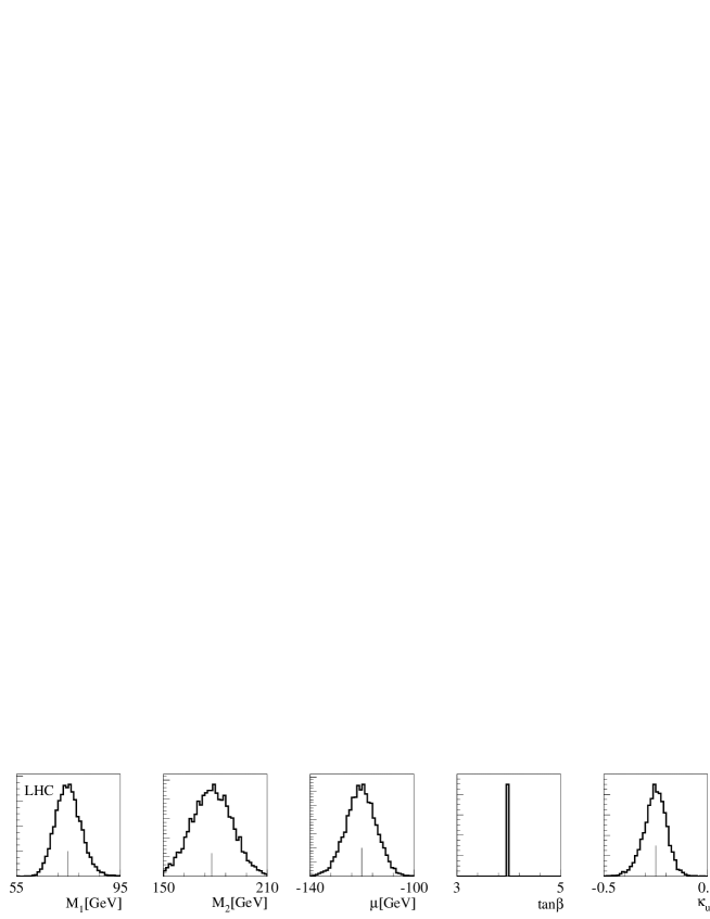
Figure 4: Fit to 10000 sets of mass and cross section pseudo-measurements at the LHC (upper) and at the ILC (lower). The fitted parameters include only $\kappa_{u}$ with a central value zero. At the LHC $\tan\beta=4$ is fixed.

Figure 5: Fit to 10000 sets of mass and cross section pseudo-measurements at a future linear collider. All four $\kappa^{(\prime)}_{i}$ are extracted simultaneously. The central values are set to the example split supersymmetry values. The MSSM zero prediction is indicated in the lower line of histograms.

We compute the masses and the cross sections for all pair-production processes, with the exception of the $\tilde{\chi}^{0}_{1}\tilde{\chi}^{0}_{1}$ channel. To all observables we assign an experimental error, which in our simplified treatment is a relative error of $0.5\%$ on all linear-collider mass measurements Aguilar-Saavedra:2001rg , $5\%$ on all LHC mass measurements Bachacou:1999zb , and the statistical uncertainty on the number of events at a linear collider corresponding to $100{\rm\,fb}^{-1}$ of data at a $1{\rm\,TeV}$ collider after all efficiencies.

	Fit $\tan\beta$	$m_{i}$	$\sigma_{ij}$	$\Delta\kappa_{u}$	$\Delta\kappa_{d}$	$\Delta\kappa^{\prime}_{u}$	$\Delta\kappa^{\prime}_{d}$
Tesla		$\bullet$	$\bullet$	$0.9\times 10^{-2}$	$3\times 10^{-2}$	$1.3\times 10^{-2}$	$4\times 10^{-2}$
Tesla	$\bullet$	$\bullet$	$\bullet$	$1.2\times 10^{-2}$	$5\times 10^{-2}$	$2\times 10^{-2}$	$5\times 10^{-2}$
Tesla		$\bullet$		$1.1\times 10^{-2}$	$5\times 10^{-2}$	$3\times 10^{-2}$	$8\times 10^{-2}$
Tesla	$\bullet$	$\bullet$		$1.2\times 10^{-2}$	$11\times 10^{-2}$	$4\times 10^{-2}$	$8\times 10^{-2}$
LHC		$\bullet$		$2.2\times 10^{-1}$	$6\times 10^{-1}$	$2.7\times 10^{-1}$	$8\times 10^{-1}$
Tesla		$\bullet$	$\bullet$	$1.4\times 10^{-2}$	$5\times 10^{-2}$	$3\times 10^{-2}$	$10\times 10^{-2}$
Tesla	$\bullet$	$\bullet$	$\bullet$	$1.7\times 10^{-2}$	$9\times 10^{-2}$	$4\times 10^{-2}$	$13\times 10^{-2}$
Tesla	fix $\tan\beta=3$	$\bullet$	$\bullet$	$1.6\times 10^{-2}$	$4\times 10^{-2}$	$4\times 10^{-2}$	$9\times 10^{-2}$
Tesla∗	$\kappa_{i}\neq 0$	$\bullet$	$\bullet$	$1.4\times 10^{-2}$	$5\times 10^{-2}$	$4\times 10^{-2}$	$11\times 10^{-2}$

Table 1: Error on the determination of $\kappa_{i}$ from measured masses and possibly production cross sections. For the first five lines, all but one $\kappa$ are fixed to zero, the fitted $\kappa$ has the central value zero. In the last four lines, all four $\kappa_{i}$ are fitted simultaneously. The very last line assumes the predicted central values of $\kappa_{i}$ in our parameter point.

Around the central parameter point we randomly generate 10000 sets of pseudo-measurements, using a Gaussian smearing. Out of each of these sets we extract the MSSM parameters by a global fit method. The fit results (see Fig. 4, top) show that at the LHC we can extract the Lagrangian mass parameters with reasonable precision. There is sensitivity to one Higgs-sector parameter, which we can take either as $\tan\beta$ or as one of the mixing parameters. If we fix $\tan\beta=4$, the precision on $\kappa_{u}$ is sufficient to verify consistency with a supersymmetric underlying theory. However, using LHC data alone, a simultaneous fit of all parameters gives only very weak constraints on the anomalous Yukawa couplings (Tab. 1), so no conclusions about the split-supersymmetry renormalization effects can be drawn.

The higher precision of measurements at the ILC, in particular adding cross sections as independent observables, allows us to improve the precision on a five-parameter fit (Fig. 4, bottom) or to simultaneously fit all Lagrangian parameters (Fig. 5). This is the proper treatment, unless we would have reasons to believe that some of the $\kappa^{(\prime)}_{i}$ are predicted to be too small to be measured. The results for the precision in determining the anomalous couplings are listed in Tab. 1. (Note that in a complete fit, $\tan\beta$ is no longer an independent parameter, so we can fix it to some given value.)

These results for the linear collider indeed indicate that we could not only confirm that the Yukawa couplings and the neutralino and chargino mixing follow the predicted MSSM pattern; for the somewhat larger $\kappa^{\prime}_{i}$ values we can even distinguish the complete weak-scale MSSM from a split supersymmetry spectrum.

While the elements of the neutralino and chargino mixing matrices depend on the Yukawa couplings in a complicated way, the cross sections for chargino/neutralino pair production in association with a Higgs boson are directly proportional to these parameters. Decays of the kind $\chi^{\pm}_{2}\to\chi^{\pm}_{1}H$ or $\chi^{0}_{j}\to\chi^{0}_{i}H$ would carry the same information, but typically are kinematically forbidden in split supersymmetry scenarios.

Associated production of charginos and neutralinos with a Higgs boson in the continuum can in principle be observed at a high-luminosity $e^{+}e^{-}$ collider. The cross sections for some of these channels exceed $0.1\;{\rm\,fb}$ with little background pheno , so with $1\;{\rm\,ab}^{-1}$ of luminosity we would expect some events of this kind to be detectable. However, due to the small rates for these processes, the achievable precision for parameter determination is limited. The measurement of masses and pair-production cross sections will be the key for establishing split supersymmetry as the underlying physical scenario.

- (1) N. Arkani-Hamed and S. Dimopoulos, arXiv:hep-th/0405159; G. F. Giudice and A. Romanino, Nucl. Phys. B 699, 65 (2004) [Erratum-ibid. B 706, 65 (2005)] [arXiv:hep-ph/0406088]; N. Arkani-Hamed, S. Dimopoulos, G. F. Giudice and A. Romanino, Nucl. Phys. B 709, 3 (2005) [arXiv:hep-ph/0409232]; J. D. Wells, Phys. Rev. D 71, 015013 (2005) [arXiv:hep-ph/0411041]; J. L. Feng and F. Wilczek, arXiv:hep-ph/0507032; S. Dimopoulos, these Proceedings.
- (2) L. Susskind, arXiv:hep-th/0302219; M. R. Douglas, arXiv:hep-th/0405279; N. Arkani-Hamed, S. Dimopoulos and S. Kachru, arXiv:hep-th/0501082.
- (3) M. Drees, arXiv:hep-ph/0501106.
- (4) W. Kilian, T. Plehn, P. Richardson and E. Schmidt, Eur. Phys. J. C 39, 229 (2005) [arXiv:hep-ph/0408088].
- (5) M. A. Diaz and P. F. Perez, J. Phys. G 31, 563 (2005) [arXiv:hep-ph/0412066]; S. P. Martin, K. Tobe and J. D. Wells, Phys. Rev. D 71, 073014 (2005) [arXiv:hep-ph/0412424].
- (6) A. Pierce, Phys. Rev. D 70, 075006 (2004) [arXiv:hep-ph/0406144].
- (7) W. Beenakker, R. Höpker, M. Spira and P. M. Zerwas, Nucl. Phys. B 492, 51 (1997); W. Beenakker, M. Klasen, M. Krämer, T. Plehn, M. Spira and P. M. Zerwas, Phys. Rev. Lett. 83, 3780 (1999); Prospino2.0, http://pheno.physics.wisc.edu/plehn
- (8) G. R. Farrar and P. Fayet, Phys. Lett. B 76, 575 (1978).
- (9) J. H. Kühn and S. Ono, Phys. Lett. B 142, 436 (1984); T. Goldman and H. Haber, Physica 15D, 181 (1985); I. I. Y. Bigi, V. S. Fadin and V. A. Khoze, Nucl. Phys. B 377, 461 (1992); E. Chikovani, V. Kartvelishvili, R. Shanidze and G. Shaw, Phys. Rev. D 53, 6653 (1996); [arXiv:hep-ph/9602249]. K. Cheung and W. Y. Keung, Phys. Rev. D 71, 015015 (2005) [arXiv:hep-ph/0408335].
- (10) J. L. Hewett, B. Lillie, M. Masip and T. G. Rizzo, JHEP 0409, 070 (2004) [arXiv:hep-ph/0408248].
- (11) M. Mühlleitner, A. Djouadi and Y. Mambrini, arXiv:hep-ph/0311167.
- (12) M. Toharia and J. D. Wells, arXiv:hep-ph/0503175; P. Gambino, G. F. Giudice and P. Slavich, arXiv:hep-ph/0506214; A. Arvanitaki, S. Dimopoulos, A. Pierce, S. Rajendran and J. Wacker, arXiv:hep-ph/0506242.
- (13) G. Corcella et al., JHEP 0101, 010 (2001); G. Corcella et al., arXiv:hep-ph/0210213.
- (14) W. Kilian, LC-TOOL-2001-039; W. Kilian, Proc. ICHEP 2002, Amsterdam; M. Moretti, T. Ohl and J. Reuter, arXiv:hep-ph/0102195; http://www-ttp.physik.uni-karlsruhe.de/whizard
- (15) W. Oller, H. Eberl and W. Majerotto, Phys. Lett. B 590, 273 (2004); T. Fritzsche and W. Hollik, arXiv:hep-ph/0407095.
- (16) J. A. Aguilar-Saavedra et al. [ECFA/DESY LC Physics Working Group Collaboration], arXiv:hep-ph/0106315; B. C. Allanach, G. A. Blair, S. Kraml, H. U. Martyn, G. Polesello, W. Porod and P. M. Zerwas, arXiv:hep-ph/0403133.
- (17) H. Bachacou, I. Hinchliffe and F. E. Paige, Phys. Rev. D 62, 015009 (2000); [arXiv:hep-ph/9907518]. B. C. Allanach, C. G. Lester, M. A. Parker and B. R. Webber, JHEP 0009, 004 (2000). [arXiv:hep-ph/0007009].