Competition of color ferromagnetic and superconductive states in a quark-gluon system

Abstract

The possibility of color ferromagnetism in an $SU(2)$ gauge field model is investigated. The conditions allowing a stable color ferromagnetic state of the quark system in the chromomagnetic field occupying small domains are considered. A phase transition between this state and the color superconducting states is considered. The effect of finite temperature is analyzed.

Introduction

Nonperturbative effects of non-abelian gauge theories take place in the infrared region. Among such nonperturbative effects are the existence of the QCD vacuum with gluon and quark condensates, chiral symmetry breaking, confinement and the hadronization process. They can only be studied by approximate methods and in the framework of various effective models. For instance, one of the possibilities to approximately describe the gluon condensate is to introduce background color fields of certain configurations (see, e.g., 5 ; 6 ).

Another example of nonperturbative problems is the physics of light mesons that can be described by effective four-fermion models such as the Nambu–Jona–Lasinio (NJL) quark model, which was successfully used to implement the ideas of dynamical chiral symmetry breaking ($D\chi SB$) and bosonization (see e.g. EbPerv ,7 and references therein; for a review of (2+1)-dimensional four-quark effective models see echaya ).

In the framework of four–fermion models, it was shown that a constant magnetic field 10 induces the dynamical chiral symmetry breaking ($D\chi SB$), as well as the fermion mass generation, even under conditions when the interaction between fermions is weak. This phenomenon of magnetic catalysis was explained basing upon the idea of effective reduction of space dimensionality in the presence of a strong external magnetic field 11 (see also paper 12 and references therein). It was also demonstrated that a strong chromomagnetic field catalyzes $D\chi SB$ 13 . As was shown in zheb , this effect can be understood in the framework of the dimensional reduction mechanism as well, and it does not depend on the particular form of the constant chromomagnetic field configuration.

One of the solutions of the Yang-Mills equations that can serve as a model for the gluon condensate is a constant chromomagnetic field. Its role was demonstrated in savv ; Matinyan . In these papers, the authors calculated the one-loop effective potential for a constant chromomagnetic field $B$ and they demonstrated that it reaches its minimum at a nonvanishing value of $B$.

However this simple analytical model of the gluon condensate with a uniform chromomagnetic field $B=\mbox{const}$ (the so-called “colour ferromagnetic state”) savv ; Matinyan suffered from an instability nielsen . This problem later has been studied in a number of papers. In particular, various methods were proposed to stabilize the solution by introducing a nonzero charged component of the gauge field. Various attempts have also been made to improve this by assuming a certain domain-like HBN or non-abelian structures AC of the condensate field. Possibilities of thermalizing the system skalozubbordag ; skalozub and introducing a condensate of the time component of the gauge field $A_{0}\neq 0$ were also considered starinets ; 5 .

The principal difficulty in finding a stable color ferrromagnetic state is that a local minimum of the action can not be obtained, since the corresponding field configuration proved to be spatially inhomogeneous. In order to circumvent this difficulty, the method earlier applied in analyzing the quantum Hall effect Hall was used in iwaz1 ; iwaz2 . It was demonstrated that a spatially homogeneous state of the gluon field can be obtained by effectively reducing the dimensions of the problem from $D=(3+1)$ to $D=(2+1)$ and employing for gluons the technique used in Hall ; Semenoff for the description of the quantum Hall effect in a $(2+1)$-dimensional Fermi system. The resulting gauge configuration breaks the color symmetry and the arising color charge can be compensated by fermions (quarks) in the system interacting with the color field. It should be mentioned that in this case the quark density must be higher than in the hadronic phase of matter.

At the same time, in the system with high fermion density, another nonperturbative phenomenon can take place, i.e., the color superconductivity (CSC) (see, e.g.alf – Shovkovy ). Briefly, the mechanism of CSC can be explained as follows. Quarks in a dense medium become asymptotically free, their interaction is rather weak and attraction may arise between them. Components with longer interaction range are screened. As a result, quarks of different colors and flavors with opposite momenta may compose Cooper pairs, as electrons do in the superconducting metal, thus leading to the energy gain. One may expect that, similar to the case of the quark condensate, the process of diquark condensation can be catalyzed by intensive external (vacuum) gauge fields. For a (2+1)- dimensional model, this was recently discussed in ebklim . It is clear that a medium with the density $\sim 10^{14}g/cm^{3}$ needed for color superconductivity to arise cannot be produced in the laboratory. This dense media may be found, e.g., in compact stars Astr1 ; Astr2 .

In the present publication, we investigate color ferromagnetism (CFM) and color superconductivity as two mutually excluding possible phases in an $SU(2)$ gauge field model. Our aim is to study in more detail the effective dimensional reduction in the gluon sector leading to stabilization of the ferromagnetic state, and also to consider for the role of fermions in stabilizing the system and their contributions to thermodynamical quantities in the color ferromagnetic phase. We analyse the ferromagnetic phase and compare the energy gains due to either of possible effects: creation of color ferromagnetism and color superconductivity.

The paper is organized as follows. Section 1 contains the investigation of the gluon sector. Section 2 contains the discussion of the quark sector. In Sections 3 and 4, we consider the phase transitions at zero and finite temperatures respectively, and Section 5 contains conclusions.

I The effective dimensional reduction in the gluon sector

Let us consider the gluon Lagrangian in the Yang-Mills theory with the $SU(2)_{c}$ color group for the field $A^{a}_{\mu}\,\,(a=1,2,3)$ in the (3+1)-dimensional space-time

$${\cal L}_{g}=-\frac{1}{4}(F_{\mu\nu}^{a})^{2}-\frac{1}{2\xi}(\overline{D}^{ab}_{\mu}Q^{b}_{\mu})^{2}+\overline{\chi}_{a}(\overline{D}^{2})_{ab}\chi_{b}.$$ (1)

Here $A_{\mu}^{a}=\overline{A}_{\mu}^{a}+Q_{\mu}^{a}$, $\overline{A}_{\mu}^{a}$ is the background field, $Q_{\mu}^{a}$ are quantum fluctuations of the gluon field, $\overline{D}_{\mu}^{ab}=\delta^{ab}\partial_{\mu}-g\epsilon^{abc}\overline{A}_{\mu}^{c}$ is the covariant derivative in the background field, $\chi,\overline{\chi}$ are ghost fields and $(\overline{D}^{2})_{ab}=\overline{D}_{\mu}^{ac}\overline{D}_{\mu}^{cb}$, $g$ denotes the gluon coupling constant (the Feynman gauge $\xi=1$ will be adopted in what follows). Moreover, summation over repeated color indices $a=1,2,3$; and Lorentz indices $\mu=0,1,2,3$ is implied. The above Lagrangian can be rewritten in the form demonstrating interaction of the colored (“charged”) vector field with $a=1,2$ and a “neutral”, $a=3$, i.e., “electromagnetic” field:

$${\cal L}_{g}=-\frac{1}{4}f_{\mu\nu}^{2}-\frac{1}{2}|(D_{\mu}W_{\nu}-D_{\nu}W_{\mu})|^{2}-igf_{\mu\nu}W^{+}_{\mu}W_{\nu}+\frac{g^{2}}{4}(W^{+}_{\mu}W_{\nu}-W^{+}_{\nu}W_{\mu})^{2},$$ (2)

with the following notations adopted: $A_{\mu}=A^{3}_{\mu}$ is the “neutral electromagnetic” field, $f_{\mu\nu}=\partial_{\mu}A_{\nu}-\partial_{\nu}A_{\mu}$ is the corresponding field tensor; $W_{\mu}=\frac{1}{\sqrt{2}}(A^{1}_{\mu}+iA^{2}_{\mu})$ is the “charged” field, $D_{\mu}=\partial_{\mu}+igA_{\mu}$. We omitted the ghost contribution in the above lagrangian, having in mind that it will cancel the unphysical degrees of freedom in subsequent calculations.

Let us assume that the background field is a constant abelian chromomagnetic field directed along the $x_{3}$ axis, playing the role of the “electromagnetic” field in the above equation. Choosing an asymmetric gauge for this field, we can write

$$\begin{array}[]{l}{\overline{A}}_{\mu}^{a}\,=\,\delta^{a}_{3}{\overline{A}}_{\mu},\\ {\overline{A}}_{\mu}\,=\,\delta_{\mu 2}x_{1}B,\,\,\overline{f}_{12}=-\overline{f}_{21}=B.\end{array}$$ (3)

In the linear approximation, the field equation for quantum fluctuations of the color field $W_{\mu}$ in the background chromomagnetic field $\overline{A}_{\mu}$ has the form:

$$\overline{D}_{\nu}^{2}W^{\mu}\,-ig{\overline{f}}^{\mu\nu}W_{\nu}\,=\,0.$$ (4)

We may write the following stationary solutions for two physical degrees of freedom of the fluctuation field $W_{1,2}$ interacting with the chromomagnetic field $B$:

$$W_{1,2}=\mbox{e}^{-i\varepsilon x_{0}+ik_{3}x_{3}+ik_{2}x_{2}}(u_{n})_{1,2}(x_{1}-k_{2}/gB),$$

where the functions $(u_{n})_{1,2}(x_{1}-k_{2}/gB)$ are expressed in terms of the known wave functions of the harmonic oscillator. The energy spectrum has the form:

$$\varepsilon^{2}=k_{3}^{2}+2gB(n+\frac{1}{2})\,+\,2\sigma gB,$$ (5)

where $n=0,1,2,...$ is the Landau quantum number. It is clear that the energy might become imaginary, when the spin projection is $\sigma=-1$, the Landau quantum number is $n=0$ and the longitudinal momentum projection is restricted by $k_{3}^{2}<gB$ (the so called tachyonic mode). This behavior of the solution demonstrates that the linear approximation for solving the equation for this particular mode is not valid nielsen . Therefore, for this unstable tachyonic mode, which is denoted by the field $\varphi$,

$$W^{1}=\frac{1+i}{\sqrt{2}}\varphi,\,\,\,W^{2}=\frac{1-i}{\sqrt{2}}\varphi,$$ (6)

the exact nonlinear Lagrangian

$$L_{\rm{tach}}=|D_{\mu}\varphi|^{2}+2gB|\varphi|^{2}-\frac{g^{2}}{2}|\varphi|^{4},$$ (7)

should be considered. Unfortunately, the procedure of finding a nontrivial uniform vacuum state $\varphi\neq 0$ independent of $x$, as it was done in the case of the Higgs model, is not applicable here due to the presence of $A_{\mu}(x)$ in the covariant derivatives $D_{\mu}=\partial_{\mu}+igA_{\mu}(x)$. In iwaz1 ; iwaz2 , a new approach was proposed to achieve the stable vacuum state. There, the solution with $k_{3}=0$, which is uniform in the $x_{3}$ direction, was considered. This choice leads to stabilization of the solution, if the effective dimensional reduction $D=(3+1)\to D=(2+1)$ is implemented.

It should be emphasized that the solution found in iwaz1 is stable only with respect to (2+1)-dimensional perturbations. However, the true vacuum state should be stable with respect to (3+1)-dimensional perturbations as well, i.e., against non-uniform perturbations along the $x_{3}$ axis parallel to the chromomagnetic field direction. In fact, this is the condition that there should be no tachyonic modes with nonzero momenta along this axis, $k_{3}\neq 0$.

In order to find this condition, let us consider the unstable modes in more detail. It follows from (5) that unstable modes appear when $n=0,$ and the sign of the gluon spin projection is negative, while the longitudinal momentum is comparatively small, i.e., $k_{3}^{2}<gB$. In order to exclude tachyonic modes with $k_{3}\neq 0$, the extention of the chromomagnetic field along the $x_{3}$ axis $L_{3}$ should be finite. In this case, inplying a periodicity condition for the “charged” field along this axis $W^{1,2}(x_{3}=0)=W^{1,2}(x_{3}=L_{3})$, the momentum becomes discrete: $k_{3}=2\pi n_{3}/L_{3}$, where $n_{3}=0,\pm 1,\pm 2,\dots$. Thus, in order to exclude tachyonic modes with $|k_{3}|>0$, one should demand that the lowest non-uniform modes, with $n_{3}=\pm 1$, should already have real energy, i.e., that they were not tachyonic, and this supplies a restriction on the maximum extension $L_{3}$ of the chromomagnetic field $B$ along the $x_{3}$ axis,

$$L_{3}\leq L_{3}^{max}=\frac{2\pi}{\sqrt{gB}}.$$ (8)

This limitation provides a physical meaning for the choice of the solution uniform along the $x_{3}$ axis, which implies a physically reasonable restriction, i.e., the field should exist only inside certain domains with finite dimensions. In other words, when the length $L_{3}$ (the $x_{3}$ dimension of the domain) is fixed, the inequality (8) may be considered as a limitation for the maximum value of the stable chromomagnetic field inside the domain

$$gB\leq gB_{0}=(\frac{2\pi}{L_{3}^{max}})^{2}.$$ (9)

Thus, we should not consider a solution, which is uniform in the whole space, but rather a single domain, inside which the field is constant in magnitude and in direction. This limitation for its maximum extension and the boundary conditions imply that the domain is surrounded by other domains with fields inside having different strength and orientation in configuration and group spaces, restoring the symmetries of the whole system. In fact, the above limitation for the $L_{3}$ extension of the chromomagnetic field domain implies effective dimensional reduction for the unstable mode that results in its stabilization. As it was mentioned above, we restrict ourself by the simplest assumption of periodicity of the solutions along the $x_{3}$ axis. The detailed investigation of the structure of domains and boundary effects that inevitably occure, when domains are put together, is out of the scope of the present article.

II Quark sector

The gauge configuration that consists of a constant chromomagnetic field $B$ and a uniform gluon condensate $W^{1,2}\neq 0$ is color charged. Following iwaz1 , one has to introduce fermions with finite density into the system that will interact with the gauge field configuration and preserve its color neutrality. In the case of larger quark matter density, an effective model describing the interaction of quarks should be employed. Let us first give some arguments for the choice of the QCD-motivated extended Nambu-Jona-Lasinio effective model of quarks introduced below. To this end, consider two-flavor QCD with nonzero chemical potential $\mu$ and color group $SU_{c}(2)$. In the previous section, we decomposed the gluon field $A_{\nu}^{a}(x)$ into a condensate background (“external”) field $\overline{A}_{\nu}^{a}(x)$ and the quantum fluctuations $Q_{\nu}^{a}(x)$ around it, i.e. $A_{\nu}^{a}(x)=\overline{A}_{\nu}^{a}(x)+Q_{\nu}^{a}(x).$ By integrating in the generating functional of QCD over quantum fluctuations $Q_{\nu}^{a}(x)$ and further “approximating” the nonperturbative gluon propagator by a $\delta-$function, one arrives at an effective local chiral four-quark interaction of the NJL type describing low energy hadron physics in the presence of a gluon condensate. Finally, by performing a Fierz transformation of the interaction term, one obtains a four-fermionic model with $(\bar{q}q)$–and $(qq)$–interactions and an external condensate field ${\overline{A}}_{\mu}^{a}(x)$ of the color group $SU_{c}(2)$ given by the following Lagrangian

$${\cal L}_{q} = \bar{q}[\gamma^{\nu}(i\partial_{\nu}+g\overline{A}_{\nu}^{a}(x)\frac{\sigma^{a}}{2})+\mu\gamma^{0}]q+\frac{G_{1}}{2N_{c}}[(\bar{q}q)^{2}+(\bar{q}i\gamma^{5}\vec{\tau}q)^{2}]+$$ (10)

$$+ \frac{G_{2}}{N_{c}}[i\bar{q}_{c}\varepsilon\epsilon\gamma^{5}q][i\bar{q}\varepsilon\epsilon\gamma^{5}q_{c}].$$

In (10), $q_{c}=C\bar{q}^{t}$, $\bar{q}_{c}=q^{t}C$ are charge-conjugated spinors, and $C=i\gamma^{2}\gamma^{0}$ is the charge conjugation matrix ($t$ denotes the transposition operation), $\vec{\tau}\equiv(\tau^{1},\tau^{2},\tau^{3})$ are Pauli matrices in the flavor space; $(\varepsilon)^{ik}\equiv\varepsilon^{ik}$, $(\epsilon)^{\alpha\beta}\equiv\epsilon^{\alpha\beta}$ are totally antisymmetric tensors in the flavor and color spaces, respectively. Clearly, the Lagrangian (10) is invariant under the chiral $SU(2)_{L}\times SU(2)_{R}$ and color $SU_{c}(2)$ groups.

As it was mentioned above, the physical vacuum of $QCD$ may be interpreted as a region splitted into an infinite number of domains with macroscopic extension. Inside each such domain, there can be excited a homogeneous background chromomagnetic field nielsen , which generates a nonzero gluon condensate $\langle FF\rangle\neq 0$. Averaging over all domains results in restoration of the color as well as Lorentz symmetries .

Upon performing the usual bosonization procedure EbPerv ,7 and introducing meson and diquark fields $\sigma,\,\pi$ and $\delta,\,\delta^{*}$, the four-quark terms are replaced by Yukawa interactions of quarks with these fields, and the Lagrangian takes the following form (our notations refer to four–dimensional Euclidean space with $it=x_{4}$) :

$${\cal L}_{q} = -\bar{q}(i\gamma_{\nu}\nabla_{\nu}+i\mu\gamma_{0}+\sigma+i\gamma^{5}\vec{\tau}\vec{\pi})q-\frac{1}{4G}(\sigma^{2}+\vec{\pi}^{2})-\frac{1}{4G_{1}}\delta^{*}\delta-$$ (11)

$$- \delta^{*}[iq^{t}C\varepsilon\epsilon\gamma^{5}q]-\delta[i\bar{q}\varepsilon\epsilon\gamma^{5}C\bar{q}^{t}],$$

where $\nabla_{\mu}=\partial_{\mu}-ig\overline{A}_{\mu}^{a}\sigma_{a}/2$ is the covariant derivative of quark fields in the background field.

In order to investigate possible phase transitions in the quark matter in the framework of the initial model (11), we evaluate the path integral over meson and diquark fields by using the saddle point approximation, neglecting field fluctuations around the mean-field (classical) values $<\sigma>=\sigma_{0}=0$, $<\pi>=\pi_{0}=0$ and $<\delta>=\Delta_{0}$, $<\delta^{*}>=\Delta^{*}_{0}$.

Within this approximation, we obtain the quark contribution to the partition function

$$Z_{q}=\exp W_{E}=\int dqd\bar{q}\exp\left[\int d^{4}x{\cal L}_{q}\right],$$ (12)

where

$${\cal L}_{q}=-\bar{q}(i\gamma_{\nu}\nabla_{\nu})q-\Delta^{*}_{0}[iq^{t}C\varepsilon\epsilon^{3}\gamma^{5}q]-\Delta_{0}[i\bar{q}\varepsilon\epsilon^{3}\gamma^{5}C\bar{q}^{t}],$$ (13)

with $W_{E}$ being the Euclidean effective action, and ${\cal L}_{q}$ the quark Lagrangian.

The partition function (12) is calculated in the standard way (for details see, ebklim ). In principle, the gap $\Delta_{0}$ is complex. However, the partition function is real and depends only on the module squared of the gap. Its phase characterizes just the degeneracy of the vacuum and may be set here equal to zero. In this sense, it is understood that the following equations are expressed directly in terms of the module $|\Delta_{0}|$, i.e.

$$2\Delta_{0}\rightarrow|2\Delta_{0}|\,=\,\Delta.$$ (14)

In the present study, the background field is assumed constant and homogeneous, ${\overline{F}}_{\mu\nu}^{a}\leavevmode\nobreak\ =\leavevmode\nobreak\ const$. Then the Dirac equation

$$\left(\gamma_{\mu}\nabla_{\mu}\right)\psi=0$$ (15)

for a quark with flavor $i$ has stationary solutions $\psi_{k,i}$ with the energy spectrum $\varepsilon_{k,i},$ where $k$ stands for the quantum numbers of the quark in the background field. In this case we arrive at the following Euclidean effective action:

$$W_{E}=\frac{1}{2}\int\frac{dp_{4}}{2\pi}\sum_{k,i,\kappa}\log\left(p_{4}^{2}+\Delta^{2}+(\varepsilon_{k,i}-\kappa\mu)^{2}\right).$$ (16)

Here, $\kappa=\pm 1$ corresponds to charge conjugate contributions of quarks with color indices $\alpha\leavevmode\nobreak\ =\leavevmode\nobreak\ 1,2$ (included in the quantum number $k$) and the spectrum $\varepsilon_{k,i},$ moving in the background color field ${\overline{F}}_{\mu\nu}^{3}$. Clearly, for a vanishing external field (${\overline{F}}_{\mu\nu}^{a}=0$), we have $\varepsilon_{k}^{2}=\vec{p}^{2}$.

In the case of finite temperature $T=1/\beta>0$, the thermodynamic potential $\Omega_{q}\leavevmode\nobreak\ =\leavevmode\nobreak\ -W_{E}/(\beta L^{3})$ 5 is obtained after substituting $p_{4}\rightarrow\frac{2\pi}{\beta}(l+\frac{1}{2}),l=0,\pm 1,\pm 2,...$,

$$\Omega_{q} = -\frac{1}{\beta L^{3}}\sum^{N_{f}}_{i=1}\sum_{\kappa}\sum^{l=+\infty}_{l=-\infty}\sum_{k}\log\left[\left(\frac{2\pi(l+1/2)}{\beta}\right)^{2}+\Delta^{2}+(\varepsilon_{k,i}-\kappa\mu)^{2}\right].$$ (17)

Next, with the use of the proper time representation we obtain for the quark thermodynamic potential

$$\Omega_{q} = \frac{1}{2\sqrt{\pi}L^{3}}\sum^{N_{f}}_{i=1}\sum_{\kappa}\int\limits^{\infty}_{1/\Lambda^{2}}\frac{ds}{s^{3/2}}[1+2\sum_{l=1}^{\infty}\exp(-\frac{\beta^{2}l^{2}}{4s})(-1)^{l}]$$ (18)

$$\times\sum_{k}\exp[-s(\Delta^{2}+(\varepsilon_{k,i}-\kappa\mu)^{2})],$$

In order to find the phase of the system at zero and finite temperatures, solutions and energy spectrum $\varepsilon_{k,i}$ of the Dirac equation (15) in the chromomagnetic field should be used. For the case of a constant abelian chromomagnetic field, equation (15) is decomposed into independent equations for quarks of different colors. Fermions are in the states determined by the following quantum numbers: color, spin, sign of the energy, Landau number and two components of the momentum $p_{2},\,p_{3}$. The corresponding energy spectrum is well known gf :

$$\varepsilon^{2}_{n,\sigma,p_{3}}=gH(n+\frac{1}{2}+\frac{\sigma}{2})+p^{2}_{3},$$ (19)

where $\sigma=\pm 1$ is the spin projection on the external field direction, $p_{3}$ is the longitudinal component of the quark momentum ($-\infty<p_{3}<\infty$),

$$p_{\perp}^{2} = gH(n+\frac{1}{2})$$ (20)

is the transversal component squared of the quark momentum, and $n=0,1,2,...$ is the Landau quantum number. It should be mentioned that the boson condensate of the gluon field $\phi$ may slightly change the structure of the fermion levels, and besides it may mix quarks of different colors. The former may be neglected as it will only slightly influence the total energy of fermions, and the latter mixing of colored fermions is just the mechanism that provides the ground state of the quark system with a nonvanishing color charge.

III CSC-CFM phase transition

In electrodynamics, Cooper pairs can be produced only in the region, where there is no magnetic field, as the charged condensate forces the magnetic field outside the sample of a superconducting metal due to the Meissner effect. In the non-abelian case the situation is somewhat different. For instance, in the theory with the $SU(2)_{c}$ group, quarks in the fundamental representation form a doublet $q_{i}$ ($i=1,2$), and the diquark condensate has the structure like $<\varepsilon^{ij}q_{i}q_{j}>$, which is a scalar in the color space. Hence, no contradiction between possible superconducting state creation and the presence of a chromomagnetic field arises Ebert . In the real QCD case with the $SU(3)_{c}$ group, the condensate has the form $<\epsilon^{\gamma\alpha\beta}q_{\alpha}q_{\beta}>$, where $\alpha,\beta,\gamma=1,2,3$, and it is no more color neutral. This condensate expells the part of the color field, which might interact with it. In the group space, a neutral chromomagnetic field can be written in the form of a superposition of commuting generators $\lambda_{3}$ and $\lambda_{8}$, i.e., $F_{12}=B_{1}\lambda_{3}+B_{2}\lambda_{8}$. Therefore, for instance, the field $F_{12}\sim\lambda_{3}$ can in principle coexist only with the condensate of the form $<\epsilon^{3\alpha\beta}q_{\alpha}q_{\beta}>$.

The $SU(3)_{c}$ group has a maximal abelian subgroup $U(1)\times U(1)$. In each of the subgroups $U(1)$ either color ferromagnetism or superconductivity is possible. In the present publication, we consider the $SU(2)_{c}$ gauge group. However, having in mind possible generalization for the $SU(3)_{c}$ group, we shall consider the situation, when color ferromagnetic and superconducting phases can exist only separately, and a phase transition can take place between them.

First consider the case of zero temperature $T=0$. In order to consider which of two phases, color ferromagnetic or supeconducting, is preferable, one should compare the energies of these two phases. The ferromagnetic phase is described by a constant chromomagnetic field ${\overline{F}}_{12}^{3}=-{\overline{F}}_{21}^{3}=const=B$ and the quark matter interacting with this field. The thermodynamic potential of this system is the sum of the chromomagnetic field energy $B^{2}/(8\pi)$ and the total energy of quarks $E_{q}$ that occupy the lowest Landau levels in this field:

$$E_{q}\,=\,\Omega_{q}|_{T=0,\Delta=0}\,=\,\Omega_{q0},$$ (21)

where $\Omega_{q}|_{T=0,\Delta=0}$ is determined by the corresponding limit of formula (18) (the first term in square brackets, and $\Delta=0$ in the exponent). The contribution of gluon quantum fluctuations around the chromomagnetic field can be neglected assuming the value of the coupling constant is small, $g^{2}/(4\pi)\ll 1$, in the limit of larger quark density.

In our model, the chromomagnetic field strength $B$ and its extention $L_{3}$ (the dimension of the domain along the chromomagnetic field direction) are related by the inequality (8) that determines the stability condition and defines the maximum possible chromomagnetic field strength $B_{0}$ (9). We will make a numerical analysis of the thermodynamic potential of quarks and, hence, it is natural to introduce dimensionless variables $\alpha,x$, and $h(x,\alpha)$ in place of the chromomagnetic field $B$, fermion density $\rho=N/L^{3}$ and thermodynamic potential $\Omega_{q0}$

$$\alpha=B/B_{0}\,\,(\alpha\in(0,1)),\,\,x=\rho/(gB_{0})^{3/2},\,\,h(x,\alpha)=\Omega_{q0}/(2g^{2}B_{0}^{2}).$$ (22)

In the absence of a chromomagnetic field the total thermodynamic potential of fermions is equal to

$$\Omega_{q0}|_{B=0}=2(gB_{0})^{2}h(x,0).$$ (23)

When a chromomagnetic field is generated in the system, $B=\alpha B_{0}\neq 0$, the dimensionless energy of quarks becomes equal to $h(x,\alpha)$, and the energy of the field itself should also be added. Then the total thermodynamic potential becomes:

$$\Omega_{{\rm{tot}}}\,=\,\Omega_{q0}\,+\,\frac{B^{2}}{8\pi}\,=\,B_{0}^{2}\left[2g^{2}h(\frac{\rho}{(gB_{0})^{3/2}},\alpha)\,+\,\frac{\alpha^{2}}{8\pi}\right].$$ (24)

Generation of the chromomagnetic field changes the thermodynamic potential of the system by the amount

$$\frac{\Delta E}{L^{3}B_{0}^{2}}\,=\,\frac{\Delta\Omega}{B_{0}^{2}}\,=\,\frac{\alpha^{2}}{8\pi}\,+\,2g^{2}\left(h(\frac{\rho}{(gB_{0})^{3/2}},\alpha)-h(\frac{\rho}{(gB_{0})^{3/2}},0)\right).$$ (25)

In the model we have chosen, the chromomagnetic field $B$ is a variable parameter and is determined by the quantity $\alpha$, while $B_{0}$ and $\rho$ are assumed to be prescribed quantities. In this case, $\alpha$ will ”adjust” itself in the interval $(0,1)$ with the other parameters being fixed such that the total energy of the system takes a minimum value, $\Omega_{{\rm{tot}}}\to\Omega_{{\rm{min}}}$. Upon optimization with respect to $\alpha$, the dimensionless energy gain due to color ferromagnetism becomes a function only of the dimensionless fermion density $x$:

$$\Delta e(x)_{\rm Ferr}=\frac{\Delta\Omega_{min}}{B_{0}^{2}}\,=\,\mbox{min}_{\alpha}\left[\frac{\alpha^{2}}{8\pi}\,+\,2g^{2}\left(h(x,\alpha)-h(x,0)\right)\right].$$ (26)

The possible generation of a chromomagnetic field and a corresponding ferromagnetic phase is in competion with the possible creation of a color superconducting phase in the absence of a chromomagnetic field. The system chooses the phase with the lowest energy. The energy gain due to creation of a diquark condensate $\Delta\neq 0$ can be obtained from equation (16 ) and is equal to Rajagopal

$$\Delta\Omega_{\rm CSC}=-\frac{\mu^{2}\Delta^{2}}{\pi^{2}}.$$ (27)

Now, to decide which of the phase is preferable, one should compare the energy gains due to production of a color ferromagnetic state $\Delta\Omega_{\rm min}$ and the superconducting state $\Delta\Omega_{\rm CSC}$. For convenience, we introduce dimensionless quantities

$$\begin{array}[]{l}\Delta e_{\rm Ferr}\,=\,\frac{\Delta\Omega_{\rm Ferr}}{B_{0}^{2}}\,=\,\Delta e_{\rm Ferr}(\frac{\mu^{3}}{6\pi^{2}(gB_{0})^{3/2}}),\\ \Delta e_{\rm CSC}\,=\,\frac{\Delta\Omega_{\rm CSC}}{B_{0}^{2}}\,=\,-(\frac{\Delta}{\pi B_{0}})^{2}\mu^{2},\end{array}$$ (28)

and compare them with the help of numerical calculations.

First, the dimensionless energy gain $\Delta h(x,\alpha)=h(x,\alpha)-h(x,0)$ was calculated as a function of the dimensionless fermion density $x$ at fixed $\alpha$. It was demonstrated that this difference is always negative, and this indicates that the fermion energy is lowered when the field gets nonvanishing values. Moreover the fermion energy oscillates with growing density. The reason for this is that Landau levels are filled one by one with growing number of fermions. One may expect that at high enough temperature these oscillations should vanish.

Moreover, $\Delta h(x,\alpha)$ as a function of a dimensionless chromomagnetic field $\alpha$ at fixed fermion density was also calculated. It was demonstrated that the stronger the field the lower is the energy of fermions until all fermions turn out to be on the lowest Landau level. When the fermion density is high enough, this value of $\alpha$ is far above the interval $(0,1)$.

In Fig. 1, the total variation of the dimensionless energy of the whole system as a function of the dimensionless chromomagnetic field $\alpha$ is depicted. At zero fermion density $x=0$, the appearance of a nonzero field is not favourable and the dependence is parabolic. At finite fermion densities, the growth of the chromomagnetic field is favourable at first, but when all the fermions are on the lowest Landau level, the energy begins to grow as $\alpha^{2}$. For higher fermion density, this saturation occurs when $\alpha>1$, i.e., the system prefers the favourable value of $\alpha$ close to 1 (due to oscillations, not necessarily $\alpha=1$ ).

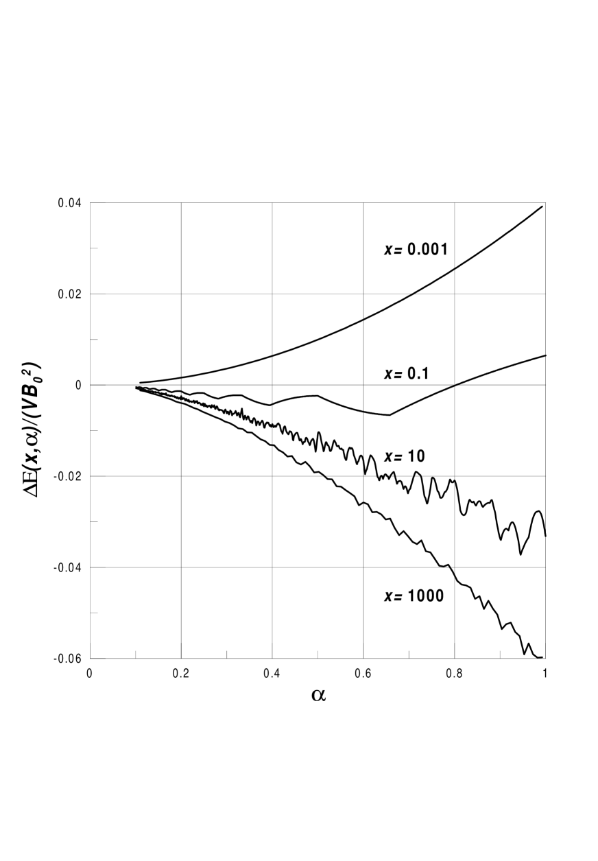
Figure 1: Total change of the dimensionless energy of the whole system as a function of the dimensionless chromomagnetic field $\alpha$.

In Fig. 2, the dimensionless energy gains in color ferromagnetic (with an optimal value of $\alpha$ is chosen) and superconducting phases are depicted as functions of the chemical potential $\mu$. The choice of the phase by the system is determined by the condition that the energy should take its minimum value in this phase.

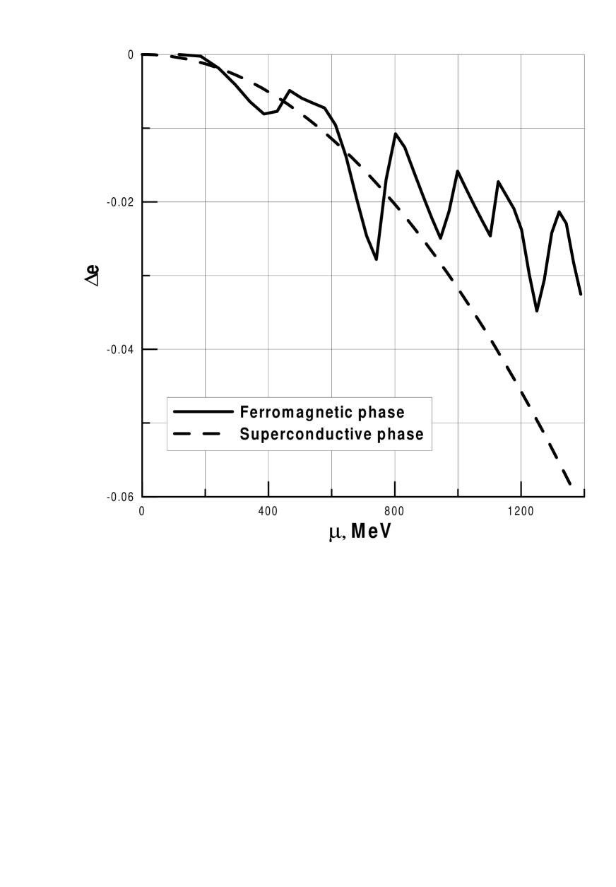
Figure 2: Dimensionless energy gain in a ferromagnetic phase (after a choice of an optimal value of $\alpha$ has been done) and in a superconducting phase as a function of the chemical potential $\mu$.

The consideration of the phase transition in the system leads to the conclusion that with large enough values of $\mu$, the superconducting phase is preferable. With lowering $\mu$, the ferromagnetic phase can become more preferable, and a phase transition takes place. However, one may see in the Figure that the energy gain corresponding to the ferromagnetic phase is an oscillating function of $\mu$, and hence the picture of phase transitions is somewhat more complicated. With further decrease of $\mu$, the superconducting phase may return, then again the ferromagnetic phase occurs, and this may repeat several times.

IV Phase transition at finite temperature

To describe the system at finite temperature, we should use the formulas for the termodynamic potential of fermions $\Omega_{q}(\alpha,\mu,T,B_{0})$, presented in Section 2. Restricting our consideration only to the main contribution of the ”classical ” chromomagnetic field $B^{2}/(8\pi)$, and neglecting small quantum fluctuations of the gluon field around it, we consider the contribution of fermions, defined by (17), (18), where we have to put $\Delta=0$, and hence use the formula

$$\Omega_{q}\,=\,-T\sum\limits_{k,i}\mbox{ln}\left[1+\mbox{exp}(\frac{\mu-\varepsilon_{k,i}}{T})\right].$$ (29)

It should be mentioned that unlike the case of zero temperature, at finite temperature the chemical potential $\mu$ becomes an independent variable and is no more equal to the Fermi energy.

As it was done in the case of zero temperature, we employ dimensionless variables and quantities, and moreover define a dimensionless temperature

$$\tau=\frac{T}{\sqrt{gB_{0}}}.$$ (30)

Since $\sqrt{gB_{0}}\sim 10^{2}$ MeV, we have for the temperature $T\sim 10^{8}$ eV $\sim 10^{12}K$.

Now in the case of finite temperature, we also use a numerical calculation method, which gives only approximate results, as we have to deal with an infinite series over the fermion energy levels. The results are shown in Figs. 3 and 4.

In Fig. 3, the dimensionless ferromagnetic gain of the total thermodynamic potential, minimized with respect to the dimensionless chromomagnetic field $\alpha=B/B_{0}$, is depicted:

$$\Delta\omega(\mu,\tau)\,=\,\mbox{min}_{\alpha}\left[\frac{\alpha^{2}}{8\pi}\,+\,\frac{1}{B_{0}^{2}}(\Omega_{q}(\alpha,\mu,T,B_{0})-\Omega_{q}(0,\mu,T,B_{0}))\right].$$ (31)

Our calculations demonstrate that, with growing temperature, oscillations in the plot of $\omega$ as a function of $\mu$ become less evident and, as it is seen in the Figure, in the limit of high temperature, they practically disappear. Another interesting observation is that even at zero chemical potential the appearance of a finite chromomagnetic field is preferable. This is due to the fact that at nonvanishing temperature, fermions exist with finite density even at $\mu=0$, and the appearance of a chromomagnetic field leads to a finite energy gain.

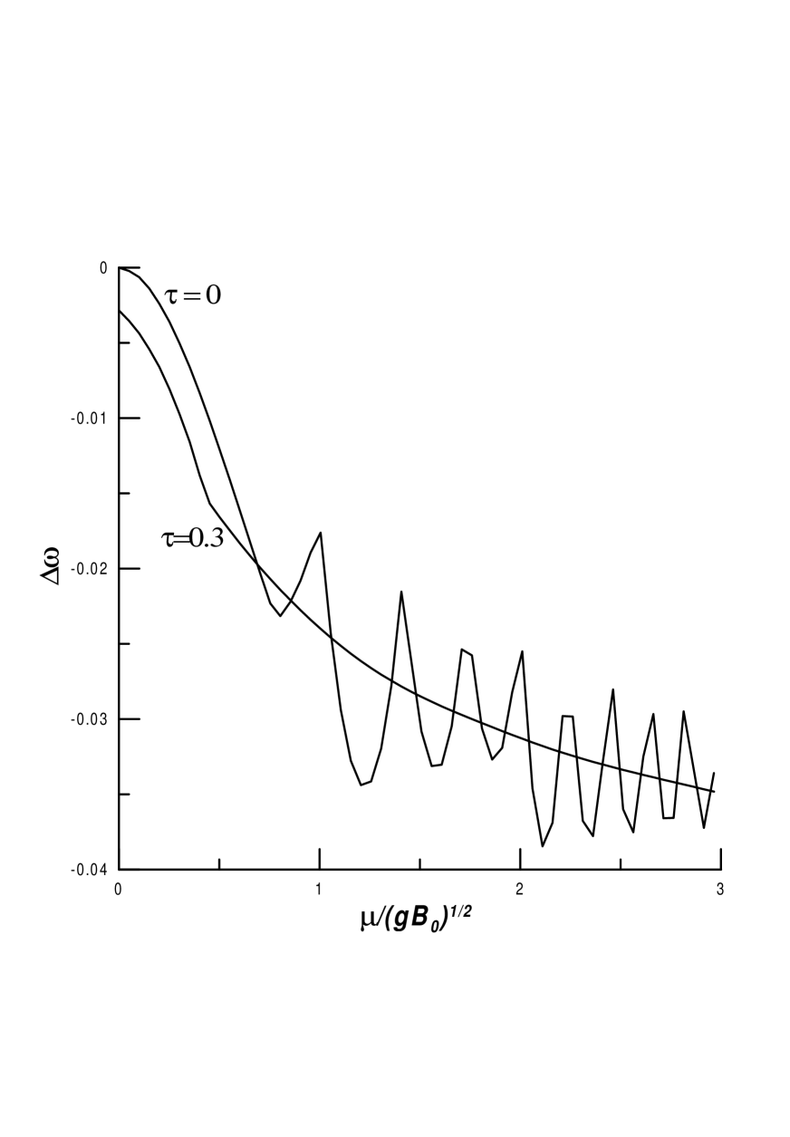
Figure 3: Dimensionless thermodynamic potential gain $\Delta\omega$ as a function of $\mu$ at zero and finite (sufficiently high) temperatures. The quantity $\tau$ is given by equation (30).

Figure 4 shows that with growing temperature and at fixed $\mu$, the thermodynamic potential gain $\Delta\omega$ tends to a constant value. It is seen that the higher the chemical potential, the lower temperature $\tau(\mu)$ is needed for stabilization of $\Delta\omega$ to take place. At low values of the chemical potential, $\Delta\omega$ decreases with growing temperature and it is stabilized at high enough temperature. These facts can be explained in the following way. The discrete character of the Landau levels is responsible for the nonmonotonic behavior of $\Delta\omega(\mu)$. This situation does not change while the temperature remains considerably lower than the distance between levels in the vicinity of the Fermi surface. It is clear that with growing $\mu$, the energy levels become distributed with greater density and hence, lower temperature is needed in order to smooth away oscillations.

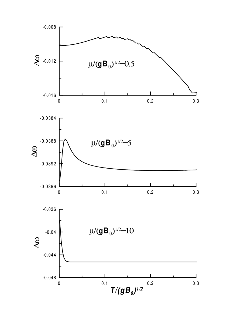
Figure 4: Stabilization of the thermodynamic potential gain with growing $T$ at various values of $\mu$.

V Conclusions

In the present paper we investigated further the gauge field model with a constant chromomagnetic field, i.e., the ferromagnetic state. We demonstrated that the method, proposed in iwaz1 , of finding a stabilized solution for this configuration, is valid only if a physically justified condition is fulfilled, i.e., the chromomagnetic field exists inside certain domains with finite dimensions. This implies that there is a maximum value of the chromomagnetic field inside the domain determined by the finite spatial extentnion of the region occupied by the field in the direction of the field.

The main object of our paper was to study the fermion sector of the model, and in particular to consider transitions between a color superconducting phase and a possible ferromagnetic phase from the point of view of comparing the energy gain in these phases. Our observations can be summarized as follows. At comparatively low densities of the baryon matter, quarks are confined, and exist only in colorless combinations. With growing chemical potential baryons approach each other to such close distancies that quarks become free particles. At sufficiently high density, the color superconducting phase can be formed. However, for ”intermediate ” values of the chemical potential, a ferromagnetic phase may emerge. There can be a phase transition between these two phases depending on which phase has larger energy gain. At zero or comparatively low temperatures a nontrivial phase structure can be formed, and this is due to a nonmonotonic dependence of the energy gain of fermions in the chromomagnetic field on their density. With growing chemical potential, a ferromagnetic state can prove to be favorable, then it is changed by a superconducting state, and then again ferromagnetic, and only for high enough chemical potentials, the superconducting state becomes always dominating.

At sufficiently high temperatures ($\sim\sqrt{gB_{0}}$), the phase structure is simplified. The fermion energy gain is no more dependent on temperature and becomes a monotonic function of $\mu$. For low $\mu$ the ferromagnetic phase becomes more favorable, and for large enough $\mu$, the superconducting phase, there being only one transition point between them. In the temperature scale, stabilization occurs at $T>T(\mu)$, where $T(\mu)$ is the minimal temperature needed to smooth out oscillations of the thermodynamic potential $\Omega$ that appear due to the discrete character of the fermion spectrum in the chromomagnetic field. Theoretical reasoning and computer calculations demonstrate that the function $T(\mu)$ should be decreasing.

Further investigations will help to describe more clearly the mechanism of formation of the chromomagnetic domains and to consider the boundary conditions in a more sophisticated manner. Moreover, in order to produce a more realistic picture of the process of the ferromagnetic phase formation, quantum fluctuations around the ”true vacuum ” state should be taken into account. Estimates showed that at a chemical potential sufficiently high for the ferromagnetic state to be formed, interactions between quarks are in no way week and should also be considered for. Certain changes to the picture of the process may further be given by the interaction of quarks with the charged boson condensate, and this should also be considered. Finally, one should also understand that in the case of the $SU(3)_{c}$ gauge group, there can be states with a color ferromagnetism in one $U(1)$ subgroup, and the color superconductivity in the other $U(1)$ subgroup of the maximal Abelian subgroup $U(1)\times U(1)$. These problems are to be considered in further investigations.

References

- (1) V.Ch. Zhukovsky, preprint Mad/TH/91-5 (1991), Univ. of Wisconsin-Madison; D. Ebert, V.Ch. Zhukovsky and A.S. Vshivtsev, Int. J. Mod. Phys. A13, 1723 (1998) .
- (2) A.V. Averin, A.V. Borisov and V.Ch. Zhukovsky, Z. Phys. C48, 457 (1990).
- (3) D. Ebert and V. N. Pervushin, Teor. Mat. Fiz. 36, 313 (1978); D. Ebert, Yu.L. Kalinovsky, L. Münchow and M.K. Volkov, Int. J. Mod. Phys. A8, 1295 (1993).
- (4) D. Ebert and H. Reinhardt, Nucl. Phys. B271, 188 (1986); D. Ebert, H. Reinhardt and M.K. Volkov, Progr. Part. Nucl. Phys. 33, 1 (1994).
- (5) A.S. Vshivtsev, V.Ch. Zhukovsky, K.G. Klimenko and B.V. Magnitsky, Phys. Part. Nucl. 29, 523 (1998).
- (6) K.G. Klimenko, Teor. Mat. Fiz. 89, 211 (1991); 90, 3 (1992); Z. Phys. C54, 323 (1992); I.V. Krive and S.A. Naftulin, Phys. Rev. D46, 2737 (1992); A.S. Vshivtsev, K.G. Klimenko and B.V. Magnitsky, JETP Lett. 62, 283 (1995); Teor. Mat. Fiz. 106, 319 (1996).
- (7) V.P. Gusynin, V.A. Miransky, and I.A. Shovkovy, Phys. Rev. Lett. 73, 3499 (1994).
- (8) V.P. Gusynin, Ukrainian J. Phys. 45, 603 (2000).
- (9) K.G. Klimenko, B.V. Magnitsky and A.S. Vshivtsev, Nuovo Cim. A107 (1994) 439; Theor. Math. Phys. 101, 1436 (1994); Phys. Atom. Nucl. 57, 2171 (1994).
- (10) D. Ebert and V.Ch. Zhukovsky, Mod. Phys. Lett. A12, 2567 (1997).
- (11) G.K. Savvidy, Phys. Lett., 71B, 133 (1977).
- (12) S.C.Matinyan, G.K.Savvidy, Nucl. Phys., B143, 539 (1978).
- (13) N.K. Nielsen and P. Olesen, Nucl. Phys. B 144, 376 (1978); B 160 380 (1979).
- (14) H.B.Nielsen and M. Ninomiya, Nucl. Phys. B 156, 1 (1979); ibid. B163, 57 (1980); ibid. B169 309 (1980); J. Ambjorn and P. Olesen, Nucl.Phys. B170 60, 265 (1980).
- (15) A. Cabo and A.E. Shabad, Trudy FIAN SSSR 111 (1979); A.Cabo, S.Penaranda and R.Martinez, Mod. Phys. Lett. A10 2413, (1995)
- (16) V. Skalozub, M. Bordag, Nucl. Phys., B576, 430 (2000).
- (17) V.V. Skalozub, A.V. Strelchenko, Eur. Phys. J., C33, 105 (2004).
- (18) A.O. Starinets, A.S. Vshivtsev, V.Ch. Zhukovsky, Phys. Lett., 322, 403 (1994)
- (19) S. C. Zhang, H. Hanson and S. Kivelson, Phys. Rev. Lett., 62, 82 (1989)
- (20) A. Iwazaki, O. Morimatsu, Phys. Lett., B571, 61 (2003); nucl-th/0304005.
- (21) A. Iwazaki, O. Morimatsu, T. Nishikawa, T. Ohtani, Phys. Lett., B579, 347 (2004); hep-ph/0309066; Phys. Rev., D47, 034014 (2005); hep-ph/0404201.
- (22) G. W. Semenoff, Phys. Rev. Lett. 61, 516 (1988).
- (23) M. Alford, K. Rajagopal and F. Wilczek, Phys. Lett. B422 247 (1998); Nucl. Phys. B537, 443 (1999)
- (24) K. Langfeld and M. Rho, Nucl. Phys. A660, 475 (1999); hep-ph/9811227.
- (25) J. Berges and K. Rajagopal, Nucl. Phys. B538, 215 (1999); hep-ph/9804233.
- (26) T.M. Schwarz, S.P. Klevansky and G. Papp, Phys. Rev., C60, 055205 (1999); nucl-th/9903048.
- (27) M. Alford, Ann. Rev. Nucl. Part. Sci. 51, 131 (2001); hep-ph/0102047.
- (28) M. Alford, Progr. Theor. Phys. Suppl., 153, 1 (2004); nucl-th/0312007.
- (29) I.A. Shovkovy, nucl-th/0410091.
- (30) D. Ebert, K.G. Klimenko and H. Toki, Phys. Rev. D64, 014038 (2001); hep-ph/0011273.
- (31) D.G. Yakovlev, A.D. Kaminker, P. Haensel, O.Y. Gnedin, Astron.&Astrophys., L24, 389 (2002).
- (32) F.M. Walter, J.M. Lattimer, Astrophys. J. L145, 576 (2002)
- (33) A.A. Sokolov, I.M.Ternov, V.Ch. Zhukovsky, and A.V. Borisov, Gauge Fields (in Russian), Moscow, 1986.
- (34) D. Ebert, V. V. Khudyakov, V. Ch. Zhukovsky, K.G. Klimenko, Phys. Rev., D65, 054024 (2002); hep-ph/0106110; V.Ch. Zhukovsky, K.G. Klimenko, V.V. Khudyakov and D.Ebert, JETP Lett. 74, 523 (2001).
- (35) K. Rajagopal, F. Wilczek, hep-ph/0011333.