Sneutrino warm inflation in the minimal supersymmetric model

Abstract

The model of RH neutrino fields coupled to the MSSM is shown to yield a large parameter regime of warm inflation. In the strong dissipative regime, it is shown that inflation, driven by a single sneutrino field, occurs with all field amplitudes below the Planck scale. Analysis is also made of leptogenesis, neutrino mass generation and gravitino constraints. A new warm inflation scenario is purposed in which one scalar field drives a period of warm inflation and a second field drives a subsequent phase of reheating. Such a model is able to reduce the final temperature after inflation, thus helping to mitigate gravitino constraints.

keywords: cosmology, inflation

I Introduction

In recent times, the idea of inflation being driven by the bosonic supersymmetric partner to a neutrino field has generated interest csnu ; hsnu . The idea is not new snuoriginal ; snusugra , but impetus has been gained after the experimental discovery of neutrino masses and mixing and an explanation through the seesaw mechanism seesaw . In supersymmetric realizations of the seesaw mechanism, the right-handed neutrinos have bosonic partners, sneutrinos, which are singlet fields, thus possible inflaton candidates. Model building typically proceeds by simply adding on the additional right-handed neutrino fields to an existing model. Thus the simplest supersymmetric model that emerges is an extended version of the MSSM, with now three families of right-handed neutrinos added on.

Two types of sneutrino inflation models have been examined, chaotic csnu and hybrid hsnu sneutrino inflation. The chaotic model is the simplest to construct, since all it requires is a monomial potential which can easily be obtained directly from the sneutrino fields. However this model suffers from the large field problem, in that the sneutrino field that drives inflation will have to have a field amplitude above the Planck scale. In the effective field theory interpretation of global Supersymmetric models, they are regarded as low-energy limits of some more complete supergravity (sugra) theory. However, for example in “minimal” sugra the exponential factor in front of the potential would prevent any scalar field from getting a value larger than $m_{P}$. Chaotic inflation would be possible with other more involved choices of the Khaler potential snusugra such that sugra corrections are kept under control. Still, in general in these models there are an infinite number of non-renormalizable operators suppressed by the Planck scale. As such, once the field amplitude exceeds this scale, an infinite number of parameters would require fine-tuning, so leaving no predictability in the theory. It is for this reason that chaotic inflation models are not amenable to particle physics model building. Hybrid inflation scenarios overcome the large field problem, since all field amplitudes are well below the Planck scale. However for sneutrino inflation, these models require introducing two additional superfields aside from the the right-handed neutrino fields hsnu . As such, this model is more contrived than the chaotic model. Nevertheless, up to now the hybrid model appears to be the simplest model in which to implement sneutrino inflation and be amenable to particle physics model building.

In this paper an even simpler model of sneutrino inflation is presented. In particular we show that monomial potentials, which can be constructed with only the right-handed sneutrino fields, when coupled to the MSSM, realize warm inflationary regimes. We show that in such regimes, due to the effect of strong dissipation, the field amplitudes of all sneutrino fields are well below the Planck scale, thus allowing such models to be consistent with particle physics model building.

The paper is organized as follows. The basic model is presented in Sect. II. The dissipative effects and basic equations of warm inflation for this model are obtained in Sect. III. The results of the sneutrino warm inflation scenario, which incorporates leptogenesis, are given in Sect. IV. A issue that emerges in Sect. IV is that the final temperature after inflation is too large to adequately control gravitino constraints. To improve this situation, in Sect. V a new warm inflation scenario is presented. In Sect VI neutrino mass generation from this scenario are examined. Finally in Sect. VII we summarize our results.

II Model

We consider the model of three generations of right-handed neutrinos, $N_{i}$, coupled to the MSSM with the superpotential

$$W=\frac{M_{i}}{2}N_{i}N_{i}+(h_{N})_{ij}H_{u}L_{i}N_{j}+(h_{L})_{ij}H_{d}L_{i}E^{c}_{j}+(h_{u})_{ij}H_{u}Q_{i}U^{c}_{j}+(h_{d})_{ij}H_{d}Q_{i}D^{c}_{j}\,.$$ (1)

The above model contains all the usual MSSM matter superfields, $H_{u}$, $H_{d}$ the Higgs doublets giving masses to the up and down quarks respectively, $Q_{i}$, the left-handed quarks, $U_{i}$, $D_{i}$, the right-handed up and down quarks respectively, and $L_{i}$, $E_{i}$ the left-handed and right-handed leptons. During inflation, assuming that at least one of the sneutrinos has got a non zero vacuum expectation value (vev), the relevant terms in the potential are:

$$V=M_{i}^{2}|N_{i}|^{2}+|(h_{N})_{ij}|^{2}|L_{i}H_{u}|^{2}+2Re[(h_{N}^{*})_{ij}M_{i}N_{j}L_{i}^{*}H_{u}^{*}]+|(h_{N})_{ij}|^{2}(|H_{u}|^{2}+|L_{i}|^{2})|N_{j}|^{2}+\cdots\,.$$ (2)

For a large value of $N_{i}$ we do not have to worry about soft susy breaking terms, and then all the spectrum remains massless ( $H_{u}=H_{d}=0$), except for the fields that couple directly to the sneutrinos, i.e., $H_{u}$ and the lepton doublets $L_{j}$. With $\langle N_{i}\rangle=\phi_{Ni}/\sqrt{2}$, the scalars for example get masses

$$m_{H_{u}}^{2}=\frac{1}{2}\sum_{j}h_{Nj}^{2}\phi_{Nj}^{2}\,$$ (3)

and similarly for the sleptons, where

$$h_{N_{j}}^{2}=\sum_{i}|(h_{N})_{ij}|^{2}\,.$$ (4)

III Dissipative inflationary dynamics

The interaction of the inflaton with other fields leads in general not only to modifications of the inflaton effective potential, but also to dissipative effects br05 ; br . These effects result in radiation production during inflation as well as modify the inflaton evolution equation with energy non-conserving terms. If these dissipative effects are adequately large, they can alter the standard picture of inflation, leading to warm inflation wi .

An analysis of various interaction configuration br05 ; br has shown that warm inflation occurs generically in many typical inflaton models. For example recently we showed in bb1 that the popular SUSY hybrid inflation model has a sizable parameter regime of warm inflation. In this section we show that warm inflation occurs in the sneutrino-MSSM model Eq. (1).

A basic interaction structure that has been shown in br05 ; br ; Hall:2004zr to produce sizable dissipative effects has the form of the bosonic inflaton field coupled to a heavy bosonic field which in turn is coupled to a light fermionic field. Such a structure can easily be identified in the sneutrino-MSSM model Eq. (1). For this consider the simplest case where only one sneutrino dominates the energy density during inflation, say $N_{1}$, thus acting the role of the inflaton field. Then from Eq. (1) the following relevant interaction configuration can be extracted

$${\cal L}_{I}=-|h_{N}|^{2}|N_{1}|^{2}|H_{u}|^{2}+h_{t}H_{u}\bar{t}_{R}t_{L}+h.c.,$$ (5)

thus the inflation $N_{1}$ couples to the up Higgs field, and for a large amplitude for $N_{1}$, the $H_{u}$ field then becomes heavy. This Higgs field in turn is coupled to the top fermion fields which are massless during inflation. Dissipative effects occur because as the inflaton amplitude changes, it implies a change to the $H_{u}$ mass. This results in a coherent excitation of the $H_{u}$ field, which then decays into the light top fermions with decay rate

$$\Gamma_{t}=\frac{3h_{t}^{2}}{16\pi}m_{H_{u}}\,.$$ (6)

From the dissipative calculations in Refs. br05 ; br this sort of interaction leads to the effective inflaton evolution equation

$$\ddot{\phi}+(3H+\Upsilon_{N})\dot{\phi}+V^{\prime}=0\,.$$ (7)

where the dissipative coefficient, based on the results in br05 ; br , can be determined to be

$$\Upsilon_{N}\simeq\frac{\sqrt{\pi}}{20}Y_{N}^{3/2}Y_{t}\phi_{N}\,,$$ (8)

with $Y_{N}\equiv h_{N}^{2}/(4\pi)$ and $Y_{t}={h_{t}^{2}}/{4\pi}$. Also in Eq. (7) the potential and the Hubble rate are

$$V\simeq\frac{1}{2}M_{N}^{2}\phi_{N}^{2}\$$ (9)

and

$$H^{2}\simeq\frac{M_{N}^{2}\phi_{N}^{2}}{6m_{P}^{2}}\,.$$ (10)

The dissipative term in Eq. (7) leads to radiation production which in the expanding spacetime obeys the equation

$$\dot{\rho}_{R}+4H\rho_{R}=\Upsilon_{N}\dot{\phi}_{S}^{2}\,.$$ (11)

Although the basic idea of interactions leading to dissipative effects during inflation is generally valid, the above set of equations has strictly been derived in br05 ; br only in the adiabatic-Markovian limit, i.e., when the fields involved are moving slowly, which requires

$$\frac{\dot{\phi}}{\phi}<H<\Gamma_{t}\,,$$ (12)

with $\Gamma_{t}$ being the decay rate Eq. (6). The second inequality, $H<\Gamma$ is also the condition for the radiation (decay products) to thermalize.

Thus in general any inflation model could have two very distinct types of inflationary dynamics, which have been termed cold and warm wi ; br05 ; br . The cold inflationary regime is synonymous with the standard inflation picture oldi ; ni ; ci , in which dissipative effects are completely ignored during the inflation period. On the other hand, in the warm inflationary regime dissipative effects play a significant role in the dynamics of the system. A rough quantitative measure that divides these two regimes is $\rho_{R}^{1/4}\approx H$, where $\rho_{R}^{1/4}>H$ is the warm inflation regime and $\rho_{R}^{1/4}\stackrel{{\scriptstyle<}}{{\sim}}H$ is the cold inflation regime. This criteria is independent of thermalization, but if such were to occur, one sees this criteria basically amounts to the warm inflation regime corresponding to when $T>H$. This is easy to understand since the typical inflaton mass during inflation is $m_{\phi}\approx H$ and so when $T>H$, thermal fluctuations of the inflaton field will become important. This criteria for entering the warm inflation regime turns out to require the dissipation of a very tiny fraction of the inflaton vacuum energy during inflation. For example, for inflation with vacuum (i.e. potential) energy at the GUT scale $\sim 10^{15-16}{\rm GeV}$, in order to produce radiation at the scale of the Hubble parameter, which is $\approx 10^{10-11}{\rm GeV}$, it just requires dissipating one part in $10^{20}$ of this vacuum energy density into radiation. Thus energetically not a very significant amount of radiation production is required to move into the warm inflation regime. In fact the levels are so small, and their eventual effects on density perturbations and inflaton evolution are so significant, that care must be taken to account for these effects in the analysis of any inflation models.

The conditions for slow-roll inflation ($\dot{\phi}_{S}^{2}\ll V$, $\ddot{\phi}_{S}\ll H\dot{\phi}_{S}$) are modified in the presence of the extra friction term $\Upsilon_{N}$, and we have now:

$$\epsilon_{\Upsilon} = \frac{\epsilon_{H}}{(1+r)^{2}}\simeq\frac{2}{C_{\Upsilon}^{2}}\left(\frac{M_{N}}{\phi_{N}}\right)^{2}\,,$$ (13)

$$\eta_{\Upsilon} = \frac{\eta_{H}}{(1+r)^{2}}\simeq\frac{2}{C_{\Upsilon}^{2}}\left(\frac{M_{N}}{\phi_{N}}\right)^{2}\,,$$ (14)

where

$$r\equiv\frac{\Upsilon_{N}}{3H}=\frac{\sqrt{6\pi}}{60}Y_{N}^{3/2}Y_{t}\frac{m_{P}}{M_{N}}=C_{\Upsilon}\frac{m_{P}}{M_{N}}\,.$$ (15)

and $\epsilon_{H}\equiv m_{P}^{2}V^{\prime 2}/(2V^{2})$, $\eta_{H}\equiv m_{P}^{2}V^{\prime\prime}/V$ are the standard cold inflation slow-roll parameters, in which there are no dissipation effects. In the slow-roll regime, when $\eta_{\Upsilon}<1$ and $\epsilon_{\Upsilon}<1$, Eqs. (7) and (11) are well approximated by:

$$\dot{\phi}_{S} \simeq -\frac{V^{\prime}}{3H}\frac{1}{1+r}\,,$$ (16)

$$\rho_{R} \simeq \frac{\Upsilon_{N}}{4H}\dot{\phi}_{S}^{2}\simeq\frac{1}{2}\frac{r}{(1+r)^{2}}\epsilon_{H}V\,,$$ (17)

and the number of e-folds is given by:

$$N_{e}\simeq-\int_{\phi_{Si}}^{\phi_{Se}}\frac{3H^{2}}{V^{\prime}}(1+r)d\phi\simeq\frac{(1+r)}{4m_{P}^{2}}\left(\phi_{Ne}^{2}-\phi_{end}^{2}\right)\,,$$ (18)

where $\phi_{Ne}(\phi_{end})$ is the value of the field at 60 e-folds (end of inflation). Inflation ends when $\epsilon_{\Upsilon}\simeq\eta_{\Upsilon}\simeq 1$ or when $\rho_{R}\simeq\rho_{N}$, whatever happens first. In the former case we have $\phi_{end}^{2}\simeq 2m_{P}^{2}/(1+r)^{2}$, whereas for $\rho_{R}\simeq\rho_{N}$ then $\phi_{end}^{2}\simeq m_{P}^{2}r/(1+r)^{2}$. In either case, taking $r\gg 1$, we get

$$\phi_{Ne}\simeq\sqrt{\frac{4N_{e}}{1+r}}m_{P}\,.$$ (19)

If we also want to keep the field below the Planck scale, we need $r>4N_{e}\simeq 240$. From Eq. (15), taking $|h_{N}|\simeq 1$, this gives the upper bound on the sneutrino mass $M_{N}\gtrsim 8\times 10^{12}$ GeV.

The effect of the dissipative term, in addition to producing a friction term for the inflaton field, leads to radiation production which can alter density perturbations. Approximately, one can say that when the radiation production leads to $T>H$, the fluctuations of the inflaton field are induced by the thermal fluctuations, instead of being vacuum fluctuations, with a spectrum proportional to the temperature of the thermal bath. We notice that having $T>H$ does not necessarily require $\Upsilon_{N}>3H$. Dissipation may not be strong enough to alter the dynamics of the background inflaton field, but it can be enough even in the weak regime to affect its fluctuations, and therefore the spectrum. Depending on the different regimes, the spectrum of the inflaton fluctuations $P^{1/2}_{\delta\phi}$ is given for cold inflation Guth:ec , weak dissipative warm inflation Moss:wn ; Berera:1995wh , and strong dissipative warm inflation Berera:1999ws respectively by

$$T<H: P^{1/2}_{\delta\phi}|_{T=0}\simeq\frac{H}{2\pi}\,,$$ (20)

$$\Upsilon_{N}<H<T: P^{1/2}_{\delta\phi}|_{T}\simeq\sqrt{TH}\sim\sqrt{\frac{T}{H}}P^{1/2}_{\delta\phi}|_{T=0}\,,$$ (21)

$$\Upsilon_{N}>H: P^{1/2}_{\delta\phi}|_{\Upsilon}\simeq\left(\frac{\pi\Upsilon_{N}}{4H}\right)^{1/4}\sqrt{TH}\sim\left(\frac{\pi\Upsilon_{N}}{4H}\right)^{1/4}\sqrt{\frac{T}{H}}P^{1/2}_{\delta\phi}|_{T=0}\,,$$ (22)

with the amplitude of the primordial spectrum of the curvature perturbation given by:

$$P^{1/2}_{\cal R}=\left|\frac{H}{\dot{\phi}_{S}}\right|P^{1/2}_{\delta\phi}\simeq\left|\frac{3H^{2}}{V^{\prime}}\right|(1+r)P^{1/2}_{\delta\phi}\,.$$ (23)

Given the different “thermal” origin of spectrum, the spectral index also changes with respect to the cold inflationary scenario arjunspectrum ; hmb1 ; warmspectrum ; warmrunning , even in the weak dissipative warm inflation regime when the evolution of the inflaton field is practically unchanged. General expressions for the spectral index are given in bb1 and those relevant to the model in this paper will be given in the sections that follow.

IV Sneutrino warm inflation

As we have seen, depending on the value of the dissipative coefficient $\Upsilon_{N}$, and therefore that of the ratio $r=\Upsilon_{N}/(3H)$, we can have standard cold inflation or warm inflation (with weak or strong dissipation). In sneutrino inflation with the minimal matter content of the MSSM plus 3 generations of RH (s)neutrinos as shown in Eq. (1), there is a well define dissipation channel during inflation due to the coupling of the RH sneutrinos to the Higgs $H_{u}$, and the coupling of $H_{u}$ to the top sector. From the experimental value of the top quark mass, $m_{t}=174(178)$ GeV mtop , the value of the top Yukawa coupling $h_{t}$ at the electroweak scale has to be close to one, with $m_{t}\simeq h_{t}(m_{t})v\sin\beta$, $v=\sqrt{v_{u}^{2}+v_{d}^{2}}=174$ GeV being the Higgs vacuum expectation value (vev), and $\tan\beta=\langle H_{u}\rangle/\langle H_{d}\rangle$ the ratio of the Higgs vevs. The top Yukawa coupling increases due to the running with the scale, and depending on the value of $\tan\beta$ it can reach the perturbative bound $h_{t}(M_{X})\simeq\sqrt{4\pi}$ at the unification scale $M_{X}$. Thus, although slightly model dependent, its value at the inflationary scale will be in the range $[1,\sqrt{4\pi}]$. Then, without lost of generality we can take its value close to the perturbative bound $Y_{t}=h_{t}^{2}/(4\pi)\simeq 1$, so that the dissipative coefficient Eq. (8) becomes $\Upsilon_{N}\approx\frac{\sqrt{\pi}}{20}Y_{N}^{3/2}\phi_{N}$. The free parameters in the model are then the sneutrino-inflaton mass $M_{N}$ and its Yukawa coupling $|h_{N}^{2}|$ defined in Eq. (4). Imposing the COBE normalization on the amplitude of the primordial spectrum of perturbations COBE ; WMAP generated during inflation, we can fix one of these parameters, say the mass $M_{N}$, as dependent on the value of the coupling $h_{N}$. This is plotted in Fig. (1), where we have included in addition to the value of $M_{N}$(GeV) the values of the dissipative ratio $r=\Upsilon_{N}/(3H)$, the field value in $m_{P}$ units at 60 e-folds, the temperature of the thermal bath at the end of inflation $T_{end}$, and the ratio $T/H$ during inflation. We can clearly distinguish the different regimes in the plot depending on the sneutrino Yukawa value. For very small values $|h_{N}|<10^{-3}$ we recover the standard cold inflation predictions, with $\phi_{N}>m_{P}$ and $M_{N}\simeq 2\times 10^{13}$ GeV. In this regime, the Yukawa coupling plays no role during inflation, and the normalization of the spectrum is set by the RH sneutrino mass, with $M_{N}\simeq 2\times 10^{13}$ GeV snuoriginal . The value of the Yukawa coupling fixes the decay rate of the sneutrino and therefore the final reheating $T$. In the simplest scenario where the inflaton is the lightest RH sneutrino, we would need $|h_{N}|<O(10^{-7}-10^{-6})$ if we want to keep $T_{RH}\leq 10^{7}-10^{8}$ GeV in order not to have problems with thermal production of gravitinos gravitinos . We remark that $T_{end}$ in fig. (1) is the temperature associated to the radiation energy density at the end of inflation due to dissipative effects, but this is not necessarily the reheating $T$ typically defined as the $T$ at which the inflaton completely decays and the Universe becomes radiation dominated. In the cold inflation scenario the radiation energy density at the end of inflation is always subdominant, and then reheating would proceed as usual by the subsequent decay of the sneutrino.

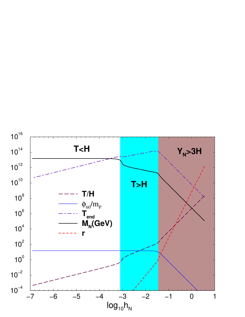
Figure 1: Values of the parameters $M_{N}$, $r$ and $\phi_{60}$ with respect to the sneutrino Yukawa coupling $|h_{N}|$, for cold inflation ($T<H$), weak dissipative regime ($T>H$, $\Upsilon_{N}<3H$), and strong dissipative regime ($T,\Upsilon_{N}/3>H$).

On the other hand, for a coupling $10^{-3}<|h_{N}|<10^{-1}$ inflation takes place in the weak dissipative regime, which would require a sneutrino mass of the order of $10^{12}-10^{11}$ GeV in order to fit the COBE amplitude of the spectrum. We notice that for these coupling and mass values, $|h_{N}|>10^{-3}$ and $M_{N}<10^{13}$ GeV, the adiabatic-Markovian approximation Eq. (12) holds. Still, the field values are larger than $m_{P}$. Again, the energy density in radiation is not dominant at the end of inflation, and $T_{end}$ is not necessarily the final $T_{RH}$. However, given that now we have a larger value of the coupling $|h_{N}|$, the standard estimation of $T_{RH}=(90/(\pi^{2}g_{*}))^{1/4}\sqrt{\Gamma_{N}m_{P}}$ in this regime would give a value $O(10^{12}\,GeV)$, beyond the gravitino constraint.

More interesting is the strong dissipative regime with $r>O(100)$ for $|h_{N}|\gtrsim 0.1$. In this regime field values are always kept below the cut-off scale $m_{P}$, which render the theory more attractive from the point of view of particle physics. The model can be considered as an effective model valid below the cut-off scale $m_{P}$, without the need of worrying about sugra corrections. Those are kept negligible for field values below Planck. The sneutrino mass value varies between $10^{10}$ GeV and $2\times 10^{5}$ GeV, decreasing with the value of the coupling. In particular, using Eqs. (22) and (23), the amplitude of the spectrum of primordial curvature perturbation is given by,

$$P_{\cal R}^{1/2}\simeq\frac{1}{2}\left(\frac{15}{64g_{*}}\right)^{1/8}(4N_{e})^{3/4}C_{\Upsilon}^{3/8}\left(\frac{M_{N}}{m_{P}}\right)^{3/8}\,,$$ (24)

and using $P_{\cal R}^{1/2}=5\times 10^{-5}$, (and $g_{*}=228.75$, the number of effective degrees of freedom for the MSSM) we have for $|h_{N}|\gtrsim 0.1$

$$|h_{N}|\simeq 8.2\times 10^{-2}\left(\frac{10^{10}GeV}{M_{N}}\right)^{1/3}.$$ (25)

This equation summarizes the constraint on the coupling and the sneutrino mass in order to have the strong dissipative regime. The larger the coupling $|h_{N}|$ is, the lighter the RH sneutrino.

In this regime inflation ends when the energy density in radiation becomes comparable to that of the sneutrino field and the Universe becomes radiation dominated. Therefore, in this case $T_{end}\simeq T_{RH}$, with values that are still larger than the gravitino bound. Another question is about leptogenesis in this scenario. One of the nice and more appealing features of sneutrino inflation is the possibility of relating in principle different pieces of physics like inflation, and neutrino masses and leptogenesis, through the physics of the RH neutrinos and their couplings. The lepton asymmetry $Y_{L}=n_{L}/s$ is generated by the out-of-equilibrium decay of the RH sneutrinos, and then reprocessed to the $B-L$ asymmetry by sphaleron processes at a temperature around $T\sim 100$ GeV, generating the observed baryon asymmetry $Y_{B}=n_{B}/s\simeq(8.7\pm 0.4)\times 10^{-11}$ WMAP . Successful thermal leptogenesis, with the initial RH sneutrino abundance produced out of the thermal bath, requires epsilonbound $T_{RH}\geq 2\times 10^{9}$ GeV, which is fulfilled for $|h_{N}|\lesssim 1.8$. It also requires a similar bound for the sneutrino mass, $M_{N}>2\times 10^{9}$ GeV, although the sneutrino dominating during inflation need not necessarily be the one originating the lepton asymmetry. We could have for example the lighter one with the larger Yukawa coupling as the inflaton, and the next-to-lightest being responsible for $Y_{L}$. Nevertheless, there are models where these bound can be evaded raidal .

Before closing this section, we comment on the predictions for the spectral index $n_{S}$, and the running of the spectral index $dn_{S}/d\ln k$, of the primordial spectrum. Those do not vary significantly from one regime to another. In the case of standard cold sneutrino inflation, we have $n_{S}-1\simeq-4/(2N_{e}+1)\simeq-0.03$ and $dn_{S}/d\ln k\simeq-32/(4N_{e}+2)^{2}\simeq-5\times 10^{-4}$, whereas in the strong dissipative regime we have $n_{S}-1\simeq-3/(2N_{e})\simeq-0.025$ and $dn_{S}/d\ln k\simeq-26/(4N_{e})^{2}\simeq-4.5\times 10^{-4}$. The distinctive prediction comes from the tensor-to-scalar ratio $r_{T}=P_{T}/P_{\cal R}$, with the primordial spectrum of the tensor modes being $P_{T}\simeq 2(H/2\pi m_{P})^{2}$. Whereas in cold sneutrino inflation, given that the field is larger than $m_{P}$, we have csnu ; snuoriginal $r_{T}\simeq 16\epsilon\simeq 0.16$, in the strong dissipative regime that ratio is highly suppressed, with

$$r_{T}\simeq 0.22\left(\frac{0.01}{|h_{N}|}\right)^{12}\,.$$ (26)

Future CMB experiment like Planck planck , and also gravitational wave detectors currently under study graviwaveback , are expected to reach a sensitivity for $r_{T}$ below 0.01. Therefore, the lack of a signal for the primordial spectrum of gravitational waves in future experiments will rule out sneutrino inflation in its more standard version, but not warm sneutrino inflation.

V Lowering the post-inflation temperature

Taking into account a lighter sneutrino from the very beginning, there is a simpler alternative that allows to lower the reheating $T$ at the end of warm inflation with strong dissipation, and which at the same time is compatible with generating the right level of baryon asymmetry by non-thermal leptogenesis. Let us denote by $\phi_{2}$, $M_{2}$ the field and mass parameter of the RH sneutrino dominating the energy density during inflation, and $\phi_{1}$, $M_{1}$ those of a lighter RH sneutrino. The dominant contribution during inflation is given by $\phi_{2}$, $V\simeq M_{2}^{2}\phi_{2}^{2}/2$, but still the lighter sneutrino can follow a slow-roll trajectory during inflation for field values below $m_{P}$, with the slow-roll parameter for $\phi_{1}$ being

$$\eta_{1} \simeq \frac{M_{1}^{2}}{M_{2}^{2}}\frac{2m_{P}^{2}}{\phi_{2}^{2}}\,,$$ (27)

$$\epsilon_{1} \simeq \eta_{1}\left(\frac{\phi_{1}}{\phi_{2}}\right)^{2}\,.$$ (28)

In order to have $\eta_{1}<1$, $\epsilon_{1}<1$, we only need to assume that the field values during inflation are comparable, $\phi_{1}\simeq\phi_{2}<m_{P}$, and require $M_{1}/M_{2}<(\phi_{2}/m_{P})_{end}\simeq 1/\sqrt{2r}$, which in terms of the coupling reads:

$$\frac{M_{1}}{M_{2}}\lesssim 1.6\times 10^{-5}|h_{N2}|^{-3}\,.$$ (29)

Having a second slow-rolling field does not change the primordial spectrum during or after inflation, so the estimation given in Eq. (24) applies, and the spectrum is dominated by thermal effects. Moreover, it does not matter what is the amplitude of the curvature perturbation generated by $\phi_{1}$ during inflation, by the end of inflation it has leveled to that of $\phi_{2}$. The constraint on the sneutrino mass dominating during inflation, $M_{2}\lesssim 10^{10}$ GeV, obtained in the previous section still applies.

During inflation the lightest sneutrino $\phi_{1}$ energy density is subdominant. When inflation ends for $\phi_{2}$ it does so for $\phi_{1}$. Then, this field, weakly coupled, starts oscillating and its energy density on average behaves like matter. Therefore, if its decay rate is small enough, it will end up dominating over the radiation energy density dissipated by $\phi_{2}$ during warm inflation. Later the field decays, and it is at this point that we define the final reheating $T$. Thus, the inflationary period is controlled by $\phi_{2}$, but the reheating phase is controlled by $\phi_{1}$, with

$$T_{RH}\simeq\left(\frac{90}{\pi^{2}g_{*}}\right)^{1/4}\sqrt{\Gamma_{1}m_{P}}\,,$$ (30)

where $\Gamma_{1}\simeq\frac{|h_{N1}|^{2}}{16\pi}M_{1}$, and then

$$|h_{N1}|\simeq 0.86\times 10^{-6}\times\left(\frac{T_{RH}}{10^{6}\,GeV}\right)\left(\frac{10^{8}\,GeV}{M_{1}}\right)\,.$$ (31)

Leptogenesis can now proceed through the out-of-equilibrium decay of the lightest sneutrino $\phi_{1}$ during the reheating period. Any previous lepton asymmetry would be diluted by the entropy produced by the $\phi_{1}$ decay. The lepton asymmetry at the end of reheating is then given by snuoriginal ; snusugra ,

$$\left.\frac{n_{L}}{s}\right|_{RH}\simeq|\epsilon_{1}|\frac{3T_{RH}}{4M_{1}}\,,$$ (32)

with $\epsilon_{1}$ being the CP asymmetry generated by the decay, given by the interference of the tree level with the one-loop amplitude,

$$|\epsilon_{1}|\simeq\frac{3}{8\pi(h_{N}^{\dagger}h_{N})_{11}}\sum_{i\neq 1}Im[(h_{N}^{\dagger}h_{N})_{1i}]^{2}\frac{M_{1}}{M_{i}}\,.$$ (33)

The asymmetry parameter is bounded by epsilonbound

$$|\epsilon_{1}|\leq\frac{3}{8\pi}\sqrt{\Delta m^{2}_{A}}\frac{M_{1}}{v_{u}^{2}}\simeq 2\times 10^{-8}\left(\frac{M_{1}}{10^{8}\,GeV}\right)\,,$$ (34)

where $\Delta m^{2}_{A}\simeq(1.3-4.2)\times 10^{-3}$ eV² is the the atmospheric neutrino mass squared difference atmospheric ; pdg . From Eqs. (32) and (34) we have then the bound csnu ; shafinL ,

$$\left.\frac{n_{L}}{s}\right|_{RH}\leq|\epsilon_{1}|\frac{3T_{RH}}{4M_{1}}\simeq 1.5\times 10^{-10}\frac{T_{RH}}{10^{6}\,GeV}\,,$$ (35)

and the baryon asymmetry:

$$\left.\frac{n_{B}}{s}\right|_{RH}\leq\frac{8}{23}\left.\frac{n_{L}}{s}\right|_{RH}\simeq 5\times 10^{-11}\frac{T_{RH}}{10^{6}\,GeV}\,,$$ (36)

and hence $T_{RH}\geq 2\times 10^{6}$ GeV in order to match the observed baryon asymmetry. On the other hand, in order to ensure the out-of-equilibrium decay of $\phi_{1}$ and avoid thermal washout of the asymmetry, we require $M_{N1}\geq T_{RH}$. Using Eqs. (25) and (29), the limiting value csnu $T_{RH}\simeq M_{N1}\simeq 10^{6}$ GeV is reached for $|h_{N2}|\lesssim 0.24$.

Therefore, we have a narrow window of values $0.1\lesssim|h_{N2}|\lesssim 0.24$, for which inflation happens in the strong dissipative regime with $M_{N2}\simeq 10^{10}-10^{9}$ GeV, but reheating with $T_{RH}\simeq 10^{6}$ GeV and non-thermal leptogenesis is given by the decay of a lighter sneutrino with parameters $5\times 10^{8}{\rm GeV}\gtrsim M_{N1}\gtrsim 10^{6}$ GeV and $2\times 10^{-7}\lesssim|h_{N1}|\lesssim 8.6\times 10^{-5}$. For having warm inflation with a larger Yukawa coupling $h_{N2}\gtrsim 0.24$, the second lighter and long-lived sneutrino with $M_{N1}<10^{6}$ GeV can lower the final reheating $T$ below the gravitino bound, but it does not seem consistent with non-thermal leptogenesis as we cannot satisfy at the same time $M_{N1}\gtrsim T_{RH}$ and $T_{RH}\simeq 10^{6}$ GeV. It would remain to check whether thermal leptogenesis could be viable during the reheating period in this case, for which one would need to set and study the Bolztman equations describing the evolution of the different number densities, which is beyond the scope of this paper.

VI Warm inflation and light neutrino masses

In this section we briefly want to comment on the issue of light neutrino masses with a not too heavy sneutrino $M_{N}\leq 10^{10}$ GeV but large Yukawa couplings $|h_{N}|\geq 0.1$. Over the recent years, different neutrino experiments have established the existence of neutrino oscillations driven by nonzero neutrino masses and neutrino mixing petkov . Atmospheric neutrino oscillation parameters read:

$$|\Delta m_{A}^{2}|=(1.3-4.2)\times 10^{-3}eV^{2}\,,\;\;\;\sqrt{|\Delta m_{A}^{2}|}\simeq 0.05eV\,,\;\;\;\sin 2\theta_{A}\geq 0.85\,,$$ (37)

while solar neutrino oscillation parameters lie in the low-LMA (large mixing angle) solution with:

$$|\Delta m_{sun}^{2}|=(8.5-7.4)\times 10^{-5}eV^{2}\,,\;\;\;\tan\theta_{sun}=0.4^{+0.09}_{-0.07}\,.$$ (38)

On the other hand, a combined analysis of the solar neutrino, CHOOZ and KamLAND data gives $\sin^{2}\theta_{13}<0.055$. An upper limit on the absolute value of the masses is obtained from WMAP data as $\sum_{j}m_{j}<(0.7-2.0)$ eV.

Given the superpotential Eq. (1), light neutrino masses are given by diagonalizing the see-saw mass matrix seesaw :

$$m_{LL}=v_{u}^{2}h_{N}M_{RR}^{-1}h_{N}^{T}=U_{\nu L}diag(m_{1},m_{2},m_{3})U_{\nu L}^{T}\,,$$ (39)

where $v_{u}=\langle H_{u}\rangle\sim 174$ GeV, $m_{i}$ the light LH neutrino masses, and $U_{\nu L}$ the rotation matrix. In the Yukawa matrix $h_{N}$, each column define a vector ${\bf h_{Ni}}$ with modulus $|h_{Ni}|$ as given in Eq. (4). In the eigenmass basis for the RH we have:

$$Tr\,m_{LL}=\sum_{i=1,2,3}m_{i}\simeq v_{u}^{2}\sum_{i=1,2,3}\frac{{\bf h_{Ni}\cdot h_{Ni}}}{M_{Ni}}<O(1){\rm eV}\,.$$ (40)

For the parameters of the strong dissipative regime we clearly exceed the WMAP bound, with ${\bf h_{N2}\cdot h_{N2}}/M_{N2}>O(30)$ eV.

However, this applies when assuming a diagonal mass matrix $M_{RR}$ in Eq. (39). We can work instead with inverted (see also raidal )

$$M_{RR}=\left(\begin{array}[]{ccc}0&M_{N2}&0\\ M_{N2}&0&0\\ 0&0&M_{N1}\end{array}\right)\,,$$ (41)

where

$$Tr\,m_{LL}=\sum_{i=1,2,3}m_{i}\simeq v_{u}^{2}\left(\frac{2{\bf h_{N3}\cdot h_{N2}}}{M_{N2}}+\frac{{\bf h_{N1}\cdot h_{N1}}}{M_{N1}}\right)<O(1){\rm eV}\,,$$ (42)

such that the large contribution coming from the large Yukawa coupling $h_{N2}$ can be canceled out by choosing an appropriate smaller coupling $h_{N3}\ll h_{N2}$. This kind of scheme gives rise to light neutrino masses with an inverted hierarchy, $m_{1}^{2}\approx m_{2}^{2}\gg m_{3}^{3}$. For example, taking ${\bf h_{N1}\cdot h_{N1}}/M_{N1}\ll{\bf h_{N3}\cdot h_{N2}}/M_{N2}$. We have then 2 almost degenerate light neutrino masses, with $|m_{1}|\simeq|m_{2}|\simeq\sqrt{|\Delta m_{A}^{2}|}$, and a massless one $m_{3}\simeq 0$, (small corrections from the Yukawas $h_{N1}$ gives a non-zero $m_{3}$ value). Atmospheric neutrino oscillations are given by oscillations among “13” and “23”, while solar data is explained by the oscillation between “12”, with $m_{1}^{2}-m_{2}^{2}\simeq\Delta m_{sun}^{2}$ inverted .

The mass parameter $M_{N1}$ can be larger or smaller than $M_{N2}$ as far as light neutrino masses are concerned. Nevertheless, if we choose the hierarchy $M_{N2}>M_{N1}$, the asymmetry parameter corresponding to the decay of the lightest sneutrino is given by:

$$|\epsilon_{Y}| \simeq \frac{3}{16\pi(|h_{N1}|^{2})}Im[({\bf h_{N3}^{*}\cdot h_{N1}})({\bf h_{N2}^{*}\cdot h_{N1}})]\frac{M_{N1}}{M_{N2}}$$ (43)

$$\simeq \frac{3}{8\pi}\sqrt{|\Delta m_{A}^{2}|}\frac{M_{N1}}{v_{2}^{2}}\,,$$

where in the second line we have just assumed that there is no hierarchy among the different components of ${\bf h_{N1}}$ and that phases are such that $Im[]$ is maximal and we saturate the upper bound on the asymmetry parameter.

VII Conclusion

The most important new feature for sneutrino inflation found in this paper is a model in which inflation is driven by just a single sneutrino field that creates a monomial inflationary potential, similar to chaotic sneutrino inflation snuoriginal ; snusugra ; csnu , but with the key difference that in the model of this paper the inflaton amplitude is below the Planck scale. For particle physics model building, this is an important feature, since this model is then not susceptible to large effects from higher dimensional operators. In particular, it can be embedded in a sugra potential even with minimal Kahler potential for the fields, with the exponential sugra correction in front of the potential remaining small and under control. The chaotic inflation scenario of the cold inflation picture has always been attractive for its simplicity, since it requires just a monomial potential to realize inflation. However the downside of this model for model building has been that the inflaton field amplitude necessary for inflation must be larger than the Planck scale, thus making the model highly susceptible to higher dimensional operator corrections. Now, taking into account dissipation, this simple model with a monomial potential can be regarded as an effective model truly valid below the cut-off scale $m_{P}$.

Before the results of this paper, the simplest sneutrino model that could maintain field amplitudes below the Planck scale was a version of hybrid inflation hsnu . But this model is more contrived since it requires additional fields aside from the RH neutrino fields. Thus the model of this paper is the simplest realistic realization of sneutrino inflation, in the sense that it is the minimal SUSY extension of the Standard Model to incorporate supersymmetry and RH neutrinos, it requires no additional fields beyond these to realize inflation, and all higher dimensional operators which inevitably also exist are all suppressed.

The key feature of our model that allowed the inflaton amplitude below the Planck scale with a monomial inflation potential was the presence of large dissipation in the inflaton evolution equation. Moreover as shown in Sect. III, the origin of these dissipative effects arise automatically at a first principles level for this model of RH neutrinos coupled to the MSSM. Thus we believe the model in this paper has several attractive features for building a complete model that is able to describe both particle physics and cosmology.

- (1) J. R. Ellis, M. Raidal, and T. Yanagida, Phys. Lett. B 581, 9 (2004)
- (2) S. Antusch, M. Bastero-Gil, S. F. King, and Q. Shafi, Phys. Rev. D71, 083519 (2005).
- (3) H. Murayama, H. Suzuki, T. Yanagida, and J. Yokoyama, Phys. Rev. Lett. 70, 1912 (1993).
- (4) H. Murayama, H. Suzuki, T. Yanagida, and J. Yokoyama, Phys. Rev. D50, 2356 (1994).
- (5) For a review see for example: S. King, Rep. Prog. Phys. 67, 107 (2004), and references therein.
- (6) A. Berera and R. O. Ramos, Phys. Rev. D 71, 023513 (2005); Phys. Lett. B 607, 1 (2005).
- (7) A. Berera and R. O. Ramos, Phys. Rev. D63 (2001) 103509; Phys. Lett. B567 (2003) 294.
- (8) A. Berera, Phys. Rev. Lett. 75 (1995) 3218; Phys. Rev. D54 (1996) 2519; Phys. Rev. D55 (1997) 3346.
- (9) M. Bastero-Gil and A. Berera, Phys. Rev. D 71, 063515 (2005).
- (10) P. Azzi et al., hep-ex/0404010; J. F. Arguin et al., hep-ex/0507006.
- (11) L. M. H. Hall and I. G. Moss, Phys. Rev. D 71, 023514 (2005).
- (12) A. H. Guth, Phys. Rev D23 (1981) 347; K. Sato, Phys. Lett. B99 (1981) 66.
- (13) A. Albrecht and P. J. Steinhardt, Phys. Rev. Lett. 48 (1982) 1220; A. Linde, Phys. Lett. 108B (1982) 389.
- (14) A. Linde, Phys. Lett. 129B (1983) 177.
- (15) A. H. Guth and S. Y. Pi, Phys. Rev. Lett. 49 (1982) 1110.
- (16) I. G. Moss, Phys. Lett. B 154, (1985) 120.
- (17) A. Berera and L. Z. Fang, Phys. Rev. Lett. 74 (1995) 1912.
- (18) A. Berera, Nucl. Phys. B 585, (2000) 666.
- (19) A. N. Taylor and A. Berera, Phys. Rev. D62 (2000) 083517.
- (20) L. M. H. Hall, I. G. Moss and A. Berera, Phys. Rev. D69 (2004) 083525.
- (21) W. Lee and L.-Z. Fang, Phys. Rev. D59 (1999) 083503; H. P. de Oliveira and S. E. Joras, Phys. Rev. D64 (2001) 063613; J. chan Hwang and H. Noh, Class. Quantum Grav. 19 (2002) 527
- (22) L. M. H. Hall, I. G. Moss and A. Berera, Phys. Lett. B589 (2004) 1.
- (23) G. F. Smoot et al., Astrophys. J. Lett. 396 (1996) L1; C. L. Bennet et al., Astrophys. J. Lett. 464 (1996) 1.
- (24) WMAP collab.: D. N. Spergel et al., astro-ph/0302209; G. Hinshaw et al., astro-ph/0302217; H. V. Peiris et al., astro-ph/0302225.
- (25) M. Y. Khlopov and A. D. Linde, Phys. Lett. B138 (1984), 265–268; J. R. Ellis, J. E. Kim, and D. V. Nanopoulos, Phys. Lett. B145 (1984), 181; J. R. Ellis, D. V. Nanopoulos, and S. Sarkar, Nucl. Phys. B259 (1985), 175; T. Moroi, H. Murayama, and M. Yamaguchi, Phys. Lett. B303 (1993), 289–294; M. Kawasaki, K. Kohri, and T. Moroi, astro-ph/0402490.
- (26) M. Bolz, A. Branderburg, W. Buchüller, Nucl. Phys. B606 (2001) 518. gravitinos
- (27) For a review on gauge mediation models, see for example: G. F. Giudice and R. Rattazzi, Phys. Rept. 322 (1999) 419.
- (28) M. Fuji and T. Yanagida, Phys. Lett. B 549 (2002) 273; M. Fuji, M. Ibe and T. Yanagida, Phys. Rev. D69 (2004) 015006.
- (29) T. Gherghetta, G. F. Giudice and J. D. Wells, Nucl. Phys. B559 (1999) 27.
- (30) K. Hamaguchi, H. Murayama, and T. Yanagida, Phys. Rev. D65 (2002), 043512, hep-ph/0109030; S. Davidson and A. Ibarra, Phys. Lett. B535 (2002), 25–32, hep-ph/0202239; G. F. Giudice, A. Notari, M. Raidal, A. Riotto, A. Strumia, Nucl. Phys. 685 (2004) 89.
- (31) M. Raidal, A. Strumia and K. Turzyński, hep-ph/0408015.
- (32) http://www.rssd.esa.int/index.php?project=PLANCK
- (33) T. L. Smith, M. Kamionkowski and A. Cooray, astro-ph/0506422.
- (34) Y. Fukuda et al., Phys. Rev. Lett. 81 (1998) 1562; Y. Ashie et al., Phys. Rev. Lett. 93 (2004) 101801.
- (35) “Review of Particle Physics”, S. Edidelman et al., Phys. Lett. B592 (2004) 1.
- (36) T. Asaka, K. Hamaguchi, M. Kawasaki, T. Yanagida, Phys. Lett. B464 (1999) 12; V. N. Senoguz and Q. Shafi, Phys. Lett. B582 (2004) 6; V. N. Senoguz and Q. Shafi, Phys. Rev. D71 (2005) 043514.
- (37) See for example: S. T. Petkov, hep-ph/0504166
- (38) R. Barbieri, L. Hall, D. Smith, A. Strumia and N. Weiner, JHEP 9812 (1998) 17; A. S. Joshipura, S. D. Rindani, Eur. Phys. J. C14 (2000) 85; R. N. Mohapatra, A. Perez-Lorenzana and C. A. de S. Pires, Phys. Lett. B474 (2000) 355; S. F. King and N. Nimai Singh, hep-ph/0007243.