Single–Spin Asymmetries in the Bethe–Heitler Process $e^{-}+p\rightarrow e^{-}+\gamma+p$
from QED Radiative Corrections

Abstract

We derived analytic formulae for the polarization single–spin asymmetries (SSA) in the Bethe–Heitler process $e^{-}+p\rightarrow e^{-}+\gamma+p$. The asymmetries arise due to one-loop QED radiative corrections to the leptonic part of the interaction and present a systematic correction for the studies of virtual Compton Scattering on a proton through interference with the Bethe-Heitler amplitude. Considered are SSA with either longitudinally polarized electron beam or a polarized proton target. The computed effect appears to be small, not exceeding 0.1 per cent for kinematics of current virtual Compton scattering experiments.

I Introduction

Experiments on virtual Compton scattering (VCS) and deeply-virtual Compton scattering (DVCS) are an important part of nucleon structure studies at major electron-scattering laboratories, and at Jefferson Lab in particular JLab12GeV . The reason for such a high interest is that VCS allows to access 3-dimensional parton distributions of a nucleon and has a potential of resolving the role of parton orbital angular momentum in the nucleon spin problem, see the original papers GPD and recent reviews Diehl:2003ny ; Belitsky:2005qn .

In experimental observations, the VCS amplitude of electroproduction of real photons competes with a large and often dominant Bethe-Heitler (BH) amplitude, in which the real photon is emitted by leptons in the scattering process. In the leading order in electromagnetic interactions, single-spin asymmetries (SSA) in electroproduction of real photons are caused only by the VCS amplitude, including its interference with BH process. BH amplitude alone does not lead to SSA, unless higher-order electromagnetic corrections are included. Here we present a calculation of SSA coming from such corrections.

The fact that QED loop radiative corrections can induce the beam SSA in $\gamma-p$ and $e^{-}-p$ collisions with production of a $e^{+}e^{-}$-pair or radiation of a photon is known for a long time. A spin-momentum correlation in differential cross sections for these processes were first considered by Olsen and Maximon in 1959 OM , and somewhat later in other publications Oth . It was shown that a large azimuthal asymmetry originates from interference of the first and second (two–photon exchange) Born approximation. These studies addressed primarily the case of low energies, such that $\omega/M<<1$, where $\omega$ is the energy of the incoming polarized particle and $M$ is the target mass.

More recently it was pointed out, for example, in Ref.AKMP that SSA can be induced also by a pure loop correction to the lepton part of the interaction. For the related processes of radiative Möller scattering and electron-positron pair production on an electron target, the calculation of Ref.AKMP yields substantial SSA, reaching tens of per cent in selected kinematics. Asymmetries of this magnitude could present a significant systematic correction to VCS studies, and this fact partly motivated our present calculation spanning a broad kinematic range. In Ref.Mark the corresponding effect is included in the full radiative correction to beam SSA due to interference between BH and (the absorptive part of) nucleon VCS amplitudes. In Ref.Mark the full correction to the beam SSA was computed numerically, but up to now there is no published analytic expressions for the beam SSA caused by the loop correction to the leptonic tensor, that is simple enough to include in Monte Carlo generators for analysis of VCS experiments. The present paper aims at closing this gap. In addition, using an unpolarized leptonic Compton tensor originally derived in Ref.KMF , we obtain new results for SSA in the BH process with a polarized proton target arising from QED loop corrections.

The QED effects considered in this paper are referred to as model-independent, since they do not require additional knowledge of the nucleon structure. They represent systematic corrections to SSA measurements such as CLAS1 ; HERMES ; CLAS2 ; HallA ; d'Hose:2002us in the interference region between BH and VCS amplitudes of electroproduction of real photons.

II General Formalism and Beam Single-Spin Asymmetry

The contribution to the beam SSA for the BH process,

$$e^{-}(k_{1})+P(p_{1})\rightarrow e^{-}(k_{2})+\gamma(k)+P(p_{2}),$$ (1)

induced by one–loop corrections to the leptonic part of interaction in the case of longitudinally polarized incoming electrons can be written in terms of contraction of the leptonic and hadronic tensors

$$A^{b}=\frac{\alpha}{4\pi}\frac{\Re e[P^{(1)}_{\mu\nu}H_{\mu\nu}]}{B_{\mu\nu}H_{\mu\nu}}\ ,$$ (2)

where the symbol $\Re e$ denotes the real part and $B_{\mu\nu}$ is an unpolarized leptonic tensor for large-angle photon emission in the process (1). We define it as

$$B_{\mu\nu} = \frac{1}{4}Tr(\hat{k}_{2}+m)O_{\lambda\mu}(\hat{k}_{1}+m)O_{\nu\lambda}\ ,$$ (3)

$$O_{\lambda\mu} = \gamma_{\lambda}\frac{\hat{k}_{2}+\hat{k}+m}{s}\gamma_{\mu}+\gamma_{\mu}\frac{\hat{k}_{1}-\hat{k}+m}{t}\gamma_{\lambda}\ ,s=2kk_{2},\ t=-2kk_{1}\ ,$$

where $m$ is the electron mass. Note that both Mandelstam invariants ($s$ and $t$) in experiments that study proton VCS CLAS1 ; HERMES ; HallA ; CLAS2 ; d'Hose:2002us are large, therefore in our calculations we can omit the lepton mass in the quantity $B_{\mu\nu}$ and write the latter in the form

$$B_{\mu\nu}=\frac{(s+u)^{2}+(t+u)^{2}}{st}\tilde{g}_{\mu\nu}+\frac{4\Delta^{2}}{st}(\tilde{k}_{1\mu}\tilde{k}_{1\nu}+\tilde{k}_{2\mu}\tilde{k}_{2\nu})\ ,\\ u=-2k_{1}k_{2}\ ,\ \Delta=k_{2}-k_{1}+k=p_{1}-p_{2},\ \Delta^{2}=s+t+u,$$ (4)

where the tilde notation for 4-vectors denotes the gauge-invariant substitution, $\tilde{a}_{\mu}=a_{\mu}-\Delta_{\mu}\frac{a\Delta}{\Delta^{2}}$.

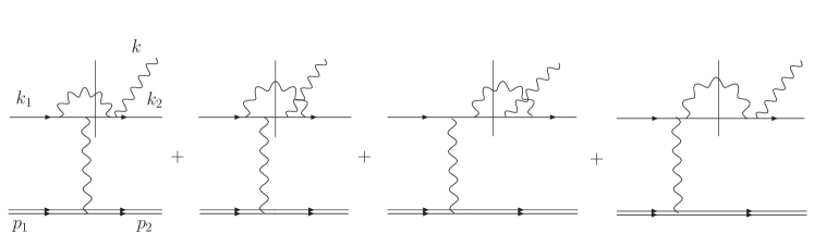
Figure 1: One-loop corrected diagrams that induce single-spin asymmetries in the BH process (1). Only radiation from the outgoing electron contributes. Vertical solid lines indicate the unitarity cuts.

For the hadronic tensor, we use its Born expression

$$H_{\mu\nu}=\frac{1}{4}Tr(\hat{p}_{2}+M)\Gamma_{\mu}(\hat{p}_{1}+M)(1-\gamma_{5}\hat{S})\Gamma_{\nu}\ ,\ \Gamma_{\mu}=(F_{1}+F_{2})\gamma_{\mu}-\frac{p_{1\mu}+p_{2\mu}}{2M}F_{2}\ ,$$

where $F_{1,2}\equiv F_{1,2}(\Delta^{2})$ are the Dirac and Pauli proton form factors, respectively, and $S$ is a 4–vector of proton polarization. The expressions for spin–independent and spin–dependent parts of the hadronic tensor are

$$H^{(un)}_{\mu\nu}=\frac{\Delta^{2}}{2}\big{(}F_{1}+F_{2})^{2}\tilde{g}_{\mu\nu}+2\Big{(}F_{1}^{2}-\frac{\Delta^{2}}{4M^{2}}F_{2}^{2}\Big{)}\tilde{p}_{1\mu}\tilde{p}_{1\nu}\ ,$$ (5)

$$H^{S}_{\mu\nu}=-iM(F_{1}+F_{2})(\mu\nu\Delta\rho)\Big{[}\Big{(}F_{1}+\frac{\Delta^{2}}{4M^{2}}F_{2}\Big{)}S_{\rho}+\frac{F_{2}(Sp_{2})}{2M^{2}}p_{1\rho}\Big{]}\ ,$$ (6)

where $(\mu\nu\Delta\rho)\equiv\epsilon_{\mu\nu\lambda\rho}\Delta_{\lambda}$ and the sign convention for the Levi-Civita tensor is $\epsilon_{0123}=1.$ Only the spin-independent hadronic tensor contributes to the beam SSA, therefore contraction of the tensors reads

$$H^{(un)}_{\mu\nu}B_{\mu\nu} = \frac{(s+u)^{2}+(u+t)^{2}}{st}\Big{[}\Delta^{2}(F_{1}+F_{2})^{2}+2M^{2}\Big{(}F_{1}^{2}-\frac{\Delta^{2}}{4M^{2}}F_{2}^{2}\Big{)}\Big{]}+$$ (7)

$$\frac{2\Delta^{2}}{st}\Big{(}F_{1}^{2}-\frac{\Delta^{2}}{4M^{2}}F_{2}^{2}\Big{)}\big{[}V^{2}+X^{2}+V(u+t)-X(u+s)\big{]}\ ,$$

where $V=2k_{1}p_{1},\ X=2k_{2}p_{1}$.

Let us now consider the leptonic tensor. In general, its spin-dependent part for the case of the beam longitudinal polarization can be written as

$$P_{\mu\nu}=P^{(0)}_{\mu\nu}+\frac{\alpha}{4\pi}P^{(1)}_{\mu\nu}\ ,$$ (8)

where the Born value $P^{(0)}_{\mu\nu}$ is pure imaginary and antisymmetric and therefore it does not contribute in the beam SSA, whereas the one-loop correction to it $P^{(1)}_{\mu\nu}$, together with the imaginary antisymmetric part, contains also the the real and symmetric part. The latter is caused by interference between the Born-level BH amplitude and the diagrams in Fig.1 with an additional photon loop and an external photon coupling to the outgoing electron. These diagrams produce a nonzero imaginary (absorptive) part of the amplitude in the physical region of the process (1) due to two-particle electron-photon intermediate states as shown in Fig.1 by the unitarity cuts.

Calculation of the one-loop diagrams of Fig.1 contributing to the radiative leptonic tensor can be done by standard QED techniques. Details of the calculation can be found in Ref.KMF for unpolarized electrons and in Ref.AAK for longitudinally polarized electrons. In calculations of SSA, we are only concerned with the absorptive parts of the electron virtual Compton amplitude that enters the radiative leptonic tensor. It should be noted that calculation of SSA is infra-red safe, i.e., infra-red singularities explicitly cancel at the loop level for this observable. It is an important consistency check of the calculation, since ultra-soft photon radiation that normally cancels such singularities has zero absorptive part and therefore cannot assist with infra-red divergence cancellation in the considered observable.

The contribution to $P^{(1)}_{\mu\nu}$ we are interested in can be derived by standard loop computation techniques of QED. Neglecting terms that are explicitly anti-symmetric in indices $\mu\leftrightarrow\nu$, we arrive at the following expression ($c.f.$ Eq.(36) of Ref.AAK ),

$$P^{(1)}_{\mu\nu}=i(k_{1}k_{2}\Delta\nu)[B_{1}\tilde{k}_{1\mu}+B_{2}\tilde{k}_{2\mu}]-i(k_{1}k_{2}\Delta\mu)[B^{*}_{1}\tilde{k}_{1\nu}+B^{*}_{2}\tilde{k}_{2\nu}]\ ,$$ (9)

where the quantity $B_{1}$ has the form

$$B_{1} = \frac{2}{st}\Big{[}\frac{8u}{a}\big{(}1-\frac{\Delta^{2}}{a}L_{\Delta u}\big{)}+\frac{6t}{b}L_{\Delta t}+\frac{2(u^{2}-2s^{2}-su)}{cu}L_{s\Delta}+$$

$$\frac{2b}{c}\big{(}1+\frac{s}{c}L_{s\Delta}\big{)}+\frac{2}{s}(2c-s)L_{tu}+\big{(}-2-\frac{4c^{2}}{st}-\frac{12b}{t}-\frac{4s^{2}}{ut}\big{)}L_{\Delta u}+\frac{4b^{2}}{ut}L_{su}+$$

$$\big{(}-2+\frac{2uc}{s^{2}}-\frac{2t}{s}\big{)}G+\big{(}\frac{2b}{t}+\frac{2b^{2}}{t^{2}}\big{)}\widetilde{G}+6\Big{]}\ ,$$

where, except for the 4-vector $\Delta$, we used the same notation as in AAK (see also KMF ),

$$(k_{1}k_{2}\Delta\sigma) = \epsilon_{\alpha\beta\lambda\sigma}k_{1\alpha}k_{2\beta}\Delta_{\lambda}\ ,\ a=s+t,\ b=s+u,\ c=t+u\ ,$$ (11)

$$G = L_{\Delta u}(L_{\Delta}+L_{u}-2L_{t})-\frac{\pi^{2}}{3}-2Li_{2}\big{(}1-\frac{\Delta^{2}}{u}\big{)}+2Li_{2}\big{(}1-\frac{t}{\Delta^{2}}\big{)}\ ,$$

$$L_{xy} = L_{x}-L_{y}\ ,\ \ L_{\Delta}=\ln\frac{-\Delta^{2}}{m^{2}}\ ,\ L_{u}=\ln\frac{-u}{m^{2}}\ ,\ L_{t}=\ln\frac{-t}{m^{2}}\ ,\ L_{s}=\ln\frac{-s}{m^{2}}\ .$$

The quantities $B_{2}$ and $\widetilde{G}$ can be derived from $B_{1}$ and $G$ by substitution

$$B_{2}=-B_{1}(s\leftrightarrow t),\ \ \widetilde{G}=G(s\leftrightarrow t)\ .$$

Imaginary parts of $B_{1}$ and $B_{2}$ which induce the real symmetric part of $P^{(1)}_{\mu\nu}$ can arise from the terms containing $L_{s}$ and $\widetilde{G},$ and the terms contributing to the imaginary part of $\widetilde{G}$ are $L_{s}$ and $Li_{2}(1-s/\Delta^{2})$ because of the condition $1-s/\Delta^{2}>1.$ From the form of proparators in the Feynman diagrams of Fig.1 it follows that to obtain the imaginary part of $B_{1}$ and $B_{2}$, one has to add a small negative imaginary part to the electron mass. It leads to

$$L_{s}=\ln\frac{s}{m^{2}}-i\pi,\ \ Li_{2}\big{(}1-\frac{s}{\Delta^{2}}\big{)}=-\int\limits_{0}^{1-s/\Delta^{2}}\frac{dx\ln{x}}{1-x}-\ln\frac{u+t}{\Delta^{2}}L_{s\Delta}\ ,$$ (12)

and it means that

$$\Im m\widetilde{G}=2\pi\ln\frac{u+t}{u}\ ,$$

where the symbol $\Im m$ stands for the imaginary part. By combining the previous results, we arrive at

$$\Im mB_{1} = -\frac{2\pi}{st}\bar{B_{1}}\ ,\ \ \Im mB_{2}=-\frac{2\pi}{st}\bar{B_{2}}\ ,$$

$$\bar{B}_{1} = \frac{2\Delta^{2}(\Delta^{2}-t)}{t}\bigl{[}\frac{3t+2u}{(t+u)^{2}}-\frac{2}{t}\ln(1+\frac{t}{u})\bigr{]},$$ (13)

$$\bar{B}_{2} = \frac{2\Delta^{2}}{t}\bigl{[}\frac{t-2u}{t+u}-2(1-\frac{u}{t})\ln(1+\frac{t}{u})\bigr{]}$$

Note that the terms containing anomalous poles at $t\rightarrow 0$ are cancelled explicitly in Eqs. (II). Moreover, both $\bar{B}_{1}$ and $\bar{B}_{2}$ are proportional to $t$ if $t\to 0$. Contraction of the tensors in the numerator of Eq.(2) can be written in the following form that appears as a factor in the spin-dependent numerator for beam SSA:

$$P^{(1)}_{\mu\nu}H_{\mu\nu}=\frac{2\pi(k_{1}k_{2}\Delta p_{1})}{st}\Big{(}F_{1}^{2}-\frac{\Delta^{2}}{4M^{2}}F_{2}^{2}\Big{)}[(2V-s+\Delta^{2})\bar{B}_{1}+(2X-s-u)\bar{B}_{2}]\ .$$ (14)

An important observation is that the expressions (II) contain an overall factor of $\Delta^{2}$, that is a squared 4-momentum transferred to the proton target. Since experiments on DVCS select small values of $\Delta^{2}$, it directly implies additional suppression of beam SSA in this region.

Equations (2),(7), (II-14) determine the beam SSA for the BH process (1). Note that the expressions for SSA do not contain large logarithms involving the lepton mass.

Let us now introduce kinematic invariants used to define experimentally measured asymmetries in VCS. The following set of kinematic variables Bal is accepted for experimental analyses: Azimuthal angle $\Phi$ between planes $({\bf q}_{1},{\bf k}_{1})$ and $({\bf q}_{1},{\bf p}_{2})$ in laboratory system (with axes $OZ$ along direction $-{\bf q}_{1}={\bf k}_{2}-{\bf k}_{1}),$ and invariant variables

$$x=\frac{-q_{1}^{2}}{2p_{1}q_{1}}\ ,\ \ y=\frac{2p_{1}q_{1}}{V}\ ,\ \ \ \ q_{1}=k_{1}-k_{2},\ q_{1}^{2}\equiv u.$$ (15)

The advantage of these variables is that one may use both the laboratory system and c.m.s. of subprocess $\gamma(q_{1})+P(p_{1})\rightarrow\gamma(k)+P(p_{2})$ to investigate the azimuth correlation. The reason is that c.m.s. can be reached from laboratory system by a boost along the direction of ${\bf q}_{1},$ and such transformation does not change the azimuthal angle $\Phi.$ Therefore, we can use the simple expressions for the particle energies and their angles in c.m.s.

$$p_{1} = (E_{1},0,0,|{\bf p}_{1}|),\ p_{2}=(E_{2},|{\bf p}_{2}|\sin{\theta_{N}}\cos{\Phi},|{\bf p}_{2}|\sin{\theta_{N}}\sin{\Phi},|{\bf p}_{2}|\cos{\theta_{N}}),$$ (16)

$$k_{1} = \varepsilon_{1}(1,\sin{\theta_{1}},0,\cos{\theta_{1}}),\ k_{2}=\varepsilon_{2}(1,\sin{\theta_{2}},0,\cos{\theta_{2}}),$$

$$k = (k_{0},-{\bf p}_{2}),\ \ q_{1}=(\varepsilon_{1}-\varepsilon_{2},-{\bf p}_{1})$$

in terms of variables (15) to form all the invariants that enter into beam and target asymmetries. They read

$$\varepsilon_{1} = \frac{V(1-xy)}{2\sqrt{\xi V}}\ ,\ \varepsilon_{2}=\frac{V(1-y+xy)}{2\sqrt{\xi V}}\ ,k_{0}=\frac{V(y-xy)}{2\sqrt{\xi V}}\ ,$$

$$E_{1} = \frac{V(y+2\tau)}{2\sqrt{\xi V}}\ ,\ E_{2}=\frac{V(y-xy+2\tau)}{2\sqrt{\xi V}}\ ,$$

$$\cos{\theta_{1}} = -\frac{y(1-2x+xy+2x\tau)}{\lambda(1-xy)}\ ,\ \cos{\theta_{2}}=-\frac{y(1-2x-y+xy-2x\tau)}{\lambda(1-y+xy)}\ ,$$ (17)

$$\sin{\theta_{1}} = \frac{2\sqrt{\eta\xi xy}}{\lambda(1-xy)}\ ,\ \ \sin{\theta_{2}}=\frac{2\sqrt{\eta\xi xy}}{\lambda(1-y+xy)}\ ,$$

$$\cos{\theta_{N}} = \frac{y(y-xy+2x\tau)-2\xi\rho}{\lambda(y-xy)}\ ,\ \ \sin{\theta_{N}}=\frac{2\xi\sqrt{\rho_{+}-\rho)(\rho-\rho_{-})}}{\lambda(y-xy)}\ ,$$

where we used the following brief notation

$$\lambda^{2} = y^{2}+4xy\tau,\ \ \eta=1-y-xy\tau,\ \ \xi=y-xy+\tau,\ \ \tau=\frac{M^{2}}{V}\ ,$$ (18)

$$\rho = \frac{-\Delta^{2}}{V},\ \ \rho_{\pm}=\frac{y}{2\xi}[(1-x)(y\pm\lambda)+2x\tau].$$

Here we introduced a dimensionless variable $\rho$ with the quantities $\rho_{\pm}$ having a meaning of the minimum $(\rho_{-})$ and maximum $(\rho_{+})$ value of $\rho$ at fixed $x,\ y$ and $V.$ By using relations (II) it is straightforward to obtain

$$s=\frac{Vy}{\lambda^{2}}[2K\cos{\Phi}+xy(1+2x\tau)+\rho(1-y-2x+xy-2x\tau)]\ ,$$ (19)

$$t=-\frac{Vy}{\lambda^{2}}[2K\cos{\Phi}+xy(1-y-2x\tau)+\rho(1-2x+xy+2x\tau)]\ ,$$

$$(k_{1}k_{2}\Delta p_{1})=-\frac{V^{2}Ky}{2\lambda}\sin{\Phi}\ ,\ \ K^{2}=\frac{\eta\xi x(\rho_{+}-\rho)(\rho-\rho_{-})}{y}\ .$$

Our estimation of the beam SSA is demonstrated in Fig.2 for the conditions of Jefferson Lab and HERMES experiments on beam SSA in VCS at different electron beam energies: $E_{b}=$ 4.25 GeV CLAS1 , 5.75 GeV CLAS2 and 27.5 GeV HERMES and fixed values of $-q_{1}^{2}$= 1.25, 1.08 and 2.6 GeV², respectively. It can be seen from Fig.2 that the asymmetry is rather small, not exceeding 0.1 per cent in the kinematics of the considered experiments, even for a rather broad range of variable $\rho$. The calculated effect is smaller for the kinematics of planned SSA measurements in DVCS by COMPASS collaboration at CERN d'Hose:2002us , since it covers smaller values of $\Delta^{2}$. The effect for kinematics CLAS2 and HallA are similar in magnitude.

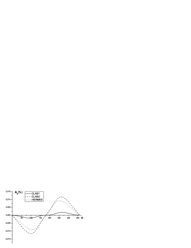
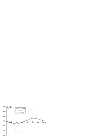
Figure 2: Dependence of the beam SSA (in per cent) on azimuth angle (in degrees) for three different experimental conditions (left panel): CLAS1 CLAS1 corresponds to $x=0.19,\ y=0.825,\ \rho=0.024,$ for CLAS2 CLAS2 $x=0.18,\ y=0.5,\ \rho=0.0185,$ and for HERMES HERMES $x=0.11,\ y=0.458,\ \rho=0.005.$ Curves for different values of $\rho$ on the right panel correspond to CLAS2 conditions CLAS2 .

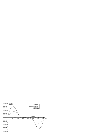
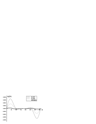
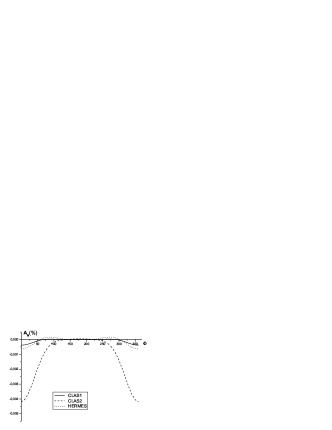
Figure 3: The target SSA as a function of azimuthal angle $\Phi$: For left panel, the polarization 4-vectors are defined by Eqs. (26) and the right panel corresponds to Eqs.(28).

III Target single–spin asymmetries

Let us now consider the target SSA in the process (1) caused by one–loop corrections to the unpolarized part of the leptonic tensor. In contrast with the beam single–spin correlation, where the effect is due to the real symmetrical part of the spin–dependent leptonic tensor, this time it is related with the imaginary antisymmetric part of the spin-independent leptonic tensor. In this case

$$A^{p}=\frac{\Re e[H^{S}_{\mu\nu}K^{(1)}_{\mu\nu}]}{B_{\mu\nu}H^{(un)}_{\mu\nu}}\ ,$$ (20)

where the effect is induced by the imaginary and antisymmetric part of the spin–independent tensor $K^{(1)}_{\mu\nu}$ that can be computed directly ($c.f.$ KMF ). Keeping only antisymmetric terms in $\mu\leftrightarrow\nu$, the result can be written as

$$K^{(1)}_{\mu\nu}=\frac{i\alpha}{4\pi}\Im m[(T_{12}-T_{21})(\tilde{k}_{1\mu}\tilde{k}_{2\nu}-\tilde{k}_{1\nu}\tilde{k}_{2\mu})]\ ,$$ (21)

where, neglecting terms proportional to $m^{2}$, we have

$$T_{12} = \frac{2}{st}\Big{[}\frac{\Delta^{2}}{s^{2}}c(u-s)G+\frac{\Delta^{2}}{t^{2}}(u\Delta^{2}-st)\widetilde{G}-2\Delta^{2}\big{(}\frac{u\Delta^{2}}{st}+\frac{2u-s+t}{a}L_{\Delta u}\big{)}+8u+3t-s+\frac{2us}{c}-$$ (22)

$$\frac{4(u^{2}-cs)(\Delta^{2}L_{\Delta u}-a)}{a^{2}}+\frac{\Delta^{2}(2c+t)(st-u\Delta^{2})L_{\Delta s}}{c^{2}t}-\frac{\Delta^{2}c(2u-s)L_{\Delta t}}{bs}\Big{]}\ ,$$

and $T_{21}$ is derived from $T_{12}$ by substitution $T_{21}=T_{12}(t\leftrightarrow s).$

After extracting absorptive parts from $L_{s}$ and $\widetilde{G}$ we obtain the following expression for antisymmetric imaginary part of the leptonic tensor (21):

$$K^{(1)}_{\mu\nu}=\frac{i\alpha}{2}(\tilde{k}_{1\mu}\tilde{k}_{2\nu}-\tilde{k}_{1\nu}\tilde{k}_{2\mu})T\ ,\ \ T=\frac{\Delta^{2}}{st}\Big{[}\frac{2st}{c^{2}}+4u\Big{(}\frac{1}{t}\ln\frac{u+t}{u}-\frac{1}{c}\Big{)}\Big{]}\ .$$ (23)

We note an overall factor of $\Delta^{2}$ from Eq.(23) that leads to additional suppression of target SSA in DVCS kinematics.

Contraction of the antisymmetric tensors in expression (20) for target SSA reads

$$H^{S}_{\mu\nu}K^{(1)}_{\mu\nu}=\alpha M(F_{1}+F_{2})TG_{s}\ ,$$ (24)

where the quantity $G_{s}$ depends on the target–proton polarization 4–vector $S$ and has the form

$$G_{s}=\Big{[}\Big{(}F_{1}+\frac{\Delta^{2}}{4M^{2}}F_{2}\Big{)}(k_{1}k_{2}\Delta S)+\frac{F_{2}}{2M^{2}}(p_{2}S)(k_{1}k_{2}\Delta p_{1})\Big{]}\ .$$ (25)

It follows from Eq. (25) that in general the one–loop correction to the leptonic tensor in radiative process (1) generates the target SSA due to all three possible orientations of the target polarization. Here we consider two possible conventions for defining directions of target polarization. First, one can consider the case when the longitudinal polarization (L) in laboratory system is along the electron beam direction of ${\bf k}_{1},$ transverse polarization (T) lies in the plane $({\bf k}_{1},{\bf k}_{2})$ and the normal (N) one is along the normal vector $({\bf k}_{1}\times{\bf k}_{2}).$ The corresponding polarization 4–vectors can be expressed via the 4–momenta Pol1

$$S^{L}_{1\mu}=\frac{2\tau k_{1\mu}-p_{1\mu}}{\sqrt{V\tau}}\ ,\ S^{N}_{1\mu}=-\frac{2(\mu k_{1}k_{2}p_{1})}{\sqrt{V^{3}xy\eta}}\ ,\ S^{T}_{1\mu}=\frac{k_{2\mu}-(1-y-2xy\tau)k_{1\mu}-xyp_{1\mu}}{\sqrt{Vxy\eta}}\ .$$ (26)

Then we have

$$G^{L}_{s1} = \frac{(k_{1}k_{2}\Delta p_{1})}{\sqrt{V\tau}}\Big{[}-F_{1}+\frac{F_{2}}{2}(\tilde{t}-xy)\Big{]}\ ,\ \ \tilde{t}=\frac{t}{V}\ ,$$ (27)

$$G^{T}_{s1} = \frac{(k_{1}k_{2}\Delta p_{1})}{\sqrt{Vxy\eta}}\Big{[}-xyF_{1}+\frac{F_{2}}{4\tau}\big{(}xy(1-y-2xy\tau)+\tilde{t}y(1+2x\tau)+\rho\big{)}\Big{]}\ ,$$

$$G^{N}_{s1} = -\frac{1}{4}\sqrt{\frac{V^{3}xy}{\eta}}\bigg{\{}\Big{(}F_{1}-\frac{\rho}{4\tau}F_{2}\Big{)}[xy(1-y)-\rho(1-xy)-(2-y)\tilde{t}]-\frac{4F_{2}(k_{1}k_{2}\Delta p_{1})^{2}}{V^{4}xy\tau}\bigg{\}}\ ,$$

with the same proton form factors $F_{1,2}$ as in Eqs.(5,6).

In another convention, one may choose directions to define the polarization 3–vector in the lab system. If the longitudinal direction is taken along ${\bf p}_{2},$ the transverse one in the plane $({\bf k}_{1},{\bf p}_{2})$ and the normal is along 3–vector ${\bf p}_{2}\times{\bf k}_{1},$ then the corresponding polarization 4–vector can be written as Pol2

$$S^{L}_{2\mu} = \frac{-2\tau\Delta_{\mu}-\rho p_{1\mu}}{\sqrt{V\tau\rho(4\tau+\rho)}}\ ,\ S^{N}_{2\mu}=-\frac{2(\mu p_{2}k_{1}p_{1})}{\sqrt{V^{3}\zeta}}\ ,\zeta=\rho(1-xy+\tilde{t})-\tau(xy-\tilde{t})^{2}\ ,$$ (28)

$$S^{T}_{2\mu} = \frac{\rho(4\tau+\rho)k_{1\mu}+(\rho-2\tau(\tilde{t}-xy)\Delta_{\mu}-\rho(2-xy+\tilde{t})p_{1\mu}}{\sqrt{V\zeta\rho(4\tau+\rho)}}\ .$$

In this case

$$G^{L}_{s2} = -\sqrt{\frac{\rho}{V\tau(4\tau+\rho)}}(k_{1}k_{2}\Delta p_{1})(F_{1}+F_{2})\ ,$$

$$G^{T}_{s2} = -\sqrt{\frac{\rho}{V\zeta(4\tau+\rho)}}(k_{1}k_{2}\Delta p_{1})(2-xy+\tilde{t})\Big{(}F_{1}-\frac{\rho}{4\tau}F_{2}\Big{)}\ ,$$ (29)

$$G^{N}_{2s} = \frac{1}{4}\sqrt{\frac{V^{3}}{\zeta}}\big{\{}\rho[\tilde{t}(1+xy)+xy(1-xy)]+y(\tilde{t}-xy)(\tilde{t}+x-xy)\Big{\}}\Big{(}F_{1}-\frac{\rho}{4\tau}F_{2}\Big{)}\ .$$

The target SSA in the BH process (1) is shown in Fig.3. Our calculations indicate that beam and target SSA generated by loop corrections to leptonic part of the interaction in the BH process are small and for the considered experimental conditions they do not exceed 0.1 per cent. The reason is that in addition to being multiplied by the fine structure constant $\alpha=\frac{1}{137}$, they contain additional suppression for the relevant values of kinematic invariants.

IV Summary

In conclusion, let us discuss the role of other radiative corrections in the BH process coming from real-photon radiation. In VCS experiments, the kinematic cuts are imposed in such a way that the phase space of the (undetected) additional photon is restricted to its relatively small values. In this case, the main contribution to the radiative correction comes from spin-independent soft photon emission that does not affect polarization observables, but does change unpolarized cross sections by as much as about 20 per cent (see, e.g., Mark for VCS case and Ref.Pol2 ; Afanasev:2001nn for elastic electron-proton scattering). Therefore in such a soft-photon-emission regime, the loop correction considered here is the only model-independent radiative correction to SSA.

Thus, we demonstrated that systematic corrections to beam and target SSA arising from the higher-order QED effects in the BH process are negligible compared to the relatively large (tens of per cent) experimentally observed asymmetries CLAS1 ; HERMES due to interference between the BH and VCS amplitudes in electroproduction of real photons. We confirm that the basic assumption of negligible SSA from the BH process alone holds to better than 0.1 per cent accuracy, thereby justifying present interpretation of SSA as arising mainly from the BH-VCS interference and VCS mechanisms.

References

• (1) Science Driving 12-GeV Upgrade of CEBAF, Jefferson Lab, Newport News, VA, February 2001, 294pp.
• (2) D. Műller et al., Fortshr. Phys. 42, 2 (1994); A.V. Radyushkin, Phys. Lett. B 385, 333 (1996); A.V. Radyushkin, Phys. Rev. D 56, 5524 (1997); X. Ji, Phys. Rev. Lett. 78, 610 (1997).
• (3) M. Diehl, Phys. Rept.  388, 41 (2003) [arXiv:hep-ph/0307382].
• (4) A. V. Belitsky and A. V. Radyushkin, arXiv:hep-ph/0504030.
• (5) H. Olsen and L. Maximon, Phys. Rev. 114, 887(1959).
• (6) W.R. Johnson, and J.D. Rozics, Phys. Rev. 128, 192 (1964); J.W. Motz, H. Olsen, and H.W. Koch, Rev. Mod. Phys. 36, 881 (1964); H. Kolbenstwedt, and H. Olsen, Nuovo Cim. 40, 13 (1964).
• (7) A.B. Arbuzov, E.A. Kuraev, N.P. Merenkov et al., Phys. Atom. Nucl., 59, 841 (1996).
• (8) M. Vanderhaegen et al., Phys. Rev. C 62, 025501 (2000).
• (9) E.A. Kuraev, N.P. Merenkov, V.S. Fadin, Sov. J. Nucl. Phys. 45, 1593 (1987).
• (10) S. Stepanyan [CLAS Collaboration], Phys. Rev. Lett.  87, 182002 (2001).
• (11) A. Airapetyan et al., Phys. Rev. Lett.  87, 182001 (2001).
• (12) E. S. Smith [CLAS Collaboration], AIP Conf. Proc.  698, 129 (2004) [arXiv:nucl-ex/0308032]; JLab Experiment E-01-113, Spokespersons: V. Burkert, L. Elouadrhiri, M. Garcon, and S. Stepanyan.
• (13) JLab Experiment E-00-110, Spokespersons: P. Bertin, C. Hyde-Wright, R. Ransome, and F. Sabatie.
• (14) N. d’Hose et al. Acta Phys. Polon. B 33, 3773 (2002).
• (15) A. V. Belitsky, D. Müller, A. Kirchner, Nucl. Phys. B 629, 323 (2002).
• (16) I. Akushevich, A. Arbuzov, and E. Kuraev, Phys. Lett. B 432 222, (1998).
• (17) A.V. Afanasev, I. Akushevich, N.P. Merenkov, J. Exp. Theor. Phys.  98, 403 (2004) [Zh. Eksp. Teor. Fiz.  98, 462 (2004)] [arXiv:hep-ph/0111331].
• (18) A.V. Afanasev, I. Akushevich, N.P. Merenkov, Phys. Rev. D, 65, 013006 (2002).
• (19) A. V. Afanasev, I. Akushevich, A. Ilyichev and N. P. Merenkov, Phys. Lett. B 514, 269 (2001).