Dalitz Plots and Hadron
Spectroscopy

Master Thesis

Faculty of Science, University of Bern

Author:

Adrian Wüthrich

May 2005

(July 2005: minor changes for publication on hep-ph)

Supervisor:

Prof. P. Minkowski

Institute for Theoretical Physics, University of Bern

CH-3012 Bern, Switzerland

Abstract

In this master thesis I discuss how the weak three-body decay $B^{+}\to\pi^{-}\pi^{+}K^{+}$ is related to the strong interactions between the final-state particles. Current issues in hadron spectroscopy define a region of interest in a Dalitz plot of this decay. This region is roughly characterized by energies from 0 to 1.6 GeV of the $\pi^{-}\pi^{+}$ and the $\pi^{-}K^{+}$ system, and energies from 3 to 5 GeV of the $\pi^{+}K^{+}$ system. Therefore I propose to use for the former two systems elastic unitarity (Watson’s theorem) as an approximate ansatz, and a non-vanishing forward-peaked amplitude for the latter system. I introduce most basic concepts in detail with the intention that this be of use to non-experts interested in this topic.

Chapter 1 Introduction

1.1 Dalitz plots and hadron spectroscopy

Dalitz plots are representations of a three-body decay,

$$X\to abc,$$ (1.1)

in a two-dimensional plot. The two axis of the plot are nowadays usually the invariant masses squared of two of the three possible particle pairs, i. e. for instance

$$\begin{split}s_{ab}&\equiv(p_{a}+p_{b})^{2},\\ s_{ac}&\equiv(p_{a}+p_{c})^{2}.\end{split}$$ (1.2)

One can also choose for the axis the invariant masses not squared or, as it was done mostly in the first Dalitz plots, the kinetic energies of two of the three decay products, for instance $T_{b}$ and $T_{c}$. These coordinates are equivalent in the sense that they are linearly related, e. g.

$$s_{ab}=m_{X}^{2}+m_{c}^{2}-2m_{X}(m_{c}+T_{c}).$$ (1.3)

Dalitz plots owe their name to Richard Dalitz who developed this representation technique in order to analyze the decay $K^{+}\to\pi^{+}\pi^{+}\pi^{-}$ [1, 2]. The basic idea is to assign each decay event its coordinates with respect to the two axis of the plot. One thus can obtain a “landscape” where the “mountains” correspond to a lot of events and the “valleys” to very few or no events.

1.1.1 “Old” and “new” Dalitz plots

Originally, the main application of Dalitz plots was to use it in order to determine spin and parity of the decaying particle. A prominent example is the decay

$$\omega^{0}\to\pi^{+}\pi^{0}\pi^{-},$$ (1.4)

see figure 1.1. Spin and parity of the decaying particle can be read off from characteristic patterns in the Dalitz plot as discussed prominently in ref. [4], see figure 1.2.

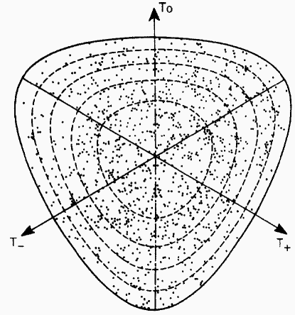
Figure 1.1: Dalitz plot for the decay $\omega^{0}\to\pi^{+}\pi^{0}\pi^{-}$, from [5] cited in [6, p. 320].

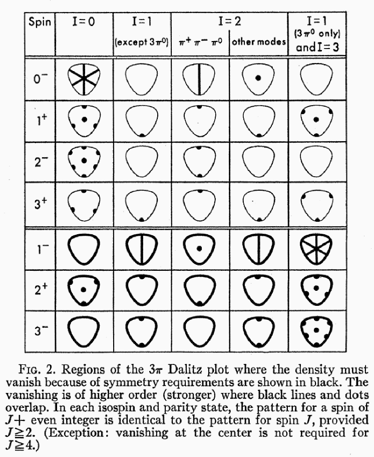
Figure 1.2: Characteristic patterns in a Dalitz plot from which spin and parity of the decaying particle can be determined; from [4].

In recent years Dalitz plots came to the fore again mainly in studies of $D$ and $B$ decays, see for instance [7] and [8]. These “new” Dalitz plots are distinguished from older Dalitz plots like the one in figure 2.1 by that they contain a number of events of 1000 to 2000, which reduces statistical fluctuations. Such modern Dalitz plots (figure 1.3) are therefore sensitive to the presence or absence of slight variations in the event distribution. Older Dalitz plots like the one in figure 2.1 could be used rather for “resonance hunting”. One searched for bands in the plot which can be associated to resonances.

Thanks to the sensitivity of the new Dalitz plots, they provide new input for problems in hadronic spectroscopy, see for instance [9] and [10].

Figure 1.3: A “modern” Dalitz plot of $B^{+}\to\pi^{-}\pi^{+}K^{+}$; from [8].

1.1.2 Issues in the spectroscopy of hadrons

Today’s controversial issues in hadron spectroscopy include the isoscalar scalars, more precisely the states with the quantum numbers of the vacuum,

$$J^{PC}=0^{++}.$$ (1.5)

One reason why these states are of particular interest is that two-pion exchange, which has $J^{PC}=0^{++}$, is the next-to-longest range contribution for the strong force [11, p. 1185]. The longest range contribution is the exchange of pions, the lightest hadrons. The isoscalar scalar sector is also relevant for glueballs. Various models (see references in [12]) predict the lightest glueball to have the quantum numbers of the vacuum.

To learn more about the scalars one investigates the component with total angular momentum $J=0$ (S wave) and isospin $I=0$ (iso-scalar) mainly of the $\pi\pi$ scattering amplitude, see figure 3.6, top panel. For the low energy region from zero to about 500 MeV there is Chiral Perturbation Theory that can state various results. However, the chiral expansion is hardly valid for energies up to about 1.6 GeV, which are to be taken into account in discussing the scalars.

The characteristic feature of $\pi\pi$ isoscalar S wave cross section, called red dragon by Minkowski and Ochs, can be explained by the negative interference of the $f_{0}(980)$ and the $f_{0}(1500)$ with the broad glueball with $J^{PC}=0^{++}$, [12]. Negative interference means that the rapid phase shift of $\pi$ does not start from zero as for a pure Breit-Wigner resonance but from a background phase of about already $\pi/2$ and then again from $3\pi/2$, see figure 3.7 on page 3.7. Alternative explanations postulate the $\sigma$ (also known as $f_{0}(600)$) and the $f_{0}(1370)$. The two alternatives yield at least to different scalar nonets as described in [9]:

• A scalar nonet with $f_{0}(980)$ and no lighter particles, including $a_{0}(980)$, $K_{0}^{*}(1430)$ and $f_{0}(1500)$, and

• a scalar nonet with $f_{0}(980)$ and no heavier particles, including $a_{0}(980)$, $\kappa(850)$ and $\sigma(600)$.

1.1.3 Weakly coupled decays and strong interactions

Remarkably enough, $\pi\pi$ scattering cannot be studied experimentally by scattering a pion beam off a pion target. This is impossible because of the short lifetime of about $10^{-8}$s for the charged pions and $10^{-16}$s for the neutral pion. A pion target would therefore have disappeared even before any scattering can happen. Chew and Low [13] proposed around 1960 a surrogate laboratory for unstable targets. Using basically the idea of Chew and Low a big part of the experimental input for $\pi\pi$ scattering comes from experiments such as $\pi p\to\pi\pi n$, see also section 5.2.3.

Another surrogate laboratory are three body decays. A prominent example is the decay $J/\psi\to\phi\pi\pi$. This is a process of the strong interaction but it is weakly coupled. More recently three-body decays by the weak interaction of $B$ and $D$ mesons have attracted attention. Dalitz plots from these decays that were produced in the first place for studies of CP violation serve with their high statistics as another source of a priori very precise experimental input. To use such Dalitz plots for the study of hadronic two-body scattering one has to relate the weak amplitude of the three-body decay to these hadronic amplitudes. To profit from the high statistics and to extract information not only from clearly visible peaks and dips it is important that the resulting ansatz for fitting the Dalitz plots is sensitive also to slight variations in the event distribution.

The ansatz that I will try to elaborate is guided by unitarity in two respects. For the amplitudes where we are interested in the energy region where at least approximately only the elastic channel is open, unitarity leads to a form of the decay amplitude that has the same phase as the strong interaction amplitude of the hadrons in the final state. This result is known as Watson’s theorem [15]. For the amplitude in higher energy regions inelastic channels have to be considered and the characteristic high energy behavior of the elastic amplitude may explain the main features. I will discuss whether for the high energy amplitude it is again unitarity that can be used to obtain via the optical theorem a rough idea of its behavior.

1.2 Outline

In chapter 2 I will introduce basic features of Dalitz plots. I will briefly discuss some points concerning background suppression. Then I will stress the possibility of interference between amplitudes and how in the presence of interference branching fractions are to be understood.

In chapter 3 the $S$ and $T$ matrix are defined. I discuss normalization and completeness of particle states, give formulations of unitarity conditions and derive the optical theorem. The detailed account of normalization allows me also to derive an equation defining the boundary of a Dalitz plot.

Chapter 4 deals with the kinematics of a three-body decay. There again one obtains equations for the boundary of a Dalitz plot. This time not through phase space considerations but through the definition of two-body subsystems in the three-body final state. These two-body subsystems are of interest because they can be related to the strong two-body scattering amplitudes in the final state and can be used to define alternative coordinate systems in a Dalitz plot appropriate for a partial-wave analysis.

In chapter 5 I will elaborate on the relation between the decay amplitude and the scattering amplitudes of the final state particles. For the scattering amplitudes I will first apply the constraints from unitarity (Watson’s theorem and the optical theorem). Then I try to see what consequences the known features of the (strong) two-body amplitudes have on an ansatz for the (weak) amplitude of the three-body decay.

Chapter 2 Background, resonances and interference

2.1 Background suppression

Consider as an example the study of the charmless $B^{+}\to K^{+}\pi^{+}\pi^{-}$ decay [16]. First, one has to detect the three particles with an appropriate detector. But not all $K$’s and $\pi$’s that are detected during the experiment may be produced in a charmless $B$ decay, and some particles may be misidentified as $K$’s and $\pi$’s.

The $K^{+}\pi^{+}\pi^{-}$ final states that come from other reactions than a $B$ decay can be vetoed by requiring that the total invariant mass of the three particles differ not much from the invariant mass of a $B^{+}$. By a similar criterion, then, one can further exclude the final states which are produced through a charmed (instead of charmless) $B$ decay (e. g. $B^{+}\to\bar{D}^{0}\pi^{+}$ followed by $\bar{D}^{0}\to K^{+}\pi^{-}$) [16, p. 7].

2.1.1 Sidebands

The final states where the invariant masses are in a certain neighborhood of the $B$ invariant mass belong to the signal region; other $K^{+}\pi^{+}\pi^{-}$ final states belong to the so-called sidebands. The events in the sidebands are background events. But not all events in the signal region are signal events, i. e. they do not all come from a charmless $B^{+}$ decay. In other words, not all background events are excluded by a sideband criterion. In particular, the background that comes from misidentification is still present. This sort of background is usually estimated by an extrapolation from the sidebands: When one has excluded all events from the sidebands region, the question remains which events in the signal region do still not come from a charmless $B^{+}\to K^{+}\pi^{+}\pi^{-}$ decay. To answer this question one may try the following procedure: Assume that the background that is not excluded by a restriction to the signal region comes only from misidentification. Try to estimate how much misidentified events there are in the sidebands. Assume that the same number of misidentified events is also present in the signal region. Subtract this number from the total events in the signal region and you will be left with events that indeed come from a charmless decay $B^{+}\to K^{+}\pi^{+}\pi^{-}$.

2.1.2 Background and correlations

A Dalitz plot analysis consists essentially in extracting information from deviations from homogeneous event distribution over the Dalitz plot. A band of higher than average density of events parallel to one of the axes, for instance, is the correlation between the four-momenta of two out of the three final state particles. The information one can extract under certain circumstances is that the two particles in question form a resonance. Another type of information extraction from correlations in this context is partial wave analysis.

In order to extract information from correlations one has to subtract the background in a way that does not give rise to correlations that are not due to the physics of the process. To avoid such spurious correlations one has to take care of two points in particular:

Partial wave decomposition of the background.

Also the background amplitudes should be decomposed into partial waves. This is often not done. As a positive example in this respect I can cite ref. [17], where the function that characterizes the acceptance of the detector is expanded in spherical harmonics.

Forming triplets of signal events.

A point in a Dalitz plot represents a triplet of signal pions and kaons that come from the same $B$. Assume that constraints like energy and momentum conservation or detection time do not determine which pions and kaons make up a Dalitz plot event. Assume as a simple example that there is a set of 8 $\pi^{-}$’s, a set of 7 $\pi^{+}$’s and a set of 9 $K^{+}$’s that are candidates for coming from the three-body decay of one of 5 $B^{+}$’s, see table 2.1. This means that the background estimation gives a ratio of signal to background of $5/8$, $5/7$ and $5/9$, respectively. Due to the possible quantum mechanical superposition of background and signal amplitudes it is impossible to say of an individual event whether it is a background or signal event and—if a signal event—from which of the 5 $B$’s it has come. But in order to avoid spurious correlations it is not sufficient just to fix the signal to background ratio of candidates for forming a Dalitz plot triplet. One must not form, for instance, pairs of pions for the $\pi^{-}\pi^{+}$ mass projection and $\pi^{-}K^{+}$ pairs for the $\pi^{-}K^{+}$ mass projection where the $K^{+}$ and the $\pi^{+}$ are not assigned to belong to the same Dalitz plot triplet. As an illustration see table 2.1.

$\pi^{-}$	$\pi^{+}$	$K^{+}$
		x
		x
		x
		x
		x
x	x	x
x	x	x
x		x
		x

$\pi^{-}$	$\pi^{+}$	$K^{+}$
x	x	x
x	x	x
x		x
x		x
x
x
x
x

$\pi^{-}$	$\pi^{+}$	$K^{+}$
x	x	x
x	x	x
x		x
		x

Table 2.1: An example of forming pairs for mass projections and Dalitz plot triplets that is consistent with a fixed signal to background ratio but can lead to spurious correlations.

2.1.3 Experimental difficulties

Particular experimental difficulties are encountered in obtaining a Dalitz plot in decays where one of the three decay products is a photon or where some decay products can further decay into photons, as in

$$J/\psi\to\gamma\pi\pi\qquad\text{and}\qquad B\to K\eta\pi.$$ (2.1)

The $J/\psi$ can also decay via a $\rho$ and a $\pi^{0}$ into a four-particle final state $\pi\pi\gamma\gamma$,

$$J/\psi\to\rho\pi^{0}\to(\pi\pi)(\gamma\gamma).$$ (2.2)

Photons escape quite easily any detection. If this happens the reaction $J/\psi\to\rho\pi^{0}\to(\pi\pi)(\gamma\gamma)$ is erroneously identified as a Dalitz plot event $J/\psi\to\gamma\pi\pi$; cf. [11, p. 1193], where these experimental difficulties are briefly recalled, and the work of the Mark III collaboration (e. g. ref. [18]), one of the most successful in overcoming these difficulties.

In the case of $B\to K\eta\pi$, on the other hand, the loss of a $\gamma$ may have as a consequence that a Dalitz plot event is not identified as such. This is because one way to detect the final state $\eta$ is via its subsequent decay into two photons.

2.2 Dalitz plots

2.2.1 Basic features

Dalitz plots have been introduced as a convenient method of analyzing reactions with three-body final-states in ref. [1], see also ref. [2]. Consider a three-particle final-state consisting of the three particles $abc$. Out of these three particles one has three possibilities to form a pair of two particles: $ab$, $ac$ and $bc$. For a Dalitz plot the invariant masses squared of two of the three pairs are represented as the two coordinate axes. Each of the three-body final-states produced in an experiment can be represented as a dot in the plane defined by these coordinate axes. Theoretically such dots are confined to a certain boundary depending on the kinematics of the reaction because outside this boundary the phase space volume is zero. For the interior of this boundary the phase space volume is constant, see section 3.3. Therefore, the density of the points inside the boundary is a constant multiple of the reaction matrix element squared. Thus, every structure in the density of the plots is due to dynamical characteristics of the reactions and not of kinematical origin.

If the reaction proceeds via an almost stable two-body intermediate state,

$$X\to(ab)c\to abc,$$ (2.3)

the three-body final states will be such that the distribution of the invariant mass of the pair $ab$ is centered around the invariant mass of the two-body intermediate state. This manifests itself in the Dalitz plot as a band of higher than average density of points, see figure 2.1.

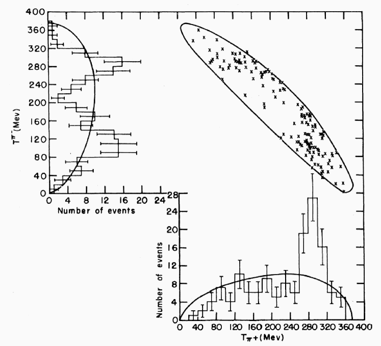
Figure 2.1: Bands in a Dalitz plot of $K^{-}p\to\pi^{\pm}\Lambda\pi^{\mp}$ due to the pion-lambda resonance $\Sigma^{\pm}(1385)$; from [19]. Also shown: Histograms of projections on the axis representing kinetic energies of two out of the three final-state particles.

A three-body decay $X\to abc$ has three two-body channels: $ab$, $ac$, and $bc$. If e. g. the pair $ab$ can form a quasi-stable state, a resonance, this appears in the Dalitz plot as a band along the region of the plot where the the two-particle invariant mass of the pair $ab$ is equal to the mass of the resonance. If e. g. the pair $ab$ may form a resonance, and one of the axes of the Dalitz plot is the invariant mass of the pair $ab$, then the band is perpendicular to this axis.

The same type of particle, say $ab$, may form more than one resonances. The various resonances then appear in the simplest case as parallel bands of a certain width in the Dalitz plot at respective positions given by the mass of the resonance. In general, interference effects can generate different structures.

2.2.2 Interference of a resonance with itself

Consider as an example of an interference effect a three-body decay where two of the three final-state particles are of the same type,

$$X\to abb.$$ (2.4)

Suppose further that a particle of type $a$ and a particle of type $b$ may form an almost stable intermediate state, a resonance $R^{*}$, say. Moreover, the channel via the resonance $R^{*}$ be the only process by which the particle of type $X$ decays into a particle of type $a$ and in two particles of type $b$. Then the decay amplitude is a superposition of two amplitudes: The intermediate state can be made up of the particle of type $a$ and one or the other particle of type $b$,

$$X\to\begin{array}[]{\{}{ccc}\}\rnode{A}{{\psframebox{a}}}&\rnode{B}{{\psframebox{b}}}&b{\psset{angleA=90.0}\ncbar{A}{B}}\\ \rnode{A}{{\psframebox{a}}}&b&\rnode{B}{{\psframebox{b}}}{\psset{angleA=-90.0}\ncbar{A}{B}}\end{array}\to abb.$$ (2.5)

In the Dalitz plot of such a three-body decay, with $m_{ab}$ of one combination $ab$ on one axis and $m_{ab}$ of the other combination on the other axis, there are two resonance bands perpendicular to one of the axes, respectively, at the position given by the mass of the resonance $R^{*}$. Depending on the kinematics of the process the two bands may or may not overlap. In case they do, there is constructive interference of the resonance amplitude in one of the two resonant two-body channels with the amplitude in the other. Thus in the region of the overlap the total intensity is not twice the intensity of an isolated band but four times because it is the amplitudes and not the intensities (i. e. the amplitudes squared) that are added. Two examples with even three overlapping bands are shown in figures 2.2 and 2.3. In figure 2.2 the bands are regions of higher than average density, i. e. peaks. In figure 2.3 the light blue bands due to the resonance $f_{0}(980)$ are regions with lower than average density, i. e. dips or valleys. Besides the overlap of bands this figure thus shows remarkably that resonances (here the $f_{0}(980)$) do not necessarily show up as peaks in a cross section.

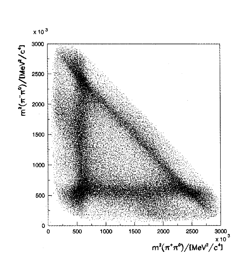
Figure 2.2: Overlapping bands showing the interference of the $\rho$ resonance with itself (different charge states) in $p\bar{p}\to\pi^{+}\pi^{-}\pi^{0}$; from [21] cited in [22, p. 36].

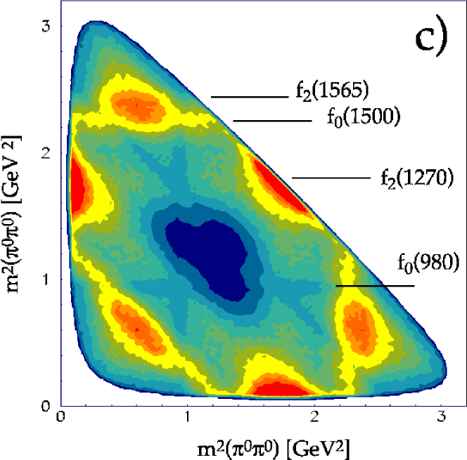
Figure 2.3: Overlapping of valleys due to the resonance $f_{0}(980)$ in $p\bar{p}\to 3\pi^{0}$; from [23]. Red and blue regions correspond respectively to high and low event densities.

2.3 Branching fractions

For a lot of unstable particles there is more than one possible decay product. A particle $X$ may e. g. decay in two particles $ab$, or $cd$, or in three particles $efg$. The probability for the particle $X$ to decay in one of the possible products is the respective branching fraction. The most likely decay could for example be $X\to ab$ with a probability of 80%. With 15% probability the particle $X$ may decay in the particle pair $cd$, and with 5% probability into $efg$. If there is only one possibility for the particle to decay, the branching fraction for this decay is 100% and for all other conceivable decays 0%—or one may prefer not to speak of branching fractions at all in such a case.

Dalitz plots can be used to determine branching fractions for three-body decays with almost stable two-body intermediate states. Consider as an example the following three-body decay that can proceed via three different resonances:

$$X\to\begin{array}[]{\{}{c}\}(ab)c\\ a(bc)\\ (ac)b\end{array}\to abc.$$ (2.6)

One may then ask what the respective probabilities are for these three possibilities. These probabilities are the (exclusive) branching fractions for the three processes respectively. The probability for the three-body decay $X\to abc$ to occur at all, i. e. via any intermediate state, is the inclusive branching fraction for the process $X\to abc$.

The task of determining branching fractions from a Dalitz plot may be seriously complicated by interference effects:

[…] we determine the exclusive branching fractions neglecting the effects of interference. The uncertainty due to possible interference between different intermediate states is included in the final result as a model-dependent error. […] We find that the model-dependent errors associated with the wide resonances introduce significant uncertainties into the branching fraction determination. [24]

2.3.1 Branching fractions, superposition and interference

The basic idea of branching fractions is to give a quantitative answer to the following type of questions. “If various processes are possible under given circumstances: How likely are the respective processes to occur?” Or: “If various processes could have occurred: How likely is it that one particular process has occurred?”

The quantum mechanical principle of superposition, however, implies that such types of questions do not always have an answer—except for the reply that the question is meaningless. This is for example the case in the notorious double slit experiment. If both slits are open as a matter of principle one cannot tell for a particular particle whether it has arrived at the screen via the upper or the lower slit. But still it seems that one can say something more about the intermediate state of a double slit experiment than just: “The particles arrived somehow at the screen.” In some sense the two possibilities (passing through the upper or lower slit) are on an equal footing. So one would like to say that it is equally probable that the particle has taken the upper slit or the lower slit, but at the same time, because the particle was in a state of superposition of the two possibilities, it has not taken one or the other route nor both. How can one solve the dilemma between superposition and the basic idea of a branching fraction? How can one define branching fractions in a sensible way even in the presence of superposition?

A possible solution is via an amplitude analysis. One can identify the intensity pattern as the square of a total amplitude which in turn decomposes into a sum of two amplitudes in the double slit case. One of these amplitudes represents the process via the upper slit the other amplitude represents the process via the lower slit. The respective squares of these two amplitudes are equal. It is in this sense that the two processes are on an equal footing. In this sense both processes (passing through the upper or lower slit) are equally probable although it is not the case that one or the other process has occurred but rather a superposition of both. Because the amplitudes of both processes contribute equally to the total amplitude the two processes should be assigned equal branching fractions, without interpreting this assignment as “in one half of a certain number of repetitions of the experiment the particle passes through the upper slit and in the other half of the repetitions through the lower slit”. Such an interpretation would be at odds with the superposition principle of (standard) quantum mechanics.

Let $\psi$ be the total amplitude of the process of a particle reaching the screen in the double slit setup, and $\psi_{1}$ and $\psi_{2}$ the amplitudes for passing through the upper or the lower slit, respectively,

$$\psi=\psi_{1}+\psi_{2}.$$ (2.7)

$|\psi|^{2}$ is the total intensity, which we set as unity of the branching fractions,

$$1=|\psi|^{2}=|\psi_{1}+\psi_{2}|^{2}=|\psi_{1}|^{2}+|\psi_{2}|^{2}+2\text{Re}(\psi_{1}\psi_{2}^{*}).$$ (2.8)

If as in the double slit experiment the two amplitudes interfere, we have $\text{Re}(\psi_{1}\psi_{2}^{*})\neq 0$, hence $|\psi_{1}|^{2}+|\psi_{2}|^{2}\neq 1$. This shows that when there is interference, branching fractions do in general not add up to unity.

The basic idea of branching fractions is to assign probabilities to various possibilities under given circumstances. Due to quantum mechanical superposition the totality of possibilities is not a complete set of alternatives in the sense of ordinary language, where exactly one of the alternatives is realized. If, moreover, the superposed amplitudes interfere the sum of all branching fractions is not one, which shows again, that it is not complete alternatives in the ordinary sense that branching fractions are assigned to.

2.3.2 Fit fractions in Dalitz plots

In Dalitz plots interference between resonant amplitudes show up as overlapping bands. As discussed in section 2.3.1, in the presence of interference the definition of a branching fraction is less obvious than it may seem at first sight. A very early determination of branching fractions from a Dalitz plot with two overlapping bands is ref. [25].

The method applied there is roughly the following. The mass projections of the Dalitz plot are fitted with a Breit-Wigner distribution without taking into consideration the events that fall in the overlap regions. The density of events in the resonance bands thus obtained is then extrapolated into the region of the overlap, assuming constant density of events in the resonance bands. The observed number of events in the overlap region is in good agreement with this extrapolation. This shows that the two overlapping resonances do not interfere. Therefore, the first fit can be corrected for the overlap regions assuming incoherent addition of the two amplitudes representing the overlapping bands.

But what about cases with interference? As mentioned at the beginning of section 2.3 the effect of interference on branching fractions is not always negligible. I cite again from ref. [24]:

We find that effects of interference between different two-body intermediate states can have significant influence on the observed two-particle mass spectra and a full amplitude analysis of the three-body $B$ meson decays is required for a more complete understanding. This will be possible with increased statistics.

It seems that recent experiments provide sufficient statistics to allow for such a full amplitude analysis [16, 26].

Chapter 3 Scattering amplitudes and particle states

3.1 $S$- and $T$-matrix

Let $|\alpha\rangle_{\text{in}}$ and $|\alpha\rangle_{\text{out}}$ be some appropriately defined states that are identical to the free-particle states $|\alpha\rangle$ (without subscript) in the respective limit $t\to-\infty$ $t\to+\infty$. The amplitude for the initial state $|\alpha\rangle_{\text{in}}$ to be found as the final state $|\alpha\rangle_{\text{out}}$ is given by the scalar products between these states. All possible scalar products can be collected in to rows and columns of a matrix, usually called $S$ (for scattering, I suppose).

$$S_{\alpha\beta}={{}_{\text{out}}\langle\alpha|\beta\rangle}_{\text{in}}.$$ (3.1)

We can define an operator $S$ such that sandwiched between free-particle states it yields the corresponding element of the $S$-matrix:

$$S_{\alpha\beta}=\langle\alpha|S|\beta\rangle.$$ (3.2)

The amplitude for the transition of state $|\beta\rangle$ to the state $|\alpha\rangle$ is the superposition of the amplitude $\langle\alpha|\beta\rangle$, which represents the quantum mechanical collapse of the state $|\beta\rangle$ in its component $|\alpha\rangle$, and an amplitude that represents a transition caused by some interaction. This latter amplitude is described in terms of the elements of the $T$-matrix

$$T_{\alpha\beta}=\langle\alpha|T|\beta\rangle,$$ (3.3)

such that

$$S_{\alpha\beta}=\langle\alpha|S|\beta\rangle=\langle\alpha|\beta\rangle+i\langle\alpha|T|\beta\rangle,$$ (3.4)

i. e. we define the $T$-matrix through the relation

$$S=\mathbbm{1}+iT.$$ (3.5)

3.2 Cross sections and decay rates

In this section I try to establish—in some detail but without going into the very foundations—the relation between the $T$ matrix elements and cross sections and decay rates. In particular I will focus on a decay of type $B^{+}\to abc$. The final result will be expressed in terms of matrix elements between state vectors characterized by their particle content and the four-momentum each particle has. Such states are improper vectors in an appropriately defined Hilbert space, and they owe their name to the fact that they lead in some context to undefined mathematical expressions. To avoid problems with improper vectors one can consider wave-packets instead of states with definite momentum. A slightly less expensive way is by normalizing the vectors with definite momentum with respect to a box of finite volume $V$; and by making explicit that the interaction that causes the decay is not present for an infinitely long time but only for a finite time $\tau$.

Both wave-packet and box approach have their respective advantages. In the box normalization the phase space factors are more clearly accounted for. To use the box normalization for the decay distribution of an instable particle faces, however, the inconsistency that the energy of the particle is assumed to be definite whereas a particle can only decay if it is not in an eigenstate of energy. In that respect it is more adequate to represent the initial state as a superposition of momentum eigenstates with nearly but not exactly the same eigenvalues, i. e. as a wave-packet.

3.2.1 Volume normalization

The state vectors $|B^{+},\vec{p}_{B}\rangle$ are considered as plane wave functions

$$\Psi(t,\vec{x})=\mathcal{N}e^{iEt}e^{-i\vec{p}\vec{x}}.$$ (3.6)

The absolute squares of these wave functions represent a probability density and have therefore to be normalized to unity. I will do this with respect to a volume $V=L^{3}$. Therefore the method shown here is also known as box normalization. Choosing the volume to be a box makes the calculations easier. The idea of normalizing states to a finite volume, however, does not only apply to this special choice of volume. The normalization constant $\mathcal{N}$ is determined by

$$1=\int_{V}d^{3}x\,|\Psi(t,\vec{x})|^{2}=\mathcal{N}^{2}\int_{V}d^{3}x=V$$ (3.7)

to be

$$\mathcal{N}=\frac{1}{\sqrt{V}}.$$ (3.8)

In a box of finite volume $V$ the three-momenta are discrete if one imposes periodic boundary conditions

$$\Psi_{p}(t;(0,x_{2},x_{3})) =\Psi_{p}(t;(L,x_{2},x_{3})),$$ (3.9)

$$\Psi_{p}(t;(x_{1},0,x_{2})) =\Psi_{p}(t;(x_{1},L,x_{3})),$$ (3.10)

$$\Psi_{p}(t;(x_{1},x_{2},0)) =\Psi_{p}(t;(x_{1},x_{2},L)).$$ (3.11)

Then one has, for instance,

$$\Psi_{p}(t;(0,x_{2},x_{3}))=\frac{1}{\sqrt{V}}e^{iEt}e^{-i(p_{2}x_{2}+p_{3}x_{3})}=\frac{1}{\sqrt{V}}e^{iEt}e^{-i(p_{1}L+p_{2}x_{2}+p_{3}x_{3})}\\ =e^{-ip_{1}L}\Psi_{p}(t;(0,x_{2},x_{3})),$$ (3.12)

which requires the eigenvalues for $\vec{p}$ to be quantized, i. e. labeled by a triplet of integers $\vec{n}\in\mathbb{Z}^{3}$,

$$\vec{p}=\frac{2\pi}{L}\vec{n}.$$ (3.13)

Because the plane wave functions are normalized to unity, the scalar product between the momentum states in the box is a Kronecker delta,

$$\langle\vec{p}(\vec{n}^{\prime})|\vec{p}(\vec{n})\rangle=\int_{V}d^{3}x\,\Psi_{\vec{n}^{\prime}}(t,\vec{x})\Psi_{\vec{n}}^{*}(t,\vec{x})\\ =\frac{1}{V}\int_{V}d^{3}x\,\exp(-i(\vec{p}(\vec{n}^{\prime})-\vec{p}(\vec{n}))\vec{x})=\delta^{3}_{\vec{n}^{\prime}\vec{n}}.$$ (3.14)

Be $|f\rangle_{\text{box}}$ and $|i\rangle_{\text{box}}$ a state of $m_{f}$ ($m_{i}$) particles each with three-momenta $\vec{p}_{m_{f}}$ ($\vec{p}_{m_{i}}$), normalized to the box of volume $V$. (Multi-particle states are direct products of one-particle states.) The transition probability from $|i\rangle_{\text{box}}$ to $|f\rangle_{\text{box}}$ is given by

$$\Delta w(f,i)=|_{\text{box}}\langle f|S|i\rangle_{\text{box}}|^{2}=|_{\text{box}}\langle f|i\rangle_{\text{box}}+i_{\text{box}}\langle f|T|i\rangle_{\text{box}}|^{2}=|_{\text{box}}\langle f|T|i\rangle_{\text{box}}|^{2}.$$ (3.15)

The probability for a transition of $|i\rangle_{\text{box}}$ into any momentum configuration is

$$w(f,i)=\prod_{m_{f}}\sum_{\vec{n}_{m_{f}}}|_{\text{box}}\langle f|T|i\rangle_{\text{box}}|^{2}\\ =\prod_{m_{f}}\frac{V}{(2\pi)^{3}}\sum_{\vec{n}_{m_{f}}}\frac{(2\pi)^{3}}{V}|_{\text{box}}\langle f|T|i\rangle_{\text{box}}|^{2}\\ =\left(\frac{V}{(2\pi)^{3}}\right)^{m_{f}}\left(\prod_{m_{f}}\int d^{3}p_{m_{f}}\,\right)|_{\text{box}}\langle f|T|i\rangle_{\text{box}}|^{2},$$ (3.16)

where in the last step I performed the limit $L\to\infty$, using Riemann’s definition of the integral and equation (3.13). What is the appropriate expression for ${}_{\text{box}}\langle f|T|i\rangle_{\text{box}}$ in the limit of large volume (i. e. $L\to\infty$)? We want the continuous momentum eigenstates to be normalized as

$$\begin{split}\langle f^{\prime}|f\rangle&=\prod_{m_{f}}(2\pi)^{3}2E_{m_{f}}\delta^{3}(\vec{p}^{\prime}_{m_{f}}-\vec{p}_{m_{f}})\\ &=\prod_{m_{f}}2E_{m_{f}}\int d^{3}x\,\exp(-i(\vec{p}^{\prime}_{m_{f}}-\vec{p}_{m_{f}})\vec{x}),\end{split}$$ (3.17)

and similarly for $\langle i^{\prime}|i\rangle$. In the limit of large volume the right-hand side of equation (3.17) is

$$\prod_{m_{f}}2E_{m_{f}}\int d^{3}x\,\exp(-i(\vec{p}^{\prime}_{m_{f}}-\vec{p}_{m_{f}})\vec{x})\\ =\prod_{m_{f}}2E_{m_{f}}\int_{V}d^{3}x\,\exp(-i(\vec{p}(\vec{n}^{\prime}_{m_{f}})-\vec{p}(\vec{n}_{m_{f}}))\vec{x})\\ =\prod_{m_{f}}2E_{m_{f}}V\delta^{3}_{\vec{n}^{\prime}\vec{n}}=\prod_{m_{f}}2E_{m_{f}}V\langle\vec{p}_{m_{f}}(\vec{n}^{\prime}_{m_{f}})|\vec{p}_{m_{f}}(\vec{n}_{m_{f}})\rangle\\ =V^{m}\left(\prod_{m_{f}}2E_{m_{f}}\right){{}_{\text{box}}}\langle f^{\prime}|f\rangle_{\text{box}}.$$ (3.18)

It follows that

$$|f\rangle_{\text{box}}=\left(\prod_{m_{f}}\sqrt{\frac{(2\pi)^{3}}{2E_{m_{f}}V}}\right)|f\rangle,$$ (3.19)

and similarly for $|i\rangle$ such that

$${}_{\text{box}}\langle f|T|i\rangle_{\text{box}}=\left(\prod_{m_{f}}\sqrt{\frac{(2\pi)^{3}}{2E_{m_{f}}V}}\right)\left(\prod_{m_{i}}\sqrt{\frac{(2\pi)^{3}}{2E_{m_{i}}V}}\right)\langle f|T|i\rangle,$$ (3.20)

and therefore from equation (3.16)

$$w(f,i)=\left(\prod_{m_{i}}\frac{(2\pi)^{3}}{2E_{m_{i}}V}\right)\left(\prod_{m_{f}}\int\frac{d^{3}p_{m_{f}}}{2E_{m_{f}}}\right)|\langle f|T|i\rangle|^{2}.$$ (3.21)

$T$ conserves energy and momentum. $T$ is zero whenever the energy and momentum of the final and initial state are different. It is therefore suitable to consider the multi-particle states $|i\rangle$ (and $|f\rangle$) as direct products of eigenstates of the total four-momentum and a vector $|\psi\rangle$ which contains all the remaining characteristics of the multi-particle state, such as the masses, three-momenta and quantum numbers of each particle in the state,

$$|i\rangle=|p_{\text{tot}}^{(i)}\rangle\otimes|\psi_{i}\rangle.$$ (3.22)

Since $T$ conserves the total four-momentum it acts as the unit operator in the space of eigenstates of total four-momentum and thus takes the following form as a direct product,

$$T=\mathbbm{1}\otimes\mathcal{M}.$$ (3.23)

The $T$ elements between final and initial states then look like

$$\langle f|T|i\rangle=\langle p_{\text{tot}}^{(f)}|\mathbbm{1}|p_{\text{tot}}^{(i)}\rangle\langle\psi_{f}|\mathcal{M}|\psi_{i}\rangle=\delta^{4}(p_{i}-p_{f})\langle\psi_{f}|\mathcal{M}|\psi_{i}\rangle\equiv\delta^{4}(p_{i}-p_{f})\mathcal{M}_{fi}.$$ (3.24)

In terms of $\mathcal{M}$ we have

$$w(f,i)=\left(\prod_{m_{i}}\frac{(2\pi)^{3}}{2E_{m_{i}}V}\right)\left(\prod_{m_{f}}\int\frac{d^{3}p_{m_{f}}}{2E_{m_{f}}}\right)[\delta^{4}(p_{B}-p_{\text{tot}})]^{2}|\mathcal{M}_{fi}|^{2}.$$ (3.25)

To make sense of the two delta-functions we write for one of it its integral representation in the volume and time interval that is large but explicitly accounted for. To be explicit in this subtle point I consider the delta-functions explicitly as distributions in a space of test-functions $f(p_{f})$.

$$\int d^{4}p_{f}\,[\delta^{4}(p_{i}-p_{f})]^{2}f(p_{f})\\ =\int d^{4}p_{f}\,\delta^{4}(p_{i}-p_{f})\frac{1}{(2\pi)^{4}}\int_{V\tau}d^{4}x\,\exp(-i(p_{i}-p_{f})x)f(p_{f})\\ =\frac{1}{(2\pi)^{4}}\int_{V\tau}d^{4}x\,f(p_{i})=\frac{V\tau}{(2\pi)^{4}}f(p_{i})\\ =\int d^{4}p_{f}\,\frac{V\tau}{(2\pi)^{4}}\delta^{4}(p_{i}-p_{f})f(p_{f}).$$ (3.26)

In the usual short-hand notation this reads

$$[\delta^{4}(p_{i}-p_{f})]^{2}=\frac{V\tau}{(2\pi)^{4}}\delta^{4}(p_{i}-p_{f}).$$ (3.27)

Equation (3.25) then yields

$$w(f,i)=\left(\prod_{m_{i}}\frac{1}{2E_{m_{i}}}\right)\frac{V^{1-m_{i}}}{(2\pi)^{3m_{i}-4}}\,\tau\int dQ\,|\mathcal{M}_{fi}|^{2},$$ (3.28)

with

$$dQ\equiv\delta^{4}(p_{i}-p_{f})\prod_{m_{f}}\frac{d^{3}p_{m_{f}}}{2E_{m_{f}}}$$ (3.29)

the phase space volume for a final state containing $m_{f}$ particles. Usually the quantity of interest is the rate, i. e. the transition probability per interaction time $\tau$

$$\Gamma(f,i)=\frac{w(f,i)}{\tau}=\left(\prod_{m_{i}}\frac{1}{2E_{m_{i}}}\right)\frac{V^{1-m_{i}}}{(2\pi)^{3m_{i}-4}}\,\int dQ\,|\mathcal{M}_{fi}|^{2}.$$ (3.30)

$\boldsymbol{m_{i}=1}$ (decay)

In the case of $m_{i}=1$ equation (3.28) reads

$$w(f,i)=\frac{1}{2E}2\pi\tau\int dQ\,|\mathcal{M}_{fi}|^{2}.$$ (3.31)

According to this equation the transition probability for decay should increase proportional to the interaction time $\tau$. However, when the particle has decayed the probability of decay should be zero. So equation (3.31) is only valid for $\tau$ much less than the mean lifetime of the decaying particle. This conflicts with the assumption of very large $\tau$ when representing the $\delta^{4}$ functions as an integral over space-time. Also formula (3.31) contains a factor $2E$, where $E$ is the energy of the decaying particle. However, as mentioned at the beginning of this section, a particle only decays if it has no sharp energy value. These problems can be avoided when the initial particle is represented by a wave packet, see section 3.2.2.

$\boldsymbol{m_{i}=2}$ (two-body scattering)

With $m_{i}=2$ equation (3.30) is

$$\Gamma(f,i)=\frac{w(f,i)}{\tau}=\frac{1}{2E_{1}2E_{2}}\frac{1}{V(2\pi)^{2}}\,\int dQ\,|\mathcal{M}_{fi}|^{2}.$$ (3.32)

The cross section is defined as rate per flux. In the cms ($\vec{p}_{1}=-\vec{p}_{2}\equiv p\vec{p}_{1}/|\vec{p}_{1}|$) the flux is given by ($\rho$: particle density, $v$: relative velocity between beam and target particle)

$$\Phi=\rho v=\frac{v}{V}=\frac{|\vec{v}_{1}-\vec{v}_{2}|}{V}=\frac{|\vec{p}_{1}/E_{1}-\vec{p}_{2}/E_{2}|}{V}=\frac{p(E_{1}+E_{2})}{E_{1}E_{2}V},$$ (3.33)

and

$$s\equiv(p_{1}+p_{2})^{2}=(E_{1}+E_{2})^{2}-(\vec{p_{1}}+\vec{p_{2}})^{2}=(E_{1}+E_{2})^{2},$$ (3.34)

such that the cross section for scattering of two spinless particles into a final state containing $m_{f}$ particles characterized by a set of quantum numbers $\Lambda$ reads

$$\sigma_{\Lambda}(2\to m_{f})=\frac{\Gamma(f,i)}{\Phi}=\frac{1}{16\pi^{2}p\sqrt{s}}\int dQ_{m_{f}}\,|\mathcal{M}_{(f_{\Lambda})i}|^{2}.$$ (3.35)

The total cross section is the sum over

• all numbers of particles $M(\sqrt{s})$ that can be produced at a given cms energy $\sqrt{s}$, and

• for each number of particles all (accessible) set of quantum numbers $\Lambda$,

$$\sigma_{\text{tot}}=\sigma(2\to\text{anything})=\sum_{m_{f}=2}^{M}\sum_{\Lambda}\sigma_{\Lambda}(2\to m_{f}),$$ (3.36)

where $M(s)$ is maximal number of particles that can be produced at a given center of mass energy $\sqrt{s}$. Using “anything” in this sense, I adopted the following normalization and completeness relation (cf. eq. (3.17)),

$$\langle p_{1},\ldots,p_{m_{f}};\Lambda_{m_{f}}|p_{1}^{\prime},\ldots,p_{m_{f}}^{\prime};\Lambda_{m_{f}}^{\prime}\rangle=\delta_{{m_{f}}{m_{f}^{\prime}}}\prod_{m_{f}}(2\pi)^{3}2E_{m_{f}}\delta^{3}(\vec{p}^{\prime}_{m_{f}}-\vec{p}_{m_{f}})\delta_{\Lambda_{m_{f}},\Lambda_{m_{f}}^{\prime}},$$ (3.37)

$$\begin{split}\mathbbm{1}&=\sum_{m_{f}}\prod_{m_{f}}\int\frac{d^{3}p_{m_{f}}}{2E_{m_{f}}}\sum_{\Lambda_{m_{f}}}|p_{1},\ldots,p_{m_{f}};\Lambda_{m_{f}}\rangle\langle p_{1},\ldots,p_{m_{f}};\Lambda_{m_{f}}|\\ &=\sum_{m_{f}}\int d^{4}p_{\text{tot},m_{f}}\int dQ_{m_{f}}\,\sum_{\Lambda_{m_{f}}}|p_{\text{tot}}\rangle|\psi\rangle\langle p_{\text{tot}}|\langle\psi|\\ &\equiv\sum_{m_{f}}\left[\int d^{4}p_{\text{tot},m_{f}}|p_{\text{tot}}\rangle\langle p_{\text{tot}}|\otimes\int d\psi\,|\psi\rangle\langle\psi|\right]\\ &\equiv\int d\beta\,|\beta\rangle\langle\beta|.\end{split}$$ (3.38)

The total cross section then can be written as

$$\sigma_{\text{tot}}=\frac{1}{16\pi^{2}p\sqrt{s}}\sum_{m_{f}=2}^{M}\sum_{\Lambda}\int dQ_{m_{f}}\,|\mathcal{M}_{(f_{\Lambda})i}|^{2}.$$ (3.39)

We further have with $p_{f}$ and $p_{i}$ the total four-momentum of the final and initial state respectively (cf. equation (3.52) and following)

$$\sum_{m_{f}=2}^{M}\sum_{\Lambda}\int dQ_{m_{f}}\,=\int d^{4}p_{f}\,\delta^{4}(p_{i}-p_{f})\sum_{m_{f}=2}^{M}\sum_{\Lambda}\int dQ_{m_{f}}.$$ (3.40)

Therefore,

$$\sigma_{\text{tot}}=\frac{1}{16\pi^{2}p\sqrt{s}}\int d\beta\,|\langle\beta|T|i\rangle|^{2}.$$ (3.41)

3.2.2 Wave packets

To obtain the relation between the respective $T$-matrix elements and the decay distribution of $B^{+}\to\pi^{-}\pi^{+}K^{+}$ I follow the lines of [27, p. 140ff.], which they use to define the scattering cross section of two particles.

Let $|\alpha\rangle$ be the state vector that represents a collection of $B^{+}$’s with a four-momentum distribution $\phi(p_{B})$.

$$|\alpha\rangle=\int d^{4}p_{B}\delta(p_{B}^{2}-m_{B}^{2})\theta(p_{B}^{0})\phi(p_{B})|B^{+},p_{B}\rangle.$$ (3.42)

If we consider a collection of $B^{+}$’s at rest, $\phi(p_{B})$ will be narrowly centered around $p_{B}=(m_{B},0,0,0)$, where $m_{B}$ is the $B$ mass of around 5.279 GeV. The four-momentum eigenvectors $|B^{+},p_{B}\rangle$ are normalized as

$$\langle B^{+},p^{\prime}|B^{+},p\rangle=2p_{B}^{0}\delta^{3}(\vec{p}-\vec{p}^{\prime}),$$ (3.43)

and the norm of the state $|\alpha\rangle$ is the time derivative of the particle number density

$$N_{B}=\int dt\langle\alpha|\alpha\rangle,$$ (3.44)

where $N_{B}$ is the number of $B^{+}$’s produced in the experiment.

$S$-, $T$- and $\mathcal{M}$-matrices are defined by

$$S=\mathbbm{1}+iT=\mathbbm{1}+i\delta^{4}(p_{B}-p_{\text{tot}})\mathcal{M},$$ (3.45)

where $p_{\text{tot}}=\sum_{i}p_{i}$.

The transition amplitude for the $B$ to decay in a three-body state $|\beta\rangle=|\pi^{-},p_{1};\pi^{+},p_{2};K^{+},p_{3}\rangle$ of definite momenta of the three decay products is given by

$$\langle\beta|S|\alpha\rangle=i\langle\beta|T|\alpha\rangle.$$ (3.46)

The probability for a decay into a volume of momentum space is the square of this amplitude integrated with the appropriate measure (see [27, p. 141])

$$\begin{split}P(B;p_{1},p_{2},p_{3})&=\int_{\vec{p}_{1}}^{\vec{p}_{1}+\vec{k}_{1}}\frac{d^{3}p_{1}}{2p_{1}^{0}}\int_{\vec{p}_{2}}^{\vec{p}_{2}+\vec{k}_{2}}\frac{d^{3}p_{2}}{2p_{2}^{0}}\int_{\vec{p}_{3}}^{\vec{p}_{3}+\vec{k}_{3}}\frac{d^{3}p_{3}}{2p_{3}^{0}}\\ &\quad\times\int d^{4}p_{B}\,d^{4}p_{B}^{\prime}\delta(p_{B}^{2}-m_{B}^{2})\theta(p_{B}^{0})\phi(p_{B})\\ &\quad\times\delta({p_{B}^{\prime}}^{2}-m_{B}^{2})\theta({p_{B}^{0}}^{\prime})\phi^{*}(p^{\prime}_{B})\\ &\quad\times\langle B^{+},p^{\prime}_{B}|T^{\dagger}|\alpha\rangle\langle\alpha|T|B^{+},p_{B}\rangle.\end{split}$$ (3.47)

The measure has to do with the normalization of equation (3.43). To simplify this expression by an approximation it is useful to express it in term of elements of $\mathcal{M}$. We have

$$\langle\beta|T|\alpha\rangle=\int d^{4}p_{B}\delta(p_{B}^{2}-m_{B}^{2})\theta(p_{B}^{0})\phi(p_{B})\delta^{4}(p_{B}-p_{\text{tot}})\langle\beta|\mathcal{M}|B^{+},p_{B}\rangle.$$ (3.48)

If the momentum distribution $\phi(p_{B})$ is sufficiently narrow, we can approximate the above expression by assuming that the $\mathcal{M}$ element is independent of $p_{B}$ and that it can therefore be pulled outside the integral. For the decay probability we then obtain

$$\begin{split}P(B;p_{1},p_{2},p_{3})&=\int_{\vec{p}_{1}}^{\vec{p}_{1}+\vec{k}_{1}}\frac{d^{3}p_{1}}{2p_{1}^{0}}\int_{\vec{p}_{2}}^{\vec{p}_{2}+\vec{k}_{2}}\frac{d^{3}p_{2}}{2p_{2}^{0}}\int_{\vec{p}_{3}}^{\vec{p}_{3}+\vec{k}_{3}}\frac{d^{3}p_{3}}{2p_{3}^{0}}\\ &\quad\times|\langle\beta|\mathcal{M}|B^{+},p_{B}\rangle|^{2}\int d^{4}p_{B}\,d^{4}p_{B}^{\prime}\delta(p_{B}^{2}-m_{B}^{2})\theta(p_{B}^{0})\phi(p_{B})\\ &\quad\times\delta({p_{B}^{\prime}}^{2}-m_{B}^{2})\theta({p_{B}^{0}}^{\prime})\phi^{*}(p^{\prime}_{B})\delta^{4}(p_{B}-p_{\text{tot}})\delta^{4}(p^{\prime}_{B}-p_{\text{tot}}).\end{split}$$ (3.49)

For further simplification I introduce the Fourier-transforms of the momentum distributions,

$$\Phi(x)=\int d^{4}p_{B}\delta(p_{B}^{2}-m_{B}^{2})\theta(p_{B}^{0})\phi(p_{B})e^{ip_{B}x}.$$ (3.50)

After some algebra one arrives then at

$$\begin{split}P(B;p_{1},p_{2},p_{3})&=\int_{\vec{p}_{1}}^{\vec{p}_{1}+\vec{k}_{1}}\frac{d^{3}p_{1}}{2p_{1}^{0}}\int_{\vec{p}_{2}}^{\vec{p}_{2}+\vec{k}_{2}}\frac{d^{3}p_{2}}{2p_{2}^{0}}\int_{\vec{p}_{3}}^{\vec{p}_{3}+\vec{k}_{3}}\frac{d^{3}p_{3}}{2p_{3}^{0}}\\ &\quad\times|\langle\beta|\mathcal{M}|B^{+},p_{B}\rangle|^{2}(2\pi)^{-8}\int d^{4}x\int d^{4}y\Phi(x)\Phi^{*}(y)e^{-ip_{\text{tot}}(x-y)}.\end{split}$$ (3.51)

The integrations in the space of final state momenta can be written as

$$\prod_{i=1}^{3}\int_{\vec{p}_{i}}^{\vec{p}_{i}+\vec{k}_{i}}\frac{d^{3}p_{i}}{2E_{i}}=\int d^{4}p_{\text{tot}}\,dQ_{3}$$ (3.52)

with

$$dQ_{3}=\prod_{i=1}^{3}\int_{\vec{p}_{i}}^{\vec{p}_{i}+\vec{k}_{i}}\frac{d^{3}p_{i}}{2E_{i}}\delta^{4}(p_{1}+p_{2}+p_{3}-p_{\text{tot}}).$$ (3.53)

This can be checked using a test functions

$$f(\sum_{i}E_{i},\sum_{i}\vec{p}_{i},\vec{p}_{1},\vec{p}_{2},\vec{p}_{3}))\equiv\tilde{f}(\vec{p}_{1},\vec{p}_{2},\vec{p}_{3})$$ (3.54)

as follows ($p_{\text{tot}}=\sum_{i=1}^{3}p_{i}$, $E_{i}=\sqrt{m_{i}^{2}+\vec{p}_{i}^{2}}$):

$$\int d^{4}p_{\text{tot}}\,dQ_{3}f(p^{0}_{\text{tot}},\vec{p_{\text{tot}}},\vec{p}_{1},\vec{p}_{2},\vec{p}_{3})=\\ \prod_{i=1}^{3}\int_{\vec{p}_{i}}^{\vec{p}_{i}+\vec{k}_{i}}\frac{d^{3}p_{i}}{2E_{i}}f(\sum_{i}E_{i},\sum_{i}\vec{p}_{i},\vec{p}_{2},\vec{p}_{3})=\\ \prod_{i=1}^{3}\int_{\vec{p}_{i}}^{\vec{p}_{i}+\vec{k}_{i}}\frac{d^{3}p_{i}}{2E_{i}}\tilde{f}(\vec{p}_{1},\vec{p}_{2},\vec{p}_{3}).$$ (3.55)

If we integrate over all values of $p_{\text{tot}}$ the above equality is not exact. However, we will use this equality to evaluate expressions such as that in equation (3.49). There we assume the momentum distribution function $\phi(p_{B})$ to be narrowly centered around a certain value ($(m_{B},0,0,0)$ in the $B$ rest system). Because of the factors $\delta^{4}(p_{B}-p_{\text{tot}})\delta^{4}(p^{\prime}_{B}-p_{\text{tot}})$ the integrand in equation (3.49) vanishes unless $p_{\text{tot}}=p_{1}+p_{2}+p_{3}$ takes on values near the central value of $p_{B}$. So the mistake we make by integrating over all values of $p_{\text{tot}}$ can be made arbitrarily small by making the momentum distributions arbitrarily narrow.

We can now make the substitution of equation (3.55) in equation (3.51) and perform the integration over $p_{\text{tot}}$. This gives

$$P(B;p_{1},p_{2},p_{3})=\int dQ_{3}|\langle\beta|\mathcal{M}|B^{+},p_{B}\rangle|^{2}(2\pi)^{-4}\int d^{4}x|\Phi(x)|^{2}.$$ (3.56)

By Fourier-transforming back $\Phi(x)$, using

$$\begin{split}d^{4}p\delta(p^{2}-m^{2})\theta(p^{0})&=d^{3}pdp^{0}\delta({p^{0}}^{2}-(\vec{p}^{2}+m^{2}))\\ &=d^{3}pdp^{0}\frac{1}{2\sqrt{\vec{p}^{2}+m^{2}}}\theta(p^{0})\\ &\quad\times\left[\delta\left(p^{0}+\sqrt{\vec{p}^{2}+m^{2}}\right)+\delta\left(p^{0}-\sqrt{\vec{p}^{2}+m^{2}}\right)\right]\theta(p^{0})\\ &=\frac{d^{3}p}{2p^{0}}\end{split}$$ (3.57)

and assuming once more that the momentum distributions are narrow one can show that

$$\int d^{3}x\,|\Phi(x)|^{2}=\frac{(2\pi)^{3}}{p^{0}_{B}}\langle\alpha|\alpha\rangle=\frac{(2\pi)^{3}}{p^{0}_{B}}\frac{dN_{B}}{dt},$$ (3.58)

where the last equality is equivalent to equation (3.44). The particle density $\rho(x)$ is then

$$\rho(x)=\frac{p^{0}_{B}}{(2\pi)^{3}}|\Phi(x)|^{2},$$ (3.59)

such that

$$N_{B}=\int d^{4}x\,\rho(x)$$ (3.60)

is the total number of $B$’s produced in the experiment.

Thus equation (3.56) reads

$$P(B;p_{1},p_{2},p_{3})=\frac{N_{B}}{2\pi p^{0}_{B}}\int dQ_{3}|\langle\beta|\mathcal{M}|B^{+},p_{B}\rangle|^{2}.$$ (3.61)

The differential number of decay events that yield decay products in the momentum volume $dQ_{3}$ can be read off to be

$$\frac{dP(B;p_{1},p_{2},p_{3})}{dQ_{3}}=\frac{N_{B}}{2\pi p^{0}_{B}}|\langle\beta|\mathcal{M}|B^{+},p_{B}\rangle|^{2}.$$ (3.62)

In this way the $\mathcal{M}$-elements between momentum eigenstates determine the decay distribution of the $B$ meson that is characterized by $\phi(p_{B})$ as a wave packet.

3.3 Three-body phase space in a Dalitz plot

In this section I try to show, that the phase space volume $\int dQ_{3}$ is constant over the Dalitz plot. There are alternative proofs in the literature, e. g. [3, p. 140f.] and [27, p. 159ff.]. However, to me there are some rather involved steps necessary. Therefore I try here my own derivation which is still similar to the one of ref. [27].

The factors $\int\frac{d^{3}p_{i}}{2E_{i}}$ can be related to an integration over the four-momenta with a $\delta$- and a $\theta$ function that restrict the integration to the respective mass shells and to positive energy values ($f(p_{i})$: test function, cf. [3, p. 67] and [27, p. 497]):

$$\begin{split}\int d^{4}p_{i}\delta(p_{i}^{2}-m_{i}^{2})\theta(p_{i}^{0})f(p_{i})&=\int d^{3}p_{i}dp_{i}^{0}\delta({p_{i}^{0}}^{2}-(\vec{p}_{i}^{2}+m_{i}^{2}))\theta(p_{i}^{0})f(p^{0}_{i},\vec{p}_{i})\\ &=\int d^{3}p_{i}\,dp_{i}^{0}\frac{1}{2\sqrt{\vec{p}_{i}^{2}+m_{i}^{2}}}\\ &\quad\times\Bigg{[}\delta\left(p_{i}^{0}+\sqrt{\vec{p}_{i}^{2}+m_{i}^{2}}\right)\\ &\quad+\delta\left(p_{i}^{0}-\sqrt{\vec{p}_{i}^{2}+m_{i}^{2}}\right)\Bigg{]}\theta(p_{i}^{0})f(p^{0}_{i},\vec{p}_{i})\\ &=\int d^{3}p_{i}\frac{1}{2\sqrt{\vec{p}_{i}^{2}+m_{i}^{2}}}f(\sqrt{\vec{p}_{i}^{2}+m_{i}^{2}},\vec{p})\\ &=\int\frac{d^{3}p_{i}}{2E_{i}}f(E_{i},\vec{p}_{i}),\end{split}$$ (3.63)

where $E_{i}=\sqrt{\vec{p}_{i}^{2}+m_{i}^{2}}$.

A decay of type $B^{+}\to\pi^{-}\pi^{+}K^{+}$ is completely characterized by the four particle masses, the three-momenta and the energies. All these quantities can be expressed in just two scalar variables. In chapter 4 I did this explicitly with the variables $s_{12}$ and $s_{13}$. Since these two variables are related to $E_{3}$ and $E_{2}$ by

$$\begin{split}s_{12}&=m_{B}^{2}+m_{3}^{2}-2m_{B}E_{3}\quad\text{and}\\ s_{13}&=m_{B}^{2}+m_{2}^{2}-2m_{B}E_{2}\end{split}$$ (3.64)

the latter suit equally well. Whether one chooses either pair to define the axis of the Dalitz plot is mere convention. To show that phase space is constant over the Dalitz plot it is, however, more convenient to work with $E_{2}$ and $E_{3}$.

Since the decay is completely specified by just two variables, also the matrix elements of $\mathcal{M}$ can be expressed in terms of these,

$$\langle\beta|\mathcal{M}|B^{+},p_{B}\rangle=\mathcal{M}(E_{2},E_{3}).$$ (3.65)

In the expression for the number of events in a certain region of phase space, equation (3.61), we can therefore pull $\mathcal{M}(E_{2},E_{3})$ outside the integration over the remaining three variables $dq$, with $dQ_{3}=dE_{2}\,dE_{3}\,dq$. So let us evaluate the integrals over the remaining variables. I will do this with respect to the rest frame of the $B$. We start with (see equation (3.53))

$$\int dQ_{3}\,=\prod_{i=1}^{3}\int\frac{d^{3}p_{i}}{2E_{i}}\delta^{4}(p_{1}+p_{2}+p_{3}-p_{B}).$$ (3.66)

The factor $\frac{d^{3}p_{1}}{2E_{1}}$ we replace with

$$d^{4}p_{1}\delta(p_{1}^{2}-m_{1}^{2})\theta(p_{1}^{0}),$$ (3.67)

see equation (3.63). For the factors $\frac{d^{3}p_{3}}{2E_{3}}$ and $\frac{d^{3}p_{2}}{2E_{2}}$ we make the substitution

$$\frac{d^{3}p_{3}}{2E_{3}} =\frac{\frac{1}{2}|\vec{p_{3}}|d(|\vec{p_{3}}|^{2})\,d(\cos\theta)\,d\phi}{2E_{3}}= \frac{1}{2}|\vec{p_{3}}|d(\cos\theta)\,d\phi\,dE_{3},$$ (3.68)

$$\frac{d^{3}p_{2}}{2E_{2}} =\frac{\frac{1}{2}|\vec{p_{2}}|d(|\vec{p_{2}}|^{2})\,d(\cos\theta^{\prime})\,d\phi^{\prime}}{2E_{2}}= \frac{1}{2}|\vec{p_{2}}|d(\cos\theta^{\prime})\,d\phi^{\prime}\,dE_{2},$$ (3.69)

where without loss of generality we have chosen a coordinate system such that the polar angle $\theta$ coincides with the angle between $\vec{p_{2}}$ and $\vec{p_{3}}$. This will be of use later. Equation (3.66) now reads

$$\int dQ_{3}\,=\int d^{4}p_{1}\delta(p_{1}^{2}-m_{1}^{2})\theta(p_{1}^{0})\delta^{4}(p_{1}+p_{2}+p_{3}-p_{B})\\ \times\frac{1}{2}d(\cos\theta)\,d\phi\,|\vec{p_{3}}|dE_{3}\,\frac{1}{2}d(\cos\theta^{\prime})\,d\phi^{\prime}\,|\vec{p_{2}}|dE_{2}.$$ (3.70)

The integration over $\phi$, $\phi^{\prime}$ and $\theta^{\prime}$ yield a factor $8\pi^{2}$ since the integrand does not depend on either of these variables. Performing then the $p_{1}$ integration and the trivial $\phi$ integration yields

$$\int dQ_{3}\,=2\pi^{2}\int\delta[m_{B}^{2}+(E_{2}+E_{3})^{2}-2m_{B}(E_{2}+E_{3})-|\vec{p_{2}}|^{2}-|\vec{p_{3}}|^{2}-2|\vec{p_{2}}||\vec{p_{3}}|\cos\theta-m_{1}^{2}]\\ \times\theta(m_{B}-E_{2}-E_{3})|\vec{p_{2}}||\vec{p_{3}}|d(\cos\theta)\,dE_{2}\,dE_{3}.$$ (3.71)

Now the integral over the variables other than $E_{2}$ and $E_{3}$, from which only $\mathcal{M}$ depends, is reduced to an integral over $\cos\theta$,

$$\int_{-1}^{1}\delta[m_{B}^{2}+(E_{2}+E_{3})^{2}-2m_{B}(E_{2}+E_{3})-|\vec{p_{2}}|^{2}-|\vec{p_{3}}|^{2}-2|\vec{p_{2}}||\vec{p_{3}}|\cos\theta-m_{1}^{2}]\\ \times|\vec{p_{2}}||\vec{p_{3}}|d(\cos\theta)\\ =\frac{1}{2}\int_{-1}^{1}\delta[\cos\theta-z_{0}]d(\cos\theta),$$ (3.72)

with

$$z_{0}=\frac{m_{B}^{2}+(E_{2}+E_{3})^{2}-2m_{B}(E_{2}+E_{3})-|\vec{p_{2}}|^{2}-|\vec{p_{3}}|^{2}-m_{1}^{2}}{2|\vec{p_{2}}||\vec{p_{3}}|}.$$ (3.73)

The integral then gives

$$\frac{1}{2}\theta(1-z_{0})=\frac{1}{2}\theta\left(1-\frac{m_{B}^{2}+(E_{2}+E_{3})^{2}-2m_{B}(E_{2}+E_{3})-|\vec{p_{2}}|^{2}-|\vec{p_{3}}|^{2}-m_{1}^{2}}{2|\vec{p_{2}}||\vec{p_{3}}|}\right)\\ =\frac{1}{2}\theta\left[2|\vec{p_{2}}||\vec{p_{3}}|-m_{B}^{2}-(E_{2}+E_{3})^{2}+2m_{B}(E_{2}+E_{3})+|\vec{p_{2}}|^{2}+|\vec{p_{3}}|^{2}+m_{1}^{2}\right]\\ =\frac{1}{2}\theta\left[2\sqrt{(E_{2}^{2}-m_{2}^{2})(E_{3}^{2}-m_{3}^{2})}+m_{1}^{2}-m_{B}^{2}-m_{2}^{2}-m_{3}^{2}-2E_{2}E_{3}+2m_{B}(E_{2}+E_{3})\right].$$ (3.74)

Altogether, we have found that

$$\int dQ_{3}\,=\pi^{2}\int\theta(m_{B}-E_{2}-E_{3})\\ \times\theta\left[2\sqrt{(E_{2}^{2}-m_{2}^{2})(E_{3}^{2}-m_{3}^{2})}+m_{1}^{2}-m_{B}^{2}-m_{2}^{2}-m_{3}^{2}-2E_{2}E_{3}+2m_{B}(E_{2}+E_{3})\right]dE_{2}\,dE_{3}.$$ (3.75)

The theta functions define a boundary in the $E_{2}$-$E_{3}$ plane outside which the phase space is zero and inside which it is constant $\pi^{2}$. The first theta function gives a straight line in the $E_{2}$-$E_{3}$ plane. The more interesting characteristics of the Dalitz plot boundaries are given in the second theta function. The condition that its argument is zero corresponds to the energy-momentum conservation in the special configuration of $\cos\theta=1$, as can be seen as follows.

$$\vec{p_{1}}+\vec{p_{2}}+\vec{p_{3}} =0,$$ (3.76)

$$E_{1}+E_{2}+E_{3} =m_{B}.$$ (3.77)

The first equation is more useful in the form ($\cos\theta=1$)

$$\vec{p_{2}}^{2}+\vec{p_{3}}^{2}+2|\vec{p_{2}}||\vec{p_{3}}|=\vec{p_{1}}^{2}.$$ (3.78)

Expressing all momenta in terms of $E_{2}$ and $E_{3}$ and the masses, using the energy conservation condition yields

$$E_{2}^{2}-m_{2}^{2}+E_{3}^{2}-m_{3}^{2}+2\sqrt{(E_{2}^{2}-m_{2}^{2})(E_{3}^{2}-m_{3}^{2})}=(m_{B}-E_{2}-E_{3})^{2}-m_{1}^{2},$$ (3.79)

which is equivalent to

$$2\sqrt{(E_{2}^{2}-m_{2}^{2})(E_{3}^{2}-m_{3}^{2})}+m_{1}^{2}-m_{2}^{2}-m_{3}^{2}-m_{B}^{2}+2m_{B}(E_{2}+E_{3})-2E_{2}E_{3}=0$$ (3.80)

where the left-hand side is the argument of the theta function in equation (3.75). The points where this equation is satisfied lie on the closed curve shown in figure 3.1.

That the configuration with $\cos\theta=1$ gives the boundary of the Dalitz plot was reflected in the above calculation in the transition from the delta to the theta function, i. e. from equation (3.72) to equation (3.74).

Figure 3.1: Boundary of the Dalitz plot according to equation (3.80), with the labeling $1\leftrightarrow\pi^{-}$, $2\leftrightarrow\pi^{+}$ and $3\leftrightarrow K^{+}$. The $s$’s are given by equation (3.64).

3.4 Elastic scattering of two spinless particles

Scattering of two particles, say $a$ and $b$, where the final state consists also of two particles $a$ and $b$ is called elastic (two-body) scattering. In this case the $\mathcal{M}$-matrix elements depend at most on the two independent scalar variables $s$ (total energy squared in the center-of-mass system (cms)) and $t$ (4-momentum transfer),

$$\begin{split}s&=(p_{1}+p_{2})^{2}\\ t&=(p_{1}-p_{3})^{2},\end{split}$$ (3.81)

where the particle $a$ ($b$) is labeled by “1” (“2”) before the scattering and by “3” (“4”) after it, and the squaring is meant to be with respect to the Lorentz-invariant scalar product $p^{2}=(p^{0})^{2}-\vec{p}^{2}=(p^{0})^{2}-(p^{1})^{2}-(p^{2})^{2}-(p^{3})^{2}$. That the matrix element does not depend on more than these two kinematic variables has the following reason: The matrix element is a Lorentz-invariant quantity, i. e. a scalar. It can therefore be only a function of scalars. The only scalars that can be formed out of $p_{1}$ and $p_{2}$ are $s$ and $t$ [27, p. 168]. One can convince oneself also by expressing explicitly any kinematical quantities in terms of these two, similarly to what I have done for the kinematics of a three-body decay in chapter 4.

The momentum transfer $t$ and the scattering angle $\theta$ (in the cms) are related ($m_{a}=m_{b}\equiv m$, $q$: cms momentum):

$$\begin{split}t&=2m_{a}^{2}-2E_{a}^{2}+\vec{p}_{1}\vec{p}_{3}\\ &=2p^{2}(\cos\theta-1).\end{split}$$ (3.82)

The $\mathcal{M}$-matrix elements may thus be written as a function of $s$ and $z\equiv\cos\theta$,

$$\langle ab|\mathcal{M}|ab\rangle=\mathcal{M}(s,z).$$ (3.83)

The differential cross section for elastic scattering, $d\sigma(ab\to ab)$, per solid angle $d\Omega\equiv dzd\phi$ is given in terms of the $\mathcal{M}$-matrix element,

$$\frac{d\sigma}{d\Omega} =\frac{1}{64\pi^{2}s}|\mathcal{M}(s,z)|^{2},$$ (3.84)

$$\frac{d\sigma}{dz} =\frac{1}{32\pi s}|\mathcal{M}(s,z)|^{2}.$$ (3.85)

It is sometimes useful to work with the amplitude

$$f(s,z)=\frac{1}{8\pi\sqrt{s}}\mathcal{M}(s,z),$$ (3.86)

such that

$$\frac{d\sigma}{d\Omega}=|f(s,z)|^{2}.$$ (3.87)

3.5 Unitarity

Collecting all quantities characterizing a free-particle state in one single symbol $\alpha$ (or $\beta$ or the like), cf. equation (3.37), we have the following short-hand notation for the normalization,

$$\langle\alpha|\beta\rangle=\delta(\alpha-\beta).$$ (3.88)

Using the completeness relation (3.37) we find

$$\delta(\alpha-\gamma)={{}_{\text{out}}\langle\alpha|\gamma\rangle_{\text{out}}}=\int d\beta\,{{}_{\text{out}}\langle\alpha|\beta\rangle_{\text{in}}}{{}_{\text{in}}\langle\beta|\gamma\rangle_{\text{out}}}\\ =\int d\beta\,S_{\alpha\beta}S^{\dagger}_{\beta\gamma}=[SS^{\dagger}]_{\alpha\gamma}.$$ (3.89)

Applying in a similar vein the completeness relation using the out-states one obtains

$$[S^{\dagger}S]_{\alpha\gamma}=\delta(\alpha-\gamma).$$ (3.90)

These two relations mean that $S$ is an unitary matrix.

In section 3.2 I showed in some detail the two methods to deal with state vectors normalized to delta functions. I will often assume that one can anyhow discretize the states and normalize them to unity for instance as done in section 3.2.1. Then, the probability that a system in an initial state $|i\rangle$ evolves in any final state is one. This postulate is sometimes called probability conservation. The probability for the transition $|\alpha\rangle_{\text{in}}\to|\alpha\rangle_{\text{out}}$ is given by the absolute value squared of the corresponding $S$-matrix element. The condition for probability conservation thus reads

$$\sum_{f}|\langle f|S|i\rangle|^{2}=\sum_{f}\langle i|S^{\dagger}|f\rangle\langle f|S|i\rangle=\langle i|S^{\dagger}S|i\rangle=1.$$ (3.91)

This means that the diagonal elements of the operator $S^{\dagger}S$ are 1. The off-diagonal elements are zero as can be shown by the following argument.

Take two orthonormal state vectors $|m\rangle$ and $|n\rangle$, and set the initial state $|i\rangle$ to $(|\alpha|^{2}+|\beta|^{2})^{-1/2}(\alpha|m\rangle+\beta|n\rangle)$ with arbitrary $\alpha$ and $\beta$. Eq. (3.91) then implies

$$\frac{1}{|\alpha|^{2}+|\beta|^{2}}(|\alpha|^{2}\langle m|S^{\dagger}S|m\rangle+|\beta|^{2}\langle n|S^{\dagger}S|n\rangle\\ +\alpha^{*}\beta\langle m|S^{\dagger}S|n\rangle+S^{\dagger}S|n\rangle+\alpha\beta^{*}\langle n|S^{\dagger}S|m\rangle)=1.$$ (3.92)

Since according to eq. (3.91) the diagonal elements are 1 we get

$$\alpha^{*}\beta\langle m|S^{\dagger}S|n\rangle+\alpha\beta^{*}\langle n|S^{\dagger}S|m\rangle=0,$$ (3.93)

and because $\alpha$ and $\beta$ are arbitrary it must be that

$$\langle m|S^{\dagger}S|n\rangle=\langle n|S^{\dagger}S|m\rangle=0.$$ (3.94)

All in all we have derived that $S^{\dagger}S$ is the unit operator,

$$S^{\dagger}S=\mathbbm{1}.$$ (3.95)

Multiplying eq. (3.95) from the left with $S$ and from the right with $S^{-1}$ we get that also $SS^{\dagger}$ is the unit operator. This means that $S$ is a unitary operator.

Plugging $S=\mathbbm{1}+iT$ into eq. (3.95) yields

$$T^{\dagger}T=i(T^{\dagger}-T).$$ (3.96)

3.6 Partial wave amplitudes (without spin)

The mathematical objects that are interpreted as elementary particles are irreducible representations of the Lorentz group. For the question whether in scattering of two particles resonances or new particles are formed by these, it is therefore important to decompose the two-body states $|\psi\rangle$, which are in general not an irreducible representation of the rotation group, into states of an irreducible representation. In other words we have to expand it in eigenstates of angular momentum.

$$|\psi\rangle=\sum_{J,M}C_{JM}|JM,\Lambda\rangle$$ (3.97)

Such an expansion is also useful inasmuch as angular momentum is a conserved quantity, such that the matrix element can only be non-zero between states of the same total angular momentum and third component, i. e. we can write

$$\langle J^{\prime}M^{\prime},\Lambda^{\prime}|\mathcal{M}|JM,\Lambda\rangle=\delta_{J^{\prime}J}\delta_{M^{\prime}M}\mathcal{M}^{J}_{\Lambda^{\prime}\Lambda}.$$ (3.98)

As a consequence of the Wigner-Eckart theorem $\mathcal{M}^{J}_{\Lambda^{\prime}\Lambda}$ does, as the notation suggests, not depend on the third component $M$ of angular momentum. If we expand in- and out-states in eigenstates of angular momentum we thus obtain

$$\begin{split}\langle\psi_{f}|\mathcal{M}|\psi_{i}\rangle&=\sum_{J,M,J^{\prime},M^{\prime}}C_{JM}C^{*}_{J^{\prime}M^{\prime}}\langle J^{\prime}M^{\prime},f|T|JM,i\rangle\\ &=\sum_{J,M,J^{\prime},M^{\prime}}C_{JM}C^{*}_{J^{\prime}M^{\prime}}\delta_{J^{\prime}J}\delta_{M^{\prime}M}\mathcal{M}^{J}_{\Lambda^{\prime}\Lambda}\\ &=\sum_{J,M}|C_{JM}|^{2}\mathcal{M}^{J}_{\Lambda^{\prime}\Lambda}\\ &=\frac{1}{4\pi}\sum_{J}(2J+1)P_{J}(z)\mathcal{M}^{J}_{\Lambda^{\prime}\Lambda},\end{split}$$ (3.99)

Note that $\langle\psi_{f}|\mathcal{M}|\psi_{i}\rangle$ is a function of $s$ and $z\equiv\cos\theta$, while $\mathcal{M}^{J}_{\Lambda^{\prime}\Lambda}$ is only a function of $s$,

$$\mathcal{M}(s,z)=\frac{1}{4\pi}\sum_{J}(2J+1)P_{J}(z)\mathcal{M}^{J}(s),$$ (3.100)

i. e. the $\theta$ dependence is entirely contained in the Legendre polynomials $P_{J}$, and the dependence on the cms energy is contained in the partial wave $\mathcal{M}$-matrix element $\mathcal{M}^{J}(s)$. Again (cf. equation (3.86), we may define a sometimes more convenient quantity, the partial wave amplitude

$$f^{J}(s)=\frac{1}{32\pi^{2}\sqrt{s}}\mathcal{M}^{J}(s)$$ (3.101)

such that

$$f(s,z)=\sum_{J}(2J+1)P_{J}(z)f^{J}(s).$$ (3.102)

The inverse of equation (3.102) is

$$f^{J}(s)=\frac{1}{2}\int_{-1}^{1}P_{J}(z)f(s,z)dz.$$ (3.103)

3.7 Phase shifts

The postulate of probability conservation says that an initial state is to be found with certainty in any of the final states. By definition of the concept of a conserved quantity, the probability of finding the system in a final state that differs in a conserved quantity is zero. Two conserved quantities that characterize hadronic states are the total angular momentum and isospin. In hadron spectroscopy it is therefore adequate to decompose in- and out-states in eigenstates of these two conserved quantities. As a consequence of the conservation laws unitarity relations hold for each component.

As in the discussion of the partial wave expansion we can define a new scattering matrix element by factoring out Kronecker deltas representing the conservation of total angular momentum and isospin and their respective third components (cf. eq. (3.98)).

$$\langle J^{\prime}M^{\prime}I^{\prime}I_{3}^{\prime},\Lambda^{\prime}|\mathcal{M}|JMII_{3},\Lambda\rangle=\delta_{J^{\prime}J}\delta_{M^{\prime}M}\delta_{I^{\prime}I}\delta_{I^{\prime}_{3}I_{3}}\mathcal{M}^{J}_{I}$$ (3.104)

where $\Lambda$ symbolizes all quantum numbers other than angular momentum and isospin. $\mathcal{M}^{J}_{I}$ depends in general on $\Lambda$; I dropped the indices for brevity. As consequence of the Wigner-Eckart theorem it does not depend on the third components of angular momentum and isospin.

It is possible (cf. [3, p. 152]) and useful to define an $S$ operator in the little Hilbert space where sofar we only have defined the elements of $\mathcal{M}$, such that

$$\langle J^{\prime}M^{\prime}I^{\prime}I_{3}^{\prime},\Lambda^{\prime}|S|JMII_{3},\Lambda\rangle=\delta_{J^{\prime}J}\delta_{M^{\prime}M}\delta_{I^{\prime}I}\delta_{I^{\prime}_{3}I_{3}}S^{J}_{I},$$ (3.105)

and

$$S^{J}_{I}(\Lambda^{\prime}\Lambda)=\delta_{J^{\prime}J}\delta_{M^{\prime}M}\delta_{I^{\prime}I}\delta_{I^{\prime}_{3}I_{3}}\delta_{\Lambda^{\prime}\Lambda}-i\mathcal{M}^{J}_{I}(\Lambda^{\prime}\Lambda).$$ (3.106)

The condition of probability conservation (eq. (3.91)) then takes the form

$$1=\sum_{J^{\prime}M^{\prime}I^{\prime}I_{3}^{\prime}\Lambda^{\prime}}|\langle J^{\prime}M^{\prime}I^{\prime}I_{3}^{\prime},\Lambda^{\prime}|S|JMII_{3},\Lambda\rangle|^{2}=|S^{J}_{I}(\Lambda^{\prime}\Lambda)|^{2}.$$ (3.107)

From this one can derive in a similar vein as the unitarity of $S$ in general has been derived (section 3.5) that also each partial wave $S$-operator, $S^{J}_{I}$, is unitary and that $\mathcal{M}^{J}_{I}$ satisfies the same constraint as $\mathcal{M}$,

$$(S^{J}_{I})^{\dagger}S^{J}_{I}=\mathbbm{1},$$ (3.108)

$$(\mathcal{M}^{J}_{I})^{\dagger}\mathcal{M}^{J}_{I}=i((\mathcal{M}^{J}_{I})^{\dagger}-\mathcal{M}^{J}_{I}).$$ (3.109)

If only the elastic channel is open, i. e. $\Lambda^{\prime}=\Lambda$, then $S^{J}_{I}$ is just a complex number. Unitarity is then the condition that this complex number be of modulus unity and so can be written in the general form

$$S^{J}_{I}=e^{2i\delta^{J}_{I}},$$ (3.110)

where we have introduced the phase shift $\delta\in\mathbb{R}$. (The factor 2 is convention.)

If also other than the elastic channels are allowed, it is useful to introduce another (real) quantity that characterizes a certain scattering process, the elasticity $\eta_{J}$. This is in a given partial wave the square root of the fraction of the probability of elastic scattering and the total probability of any scattering, which is unity,

$$(\eta^{J}_{I})^{2}=\frac{|S^{J}_{I}(\Lambda\Lambda)|^{2}}{\sum_{\Lambda^{\prime}}|S^{J}_{I}(\Lambda^{\prime}\Lambda)|^{2}}=|S^{J}_{I}(\Lambda\Lambda)|^{2}.$$ (3.111)

With this definition, the elastic partial wave amplitude $S^{J}_{I}(\Lambda\Lambda)$ can be written in terms of the elasticity factor and the phase shift $\delta^{J}_{I}$ in the respective partial wave characterized by angular momentum and isospin,

$$S^{J}_{I}(\Lambda\Lambda)=\eta^{J}_{I}e^{2i\delta^{J}_{I}}.$$ (3.112)

In the case of purely elastic scattering, i. e. when no other final channels are available as the initial one, we have $\eta_{J}=1$. Using this form of $S^{J}_{I}(\Lambda\Lambda)$ the partial wave $\mathcal{M}$-matrix element for elastic scattering takes the form

$$\mathcal{M}^{J}_{I}(\Lambda\Lambda)=\frac{(S^{J}_{I}(\Lambda\Lambda)-1)}{i}=\frac{\eta^{J}_{I}e^{2i\delta^{J}_{I}}-1}{i}\\ =2\eta^{J}_{I}\frac{e^{i\delta^{J}_{I}}(e^{i\delta^{J}_{I}}-e^{-i\delta^{J}_{I}})}{2i}+\frac{\eta^{J}_{I}-1}{i}=2\eta^{J}_{I}e^{i\delta^{J}_{I}}\sin\delta^{J}_{I}+\frac{\eta^{J}_{I}-1}{i}.$$ (3.113)

For elastic scattering we have ($\eta^{J}_{I}=1$)

$$\mathcal{M}^{J}_{I}(\Lambda\Lambda)=2e^{i\delta^{J}_{I}}\sin\delta^{J}_{I}.$$ (3.114)

If the elasticity tends to zero, $\eta^{J}_{I}=0$, the corresponding partial wave $\mathcal{M}$-element tends to

$$\mathcal{M}^{J}_{I}(\Lambda\Lambda)=i.$$ (3.115)

3.8 Resonances

3.8.1 Argand diagram

The relation (see eq. (3.113))

$$\mathcal{M}^{J}_{I}(\Lambda\Lambda)\equiv\mathcal{M}^{J}_{I}=\frac{\eta^{J}_{I}e^{2i\delta^{J}_{I}}-1}{i}$$ (3.116)

can be transformed in

$$\mathcal{M}^{J}_{I}=i-i\eta^{J}_{I}\cos 2\delta^{J}_{I}+\eta^{J}_{I}\sin 2\delta^{J}_{I}.$$ (3.117)

From this we can see that the complex number $\mathcal{M}^{J}_{I}$ can be represented as a point in the complex plane in the interior or on the boundary of the unitarity circle.

Figure 3.2: Argand diagram.

3.8.2 Breit-Wigner resonance

The epitome of a resonance is a peak in a partial cross section with definite total spin; a peak that is caused by an amplitude with elasticity $\eta^{J}=1$ and a rapid shift of the phase with energy through $\delta^{J}=\pi/2$. In the Argand diagram this is represented by a rapid movement through the top of the unitarity circle, see figure 3.3 (a).

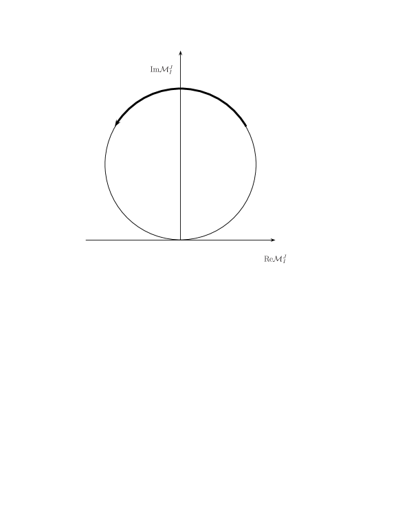
(a) Breit-Wigner; the amplitude is maximal at $s=m_{R}^{2}$.

(b) Resonance with background phase of about $\pi/2$. The amplitude is zero at $s=m_{R}^{2}$.

Figure 3.3: Resonances in an Argand diagram.

Such a resonance is called Breit-Wigner after the inventors of the formula for the cross section describing such a resonance. For the scattering amplitude we have in the Breit-Wigner case (dropping isospin labels) in the neighborhood of $m_{R}^{2}$, the mass of the resonance squared,

$$\mathcal{M}^{J}_{I}=\frac{\Gamma}{(m_{R}^{2}-s)-i\Gamma/2},$$ (3.118)

with $\Gamma$ the width of the resonance. The phase shift is then given by

$$\tan\delta=\frac{\Gamma/2}{m_{R}^{2}-s}.$$ (3.119)

If $s$ changes from values below $m_{R}^{2}$ to values above, $\delta$ changes rapidly from zero through $\pi/2$ to $\pi$ (or odd multiples thereof).

3.8.3 Background

In general resonances are as in the Breit-Wigner case characterized by the two parameters $\Gamma$ and $m_{R}$ and a rapid phase shift. However, these quantities are in general not directly related to the position and width of a peak in cross section. They rather denote the position of the pole of $\mathcal{M}$. Also the rapid phase shift does not necessarily occur at $\pi/2$ (or a multiple thereof). It may happen that the rapid phase shift begins only when the phase has already appreciable values different from zero.

Figure 3.4 shows four possibilities of a resonant phase shift and its corresponding characteristic behavior of the cross section.

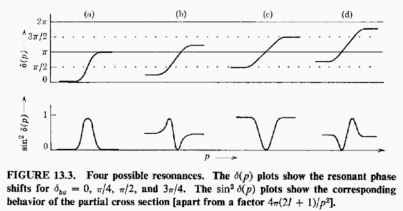
Figure 3.4: Phase shifts and corresponding characteristic feature of the cross section; from [28, p. 242].

Appreciable background phases are not just a mathematical possibility but seem to occur in actual physical reactions. One prominent example is the $f_{0}(980)$ which appears as a dip in the $\pi\pi$ spectrum because the corresponding phase shift increases rapidly through $\pi$ and not through $\pi/2$ as for a pure resonance. In the Argand diagram the amplitude moves rapidly through the bottom of the unitarity circle, see figure 3.3 (b). The experimental data and a parametrization of the relevant phase shift is shown in figure 3.5 together with the inelasticity. In figure 3.6 the cross-section of the isoscalar S wave is compiled. Such a structure can be explained by two rapid phase shifts through $\pi$ and $2\pi$, as I roughly simulated in figure 3.7.

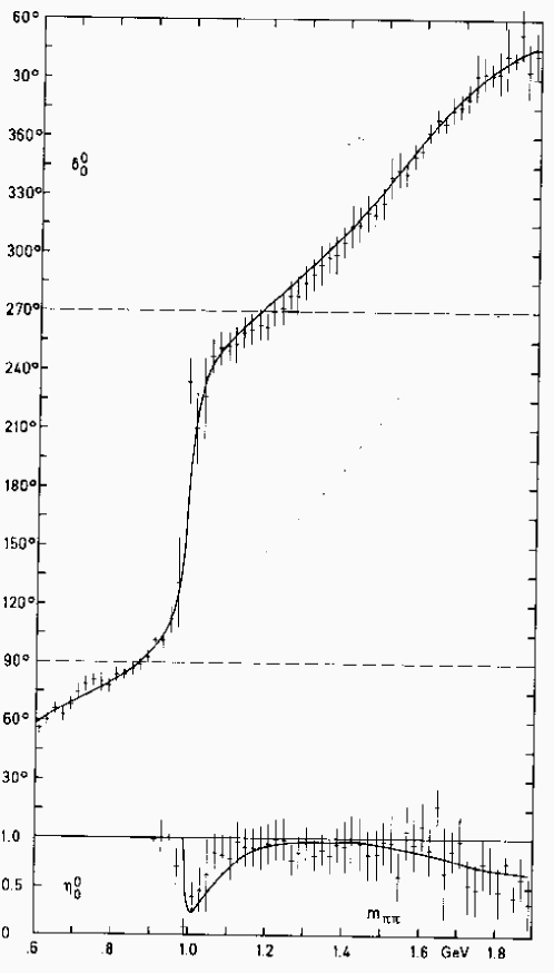
Figure 3.5: Resonant phase shift starting from an appreciable background phase in the isoscalar S wave. In the lower panel the behavior of the inelasticity in this partial wave is shown; from [29].

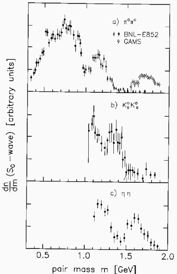
Figure 3.6: Compilation of the isoscalar S wave. Three major peaks or alternatively two major dips can be seen. Copied from [12], see references therein.

Figure 3.7: (a) Very rough parametrization of a phase shift that gives rise to a cross-section comparable to that of figure 3.6. (b) $\sin^{2}$ of the rough parametrization of the phase shift, which gives the characteristic form of the corresponding partial cross section.

3.9 Optical theorem

In the special case where the initial an the final state are the same, so-called forward scattering, the unitarity condition for the $T$ matrix (equation (3.96)) reads

$$\begin{split}i(T_{\alpha\alpha}^{*}-T_{\alpha\alpha})&=\int d\beta\,T^{\dagger}_{\alpha\beta}T_{\beta\alpha},\\ 2\text{Im}T_{\alpha\alpha}&=\int d\beta\,|T_{\beta\alpha}|^{2},\\ \text{Im}T_{\alpha\alpha}&=8\pi^{2}p\sqrt{s}\sigma_{\text{tot}}.\end{split}$$ (3.120)

To obtain a form of the optical theorem in terms of $\mathcal{M}$ we have to take care again about delta functions. Therefore, we cannot substitute simply $T=\delta^{4}(p_{i}-p_{f})\mathcal{M}$ in the above equation. In ref. [3, p. 147] this is done by dividing through delta function, which I want to avoid. The alternative that I prefer is again by means of wave-packets, cf. [27, p. 183ff]. I consider states of the form

$$|i\rangle=\sum_{m_{f}}\int d^{4}p_{i}\Phi^{(i)}(p_{i})|p_{i}\rangle\otimes|\psi_{i}\rangle.$$ (3.121)

Sandwiched between two such states $|i\rangle$ and $|f\rangle$ the operator equation (3.96) takes the form

$$\sum_{m_{f}}\int d^{4}p_{i}\Phi^{(i)}(p_{i})\Phi^{(f)*}(p_{i})(\mathcal{M}_{fi}-\mathcal{M}^{\dagger}_{fi})\\ =i\int d^{4}p_{i}\Phi^{(i)}(p_{i})\Phi^{(f)*}(p_{i})\sum_{m_{f}=2}^{M}\sum_{\Lambda}\int dQ_{m_{f}}\,\mathcal{M}^{\dagger}_{(f_{\Lambda})\psi}\mathcal{M}_{\psi_{i}}.$$ (3.122)

Since the momentum distribution functions $\Phi$ are arbitrary the integrands have to be equal. Therefore, by equation (3.39), we obtain for forward scattering, i. e. $i=f$,

$$\text{Im}\mathcal{M}_{ii}=8\pi^{2}p\sqrt{s}\sigma_{\text{tot}},$$ (3.123)

the right-hand side of which is the same as in equation (3.120), in this sense the delta-function relating $T$ and $\mathcal{M}$ has canceled. The result of equation (3.123) could have been found also by first showing that $\mathcal{M}$ satisfies the same form of unitarity condition as $T$, i. e.

$$i(\mathcal{M}^{\dagger}-\mathcal{M})=\mathcal{M}^{\dagger}\mathcal{M},$$ (3.124)

see, for instance [3, p. 147].

Because $\mathcal{M}$ and $T$ satisfy the same form of unitarity condition (equations (3.96) and (3.124)) I will often use $T$ and $\mathcal{M}$ interchangeable. In particular when discussing unitarity constraints (section 5.2.1) I will use $T$ elements without worrying much about the relation to the $\mathcal{M}$ elements in my conventions. None of the results obtained later hinge on the difference between $T$ and $\mathcal{M}$. Thus I adopt the notation of [11, 30] for formulating unitarity constraints.

3.10 Diffraction peak

The element of phase space of a two-body, i. e. $m_{f}=2$, final state is

$$dQ_{2}=\frac{d^{3}p_{1}}{2E_{1}}\frac{d^{3}p_{2}}{2E_{2}}\delta^{4}(p_{1}+p_{2}-p_{a}-p_{b}),$$ (3.125)

where $p_{1}$ and $p_{2}$ are the four-momenta of the two final state particles, and $p_{a}$ and $p_{b}$ the four-momenta of the two initial particles. We now discuss this expression in the center-of-mass frame where we have, by definition, that $\vec{p_{a}}+\vec{p_{b}}=0$. Thus, cf. [3, p. 139ff.],

$$dQ_{2}=\frac{d^{3}p_{1}}{2E_{1}}\frac{d^{3}p_{2}}{2E_{2}}\delta^{3}(\vec{p_{1}}+\vec{p_{2}})\delta(E_{1}+E_{2}-E_{a}-E_{b})\\ =\frac{1}{2\sqrt{m_{1}^{2}+\vec{p_{2}}^{2}}}\frac{d^{3}p_{2}}{2E_{2}}\delta(\sqrt{m_{1}^{2}+\vec{p_{2}}^{2}}+E_{2}-E_{a}-E_{b})\\ =\frac{1}{2\sqrt{m_{1}^{2}+\vec{p_{2}}^{2}}}\frac{|\vec{p_{2}}|^{2}d|\vec{p_{2}}|d\phi\,d\theta\,\sin\theta}{2\sqrt{m_{2}^{2}+\vec{p_{2}}^{2}}}\delta(\sqrt{m_{1}^{2}+\vec{p_{2}}^{2}}+\sqrt{m_{2}^{2}+\vec{p_{2}}^{2}}-E_{a}-E_{b}).$$ (3.126)

For the delta function we can use

$$\delta(f(|\vec{p_{2}}|))=\frac{\delta(|\vec{p_{2}}|-q)}{|f^{\prime}(q)|}$$ (3.127)

with $q$ the zero of $f(|\vec{p_{2}}|)$ and find

$$\delta(\sqrt{m_{1}^{2}+\vec{p_{2}}^{2}}+\sqrt{m_{2}^{2}+\vec{p_{2}}^{2}}-E_{a}-E_{b})\\ =\delta(|\vec{p_{2}}|-q)\frac{E_{1}E_{2}q}{(E_{a}+E_{b})},$$ (3.128)

with

$$q=\frac{\sqrt{[(E_{a}+E_{b})^{2}-m_{1}^{2}-m_{2}^{2}]^{2}-4m_{1}^{2}m_{2}^{2}}}{2(E_{a}+E_{b})}.$$ (3.129)

Thus we obtain the relation between the two-body phase space and the scattering angles $\theta$ and $\phi$ in the cms frame:

$$dQ_{2}=\frac{q}{4(E_{a}+E_{b})}d\phi\,d\theta\,\sin\theta\equiv\frac{q}{4(E_{a}+E_{b})}d\phi\,d(\cos\theta)\equiv\frac{q}{4(E_{a}+E_{b})}d\Omega.$$ (3.130)

We can now make an estimation that reveals a certain behavior of the total cross section for two-particle to two-body scattering, cf. equation (3.35). We assume that the matrix elements of $\mathcal{M}$ are smooth functions of the scattering solid angle $\Omega$ and that they fall off to zero for large angles. Then we can find a solid angle $\Delta\Omega$ such that

$$\int d\Omega\,|\mathcal{M}_{(f_{\Lambda})i}|^{2}\geq\frac{1}{2}\Delta\Omega|\mathcal{M}_{ii}|^{2}.$$ (3.131)

Then we obtain

$$\sigma_{\text{tot}}\geq\sigma_{\Lambda}(2\to 2)=\frac{1}{16\pi^{2}p\sqrt{s}}\int dQ_{m_{f}}\,|\mathcal{M}_{(f_{\Lambda})i}|^{2}\\ =\frac{1}{16\pi^{2}p\sqrt{s}}\frac{q}{4(E_{a}+E_{b})}\int d\Omega\,|\mathcal{M}_{(f_{\Lambda})i}|^{2}\\ \geq\frac{1}{16\pi^{2}p\sqrt{s}}\frac{q}{4(E_{a}+E_{b})}\Delta\Omega|\mathcal{M}_{ii}|^{2}\\ \geq\frac{1}{16\pi^{2}p\sqrt{s}}\frac{q}{4(E_{a}+E_{b})}\Delta\Omega|\text{Im}\mathcal{M}_{ii}|^{2}\\ =\frac{1}{16\pi^{2}p\sqrt{s}}\frac{q}{4(E_{a}+E_{b})}\Delta\Omega 64\pi^{4}p^{2}s\sigma^{2}_{\text{tot}}.$$ (3.132)

In the cms $p=q$, $E_{a}+E_{b}=\sqrt{s}$. So we obtain an upper bound for $\Delta\Omega$,

$$\Delta\Omega\leq\frac{1}{\pi^{2}p^{2}\sigma_{\text{tot}}}.$$ (3.133)

Hadronic cross sections show a diffraction peak, i. e. the differential cross section falls off exponentially with $t=2p^{2}(\cos\theta-1)$ (cf. eq. (3.82)). In the special case of a totally absorbing disk of radius $R$ (see e. g. [31, p. 136f.] and [27, p. 210f.]) we have approximately

$$\frac{d\sigma}{dt}\propto\exp\left(-\frac{R^{2}|t|}{4}\right).$$ (3.134)

In figure 3.8 the differential cross section for elastic proton-proton scattering is shown. There we see that already for incident momenta of 5 GeV (i. e. $\sqrt{s}\approx 3.4\ \text{GeV}$) the fall-off is visible but that the diffraction peak is more and more pronounced for higher incident momenta (in the figure up to 1480 GeV, i. e. $\sqrt{s}\approx 53\ \text{GeV}$).

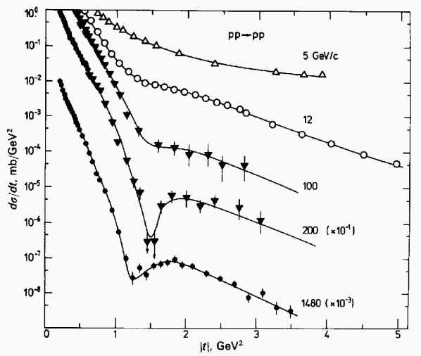
Figure 3.8: Differential cross section for elastic $pp$ scattering as a function of the square of the momentum transfer, $|t|$; from [31, p. 137].

As shown in figure 3.9, typical hadronic cross sections rise with energies for energies greater than roughly 20 GeV. Thus also equation (3.133) shows that the forward peak in the two-body to two-body total hadronic cross section becomes more and more narrow at these high energies.

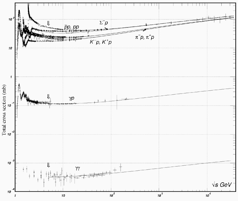
Figure 3.9: High energy behavior of typical hadronic cross sections; from [14].

Chapter 4 Kinematics of a three body decay

In this chapter I collect kinematical relations that could eventually be used for a partial wave analysis. As a numeric example I take the decay $B^{+}\to\pi^{-}\pi^{+}K^{+}$.

4.1 Rest system of decaying particle

First I consider the kinematical relations that hold in the rest system of the $B$ meson. By definition its three momentum is zero, $\vec{p}_{B}=0$, in this frame of reference. Its energy is given by its mass $m_{B}$. The squares of the respective two-body invariant masses are defined by

$$\begin{split}s_{\pi^{-}\pi^{+}}&=(p_{\pi^{-}}+p_{\pi^{+}})^{2}=(E_{\pi^{-}}+E_{\pi^{+}})^{2}-(\vec{p}_{\pi^{-}}+\vec{p}_{\pi^{+}})^{2},\\ s_{\pi^{-}K^{+}}&=(p_{\pi^{-}}+p_{K^{+}})^{2}=(E_{\pi^{-}}+E_{K^{+}})^{2}-(\vec{p}_{\pi^{-}}+\vec{p}_{K^{+}})^{2},\\ s_{\pi^{+}K^{+}}&=(p_{\pi^{+}}+p_{K^{+}})^{2}=(E_{\pi^{+}}+E_{K^{+}})^{2}-(\vec{p}_{\pi^{+}}+\vec{p}_{K^{+}})^{2}.\end{split}$$ (4.1)

Recall that these quantities are Lorentz invariant; the energies and the three-momenta for one particle pair can be taken with respect to any reference frame. (But it has to be the same reference frame for the energy and the three-momentum.) For the sake of brevity I will sometimes refer to these quantities just as “two-body masses”, “pair masses” or the like. These masses (squared) of one pair of particles are related to the energy of the remaining particle, e. g.

$$\begin{split}s_{\pi^{-}\pi^{+}}&=(E_{\pi^{-}}+E_{\pi^{+}})^{2}-(\vec{p}_{\pi^{-}}+\vec{p}_{\pi^{+}})^{2}\\ &=(m_{B}-E_{K^{+}})^{2}-\vec{p}_{K^{+}}^{2}\\ &=m_{B}^{2}+m_{K^{+}}^{2}-2m_{B}E_{K^{+}},\end{split}$$ (4.2)

and therefore also to the modulus of the three-momentum of the remaining particle:

$$\begin{split}\vec{p}_{K^{+}}^{2}&=E_{K^{+}}^{2}-m_{K^{+}}^{2}\\ &=\left(\frac{m_{B}^{2}+m_{K^{+}}^{2}-s_{\pi^{-}\pi^{+}}}{2m_{B}}\right)^{2}-m_{K^{+}}^{2}\\ &=\frac{m_{B}^{4}+m_{K^{+}}^{4}+s_{\pi^{-}\pi^{+}}^{2}-2(m_{B}^{2}m_{K^{+}}^{2}+m_{B}^{2}s_{\pi^{-}\pi^{+}}+m_{K^{+}}^{2}s_{\pi^{-}\pi^{+}})}{4m_{B}^{2}}.\end{split}$$ (4.3)

Similarly, one obtains expressions for $E_{\pi^{-}}$ and $\vec{p}_{\pi^{-}}^{2}$, and $E_{\pi^{+}}$ and $\vec{p}_{\pi^{+}}^{2}$ in terms of $s_{\pi^{+}K^{+}}$ and $s_{\pi^{-}K^{+}}$ respectively, see table 4.1.

4.2 Two-body system

We now make a Lorentz transformation into the center-of-mass system (cms) of the two pions, say. The kinematic situation in this reference system is shown in figure 4.1. Compare it to the kinematic situation in scattering in the cms shown in figure 4.2.

Figure 4.1: Kinematic situation for the three-body decay $B^{+}\to\pi^{-}\pi^{+}K^{+}$ in the $\pi\pi$ rest system with the two-body angle $\theta$ as defined in equation (4.13), $z\equiv\cos\theta$. Top of the figure: before the decay of the $B$. Bottom of the figure: after the decay and the strong final state interactions.

Figure 4.2: Kinematic situation for scattering in the center-of-mass system. Top of the figure: before the strong interactions. Bottom of the figure: after the strong interactions.

The appropriate transformation from the $B$ rest system to the $\pi\pi$ system is a Lorentz boost along the direction opposite to $\vec{p}_{K^{+}}$. The relative velocity between the $B$ rest system and the two-body system considered now is (in unities of $c$ and with respect to the direction of $\vec{p}_{K^{+}}$)

$$v=-\frac{|\vec{p}_{\pi^{-}}+\vec{p}_{\pi^{+}}|}{E_{\pi^{-}}+E_{\pi^{+}}}=-\frac{|\vec{p}_{K^{+}}|}{m_{B}-E_{K^{+}}}.$$ (4.4)

This velocity defines the hyperbolic angle $\alpha$ by which a Lorentz boost along a given axis (here the axis given by $\vec{p}_{K^{+}}$) can be specified: $\tanh\alpha=v$. The matrix that represents the Lorentz boost then reads

$$\begin{pmatrix}\cosh\alpha&-\sinh\alpha&0&0\\ -\sinh\alpha&\cosh\alpha&0&0\\ 0&0&1&0\\ 0&0&0&1\end{pmatrix}.$$ (4.5)

Accordingly, the energy of the $B$ in the new reference frame is

$$\begin{split}E_{B}^{\prime}=m_{B}\cosh\alpha&=m_{B}\frac{m_{B}-E_{K^{+}}}{\sqrt{s_{\pi^{-}\pi^{+}}}}\\ &=\frac{m_{B}}{\sqrt{s_{\pi^{-}\pi^{+}}}}\left(m_{B}-\frac{m_{B}^{2}+m_{K^{+}}^{2}-s_{\pi^{-}\pi^{+}}}{2m_{B}}\right)\\ &=\frac{m_{B}^{2}-m_{K^{+}}^{2}+s_{\pi^{-}\pi^{+}}}{2\sqrt{s_{\pi^{-}\pi^{+}}}}.\end{split}$$ (4.6)

In the center-of-mass system of the two pions we have $E_{B}^{\prime}=\sqrt{s_{\pi^{-}\pi^{+}}}+E_{K^{+}}^{\prime}$. The energy of the $K^{+}$ in this system is therefore given by

$$E_{K^{+}}^{\prime}=E_{B}^{\prime}-\sqrt{s_{\pi^{-}\pi^{+}}}=\frac{m_{B}^{2}-m_{K^{+}}^{2}-s_{\pi^{-}\pi^{+}}}{2\sqrt{s_{\pi^{-}\pi^{+}}}}.$$ (4.7)

By definition of this reference frame the three-momenta of the two pions are equal, $\vec{p}_{\pi^{-}}^{\prime}=\vec{p}_{\pi^{+}}^{\prime}$. So are, by momentum conservation, the three-momenta of the $B$ and the $K$, $\vec{p}_{B}^{\prime}=\vec{p}_{K^{+}}^{\prime}$. I denote the respective moduli of the three-momenta of the pions and the $B$ (or $K$) as $k$ and $l$. $l$ is determined by energy conservation in the new reference frame,

$$\sqrt{m_{B}^{2}+l^{2}}=\sqrt{m_{K^{+}}+l^{2}}+\sqrt{s_{\pi^{-}\pi^{+}}},$$ (4.8)

which equation can be solved for $l$, yielding

$$l^{2}=\frac{m_{B}^{4}+m_{K^{+}}^{4}+s_{\pi^{-}\pi^{+}}^{2}-2(m_{B}^{2}m_{K^{+}}^{2}+m_{B}^{2}s_{\pi^{-}\pi^{+}}+m_{K^{+}}^{2}s_{\pi^{-}\pi^{+}})}{4s_{\pi^{-}\pi^{+}}}.$$ (4.9)

As to the three-momentum $k$ of the pions, it can be obtained by evaluating the Lorentz invariant quantity $s_{\pi^{-}\pi^{+}}$ in the new reference system, i. e.

$$\sqrt{s_{\pi^{-}\pi^{+}}}=\sqrt{m_{\pi^{-}}^{2}+k^{2}}+\sqrt{m_{\pi^{+}}^{2}+k^{2}},$$ (4.10)

which upon solving yields

$$k^{2}=\frac{m_{\pi^{-}}^{4}+m_{\pi^{+}}^{4}+s_{\pi^{-}\pi^{+}}^{2}-2(m_{\pi^{-}}^{2}m_{\pi^{+}}^{2}+m_{\pi^{-}}^{2}s_{\pi^{-}\pi^{+}}+m_{\pi^{+}}^{2}s_{\pi^{-}\pi^{+}})}{4s_{\pi^{-}\pi^{+}}}.$$ (4.11)

The respective energies of the pions in the primed reference system are then

$$E_{\pi^{-}}^{\prime}=\sqrt{m_{\pi^{-}}^{2}+k^{2}},\qquad E_{\pi^{+}}^{\prime}=\sqrt{m_{\pi^{+}}^{2}+k^{2}}.$$ (4.12)

One relevant quantity for a partial-wave analysis is the angle $\theta$ between the respective directions of the $\pi^{-}$ and the $K^{+}$ in the new reference frame, i. e. the center-of-mass system of the two pions. We are now going to derive an expression for the cosine of this angle, i. e. $z=\cos\theta$, in terms of the two variables of the Dalitz plot, $s_{\pi^{-}\pi^{+}}$ and $s_{\pi^{-}K^{+}}$, and the masses of the four particles concerned. By definition we have

$$z=\frac{\vec{p}_{\pi^{-}}^{\prime}\vec{p}_{K^{+}}^{\prime}}{|\vec{p}_{\pi^{-}}^{\prime}||\vec{p}_{K^{+}}^{\prime}|}=\frac{-p_{\pi^{-}}p_{K^{+}}+E_{\pi^{-}}^{\prime}E_{K^{+}}^{\prime}}{kl}.$$ (4.13)

Suitable expressions for $E_{\pi^{-}}^{\prime}$, $E_{K^{+}}^{\prime}$, $k$ and $l$ are given, respectively, in the equations (4.12), (4.7), (4.11) and (4.9). For $p_{\pi^{-}}p_{K^{+}}$ we have

$$p_{\pi^{-}}p_{K^{+}}=E_{\pi^{-}}E_{K^{+}}-\vec{p}_{\pi^{-}}\vec{p}_{K^{+}}.$$ (4.14)

For $E_{K^{+}}$ we have already derived a relation between it and the Dalitz plot variable $s_{\pi^{-}\pi^{+}}$ (equation (4.2)). The scalar product between the two three-momenta can be expressed by the moduli squared of the three-momenta of all three decay products, by transforming the relation for momentum conservation first by putting it in an appropriate form then squaring it and finally solving it for $\vec{p}_{\pi^{-}}\vec{p}_{K^{+}}$:

$$\begin{split}\vec{p}_{\pi^{-}}+\vec{p}_{K^{+}}+\vec{p}_{\pi^{+}}&=\vec{p}_{B}=0,\\ \vec{p}_{\pi^{-}}+\vec{p}_{K^{+}}&=-\vec{p}_{\pi^{+}},\\ \vec{p}_{\pi^{-}}^{2}+\vec{p}_{K^{+}}^{2}+2\vec{p}_{\pi^{-}}\vec{p}_{K^{+}}&=\vec{p}_{\pi^{+}}^{2},\\ \vec{p}_{\pi^{-}}\vec{p}_{K^{+}}&=\frac{\vec{p}_{\pi^{+}}^{2}-\vec{p}_{\pi^{-}}^{2}-\vec{p}_{K^{+}}^{2}}{2}.\end{split}$$ (4.15)

The squares of three momenta in terms of the three two-body masses are given by equation (4.3) and the respective entries in table 4.1. To express all quantities in the two Dalitz plot variables $s_{\pi^{-}\pi^{+}}$ and $s_{\pi^{-}K^{+}}$, it remains to find an expression for $s_{\pi^{+}K^{+}}$ in terms of these. Such an expression can be obtained as follows.

$$s_{\pi^{-}\pi^{+}}+s_{\pi^{-}K^{+}}+s_{\pi^{+}K^{+}}=(p_{\pi^{-}}+p_{\pi^{+}})^{2}+(p_{\pi^{-}}+p_{K^{+}})^{2}+(p_{\pi^{+}}+p_{K^{+}})^{2}\\ =p_{\pi^{-}}^{2}+p_{\pi^{+}}^{2}+p_{K^{+}}^{2}\\ +p_{\pi^{-}}^{2}+p_{\pi^{+}}^{2}+p_{K^{+}}^{2}+2(p_{\pi^{-}}p_{\pi^{+}}+p_{\pi^{-}}p_{K^{+}}+p_{\pi^{+}}p_{K^{+}}).$$ (4.16)

Because of energy-momentum conservation we have

$$\begin{split}m_{B}^{2}=p_{B}^{2}&=(p_{\pi^{-}}+p_{\pi^{+}}+p_{K^{+}})^{2}\\ &=p_{\pi^{-}}^{2}+p_{\pi^{+}}^{2}+p_{K^{+}}^{2}+2(p_{\pi^{-}}p_{\pi^{+}}+p_{\pi^{-}}p_{K^{+}}+p_{\pi^{+}}p_{K^{+}}).\end{split}$$ (4.17)

Using this result and since $p_{\pi^{-}}^{2}=m_{\pi^{-}}^{2}$ etc., equation (4.16) reads

$$s_{\pi^{-}\pi^{+}}+s_{\pi^{-}K^{+}}+s_{\pi^{+}K^{+}}=m_{\pi^{-}}^{2}+m_{\pi^{+}}^{2}+m_{K^{+}}^{2}+m_{B}^{2}.$$ (4.18)

So to obtain expressions in the two Dalitz plot variables $s_{\pi^{-}\pi^{+}}$ and $s_{\pi^{-}K^{+}}$ one can replace every occurrence of $s_{\pi^{+}K^{+}}$ by $m_{B}^{2}+m_{\pi^{-}}^{2}+m_{\pi^{+}}^{2}+m_{K^{+}}^{2}-s_{\pi^{-}\pi^{+}}-s_{\pi^{-}K^{+}}$.

The corresponding formulae for the other two two-body systems, i. e. the cms of the negative or positive pion and the kaon, can be obtained by making appropriate substitutions. In the case considered so far, i. e. the cms of the two pions, the kaon played the role of the spectator, the negative pion the role of the particle with respect to which the angle $\theta$ is measured. In the cms of the negative pion and the kaon, the positive pion is the spectator, the reference particle for the angle I take to be the negative pion. (It could equally well be the kaon, this is just my convention. With the kaon as reference for the angle, $z$ would change sign.) In the cms of the positive pion and the kaon, the negative pion is the spectator and the kaon (or the positive pion) is the reference particle for the angle.

Table 4.1: Expressions for energies, three-momenta and cosine of the scattering angle in the $B$ rest system (2nd column), the center-of-mass system of the two pions (3rd column), the center-of-mass system of the negative pion and the kaon (4th column), and the center-of-mass system of the positive pion and the kaon (5th column). $\lambda(a,b,c)=a^{2}+b^{2}+c^{2}-2(ab+ac+bc)$.

4.3 Pair masses and two-body angles

4.3.1 Resonance band or angular peak?

In a typical Dalitz plot for $B^{+}\to\pi^{-}\pi^{+}K^{+}$ each decay event is assigned a coordinate pair $(s_{\pi^{-}\pi^{+}},s_{\pi^{-}K^{+}})$. With the kinematic constraints discussed in this chapter the decay events can be identified equivalently by other pairs of kinematic quantities. For the task of identifying resonance masses and spins one is interested in the invariant pair masses $s_{\pi^{-}\pi^{+}}$, $s_{\pi^{-}K^{+}}$ and $s_{K^{+}\pi^{+}}$, and in the two-body angles $\theta_{\pi^{-}\pi^{+}}$, $\theta_{\pi^{-}K^{+}}$ and $\theta_{K^{+}\pi^{+}}$. In figures 4.3 to 4.8 lines of constant $s$ and $z\equiv\cos\theta$ are drawn using the Maple command implicitplot. With any two out of these six patterns one can construct one of ${6\choose 2}=15$ coordinate systems for the three-body decay events.

The possibility of using coordinate systems consisting of angles and pair masses shows that the interpretation of structures in the Dalitz plot event distribution like bands (see figures 2.1 and 2.2) is a priori not unique. A concentration of events in a certain region of the Dalitz plot can obtain because certain pair masses are more likely to be produced in the decay or because certain angular distributions in a two-body subsystem are preferred.

Figure 4.3: Lines where $s_{\pi^{-}\pi^{+}}=(5,10,15,20,25)\,\text{GeV}^{2}$. Abscissa: $s_{\pi^{-}\pi^{+}}\ [\text{GeV}^{2}]$. Ordinate: $s_{\pi^{-}K^{+}}\ [\text{GeV}^{2}]$.

Figure 4.4: Lines where $s_{\pi^{-}K^{+}}=(5,10,15,20,25)\,\text{GeV}^{2}$. Abscissa: $s_{\pi^{-}\pi^{+}}\ [\text{GeV}^{2}]$. Ordinate: $s_{\pi^{-}K^{+}}\ [\text{GeV}^{2}]$.

Figure 4.5: Lines where $s_{K^{+}\pi^{+}}=(0,5,10,15,20,25)\,\text{GeV}^{2}$.

Figure 4.6: Lines where $z_{\pi^{-}\pi^{+}}=\pm 1,\pm 0.8,\pm 0.6,\pm 0.4,\pm 0.2,\pm 0.1$. Abscissa: $s_{\pi^{-}\pi^{+}}\ [\text{GeV}^{2}]$. Ordinate: $s_{\pi^{-}K^{+}}\ [\text{GeV}^{2}]$.

Figure 4.7: Lines where $z_{\pi^{-}K^{+}}=\pm 1,\pm 0.8,\pm 0.6,\pm 0.4,\pm 0.2,\pm 0.1$. Abscissa: $s_{\pi^{-}\pi^{+}}\ [\text{GeV}^{2}]$. Ordinate: $s_{\pi^{-}K^{+}}\ [\text{GeV}^{2}]$.

Figure 4.8: Lines where $z_{K^{+}\pi^{+}}=\pm 1,\pm 0.8,\pm 0.6,\pm 0.4,\pm 0.2,\pm 0.1$. Abscissa: $s_{\pi^{-}\pi^{+}}\ [\text{GeV}^{2}]$. Ordinate: $s_{\pi^{-}K^{+}}\ [\text{GeV}^{2}]$.

4.3.2 Partial waves

The coordinate lines of the two-body angle can eventually be used for a partial wave analysis. In the decay $B^{+}\to\pi^{-}\pi^{+}K^{+}$ the line of constant $z_{\pi^{-}K^{+}}=0$ could be of particular importance. In [8] the reference amplitude and phase is taken to be the signal from

$$B^{+}\to K^{*}(892)\pi^{+}\to K^{+}\pi^{-}\pi^{+}.$$ (4.19)

$K^{*}(892)$ has spin $J=1$ and should thus show its particular angular dependence given by the Legendre polynom

$$P_{1}(z_{\pi^{-}K^{+}})=z_{\pi^{-}K^{+}}\equiv\cos\theta_{\pi^{-}K^{+}}.$$ (4.20)

The partial wave amplitude representing a decay via the $K^{*}(892)$ is therefore expected to vanish where $z_{\pi^{-}K^{+}}=0$.

In figure 4.9 the three lines $z_{\pi^{-}\pi^{+}}=0$, $z_{\pi^{-}K^{+}}=0$, $z_{\pi^{+}K^{+}}=0$ are plotted.

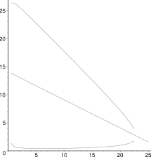
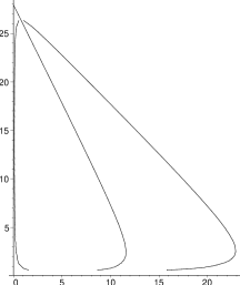
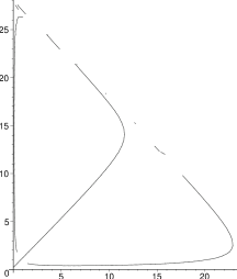
Figure 4.9: Lines with (a) $z_{\pi^{-}\pi^{+}}=0$, (b) $z_{\pi^{-}K^{+}}=0$, (c) $z_{\pi^{+}K^{+}}=0$ and parts of the Dalitz-plot boundary, i. e. with $|z|=1$ for the respective $z$’s. Abscissa: $s_{\pi^{-}\pi^{+}}\ [\text{GeV}^{2}]$. Ordinate: $s_{\pi^{-}K^{+}}\ [\text{GeV}^{2}]$.

Chapter 5 Guidelines for Dalitz plot analysis

5.1 Surrogate scattering laboratories

Experimentally, collisions with an unstable target (and beam) particle like $\pi\pi\to\pi\pi$ and $K\pi\to K\pi$ are not feasible. Chew and Low [13] proposed that one can study such reactions in scattering of the beam particle off a stable target whereby the beam particle actually scatters with a virtual particle that is exchanged between the beam and the target particle. Two typical reactions of this type which serve as surrogate laboratory for scattering of unstable particles are $\pi^{-}p\to\pi^{-}\pi^{+}n$ and $K^{-}p\to K^{-}\pi^{+}n$, see also section 5.2.3. Another possibility in a similar vein is to study e. g. the scattering of two pions in the final state of a three-body decay such as $J/\psi\to\phi\pi\pi$ where as a good approximation the $\phi$ can be assumed not to interact with the pions [11, p. 1188, p. 1193]. As a by-product of the extensive CP-violation studies in $B$ decays like $B^{+}\to K^{+}\pi^{+}\pi^{-}$ there is now a lot of new data available from a similar type of surrogate laboratory for final-state scattering of pions and kaons. One great advantage of using this new data is the huge amount of events such that it should be possible to interpret structures of the corresponding Dalitz plots that in earlier Dalitz plots would not be distinguishable from statistical fluctuations or not visible at all.

Another feature of the reaction $B^{+}\to K^{+}\pi^{+}\pi^{-}$ is that contrary to the case of $J/\psi\to\phi\pi\pi$ the approximation that only two of the three final state particles interact is not applicable. Rather the pairwise interactions between all three final state particles are of the same order in strength. However, as an approximation one can assume that the interactions can be regarded as a superposition of three pairwise interactions and neglect the simultaneous interaction of all three particles in the final state, see equation (5.1).

I will propose some guidelines for a Dalitz plot analysis for the three-body decay $B^{+}\to K^{+}\pi^{+}\pi^{-}$. I concentrate on this example because it allows to show that an analysis in terms of a sum of Breit-Wigner terms and a non-resonant contribution à la Belle and Babar [16, 8, 26] may be at odds with what is known about the involved two-body systems and insufficient to extract new or confirm old information about those.

The goal of investigating the strong interactions of the final state particles of the three-body decay defines a region of interest in the Dalitz plot. Controversial issues in the hadron spectroscopy of pions and kaons include the $\sigma$, the $\kappa$, the $f_{0}(980)$, the $f_{0}(1370)$, the $f_{0}(1500)$ and the $K^{*}(1430)$. These are structures in the $\pi\pi$ and $K\pi$ mass-region from zero to about 1500 MeV. These mass intervals corresponds to the lower left corner of the Dalitz plot of $B^{+}\to K^{+}\pi^{+}\pi^{-}$ in the usual representations of e. g. Belle.

5.2 Three-body decay and two-body amplitudes

As an approximation one can think of a three-body decay like $B^{+}\to\pi^{-}\pi^{+}K^{+}$ as the superposition of three amplitudes for the production of a two-body state with an accompanying spectator, i. e. a particle which apart from its mere presence does not make any difference for the interactions taking place,

$$T(B^{+}\to\pi^{-}\pi^{+}K^{+})=T(B^{+}\to(\pi^{-}\pi^{+})K^{+})+T(B^{+}\to(\pi^{-}K^{+})\pi^{+})\\ +T(B^{+}\to\pi^{-}(\pi^{+}K^{+})).$$ (5.1)

Each of the production amplitudes on the right-hand side can be related to the scattering amplitude of the respective two-body system. The relation that I will give is distinguished by that it is by construction consistent with unitarity constraints as discussed in the following, cf. [11, 30].

Here and in the following I use with refs. [11, 30] $T$ elements for discussing unitarity constraints. In my conventions the relevant quantity would rather be $\mathcal{M}$. $\mathcal{M}$ and $T$ do, however, satisfy the same form of unitarity constraint, see equations (3.96) and (3.124). Therefore, the difference between $T$ and $\mathcal{M}$ is irrelevant here.

5.2.1 Unitarity and production amplitudes

To see how the production amplitudes of the right-hand side of equation (5.1) relates to the respective two-body scattering amplitudes, let us take as an example the amplitude $T(B^{+}\to\pi^{-}(\pi^{+}K^{+}))$. The unitarity constraint takes into consideration the channels $B^{+}$, $\pi^{-}(\pi^{+}K^{+})$ and inelastic channels of the scattering of $\pi^{+}K^{+}$ (with $\pi^{-}$ as spectator) like $\pi^{-}(\pi^{+}K^{+}\pi^{-}\pi^{+})$. I enumerate the channels as

$$1=B^{+},\qquad 2=\pi^{-}(\pi^{+}K^{+}),\qquad 3=\pi^{-}(\pi^{+}K^{+}\pi^{-}\pi^{+}),\quad\dots,$$ (5.2)

where the dots stand for the prescription to enumerate all further inelastic $\pi^{+}K^{+}$-scattering channels. (There are no other channels with only two-particles to which $\pi^{+}K^{+}$ couples; no other two-particle state has the same quantum numbers as $\pi^{+}K^{+}$.)

I use the unitarity constraint $T^{\dagger}T=i(T^{\dagger}-T)$ in the form

$$\text{Im}T_{ji}=\frac{1}{2}\sum_{k}T^{*}_{jk}T_{ki}.$$ (5.3)

This means that I assume that the states can be properly discretized (cf. section 3.2.1) and that time reversal invariance is given, which I take to imply that the $T$ matrix is symmetric, in other words

$$T^{\dagger}=T^{*}.$$ (5.4)

The $B^{+}$ meson consists of an up- and an anti-bottom quark. It has thus bottomness 1. Strong interactions conserve the flavors. Therefore, since the $B$-meson is the lightest state with bottomness 1 it can only decay by electro-weak interactions. The elements $T_{1k}$ ($k\neq 1$) representing a transition from channel 1 (the $B^{+}$) to some other channel are therefore of order of magnitude of the electro-weak coupling constants, which in the energy region to be discussed here are small compared to the coupling constant of the strong interaction. In the following formulation of unitarity constraints I will neglect all terms quadratic in electro-weak couplings. To keep track of the different orders of magnitude of the electro-weak couplings I use a superscript ‘$w$’ for electro-weak amplitudes and a superscript ‘$s$’ for strong amplitudes.

The $S$ element for interactions in channel 1 and transitions from channel 1 to any other channel is purely weak,

$$S_{1i}=S_{1i}^{w},\quad i\in\{1,2,3,\dots\}.$$ (5.5)

On the other hand, interactions in and transitions between channels 2, 3, … are described by a Hamiltonian that is a sum of an electro-weak and a strong Hamiltonian,

$$H_{lm}=H_{lm}^{s}+H_{lm}^{w},\quad l,m\in\{2,3,\ldots\}.$$ (5.6)

The corresponding $S$ operator is therefore to leading order in $H_{lm}^{w}$ given by (see [32, p. 108]).

$$S=\lim_{t\to\infty}\exp(-iH_{lm}(2t))\approx\lim_{t\to\infty}(\mathbbm{1}-iH_{lm}^{w}t)\exp(-iH_{lm}^{s}(2t)).$$ (5.7)

For the $T_{lm}$ ($l,m\in\{2,3,\ldots\}$) elements we obtain

$$T_{lm}=-i(S_{lm}-\delta_{lm})\approx\lim_{t\to\infty}-i[(\delta_{lm}-iH_{lm}^{w}(2t))(\delta_{lm}+iT_{lm}^{s})-\delta_{lm}]\\ =T_{lm}^{s}S_{lm}^{w}+T_{lm}^{w},$$ (5.8)

with

$$T_{lm}^{w}=\lim_{t\to\infty}(-H_{lm}^{w}(2t))\quad\text{and}\quad S_{lm}^{w}=\lim_{t\to\infty}\exp(-iH_{lm}^{w}(2t)).$$ (5.9)

The factor $S^{w}$ gives a weak phase to the strong amplitude. This phase can be neglected in the present context as an overall phase. It can be absorbed by a redefinition of the state vectors. Not keeping track of this overall phase and neglecting quadratic and higher order terms of the weak $T$ elements we then have in and between channels 2, 3, …

$$T_{ji}=T_{ji}^{w}+T_{ji}^{s},\quad j,i\in\{2,3,\ldots\}.$$ (5.10)

The unitarity condition for the production amplitudes, $T^{w}_{1k}$ ($k\neq 1$), reads

$$2\text{Im}T^{w}_{1k} =\sum_{r=1}^{\dots}T^{*}_{1r}T_{rk}$$ (5.11)

$$=T^{w*}_{11}T^{w}_{1k}+\sum_{r=2}^{\dots}T^{w*}_{1r}(T^{s}_{rk}+T^{w}_{rk})$$ (5.12)

$$=\sum_{r=2}^{\dots}T^{w*}_{1r}T^{s}_{rk},$$ (5.13)

where in the last step terms quadratic in the weak coupling have again been dropped.

If the production amplitudes are written as,

$$T_{1k}=T^{w}_{1k}=\sum_{n=2}^{\dots}\alpha_{n}T_{nk}^{s},\quad k\neq 1,$$ (5.14)

where, importantly, the $\alpha$’s are real, the constraint of equation (5.13) is satisfied by construction; provided that the strong amplitudes $T_{nk}^{s}$ satisfy the unitartity condition among themselves, i. e.

$$2\text{Im}T^{s}_{lm}=\sum_{k}T^{s*}_{lk}T^{s}_{km},\quad k,l,m\in\{2,3,\ldots\}.$$ (5.15)

Indeed we then have:

$$2\text{Im}T^{w}_{1k}=2\text{Im}\sum_{n=2}^{\dots}\alpha_{n}T_{nk}^{s}=\sum_{n=2}^{\dots}\alpha_{n}2\text{Im}T_{nk}^{s}=\sum_{n=2}^{\dots}\alpha_{n}\sum_{r=2}^{\dots}T^{s*}_{nr}T^{s}_{rk}\\ =\sum_{r=2}^{\dots}\sum_{n=2}^{\dots}\alpha_{n}T^{s*}_{nr}T^{s}_{rk}=\sum_{r=2}^{\dots}T^{w*}_{1r}T^{s}_{rk}.$$ (5.16)

5.2.2 Elastic region for $\boldsymbol{\pi^{-}\pi^{+}}$ and $\boldsymbol{\pi^{-}K^{+}}$

Because of equation (4.16) not all three two-body cms energies can be low. The region of the Dalitz plot we are interested in is e. g. characterized by low values of $s_{\pi^{-}\pi^{+}}$ and $s_{\pi^{-}K^{+}}$ and high values of $s_{\pi^{+}K^{+}}$, roughly

$$0\ \text{GeV} \leq\sqrt{s_{\pi^{-}\pi^{+}}}\leq 1.6\ \text{GeV},$$ (5.17)

$$0\ \text{GeV} \leq\sqrt{s_{\pi^{-}K^{+}}}\leq 1.6\ \text{GeV},$$ (5.18)

$$3\ \text{GeV} \leq\sqrt{s_{\pi^{+}K^{+}}}\leq 5\ \text{GeV}.$$ (5.19)

From analyses of $\pi\pi$ scattering (e. g. CERN-Munich [29], see figure 3.5, lower panel) it is known that indeed the inelasticity is almost 1 up to 1.5 GeV, except for a small energy region around 980 MeV. This dip in the inelasticity may be due to the decay of $f_{0}(980)$ into $\pi\pi$ as well as into $K\bar{K}$. I neglect this inelasticity in the hope that the resulting ansatz is while simpler still able to represent the most relevant features of the process.

For the production amplitudes $T(B^{+}\to(\pi^{-}\pi^{+})K^{+})$ and $T(B^{+}\to(\pi^{-}K^{+})\pi^{+})$ we can therefore use an elastic unitarity condition that takes only elastic strong amplitudes to be non-zero. The respective production amplitudes have then the simple form $T_{1k}=T^{w}_{1k}=\alpha_{k}T_{kk}^{s}$, i. e.

$$\begin{split}T(B^{+}\to(\pi^{-}\pi^{+})K^{+})&=\alpha_{\pi^{-}\pi^{+}}T^{s}(\pi^{-}\pi^{+}\to\pi^{-}\pi^{+})\\ T(B^{+}\to(\pi^{-}K^{+})\pi^{+})&=\alpha_{\pi^{-}K^{+}}T^{s}(\pi^{-}K^{+}\to\pi^{-}K^{+}).\end{split}$$ (5.20)

This form of the production amplitude shows that, since $\alpha_{k}$ is real, the production amplitude and the strong amplitude of the interaction of the final state particles have the same phase. This result is known as Watson’s theorem, final state interaction theorem or just elastic unitarity. The name “final state interaction theorem” is justified by that the particular form of the production amplitude (eq. (5.14)), which is a solution for the unitarity constraint can be interpreted to the effect that the decay from channel 1 into a channel $k\neq 1$ is a sum of amplitudes representing the decay from channel 1 into channel $n\neq 1$ with coupling strength $\alpha$ followed by a strong final state interaction represented by $T_{nk}^{s}$ [11, 30]. In the original Watson theorem [15] it is explicitly two potentials that are considered: The potential responsible for the production of the hadrons, and the potential of the interaction of these hadrons in the final state.

Singular couplings

Since the partial wave amplitudes satisfy a unitarity condition of the same form as the elements of the $T$ matrix, see equation (3.109) unitarity for production amplitudes requires also each partial wave and isospin component to be of the form of equation (5.14). Thus we obtain unitarity constraints for the elastic amplitude in terms of phase shifts (cf. equation (3.114)), for example:

$$\begin{split}\mathcal{M}^{J}_{I}(B^{+}\to(\pi^{-}\pi^{+})K^{+})&=\alpha^{J}_{I}(\mathcal{M}^{J}_{I})^{s}(\pi^{-}\pi^{+}\to\pi^{-}\pi^{+})\\ &=2e^{i\delta^{J}_{I}}\sin\delta^{J}_{I}.\end{split}$$ (5.21)

As discussed and emphasized in [11, p. 1188] and [33] the $\alpha$’s are not necessarily regular functions. They may be such that zeros of the elastic amplitudes are removed. This is the case if $\alpha$ behaves like $1/\sin\delta$ in the region where $\delta$ is a multiple of $\pi$. Also the $\alpha$’s may introduce new zeros. It is adequate to redefine the real coupling constants

$$2\alpha^{J}_{I}\sin\delta^{J}_{I}\equiv\tilde{\alpha}^{J}_{I},$$ (5.22)

such that

$$\mathcal{M}^{J}_{I}(B^{+}\to(\pi^{-}\pi^{+})K^{+})=\tilde{\alpha}^{J}_{I}e^{i\delta^{J}_{I}}.$$ (5.23)

In ref. [11, p. 1189] it is emphasized that, while the production and the scattering amplitude do not necessarily have the same zeros, they do indeed have the same resonance poles. Resonance poles are in this sense universal: “A further consequence of unitarity, vital for our discussion, is that it requires that resonance poles be universal, i. e. , a given resonance pole occurs at the same complex energy $E_{R}$ in all processes to which it couples. This is automatically built in our solution, […]”

I share the view that the universality of resonance poles is indeed an important feature of the solution given in ref. [11]. The universality gives the resonances an identity. However, since poles are complex quantities they are not observable and their determination therefore requires an extrapolation from real to complex values of energy. This in turn presupposes a lot of theoretical input.

More specifically, I do not see how the universality of the resonance poles is implied by unitarity. With the solution of ref. [11] the scattering and the production amplitude do have the same poles; it respects the universality of the resonance poles. But I cannot see an argument why this is the only way to satisfy the unitarity constraint.

5.2.3 High energy amplitude for $\boldsymbol{K^{+}\pi^{+}}$

In the region of interest defined in equation (5.17) we have to consider the high energy behavior for the amplitude $T(B^{+}\to\pi^{-}(\pi^{+}K^{+}))$ in contrast to the amplitudes $T(B^{+}\to(\pi^{-}\pi^{+})K^{+})$ and $T(B^{+}\to(\pi^{-}K^{+})\pi^{+})$, where we are concerned with low cms energies. Unitarity as formulated in section 5.2.1 is satisfied by the following ansatz (see eq. (5.14)),

$$T(B^{+}\to\pi^{-}(\pi^{+}K^{+}))=\alpha_{\pi^{+}K^{+}}T^{s}(\pi^{+}K^{+}\to\pi^{+}K^{+})\\ +\alpha_{\pi^{+}K^{+}\pi^{-}\pi^{+}}T^{s}(\pi^{+}K^{+}\pi^{-}\pi^{+}\to\pi^{+}K^{+})+\ldots$$ (5.24)

No resonances

The two particle state $\pi^{+}K^{+}$ has isospin $I=3/2$ and has electric charge 2. A $q\bar{q}$ resonance cannot have this electric charge and this isospin. Baryon resonances can, e. g. $\Delta^{++}$, but because of baryon number conservation $\pi^{+}K^{+}\to\text{baryon}$ is not possible. To conserve baryon number, baryonic resonances should be produced as pairs of baryon and antibaryon. Also there is the a priori possibility of resonance of four quarks. In any case, no resonances in the $\pi^{+}K^{+}$ channel are known as of today.

The S-wave phase shift with $I=3/2$ is at least in the interval 0.8 GeV to 2 GeV negative [34]. This supports the claim that there are no resonances in this channel; a repulsive force cannot lead to resonances.

Forward peak in $\boldsymbol{K\pi}$ scattering?

I do not see any reason why the $\pi^{+}K^{+}$ total cross section should vanish. By the optical theorem (see section 3.9) then the imaginary part of the elastic amplitude in the forward direction is non-zero and with it the absolute value of the elastic amplitude. So although there are no resonances in the $\pi^{+}K^{+}$ channel we have reasons to expect that the elastic amplitude is not zero in the region of the Dalitz plot under consideration. Contrary to this expectation the amplitude in the $\pi^{+}K^{+}$ channel is set to zero in the default-model of ref. [8], see section 5.3.2. There is in principle the possibility that $\alpha_{\pi^{-}(\pi^{+}K^{+})}$ tends to zero in such a manner that the product $\alpha_{\pi^{-}(\pi^{+}K^{+})}T(\pi^{+}K^{+}\to\pi^{+}K^{+})$ is zero at values for the $\pi^{+}K^{+}$ invariant mass of about the $B$ mass. However, since I know of no reason why this should happen to be so I assume that also the product is different from zero.

Not only we have reasons to expect that the $K^{+}\pi^{+}$ amplitude is not zero. There is also experimental indication that the $K^{+}\pi^{+}$ amplitude as defined in chapter 5 is forward peaked at energies relevant for the Dalitz plot analysis of $B^{+}\to\pi^{-}\pi^{+}K^{+}$: The Lass collaboration obtains in ref. [17] results about $K^{-}\pi^{+}$ scattering by studying the reaction

$$K^{-}p\to K^{-}\pi^{+}n.$$ (5.25)

Basically, the method to extract $K\pi$ scattering data from such reactions is the one of Chew and Low [13]: One selects the events with low momentum transfer $t$. In these events the exchange of a virtual pion in the $t$ channel is the dominant contribution to the interaction of the proton and the kaon. By an extrapolation from virtual $t$’s to the pion pole one can then obtain information about the scattering of pions and kaons. The scattering angle $\theta$ for $K\pi\to K\pi$ is essentially the Gottfried-Jackson angle $\theta_{\text{GJ}}$ of the reaction $K^{-}p\to K^{-}\pi^{+}n$.

Figure 5.1 shows a distinct enhancement of the $K^{-}\pi^{+}$ cross sections in the forward direction ($\cos\theta_{\text{GJ}}=1$) and energies larger than 2 GeV. This is particularly so for events with high $t$ (bottom panel) where the exchange of heavier particles as the $\rho$ dominate over the pion contribution. But also in the case of relevance here—low $t$’s, pion exchange—the events at energies around 2.5 GeV and higher are concentrated at values of $0.5\leq\cos\theta_{\text{GJ}}\leq 1.$

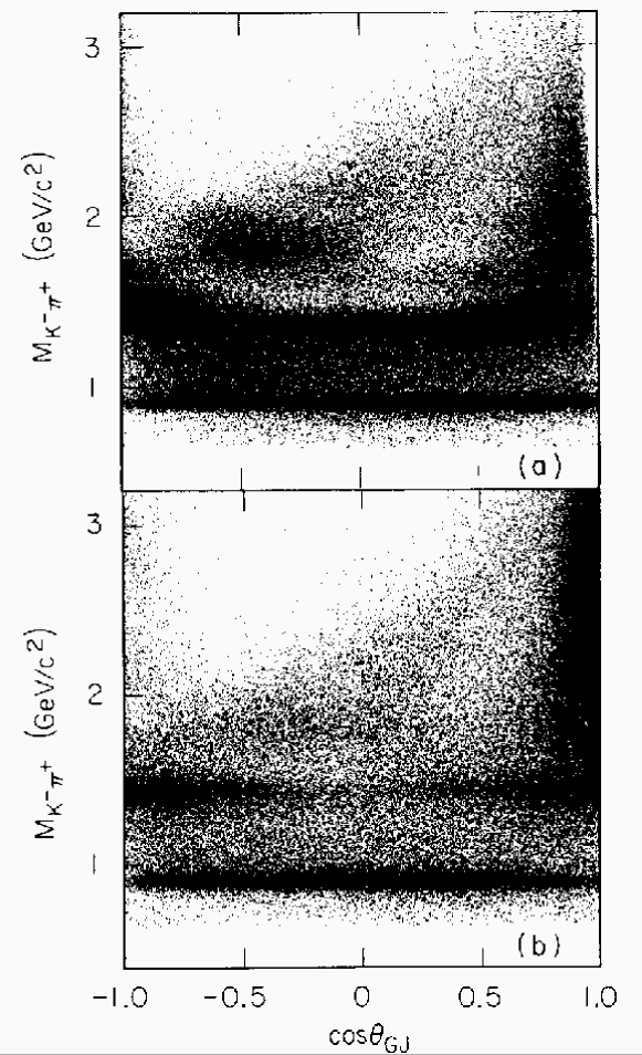
Figure 5.1: The cosine of the Gottfried-Jackson angle of $K^{-}p\to K^{-}\pi^{+}n$ versus the pair mass of $K^{-}\pi^{+}$. Top panel: $|t|\leq 0.2\,\text{GeV}^{2}$. Bottom panel: $0.2\leq|t|\leq 1.0\,\text{GeV}^{2}$; from [17].

The $K^{+}\pi^{+}$ scattering is purely isospin $I=3/2$. The $K^{-}\pi^{+}$ amplitude, studied in [17], also contains an $I=3/2$ component. It is not clear to me whether the forward peak comes only from the isospin components with $I\neq 3/2$. As a hypothesis I nevertheless assume the amplitude $T^{s}(\pi^{+}K^{+}\to\pi^{+}K^{+})$ at energies of about 4–5 GeV, which are of interest here, to share the feature of being forward peaked (or backwards, see footnote 3). From these rough arguments I dare conclude that as a hypothesis we may write for the $\pi^{+}K^{+}$ production amplitude a non-resonant amplitude with an enhancement of its absolute value in the region where $|z_{\pi^{+}K^{+}}|\approx 1$. This is near the boundary of the Dalitz plot. In particular for pair masses of about 4–5 GeV for $\pi^{+}K^{+}$ the enhancement would be near the lower left corner of the Dalitz plot. I denote the amplitude by

$$T(B^{+}\to\pi^{-}(\pi^{+}K^{+}))=\mathcal{A}_{\pi^{+}K^{+}}^{\text{boundary}}.$$ (5.26)

5.2.4 Pronounced S-wave?

Compared to the $K$ and the $D$ the $B$ has a much higher mass ($m_{K}\approx 495\text{MeV}$, $m_{D}\approx 1900\text{MeV}$, $m_{B}\approx 5300\text{MeV}$). The phase space of the three-body final state is therefore much larger in three-body decays of the latter. The region of interest (see equations (5.17)ff.) for present problems of hadron spectroscopy is given by relatively low masses of the $\pi^{-}\pi^{+}$ and $\pi^{-}K^{+}$ pair. By equation (4.18) the pair mass of $\pi^{+}K^{+}$ is therefore about 5 GeV. If the $\pi^{+}K^{+}$ amplitude is indeed forward (or backward) peaked as suggested in section 5.2.3, this could lead to an enhancement near the boundary of the Dalitz plot in the lower left corner. I would be interested in seeing whether such an enhancement explains at least in part the purported observation of an important S wave signal. The risk of mistaking the $\pi^{+}K^{+}$ forward peak for a strong scalar signal of e. g. $f_{0}(980)$ is given because the bands or dips expected for such a state is very close to the left boundary, see figure 5.2.

Figure 5.2: Line with $s_{\pi^{-}\pi^{+}}=(0.980\ \text{GeV})^{2}$ and the boundary of the Dalitz plot for $B^{+}\to\pi^{-}\pi^{+}K^{+}$.

5.2.5 Resulting ansatz

Putting together equations (5.1), (5.20) and (5.26) we obtain for the three-body decay amplitude

$$T(B^{+}\to\pi^{-}\pi^{+}K^{+})=\alpha_{\pi^{-}\pi^{+}}T^{s}(\pi^{-}\pi^{+}\to\pi^{-}\pi^{+})\\ +\alpha_{\pi^{-}K^{+}}T^{s}(\pi^{-}K^{+}\to\pi^{-}K^{+})+\mathcal{A}_{\pi^{+}K^{+}}^{\text{boundary}}.$$ (5.27)

Performing isospin decomposition (with conventions of the Particle Data Group) we get

$$\begin{split}T(B^{+}\to\pi^{-}\pi^{+}K^{+})&=\alpha_{\pi^{-}\pi^{+}}[1/6T_{2}(\pi\pi)+1/2T_{1}(\pi\pi)+1/3T_{0}(\pi\pi)]\\ &\quad+\alpha_{\pi^{-}K^{+}}[1/3T_{3/2}(\pi^{-}K^{+})+2/3T_{1/2}(\pi^{-}K^{+})]\\ &\quad+\mathcal{A}_{3/2}^{\text{boundary}}(\pi^{+}K^{+}).\end{split}$$ (5.28)

Partial-wave decomposition for the $\pi^{-}\pi^{+}$ and the $\pi^{-}K^{+}$ amplitudes (taking into account only S and P wave, i. e. $J=0$ and $J=1$) further yields

$$\begin{split}T(B^{+}\to\pi^{-}\pi^{+}K^{+})&=\frac{1}{4\pi}\big{(}\alpha_{\pi^{-}\pi^{+}}[1/6T^{0}_{2}(\pi\pi)+1/2\cos\theta_{\pi^{-}\pi^{+}}T^{1}_{1}(\pi\pi)+1/3T^{0}_{0}(\pi\pi)]\\ &\quad+\alpha_{\pi^{-}K^{+}}[1/3\{T^{0}_{3/2}(\pi^{-}K^{+})+\cos\theta_{\pi^{-}K^{+}}T^{1}_{3/2}(\pi^{-}K^{+})\}\\ &\quad+2/3\{T^{0}_{1/2}(\pi^{-}K^{+})+\cos\theta_{\pi^{-}K^{+}}T^{1}_{1/2}(\pi^{-}K^{+})\}]\big{)}\\ &\quad+\mathcal{A}_{3/2}^{\text{boundary}}(\pi^{+}K^{+}).\end{split}$$ (5.29)

Because the (real) coupling constants $\alpha$ may be singular (see section 5.2.2) it is appropriate to define the following (still real) coupling constants:

$$\begin{split}(\alpha_{\pi^{-}\pi^{+}})^{J}_{I}&\equiv 2\alpha_{\pi^{-}\pi^{+}}\sin\delta^{J}_{I}(\pi^{-}\pi^{+}),\\ (\alpha_{\pi^{-}K^{+}})^{J}_{I}&\equiv 2\alpha_{\pi^{-}K^{+}}\sin\delta^{J}_{I}(\pi^{-}K^{+}).\end{split}$$ (5.30)

Then equation (5.29) reads

$$\begin{split}T(B^{+}\to\pi^{-}\pi^{+}K^{+})&=\frac{1}{4\pi}\big{(}1/6(\alpha_{\pi^{-}\pi^{+}})^{0}_{2}e^{i\delta^{0}_{2}(\pi\pi)}+1/2\cos\theta_{\pi^{-}\pi^{+}}(\alpha_{\pi^{-}\pi^{+}})^{1}_{1}e^{i\delta^{1}_{1}(\pi\pi)}\\ &\quad+1/3(\alpha_{\pi^{-}\pi^{+}})^{0}_{0}e^{i\delta^{0}_{0}(\pi\pi)}\\ &\quad+1/3\{(\alpha_{\pi^{-}K^{+}})^{0}_{3/2}e^{i\delta^{0}_{3/2}(\pi^{-}K^{+})}+\cos\theta_{\pi^{-}K^{+}}(\alpha_{\pi^{-}K^{+}})^{1}_{3/2}e^{i\delta^{1}_{3/2}(\pi^{-}K^{+})}\}\\ &\quad+2/3\{(\alpha_{\pi^{-}K^{+}})^{0}_{1/2}e^{i\delta^{0}_{1/2}(\pi^{-}K^{+})}+\cos\theta_{\pi^{-}K^{+}}(\alpha_{\pi^{-}K^{+}})^{1}_{1/2}e^{i\delta^{1}_{1/2}(\pi^{-}K^{+})}\}\big{)}\\ &\quad+\mathcal{A}_{3/2}^{\text{boundary}}(\pi^{+}K^{+}).\end{split}$$ (5.31)

In this ansatz the phases of the $\pi^{-}\pi^{+}$ and $\pi^{-}K^{+}$ amplitudes are not free fit parameters but are the strong phases of the respective scattering amplitude. The phase $\delta^{0}_{0}(\pi\pi)$ for example is shown in figure 3.5 (top panel). In the Dalitz plot event distribution, which is essentially given by $|T|^{2}$ the phases show up in interference terms of type

$$\cos(\delta^{0}_{2}(\pi\pi)-\delta^{0}_{0}(\pi\pi)).$$ (5.32)

5.3 Two examples

In the following two subsections I briefly report two analyses of $B^{+}\to K^{+}\pi^{+}\pi^{-}$ and $B^{+}\to K^{+}K^{+}K^{-}$. The idea is to give an impression of how different approaches lead to different conclusions.

5.3.1 Minkowski and Ochs

In ref. [8, table VII] the branching fraction for the decay $B^{+}\to K^{+}\pi^{+}\pi^{-}$ via the resonance $f_{0}(980)$ is found to be $7.55\times 10^{-6}$ while in [9, Table 6] it is concluded to be $19.3\times 10^{-6}$. One of the reasons for such discrepancies in the analysis of the three body decays $B^{+}\to K^{+}\pi^{+}\pi^{-}$ and $B^{+}\to K^{+}K^{+}K^{-}$ is the role played by the object called “non-resonant background” or “gb” respectively. In [9], the gb interferes in the $\pi^{+}\pi^{-}$ channel destructively with both $f_{0}(980)$ and $f_{0}(1500)$ such that the peaks in the corresponding mass projection of the Dalitz plot appears smaller than might be expected or even as a dip, see [9] for details, in particular figure 4. In the channel $K^{+}K^{-}$, on the other hand, the gb interferes constructively with the $f_{0}(1500)$ such that, contrary to the expectations, the number of events in the region of the $f_{0}(1500)$ in the $K^{+}K^{-}$ mass projection is actually much higher than in the $\pi^{+}\pi^{-}$ projection, see [9], in particular figure 5.

Large background phase, no $\boldsymbol{f_{0}(1370)}$

Minkowski and Ochs fit only the mass projections on $\pi^{+}\pi^{-}$ and $K^{+}K^{-}$. According to them a fit that takes into account the two-dimensional Dalitz plot distribution would be preferable but as a first exploration a fit of the one-dimensional mass projection should give a rough picture of the dominant aspects. The ansatz for the rate per pair mass interval is roughly the following ($m=\sqrt{s}$), see [9, eq. 12]

$$\frac{d\Gamma}{dm_{hh}}\propto||T_{gb}|e^{i\delta_{bg}}+c_{2}T_{f_{0}(980)}e^{2i\delta_{bg}}+c_{3}T_{f_{0}(1500)}e^{2i\delta_{bg}}|^{2},\\ hh=\pi^{+}\pi^{-},K^{+}K^{-}.$$ (5.33)

This is a superposition of an amplitude representing the broad resonant glueball, $|T_{gb}|e^{i\delta_{bg}}$, and two amplitudes representing the resonances $f_{0}(980)$ and $f_{0}(1500)$. The two resonances are represented by Breit-Wigner terms with an energy dependent width which, moreover, is characterized by a particular shape function $G$,

$$T_{a}=\frac{m_{a}\Gamma_{a}}{m_{a}^{2}-m^{2}-im_{a}\Gamma_{a}(1+G_{a}(m))},\quad a=gb,f_{0}(980),f_{0}(1500).$$ (5.34)

The relative phases between the three resonant contribution are not free fit parameters but share the common factor of $e^{i\delta_{bg}}$. This has as a consequence that the $f_{0}(980)$ and $f_{0}(1500)$ are not typical Breit-Wigner resonances the phases of which move rapidly through $\pi/2$ but are rotated in the Argand diagram by two times the phase of the glueball amplitude at resonance ($\pi/2$). This ansatz is motivated by the interpretation of the isospin S wave as the red dragon, the broad $0^{++}$ glueball interfering destructively with the narrower resonances $f_{0}(980)$ and $f_{0}(1500)$, see figures 3.5–3.7.

Interestingly enough, the superposition of all three amplitudes leads to an enhancement in the region of $m=\sqrt{s_{hh}}=1300\text{MeV}$, which the Belle Collaboration (see section 5.3.2) would rather interpret as a signal from the controversial $f_{0}(1370)$.

5.3.2 Belle Collaboration

I do not discuss here the event reconstruction, background suppression, and corrections for efficiency and resolution of ref. [8]. I only report briefly the ansatz for fitting of the signal. The model that is used to determine the branching fraction in question consists of the following ansatz for the S-matrix element:

$$\begin{split}S_{A_{J}}(K^{+}\pi^{+}\pi^{-})&=a_{K^{*}}e^{i\delta_{K^{*}}}\mathcal{A}_{1}(\pi^{+}K^{+}\pi^{-}|K^{*}(892)^{0})\\ &\quad+a_{K^{*}_{0}}e^{i\delta_{K^{*}_{0}}}\mathcal{A}_{0}(\pi^{+}K^{+}\pi^{-}|K^{*}_{0}(1430))\\ &\quad+a_{\rho}e^{i\delta_{\rho}}\mathcal{A}_{1}(K^{+}\pi^{+}\pi^{-}|\rho(770)^{0})\\ &\quad+a_{f_{0}}e^{i\delta_{f_{0}}}\mathcal{A}_{0}(K^{+}\pi^{+}\pi^{-}|f_{0}(980))\\ &\quad+a_{f_{X}}e^{i\delta_{f_{X}}}\mathcal{A}_{J}(K^{+}\pi^{+}\pi^{-}|f_{X})\\ &\quad+a_{\chi_{c0}}e^{i\delta_{\chi_{c0}}}\mathcal{A}_{0}(K^{+}\pi^{+}\pi^{-}|\chi_{c0})\\ &\quad+\mathcal{A}_{\text{nr}}(K^{+}\pi^{+}\pi^{-}),\end{split}$$ (5.35)

with [8, eq. (9)]

$$\mathcal{A}_{\text{nr}}(K^{+}\pi^{+}\pi^{-})=a_{1}^{\text{nr}}e^{-\alpha s_{13}}e^{i\delta_{1}^{\text{nr}}}+a_{2}^{\text{nr}}e^{-\alpha s_{23}}e^{i\delta_{2}^{\text{nr}}}.$$ (5.36)

Here I adopt the notation of ref. [8]. In this notation the order of the symbols ‘$K^{+}$’, ‘$\pi^{+}$’ and ‘$\pi^{-}$’ in the brackets of $\mathcal{A}$ indicates that the first two terms in equation (5.35) denote an amplitude in the $K^{+}\pi^{-}$ channel whereas the second to sixth term denote each an amplitude in the $\pi^{+}\pi^{-}$ channel. As to the non-resonant amplitude $\mathcal{A_{\text{nr}}}$, the subscripts ‘13’ and ‘23’ show that this amplitude is the (coherent) sum of one amplitude in the $K^{+}\pi^{-}$ channel and one amplitude in the $\pi^{+}\pi^{-}$ channel.

In order to estimate model dependent uncertainties a fit was also carried out using a non-resonant amplitude with a contribution

$$a_{3}^{\text{nr}}e^{-\alpha s_{12}}e^{i\delta_{3}^{\text{nr}}}$$ (5.37)

from the $K^{+}\pi^{+}$ channel. In the default model, called $K\pi\pi-\text{C}_{0}$, to determine the branching fractions, however such a contribution is not present.

Let me spell out more explicitly what the $\mathcal{A}$’s are. I take as an example $\mathcal{A}_{1}(\pi^{+}K^{+}\pi^{-}|K^{*}(892)^{0})$.

$$\begin{split}\mathcal{A}_{1}(\pi^{+}K^{+}\pi^{-}|K^{*}(892)^{0})&\propto\frac{1}{M^{2}_{R}-s_{13}-iM_{R}\Gamma_{R}^{1}(s_{13})}\\ &\quad\times\left(s_{12}-s_{23}+\frac{(M_{R}^{2}-m_{2}^{2})(m_{3}^{2}-m_{1}^{2})}{s_{13}}\right),\end{split}$$ (5.38)

with

$$\Gamma_{R}^{1}(s_{13})\propto\Gamma_{R}\left(\frac{p_{s13}}{p_{0}}\right)^{2}\left(\frac{M_{R}}{\sqrt{s_{13}}}\right)\frac{1+R^{2}p_{0}^{2}}{1+R^{2}p_{s13}^{2}}.$$ (5.39)

The first factor on the right-hand side of equation (5.38) is a relativistic Breit-Wigner function with energy-dependent width $\Gamma_{R}^{1}(s_{13})$, the second factor describes the angular distribution of the three decay products for a resonance with total spin $J=1$.

For a $J=0$ resonance, like for example the $f_{0}(980)$, the amplitude $\mathcal{A}$ takes a simpler form. The factor for the angular distribution is 1. For $M_{R},\sqrt{s_{23}}\gg m_{\pi}$ the energy dependence of the width can be neglected, $\Gamma_{R}^{0}(s_{23})\approx\Gamma_{R}$. The corresponding density of events in the Dalitz plot is proportional to $\mathcal{A}^{2}$, which gives in case of no interference a band of width $\Gamma_{R}^{2}$ parallel to $s_{13}$ the and perpendicular to the $s_{23}$ axis.

Non-resonant background and $\boldsymbol{f_{X}(1300)}$

In contrast to the ansatz of Minkowski and Ochs the analysis by the Belle collaboration lacks a clear interpretation for the introduction and parametrization of their non-resonant amplitude $\mathcal{A}_{\text{nr}}$. As to the controversial $f_{0}(1370)$, the Belle collaboration finds in their default model $K\pi\pi-\text{C}_{0}$ that the “the mass and width of the $f_{X}(1300)$ state obtained from the fit with the model $K\pi\pi-\text{C}_{0}$ are consistent with those for the $f_{0}(1370)$” [8, p. 15].

5.4 Conclusions

In conclusion, I propose the following guidelines to begin with a Dalitz plot analysis of the decay $B^{+}\to\pi^{-}\pi^{+}K^{+}$ or comparable. It goes without saying that I do not mean to have derived strict rules that are necessary and sufficient for a successful analysis. I only try to stress some points that might be neglected in common fit procedures and want to suggest some steps that seem appropriate in the light of the issues discussed in precedent sections and chapters.

5.4.1 Assumptions to be checked

The guidelines I propose rest in particular on the following assumptions, which remain to be checked.

• The two-body angles defined in section 4.2, the Gottfried-Jackson angle and the angle $\theta$ in two-body cms scattering are directly related.

• For the $\pi^{-}\pi^{+}$ and $\pi^{-}K^{+}$ channel one can use as a constraint elastic unitarity. Inelastic channels can be neglected.

• The $\pi^{+}K^{+}$ amplitude has a forward (or backward or both) peak.

• The coupling of of the $B$ to the $\pi^{+}K^{+}$ does not vanish, see page 5.2.3.

5.4.2 Guidelines

Forming triplets of signal events.

One must not only held fix the signal to background ratio but form triplets of signal events for the entire analysis including in particular different mass projections, as discussed in section 2.1.2.

Two-dimensional binning.

Dalitz plot analysis of a decay like $B^{+}\to\pi^{-}\pi^{+}K^{+}$ differ from older Dalitz plot analysis in that they have not the principal aim to determine spin and parity of the decaying particle from characteristic patterns in the plot, see figures 1.1 and 1.2. Rather the aim is to fit the “landscape” over the plot. To this end two dimensional binning of the data and representation as a lego plot is more appropriate than a distribution of points.

Do not fit whole Dalitz plot.

The interior of the Dalitz plot boundary is approximately 3 times larger than the actual region of interest in the lower left corner with $s_{\pi^{-}\pi^{+}}$ and $s_{\pi^{-}K^{+}}$ between zero and 1.6 GeV, roughly. A fit of the hadronic structures under consideration should only be done in this region of interest. If one fits the whole Dalitz-plot, a certain set of parameters may score better in a $\chi^{2}$ test, but not because it represents better the structures in question but the huge rest of the plot, which is irrelevant for the present problems of hadron spectroscopy.

Elastic phases consistent with scattering data.

Because of the at least approximate validity of elastic unitarity constraints (Watson’s theorem, see section 5.2.2) the phases of the amplitudes $T(B^{+}\to(\pi^{-}\pi^{+})K^{+})$ and $T(B^{+}\to(\pi^{-}K^{+})\pi^{+})$ should be (approximately) equal to the phase shifts established in $\pi\pi$ and $K\pi$ scattering analyses.

Forward (or backward) peak from $\boldsymbol{K^{+}\pi^{+}}$?

Without good reasons the amplitude $T(B^{+}\to\pi^{-}(\pi^{+}K^{+}))$ should not be set to zero. Quite the contrary may be true: This amplitude may be non-vanishing and generate an appreciable enhancement at the lower left boundary of the Dalitz plot. If such a signal is indeed present, care should be taken to separate it from searched for S wave signals; see section 5.2.4.

$\boldsymbol{K^{*}(892)^{0}}$ and $\boldsymbol{z_{\pi^{-}K^{+}}=0}$.

The uncontroversial $K^{*}(892)^{0}$ resonance can serve as reference for fixing overall coupling strength and phases. As a spin 1 particle the contribution from this resonance should vanish with $z_{\pi^{-}K^{+}}$.

Peak from $\boldsymbol{K^{+}\pi^{+}}$ and zero from $\boldsymbol{K^{*}(892)^{0}}$.

I could not establish in detail where the line with $z_{\pi^{-}K^{+}}$ passes through the lower left corner of the Dalitz plot, see figure 4.7. Since the signal from $K^{*}(892)^{0}$ should vanish there the non-vanishing of the $K^{+}\pi^{+}$ amplitude could most be noted.

Charge and flavor conjugated reactions.

Analyses of charge and flavor conjugated reactions to $B^{+}\to\pi^{-}\pi^{+}K^{+}$ like

$$B^{+},\ B^{-},\ B^{0},\ \bar{B^{0}}\to\pi\pi K,\ \eta\eta K,\ \eta\pi K$$ (5.40)

may give additional input to decide between alternative fits, and contributions from different isospin components.

Bibliography

• [1] R. H. Dalitz, “On the Analysis of $\tau$-Meson Data and the Nature of the $\tau$-Meson,” Phil. Mag. 44 (1953) 1068.
• [2] E. Fabri, “A Study of $\tau$-Meson Decay,” Nuovo Cimento 11 (1954), no. 5, 479.
• [3] S. Weinberg, The Quantum Theory of Fields, vol. I. Cambridge University Press, 1995.
• [4] C. Zemach, “Three-Pion Decays of Unstable Particles,” Physical Review 133 (1964), no. 5B, B1201–B1220.
• [5] C. Alff and others Phys. Rev. Letters 9 (1962) 325.
• [6] S. Gasiorowicz, Elementary Particle Physics. John Wiley & Sons, Inc., 1966.
• [7] CLEO Collaboration, “Dalitz analysis of the decay $D^{0}\to K^{-}\pi^{+}\pi^{0}$,” Physical Review D 63 (2001) 092001.
• [8] BELLE Collaboration, K. Abe et al., “Dalitz analysis of the three-body charmless decays $B^{+}\to K^{+}\pi^{+}\pi^{-}$ and $B^{+}\to K^{+}K^{+}K^{-}$.” Belle-Conf-0410 at http://belle.kek.jp/conferences/ICHEP2004/. 2004.
• [9] P. Minkowski and W. Ochs, “B decays into light scalar particles and glueball,” Eur. Phys. J. C39 (2005) 71–86, hep-ph/0404194.
• [10] FOCUS Collaboration, “Dalitz plot analysis of $D_{s}^{+}$ and $D^{+}$ decay to $\pi^{+}\pi^{-}\pi^{+}$ using the $K$-matrix formalism,” Physics Letters B 585 (2004) 200–212.
• [11] D. Morgan and M. R. Pennington, “New data on the $K\bar{K}$ threshold region and the nature of the $f_{0}(S^{*})$,” Physical Review D 48 (1993), no. 3, 1185–1204.
• [12] P. Minkowski and W. Ochs, “Identification of the glueballs and the scalar meson nonet of lowest mass,” The European Physical Journal C 9 (1999) 283–312.
• [13] G. F. Chew and F. E. Low, “Unstable Particles as Targets in Scattering Experiments,” Physical Review 113 (1959), no. 6, 1640–1648.
• [14] S. Eidelman et al., “Review of Particle Physics,” Physics Letters B 592 (2004) 1+.
• [15] K. M. Watson, “The Effect of Final State Interactions on Reaction Cross Sections,” Physical Review 88 (1952), no. 5, 1163–1171.
• [16] BELLE Collaboration, K. Abe et al., “Study of the three-body charmless $B^{+}\rightarrow K^{+}\pi^{+}\pi^{-}$ and $B^{+}\rightarrow K^{+}K^{+}K^{-}$ decays,” 2003. BELLE-CONF-0338, EPS Conference contribution EPS-ID 577.
• [17] LASS Collaboration, D. Aston et al., “A study of $K^{-}\pi^{+}$ scattering in the reaction $K^{-}p\to K^{-}\pi^{+}n$ at 11 $\text{GeV}/c$,” Nuclear Physics B 296 (1988), no. 3, 493–526.
• [18] MARK III Collaboration, Baltrusaitis et al., “Radiative decays of the $J/\psi$ into $\gamma\pi^{+}\pi^{-}$ and $\gamma K^{+}K^{-}$,” Phys. Rev. D 35 (1987) 2077–2091.
• [19] M. H. Alston et al., “Resonance in the $\Lambda\pi$ system,” Physical Review Letters 5 (1960), no. 11, 520.
• [20] G. Höhler, “Note on $N$ and $\Delta$ Resonances. Section II: Against Breit-Wigner parameters—a pole-emic,” The European Physical Journal C3 1 (1998).
• [21] Crystal Barrel Collaboration, A. Abele et al., “The $\rho$-mass, width and line-shape in $\bar{p}p$ annihilation at rest,” Physics Letters B 469 (1999) 270.
• [22] E. Klempt, “Glueballs, hybrids, pentaquarks: Introduction to hadron spectroscopy and review of selected topics,” hep-ph/0404270.
• [23] C. Amsler, “Proton antiproton annihilation and meson spectroscopy with the Crystal Barrel,” Rev. Mod. Phys. 70 (1998) 1293–1340, hep-ex/9708025.
• [24] A. Garmash et al., “Study of three-body charmless $B$ decays,” Physical Review D 65 (2002) 092005.
• [25] C. Baltay et al., “Investigation of $Y^{*}$ and $\bar{Y}^{*}$ production in reactions of the type $p+\bar{p}\to Y+\bar{Y}+\pi$,” Physical Review Letters 11 (1963), no. 7, 346–349.
• [26] BABAR Collaboration, “Amplitude analysis of $B^{\pm}\to\pi^{\pm}\pi^{\mp}\pi^{\pm}$ and $B\to K^{\pm}\pi^{\mp}\pi^{\pm}$,” (2004) hep-ex/0408032.
• [27] A. D. Martin and T. D. Spearman, Elementary Particle Theory. North-Holland Publishing Company, Amsterdam, 1970.
• [28] J. R. Taylor, Scattering Theory: The Quantum Theory on Nonrelativistic Collisions. John Wiley & Sons, Inc., 1972.
• [29] B. Hyams et al., “$\pi\pi$ phase-shift analysis from 600 to 1900 MeV,” Nuclear Physics B 64 (1973) 134–162.
• [30] K. L. Au, D. Morgan, and M. R. Pennington, “Meson dynamics beyond the quark model: Study of final-state interactions,” Physical Review D 35 (1987), no. 35, 1633–1664.
• [31] D. H. Perkins, Introduction to High Energy Physics. Addison-Wesley Publishing Company, Inc., third ed., 1987.
• [32] M. E. Peskin and D. V. Schroeder, An Introduction to Quantum Field Theory. Westview Press, 1995.
• [33] M. R. Pennington, “The production model of Ishida et al. and unitarity,” hep-ph/9710456.
• [34] P. Buettiker, S. Descotes-Genon, and B. Moussallam, “A re-analysis of pi K scattering a la Roy and Steiner,” Eur. Phys. J. C33 (2004) 409–432, hep-ph/0310283.