New contributions to
heavy-quarkonium production

Abstract

We reconsider quarkonium production in a field-theoretical setting and we show that the lowest-order mechanism for heavy-quarkonium production receives in general contributions from two different cuts. The first one corresponds to the usual colour-singlet mechanism. The second one has not been considered so far. We treat it in a gauge-invariant manner, and introduce new 4-point vertices, suggestive of the colour-octet mechanism. These new objects enable us to go beyond the static approximation. We show that the contribution of the new cut can be as large as the usual colour-singlet mechanism at high $P_{T}$ for $J/\psi$. In the $\psi^{\prime}$ case, theoretical uncertainties are shown to be large and agreement with data is possible.

Keywords: heavy-quarkonium production, vector-meson production, gauge invariance, relativistic effects, non-static extension
PACS: 14.40.Gx, 13.85.Ni, 11.10.St, 13.20.Gd

1 Introduction

Years after the first disagreement between data [1, 2] and the colour-singlet model (CSM) [3, 4], the problem of heavy-quarkonium production –in particular at the Tevatron– is still with us. Indeed, it is widely accepted now that fragmentation processes, through the colour-octet mechanism (COM) [5] dominate the production of heavy quarkonia in high-energy hadronic collisions, even for $P_{T}$ as low as 6 GeV. In the COM, one then parametrises the non-perturbative transition from octet to singlet by unknown matrix elements, which are determined to reproduce the data. However, fragmentation processes are known to produce mostly transversely-polarised vector mesons at large transverse momentum [6] and, in the $J/\psi$ and $\psi^{\prime}$ cases, this seems in contradiction with the measurements from CDF [7]. For a comprehensive review on the subject, the reader may refer to [8].

We therefore reconsider the basis of quarkonium ($\mathcal{Q}$) production in field theory, and concentrate on $J/\psi$ and $\psi^{\prime}$ production. We shall see that new contributions are present in the lowest-order diagrams, and we shall also explain how one can build a consistent and systematic scheme to go beyond the static approximation. To this end, we shall use 3-point vertices depending on the relative momentum of the constituent quarks and normalised to the leptonic width of the meson. We shall show that, in order to preserve gauge invariance, it is required to introduce vertices more complicated than the 3-point vertex.

Finally, we shall see that our formalism can be easily applied to the production of excited states. In the case of $\psi^{\prime}$, the theoretical uncertainties are unexpectedly large and allow agreement with the data.

2 Bound states in QCD

All the information needed to study processes involving bound states, such as decay and production mechanisms, can be parametrised by vertex functions, which describe the coupling of the bound state to its constituents and contain the information about its size, the amplitude of probability for given quark configurations and the normalisation of its wave function. In the case of heavy quarkonia, the situation simplifies as they can be approximated by their lowest Fock state, made of a heavy quark and an antiquark, combined to obtain the proper quantum numbers. Furthermore, it has been shown [9] that, for light vector mesons, the dominant projection operator is $\gamma^{\mu}$ and we expect this to hold even better for heavy vector mesons as this approximation gets better in the case of $\phi(s\bar{s})$.

The transition $q\bar{q}\rightarrow{\mathcal{Q}}$ can then be described by the following 3-point function:

$$\Gamma^{(3)}_{\mu}(p,P)=\Gamma(p,P)\gamma_{\mu},$$ (1)

with $P\equiv p_{1}-p_{2}$ the total momentum of the bound state, and $p\equiv(p_{1}+p_{2})/2$ the relative momentum of the bound quarks, as drawn in Figure 1. This choice amounts to describing the vector meson as a massive photon with a non-local coupling.

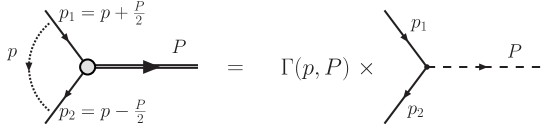
Figure 1: Bound-state vertex obtained by multiplying a point vertex, representing a structureless particle, by a form factor.

We do not assume that the quarks are on-shell : their momentum distribution comes from $\Gamma(p,P)$ and from their propagators. In order to make contact with wave functions, and also to simplify calculations, we assume that $\Gamma(p,P)$ can be taken as a function of the square of the relative c.m. 3-momentum $\vec{p}$ of the quarks, which can be written in a Lorentz invariant form as $\vec{p}^{\,\,2}=-p^{2}+\frac{(p.P)^{2}}{M^{2}}$. For the functional form of $\Gamma(p,P)$, we neglect possible cuts, and choose two otherwise extreme scenarios: a dipolar form which decreases slowly with $\vec{p}$, and a Gaussian form:

$$\Gamma(p,P)=\frac{N}{(1+\frac{\vec{p}^{\,2}}{\Lambda^{2}})^{2}}\text{ and }\Gamma(p,P)=Ne^{-\frac{\vec{p}^{\,2}}{\Lambda^{2}}},$$ (2)

both with a normalisation $N$ and a size parameter $\Lambda$, which can be obtained from relativistic quark models [10]. We shall see in Section 4 how we fix the latter using the leptonic-decay width.

3 Lowest-order production diagrams

In high-energy hadronic collisions, quarkonia are produced at small $x$, where protons are mainly made of gluons. Hence gluon fusion is the main production mechanism. In the case of $J/\psi$ and $\psi^{\prime}$, a final-state gluon emission is required to conserve $C$ parity. This gluon also provides the $\mathcal{Q}$ with transverse momentum $P_{T}$. We assume here that we can use collinear factorisation to describe the initial gluons, and hence that the final-state gluon emission is the unique source of $P_{T}$. All the relevant diagrams for the lowest-order gluon-initiated production process can be obtained from that of Figure 2 by crossing. There are six of them.

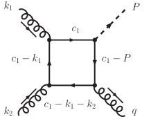
Figure 2: Box diagram.

These diagrams have discontinuities, which generate their imaginary parts. In order to find these, we can use the Landau equations [11]. It is sufficient to consider the diagram of Figure 2, for which the Landau equations become:

$$\lambda_{1}(c_{1}^{2}-m^{2}) = 0$$

$$\lambda_{2}((c_{1}-P)^{2}-m^{2}) = 0$$

$$\lambda_{3}((c_{1}-k_{1})^{2}-m^{2}) = 0$$ (3)

$$\lambda_{4}((c_{1}-k_{1}-k_{2})^{2}-m^{2}) = 0$$

$$\lambda_{1}c_{1}+\lambda_{2}(c_{1}-P)+\lambda_{3}(c_{1}-k_{1})+\lambda_{4}(c_{1}-k_{1}-k_{2}) = 0$$

with $m$ the quark mass. These equations have only two solutions in the physical region: one which is always present and gives a cut which starts at $\hat{s}=(k_{1}+k_{2})^{2}=4m^{2}$, shown in Figure 3 (a), corresponding to a cut through the two $s$-channel propagators, and another one when the meson mass $M$ is larger or equal to $2m$ (see Figure 3 (b): this corresponds to a cut through the two propagators touching the meson). The latter leads to the colour-singlet model [3], which assumes that the quarks should be put on-shell to make the meson. The former cut has not been considered so far for the description of inclusive production. Let us mention however that similar cuts are dominant in diffractive production of vector mesons [12], or in DVCS [13].

We are going to consider this $s$-channel cut in detail. To avoid complications, we choose quark masses $m>M/2$ high enough for the second cut not to contribute. This will also simplify the normalisation procedure for the vertex.

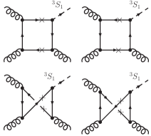
(a) cut 1

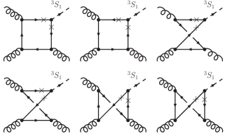
(b) cut 2

Figure 3: The first family (a) has 4 diagrams and the second family (b) 6 diagrams contributing the discontinuity of $gg\to\!\!\ ^{3}S_{1}g$ at LO in QCD.

3.1 Non-locality and gauge invariance

The first problem one immediately faces when evaluating the diagrams ofFigure 3 (a) is that of gauge invariance: whereas these diagrams are gauge invariant if we have a photon instead of a $\mathcal{Q}$, they are not for a finite-size object. Indeed, the vertex function $\Gamma(p,P)$ takes different values in diagrams where either the on-shell quark or the antiquark touches the $\mathcal{Q}$: the relative momentum $p$ is then either $p=2c_{1}-P$ or $p=2c_{2}+P$, so that the delicate cancellation that ensures current conservation is spoilt.

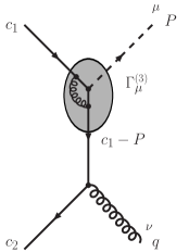
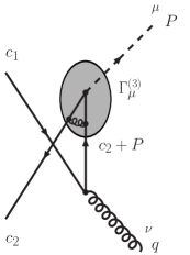
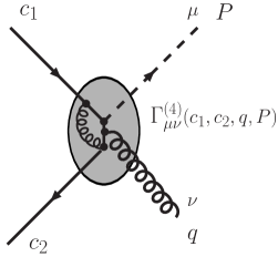
Figure 4: Illustration of the necessity of a 4-point vertex.

The reason is easily understood: if one considers a local vertex, then the gluon can only couple to the quarks that enter the vertex. For a non-local vertex, it is possible for the gluon to connect to the quark or gluon lines inside the vertex, as shown in Figure 4. These contributions must generate a 4-point $q\bar{q}{\mathcal{Q}}g$ vertex, $\Gamma^{(4)}_{\mu\nu}(c_{1},c_{2},q,P)$. In general, its form is unknown, but it must obey some general constraints  [14, 15]:

• it must restore gauge invariance: its addition to the amplitude must lead to current conservation at the gluon vertex;

• it must obey crossing symmetry (or invariance by $C$ conjugation) which can be written

  $$\Gamma^{(4)}_{\mu\nu}(c_{1},c_{2},q,P,m)=-\gamma_{0}\Gamma_{\mu\nu}^{(4)}(-c_{2},-c_{1},q,P,-m)^{\dagger}\gamma_{0};$$ (4)

• it must not introduce new singularities absent from the propagators or from $\Gamma(p,P)$, hence it can only have denominators proportional to $(c_{1}-P)^{2}-m^{2}$ or $(c_{2}+P)^{2}-m^{2}$;

• it must vanish in the case of a local vertex $\Gamma_{\mu}^{(3)}\propto\gamma_{\mu}$, hence we multiply it by $\Gamma(2c_{1}-P,P)-\Gamma(2c_{2}+P,P)$.

These conditions are all fulfilled by the following choice [15]:

$$\Gamma^{(4)}_{\mu\nu}(c_{1},c_{2},P,q) = -ig_{s}T^{a}_{ki}\left[\Gamma(2c_{1}+P,P)-\Gamma(2c_{2}-P,P)\right]$$ (5)

$$\times \left[\frac{c_{1\nu}}{(c_{2}+P)^{2}-m^{2}}+\frac{c_{2\nu}}{(c_{1}-P)^{2}-m^{2}}\right]\gamma_{\mu}$$

where the indices of the colour matrix $T$ are defined in Figure 5, and $g_{s}$ is the strong coupling constant.

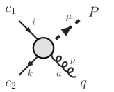
Figure 5: The gauge-invariance restoring vertex, $\Gamma^{(4)}$.

It must be noted first that the quark pair $(c_{1},c_{2})$ that makes the meson is now in a colour-octet state. We thus recover the necessity of such configurations, in this case to restore gauge invariance. We must also point out that this choice of vertex is not unique. We postpone a full study of the 4-point vertex ambiguity [15] to another paper.

When taken into account in the calculation of the discontinuity of $gg\to{\mathcal{Q}}g$, $\Gamma^{(4)}$ introduces two new diagrams shown in Figure 6. Including these contributions in the calculation of the amplitude, we obtain a gauge-invariant quantity.

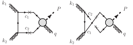
Figure 6: New contributions to the discontinuity of the amplitude from $\Gamma^{(4)}$.

4 Amplitudes

We define ${\mathcal{A}}_{i}^{\mu\nu\rho\sigma}$, $i=1,$…, 6, as the unintegrated amplitude given by the usual Feynman rules for the four diagrams of Figure 3 (a) and the two of Figure 6. We choose the loop momentum $\ell$ so that $c_{1}=\ell+k_{1}$ and $c_{2}=\ell-k_{2}$. We then have for the imaginary part of the physical amplitude ${\mathcal{M}}$:

$${\mathcal{M}}^{pqrs} = \frac{1}{2}\sum_{i=1}^{6}\int\frac{d^{4}\ell}{(2\pi)^{4}}{\mathcal{A}}_{i}^{\mu\nu\rho\sigma}\varepsilon^{p}_{1,\mu}\varepsilon^{q}_{2,\nu}\varepsilon^{r\star}_{3,\rho}\varepsilon^{s\star}_{4,\sigma}$$

$$\times 2\pi\delta^{+}((\ell+k_{1})^{2}-m^{2})2\pi\delta^{-}((\ell-k_{2})^{2}-m^{2})$$

This polarised partonic amplitude is thus obtained by contracting ${\mathcal{A}}_{i}^{\mu\nu\rho\sigma}$ with the polarisation vectors of the gluons $\varepsilon^{p}_{1,\mu}$, $\varepsilon^{q}_{2,\nu}$, $\varepsilon^{s}_{4,\sigma}$ and with that of the vector meson $\varepsilon^{r}_{3,\rho}$, by integrating on the internal phase space restricted by the cutting rules and by summing the six contributions from the diagrams of Figure 3 (a) and Figure 6.

The complete expressions of the polarisation vectors are as follows. One of the transverse polarisations can be taken as orthogonal to the plane of the collision:

$$\varepsilon_{1}^{T_{1}}=\varepsilon_{2}^{T_{1}}=\varepsilon_{3}^{T_{1}}=\varepsilon_{4}^{T_{1}}=\epsilon_{T},$$ (7)

with $\epsilon_{T}.k_{1}=\epsilon_{T}.k_{2}=\epsilon_{T}.P=0$. The other transverse polarisation can be taken as

$$\varepsilon_{1}^{T_{2}}=\sqrt{\frac{1}{\hat{s}\hat{t}\hat{u}}}\left(\hat{t}k_{1}+\hat{u}k_{2}+\hat{s}q\right)=\varepsilon_{2}^{T_{2}}$$ (8)

for the two gluons, and as

$$\varepsilon_{3}^{T_{2}}=\sqrt{\frac{1}{\hat{s}\hat{t}\hat{u}}}\left(\hat{t}k_{1}-\hat{u}k_{2}+\left(\frac{\hat{s}(\hat{t}-\hat{u})}{\hat{t}+\hat{u}}\right)q\right)=\varepsilon_{4}^{T_{2}},$$ (9)

for the final-state gluon and for the vector meson, where $\hat{s}=(k_{1}+k_{2})^{2}$, $\hat{t}=(k_{2}-q)^{2}$ and $\hat{u}=(k_{1}-q)^{2}$ are the Mandelstam variables for the partonic process.

Finally, the longitudinal vector-meson polarisation can be taken as

$$\varepsilon_{3}^{L}=\frac{1}{M}\left(k_{1}+k_{2}-\left(\frac{\hat{s}+M^{2}}{\hat{s}-M^{2}}\right)q\right),$$ (11)

To complete the calculation of the amplitude, we need to normalise the 3-point vertex function $\Gamma^{(3)}$. We use here the leptonic decay width to fix this normalisation [15, 16].

The width in terms of the decay amplitude is given by

$$\Gamma_{\ell\ell}=\frac{1}{2M}\frac{1}{(4\pi^{2})}\int\left|\bar{\mathcal{M}}\right|^{2}d_{2}(PS),$$ (13)

where $d_{2}(PS)$ is the two-particle phase space [17].

The amplitude is obtained as usual through Feynman rules. At lowest order in $\alpha_{s}$, only the 3-point vertex function needs to be considered (giving an explicitly gauge invariant answer). The square of the amplitude is then obtained from the diagram drawn in Figure 7.

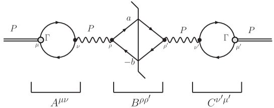
Figure 7: Feynman diagram for ${}^{3}S_{1}\to\ell\bar{\ell}$.

In terms of the sub-amplitudes $A^{\mu\nu}$, $B^{\mu\nu}$ and $C^{\mu\nu}$ defined in Figure 7, we have:

$$\int\left|\bar{\mathcal{M}}\right|^{2}d_{2}(PS)=-\frac{1}{3}\Delta_{\mu\mu^{\prime}}A^{\mu\nu}\frac{g_{\nu\rho}}{M^{2}}B^{\rho\rho^{\prime}}\frac{g_{\rho^{\prime}\nu^{\prime}}}{M^{2}}C^{\nu^{\prime}\mu^{\prime}},$$ (14)

where the factor $\Delta_{\mu\nu}=(g_{\mu\nu}-\frac{P_{\mu}P_{\nu^{\prime}}}{M^{2}})=\sum_{i}\varepsilon_{i,\mu}\varepsilon^{\star}_{i,\mu^{\prime}}$ comes from the sum over polarisations of the meson and the factor $\frac{1}{3}$ from the averaging over the initial polarisations.

$B^{\rho\rho^{\prime}}$, after integration on the two-particle phase space, is found to be

$$B^{\rho\rho^{\prime}}=-e^{2}\frac{2\pi}{3}M^{2}\underbrace{\left[g^{\rho\rho^{\prime}}-\frac{P^{\rho}P^{\rho^{\prime}}}{M^{2}}\right]}_{\Delta^{\rho\rho^{\prime}}}.$$ (15)

$A^{\mu\nu}$ (or equivalently ${C^{\mu\nu}}^{\dagger}$) can be written (see Figure 8):

$$iA^{\mu\nu}=-3e_{Q}\int\!\frac{d^{4}k}{(2\pi)^{4}}\Gamma(k,P)\frac{g^{\mu\nu}(M^{2}+4m^{2}-4k^{2})+8k^{\mu}k^{\nu}-2P^{\mu}P^{\nu}}{((k-\frac{P}{2})^{2}-m^{2}+i\varepsilon)((k+\frac{P}{2})^{2}-m^{2}+i\varepsilon)},$$ (16)

with $e_{Q}$ the heavy-quark charge.

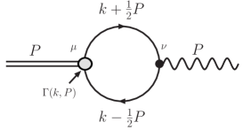
Figure 8: Feynman diagram for ${}^{3}S_{1}\to\gamma^{\star}$.

Performing the $k^{0}$ integration by residues, one obtains

$$A^{\mu\nu}=\frac{-e_{Q}}{\pi^{2}}NI(\Lambda,M,m)\Delta^{\mu\nu}.$$ (17)

with

$$I(\Lambda,M,m)\equiv\int_{0}^{\infty}\!\!\frac{dKK^{2}\Gamma(k,P)}{\sqrt{K^{2}+m^{2}}N}\frac{(2K^{2}+3m^{2})}{(K^{2}+m^{2}-\frac{M^{2}}{4})}.$$ (18)

and $K=|\vec{k}|$. $I$ is a function of $\Lambda$ through the vertex function $\Gamma(k,P)$ and is not in general computable analytically, but it is straightforward to get its numerical value.

Figure 9: Normalisation for a dipole (resp. Gaussian) form of $\Gamma(p,P)$ in the $J/\psi$ case as a function of $\Lambda$: left (resp. right).

We can then put all the pieces together using Eqs. (13) and (14) to determine $N$ from the measured leptonic width. We show in Figure 9 the result in the $J/\psi$ case. As can be seen, the normalisation of the vertex depends rather strongly on $m_{c}$ and $\Lambda$, but very little on the assumed functional dependence of the vertex function. We shall see later that once $N$ is determined from the leptonic rate, the production cross section depends little on these uncertainties.

5 Production cross sections

We can now evaluate the production cross section from the $s$-channel cut. As stated before, we assume that collinear factorisation can be used, in which case the link between the partonic and the hadronic cross sections is given by the following general formula:

$$E\frac{d^{3}\sigma}{dP^{3}}=\int_{0}^{1}dx_{1}dx_{2}\ g(x_{1})\ g(x_{2})\ \frac{\hat{s}}{\pi}\frac{d\sigma}{d\hat{t}}\delta(\hat{s}+\hat{t}+\hat{u}-M^{2}),$$ (19)

where $x_{1}$ and $x_{2}$ are the momentum fractions of the incoming gluons, $P=(E,\vec{P})$ is the momentum of the meson in the c.m. frame of the colliding hadrons, $g(x)$ is the gluon distribution function taken at the scale $\sqrt{M^{2}+P_{T}^{2}}$ .

In the c.m. frame of the colliding hadrons, introducing the rapidity $y=\tanh^{-1}(\frac{P_{z}}{E})$ and the transverse momentum $\vec{P}_{T}$, we obtain the double-differential cross section in $P_{T}$ and $y$ from Eq. (19):

$$\frac{d\sigma}{dydP_{T}}=\int_{0}^{1}dx_{1}dx_{2}g(x_{1})g(x_{2})2\hat{s}P_{T}\frac{d\sigma}{d\hat{t}}\delta(\hat{s}+\hat{t}+\hat{u}-M^{2})$$ . (20)

At this stage, we can perform the integration on $x_{2}$ (or $x_{1}$) using the delta function.

In terms of the transverse energy $E_{T}=\sqrt{P_{T}^{2}+M^{2}}$, we get

$$\hat{s}=sx_{1}x_{2},\ \hat{t}=M^{2}-x_{1}e^{-y}\sqrt{s}E_{T},\ \hat{u}=M^{2}-x_{2}e^{y}\sqrt{s}E_{T},$$ (21)

so that we obtain

$$x_{2}=\frac{x_{1}E_{T}\sqrt{s}e^{-y}-M^{2}}{\sqrt{s}(\sqrt{s}x_{1}-E_{T}e^{y})}.$$ (22)

The double differential cross section on $P_{T}$ and $y$ then takes the following form:

$$\frac{d\sigma}{dydP_{T}}=\int_{x_{1}^{min}}^{1}dx_{1}\frac{2\hat{s}P_{T}g(x_{1})g(x_{2}(x_{1}))}{\sqrt{s}(\sqrt{s}x_{1}-E_{T}e^{y})}\frac{d\sigma}{d\hat{t}},$$ (23)

where $x_{1}^{min}$ corresponds to $x_{2}=1$ in Eq. (22):

$$x_{1}^{min}=\frac{E_{T}\sqrt{s}e^{y}-M^{2}}{\sqrt{s}(E_{T}e^{-y}-\sqrt{s})}.$$ (24)

The last step is to relate the partonic differential cross section $\frac{d\sigma}{d\hat{t}}$ to the amplitude calculated from our model. To this end, we use the well-known formula:

$$\frac{d\sigma^{pqrs}}{d\hat{t}}=\frac{1}{16\pi\hat{s}^{2}}|\overline{\mathcal{M}^{pqrs}}|^{2},$$ (25)

where $|\overline{\mathcal{M}^{pqrs}}|^{2}$ is the squared polarised partonic amplitude for $gg\to{\mathcal{Q}}g$, averaged only over colour for polarised cross sections, and where $p$, $q$, $r$ and $s$ are the helicities of the four particles.

As we are concerned with polarisation only for the $\mathcal{Q}$, we sum over gluon polarisations and define, for $r=L,T_{1},T_{2}$:

$$\frac{d\sigma_{r}}{d\hat{t}}=\sum_{p,q,s=T_{1},T_{2}}\frac{d\sigma^{pqrs}}{d\hat{t}}.$$ (26)

Finally , we have the double-differential polarised cross section on $P_{T}$ and $y$ :

$$\frac{d\sigma_{r}}{dydP_{T}}=\int_{x_{1}^{min}}^{1}dx_{1}\frac{2\hat{s}P_{T}g(x_{1})g(x_{2}(x_{1}))}{\sqrt{s}(\sqrt{s}x_{1}-E_{T}e^{y})}\frac{d\sigma_{r}}{d\hat{t}}.$$ (27)

6 Results for $J/\psi$

Before presenting our results, we need to choose a value for $\Lambda$ and $m_{c}$. Several studies have shown, in the context of relativistic quark models [10], that the scale of the vertex function is between 1.42 and 2.6 GeV, and that $m_{c}$ is between 1.42 and 1.87 GeV. We choose here a value of $\Lambda$ in the middle range, $\Lambda=1.8$ GeV (we shall see that small variations do not affect our results much), and a value of $m_{c}$ equals to the $D^{\pm}$ mass, $m_{c}$=1.87 GeV, in order to have a coherent treatment of all stable charmonium states.

Setting $\sqrt{s}$ to 1800 GeV and considering the cross section in the pseudorapidity range $|\eta|<0.6$, we get the following results for $J/\psi$ production at CDF. The first plot (see Figure 10 (a)) shows our result ($\sigma_{TOT}$, $\sigma_{T}$ and $\sigma_{L}$) for $m=1.87$ GeV and $\Lambda=1.8$ GeV.

These new contributions are compared with the usual LO CSM [3].

It must be stressed that (in the Feynman gauge) the main contribution comes from the 3-point function (Eq. (1)). As can be seen from Figure 10 (b), the term that restores gauge invariance (Eq. (5)) contributes little: the square of its amplitude (see Figure 4 (b)) is about 10 times smaller than the square of the amplitude containing only a 3-point vertex (see Figure 4 (a)). Furthermore, the interference term between the diagrams of Figure 4 (a) and that of Figure 4 (b) is negative, so that the effect of Eq. (5) is to reduce the total amplitude squared. In Figures 11, we show that the normalisation of the results using the decay width has removed most dependence on the choice of parameters. Interestingly, as figure 11 (b) shows, the dependence on $\Lambda$ is negligible once values of the order of 1.4 GeV are taken.

(a) $\sigma_{\rm TOT}$, $\sigma_{T}$ and $\sigma_{L}$

(b) $\sigma_{\rm TOT}$ and $\sigma_{\rm Pert}$,

Figure 10: (a) Polarised ($\sigma_{T}$ and $\sigma_{L}$) and total ($\sigma_{TOT}$) cross sections obtained with a Gaussian vertex function, $m=1.87$ GeV, $\Lambda=1.8$ GeV and the MRST gluon distribution, to be compared with LO CSM. (b) The total (gauge invariant) contribution (plain curve) compared with that of the 3-point vertex of diagrams of Figure 4 (a) (dashed curve) in the Feynman gauge (CTEQ).

We see that the contribution of the new cut matters at large $P_{T}$. Noteworthily, it is much flatter in $P_{T}$ than the LO CSM, and its polarisation is mostly longitudinal. This could have been expected as scalar products of $\varepsilon_{L}$ with momenta in the loop will give an extra $\sqrt{\hat{s}}$ contribution, or equivalently an extra $P_{T}$ power in the amplitude, compared to scalar products involving $\varepsilon_{T}$. One can show that, for $\Lambda=1.8$ GeV, $m_{c}=1.87$ GeV and for MRST structure functions, the longitudinal cross section falls as $1/p_{T}^{8.5}$, whereas the transverse cross section behaves asymptotically as $1/p_{T}^{10.5}$. The asymptotic power of $p_{T}$ changes by 5 % for $\Lambda$ varying between 1.4 and 2.2 GeV.

Recall that in our calculation the LO CSM is zero because $M<2m$. For $M\geq 2m$, we should have added our contribution to that of the LO CSM at the amplitude level. The net result would then be flatter and larger. However, it is clear that the enhancement factor would not be large enough to reach agreement with the data.

(a) Vertex function

(b) $\Lambda$

(c) $\Lambda$ and $m_{c}$

Figure 11: (a) Comparison between the polarised cross sections obtained with the dipole and the Gaussian vertex functions (MRST); (b) Variation of the total cross section due to a change in $\Lambda$ for a fixed value of the quark mass (MRST); (c) Variation of the total cross section due to a change in $m$ and $\Lambda$ (CTEQ).

7 Results for $\psi^{\prime}$

Although the normalisation to the leptonic width removes most of the ambiguities in the $J/\psi$ case, it is not so for radially excited states, such as the $\psi^{\prime}$. Indeed, in this case, the vertex function must have a node. We expect it to appear through a pre-factor, $1-\frac{|\vec{p}|}{a_{node}}$, multiplying the $1S$ vertex function. Explicitly, $\Gamma_{2S}(p,P)$, for a node $a_{node}$ should be well parametrised by

$$\left(1-\frac{|\vec{p}|}{a_{node}}\right)\frac{N^{\prime}}{(1+\frac{|\vec{p}|^{2}}{\Lambda^{2}})^{2}}\text{ or }N^{\prime}\left(1-\frac{|\vec{p}|}{a_{node}}\right)e^{\frac{-|\vec{p}|^{2}}{\Lambda^{2}}}.$$ (28)

In order to determine the node position in momentum space, we can fix $a_{node}$ from its known value in position space, e.g. from potential studies, and take the Fourier transform of the wave function. However, the position of the node is not very well-known, and it is unclear how to relate our vertex with off-shell quarks to an on-shell non-relativistic wave function. The most remarkable thing is that, because the integrand has a zero, the integral $I$ of Eq. (18) entering the decay width calculation can vanish for a certain value $a_{node}=a_{0}$, which turns out to be close to the estimated value of the zero in the wave function. Because of their different momentum dependence, the integrals that control the production are not zero for $a_{node}=a_{0}$. Hence our normalisation procedure can in principle produce an infinite answer. Of course, this means that one cannot be at $a_{node}=a_{0}$ exactly. However, if one is close to it, then it becomes possible to produce a large normalisation. Hence in the $\psi^{\prime}$ case, our procedure can produce agreement with the data at low $P_{T}$.

Figure 12 shows that for $a_{node}=1.334$ GeV, one obtains a good fit to CDF data at moderate $P_{T}$ (note that the slopes are quite similar. This is at odds with what is commonly assumed since fragmentation processes –with a typical $1/P_{T}^{4}$ behaviour– can also describe the data). The $\psi^{\prime}$ is predicted to be mostly longitudinal.

Figure 12: Polarised ($\sigma_{T}$ and $\sigma_{L}$) and total ($\sigma_{TOT}$) cross sections for $\psi^{\prime}$ obtained with a Gaussian vertex functions, $a_{node}=1.334$ GeV, $m=1.87$ GeV, $\Lambda=1.8$ GeV and the CTEQ gluon distribution, to be compared with LO CSM, CSM fragmentation [4] and the data from CDF [1].

This effect of the node in the $\psi^{\prime}$ vertex function could also solve the $\rho-\pi$ puzzle as suggested in [16], since a slight modification in the integrand of $I$ can produce a large suppression in the $\rho-\pi$ decay of the $\psi^{\prime}$. Such a modification in the integrand is indeed expected to come from the presence of an off-shell $\omega$ in the $\rho-\pi$ decay instead of an off-shell photon for the leptonic decay. On the other hand, in the case of $J/\psi$, no important effect are expected.

8 Conclusion and outlook

In this letter, we have shown that there are two singularities in the box diagram contribution to quarkonium production. We have chosen quark masses so that only the $s$-channel singularity (which is usually neglected) contributes, and vertices without cuts.

On the theoretical side, we have begun to map the ingredients needed to go beyond the static approximation $M=2m$. They involve the introduction of new 4-point vertices that restore gauge invariance. We postpone a full study of these to a later publication [20].

On the phenomenological side, we have shown that in the $J/\psi$ case, this new singularity produces results comparable to those of the lowest-order CSM, i. e. too small to accommodate the Tevatron data. In the $\psi^{\prime}$ case, ambiguities in the position of the node of the vertex function can lead to an enhancement, and to an agreement with the data. Hence it is not clear that the same mechanism has to be at work for $1S$ and $2S$ mesons.

Our approach can be used in the case of $P$ waves, where we would simply input a suitable 3-point vertex instead of taking higher derivatives of the wave function and of the perturbative amplitude, but also in a $k_{t}$-factorisation framework [21] (which would enhance the cross section in the $J/\psi$ case), and can be combined with contribution from COM fragmentation. Because the quarkonium are mostly longitudinal in this work and transverse in fragmentation, it seems possible to reach agreement with polarisation data.

References

- [1] F. Abe et al. [CDF Collaboration], Phys. Rev. Lett. 79 (1997) 572.
- [2] F. Abe et al. [CDF Collaboration], Phys. Rev. Lett. 79 (1997) 578.
- [3] C-H. Chang, Nucl. Phys. B 172 (1980) 425; R. Baier and R. Rückl, Phys. Lett. B 102 (1981) 364; R. Baier and R. Rückl, Z. Phys. C 19 (1983) 251.
- [4] M. Cacciari and M. Greco, Phys. Rev. Lett. 73 (1994) 1586 [arXiv:hep-ph/9405241]; E. Braaten, M. A. Doncheski, S. Fleming and M. L. Mangano, Phys. Lett. B 333 (1994) 548 [arXiv:hep-ph/9405407].
- [5] G. T. Bodwin, E. Braaten and G. P. Lepage, Phys. Rev. D 51 (1995) 1125 [Erratum-ibid. D 55 (1997) 5853] [arXiv:hep-ph/9407339]; P. L. Cho and A. K. Leibovich, Phys. Rev. D 53 (1996) 150 [arXiv:hep-ph/9505329]; P. L. Cho and A. K. Leibovich, Phys. Rev. D 53 (1996) 6203 [arXiv:hep-ph/9511315].
- [6] P. L. Cho and M. B. Wise, Phys. Lett. B 346 (1995) 129 [arXiv:hep-ph/9411303].
- [7] T. Affolder et al. [CDF Collaboration], Phys. Rev. Lett. 85 (2000) 2886 [arXiv:hep-ex/0004027].
- [8] N. Brambilla et al., CERN Yellow Report on “Heavy quarkonium physics”, CERN-2005-005 [arXiv:hep-ph/0412158].
- [9] C. J. Burden, L. Qian, C. D. Roberts, P. C. Tandy and M. J. Thomson, Phys. Rev. C 55 (1997) 2649 [arXiv:nucl-th/9605027].
- [10] M. A. Ivanov, J. G. Korner and P. Santorelli, Phys. Rev. D 71 (2005) 094006 [arXiv:hep-ph/0501051], Phys. Rev. D 70 (2004) 014005 [arXiv:hep-ph/0311300], Phys. Rev. D 63 (2001) 074010 [arXiv:hep-ph/0007169]; M. A. Nobes and R. M. Woloshyn, J. Phys. G 26 (2000) 1079 [arXiv:hep-ph/0005056].
- [11] L. D. Landau, Nucl. Phys. 13 (1959) 181; C. Itzykson, J.B. Zuber, Quantum Field Theory, McGraw-Hill, New-York, 1980.
- [12] see e.g. J. R. Cudell and I. Royen, Phys. Lett. B 397 (1997) 317 [arXiv:hep-ph/9609490]; M. G. Ryskin, Z. Phys. C 57 (1993) 89; J. R. Cudell, Nucl. Phys. B 336 (1990) 1.
- [13] A. V. Radyushkin, Phys. Rev. D 56 (1997) 5524 [arXiv:hep-ph/9704207].
- [14] S. D. Drell and T. D. Lee, Phys. Rev. D 5 (1972) 1738.
- [15] J. P. Lansberg, Quarkonium Production at High-Energy Hadron Colliders, Ph.D. Thesis, ULg, Liège, Belgium, 2005 [arXiv:hep-ph/0507175].
- [16] J. P. Lansberg, AIP Conf. Proc. 775 (2005) 11 [arXiv:hep-ph/0507184].
- [17] V.D. Barger and R.J.N. Philips, Collider Physics, Addison-Wesley, Menlo Park, 1987.
- [18] A. D. Martin, R. G. Roberts, W. J. Stirling and R. S. Thorne, Phys. Lett. B 531 (2002) 216 [arXiv:hep-ph/0201127].
- [19] J. Pumplin, D. R. Stump, J. Huston, H. L. Lai, P. Nadolsky and W. K. Tung, JHEP 0207 (2002) 012 [arXiv:hep-ph/0201195].
- [20] J.R. Cudell, Yu.L. Kalinovsky and J.P. Lansberg, in preparation.
- [21] P. Hagler, R. Kirschner, A. Schafer, L. Szymanowski and O. V. Teryaev, Phys. Rev. Lett. 86 (2001) 1446 [arXiv:hep-ph/0004263]; P. Hagler, R. Kirschner, A. Schafer, L. Szymanowski and O. V. Teryaev, Phys. Rev. D 63 (2001) 077501 [arXiv:hep-ph/0008316].