Pion Parton Distributions in a non local Lagrangian.

Abstract

We use phenomenological nonlocal Lagrangians, which lead to non trivial forms for the quark propagator, to describe the pion. We define a procedure based on previous studies on non local lagrangians for the calculation of the pion parton distributions at low $Q^{2}$ . The obtained parton distributions fulfill all the wishful properties. Using a convolution approach we incorporate the composite character of the constituent quarks. We evolve, using the Renormalization Group, the calculated parton distributions to the experimental scale and compare favorably with the data and draw conclusions.

I Introduction

Parton Distributions Functions (PDFs) and Generalized Parton Distributions (GPDs) MullerRobaschikGeyerDittesHorejsiFortsch94-98 ; Radyushkin97 ; Ji97 , relating PDFs and electromagnetic form factors, encode unique information on the non perturbative hadron structure (for a recent review, see Diehl03 ). Any realistic model of hadron structure should be able to calculate them. We shall proceed in here to study the parton distribution functions of the pion in a previous developed formalism Noguera05 .

From the experimental point of view the PDFs and GPDs of the pion are difficult to determine. Pions decay into muons or photons and therefore the pion distribution functions can not be obtained from direct DIS experiments. The pion parton distribution has been inferred from the Drell-Yang process BadierNA3 ; BetevNA10 ; Conway89 and direct photon production Aurencheetall89 in pion-nucleon and pion-nucleus collisions. These set of experiments have been analyzed in ref. SuttonMartinRobertsStirling92 obtaining that the fraction of moment of each valence (anti)quark in the pion is about 0.23 for $Q^{2}=4\operatorname{GeV}^{2}.$

The parton distribution functions of the pion has been a subject of much discussion in the literature. In BestSchafer97 ; DetmoldMelnitchoukThomas03 calculations using quenched lattice QCD, for their lowest moments, were performed. The lack of sea quarks in the approximation implies a greater presence of valence quarks. Its PDFs DavidsonRuizArriola ; RuizArriolaBroniowski02 and GPDs NogueraTheusslVento04 have been also calculated in the Nambu-Jona Lasinio (NJL) model Nambu . In the chiral limit, its quark valence distribution is as simple as $q\left(x\right)=\theta\left(x\right)\theta\left(1-x\right).$ Once evolution is taken into account, good agreement is reached between the calculated PDFs and the experimental resultsDavidsonRuizArriola . The pion PDFs and GPDs have also been calculated in a model with the simplest pseudoscalar coupling between the pion and the constituent quark fields Lansberg , and in the instanton model, PolyakovWeiss99 ; Polyakov99 . In ref. PolyakovWeiss99 the chiral limit result of the NJL model for PDFs changes such that $q\left(x\right)$ goes to zero for $x\rightarrow 0$ and $x\rightarrow 1.$ The pion PDFs have also been calculated in a spectral quark modelRuizArriolaBroniowski03 .

Also, the pion PDFs have been calculated in a statistical model, without any dynamical assumption, obtaining quite reasonable results AlbergHenley05 . In AnikinBinosiMedranoNogueraVento02 the GPDs of the pion are calculated in the bag model. A relevant contribution to the calculation of the pion GPDs on the light-front has been given by Tiburzi and Miller TiburziMiller , and some remarks on the use of the light-front for calculating GPDs can be found in Simula . Looking for a more fundamental approach, not related to a unique model, the pion PDF has been also calculated in the framework of Dyson-Schwinger Equations HechtRobertsSchmidt01 .

In all the previous calculations the pion was built of two valence constituent (anti)quarks. However, these constituent (anti)quarks are themselves built of elementary partons. The way to connect a description in terms of constituent quarks with the description in terms of the elementary partons was described in AltarelliCabibboMaianiPetronzio74 ; NogueraScopettaVento . Hereafter, we will call this procedure ACMP. In AltarelliCabibboMaianiPetronzio74 ; Scopetta1 ; Scopetta2 the procedure was applied to the nucleon case and in AltarelliPetrarcaRapuano96 it was applied to the pion case. The same description of the constituent quarks in terms of partons is used for the proton and for the pion.

The aim of this paper is to study the pion PDFs following the ideas developed in ref Noguera05 ; NogueraTheusslVento04 . Our main objective is to develop a calculational method for the PDFs preserving all the fundamental symmetries, i.e. momentum conservation and gauge symmetry. Another motivation is to understand the simple result obtained for the pion PDFs in the NJL model in connection with our more elaborate description.

Our study is done in a lagrangian model Noguera05 built with the following properties: (i) manifest chiral invariance for the strong part of the interaction; (ii) a momentum dependence for the quark propagator provided by QCD based calculations; (iii) the implementation of local gauge invariance provides the electromagnetic interaction. This procedure allows us to have simultaneously a coherent description of the dressed quark propagator, the pion state, the dressed quark photon vertex and to preserve gauge symmetry. In this sense our aim is not to fit the best possible description of the pion PDFs, but to learn about the influence of the momentum dependence of the quark propagator on the definition of the PDFs. The differences between our approach and the previous calculation HechtRobertsSchmidt01 will become obvious. We achieve our objective in a three step process. The first is to construct the PDFs of the pion in terms of its constituents quarks, for that we will use the model developed in ref. Noguera05 . For this model the pion form factor was calculated obtaining good agreement with data, and the operator form for the mesonic parton distribution was found in terms of the quark propagator and the kernel of the BS equation. The second step is to include the partonic structure of the constituent quarks. To do so we will use the ACMP procedure assuming for the quarks the same structure functions as was obtained in the analysis for the proton. The last step is to evolve (to next to leading order), by means of the renormalization group of QCD, the resulting parton distribution up to the value of $Q^{2}$ for which data exist Traini .

This paper is organized as follows. In section II we discuss the definition of the PDFs in our formalism and give provide some technical details of the calculation. In section III we perform an analysis of the PDFs, with models defined from fundamental approaches, achieving a good description of the data. In section IV we calculate the moments of the parton distribution, using three different procedures, to check the validity of our method for calculating parton distributions, and in section V we provide some conclusions.

II The constituent parton distribution functions

In our scheme the pion arises as a solution of the two body BS and therefore is a composite system of two “constituent” valence (anti)quarks which determine the PDFs. To calculate them the corresponding operator was introduced in ref Noguera05 (we refer the reader to this paper for details).

The parton distribution has three contributions:

$$q_{u}\left(x\right)=q_{u}^{\left(1\right)}\left(x\right)+\tilde{q}_{u}^{\left(1\right)}\left(x\right)+q_{u}^{\left(2\right)}\left(x\right).$$ (1)

The first one, $q_{u}^{\left(1\right)}\left(x\right)$, corresponds to the one body term

$$q_{u}^{\left(1\right)}\left(x\right)=-\int\frac{d^{4}p}{\left(2\pi\right)^{4}}\text{ }\delta\left(x-\frac{n}{2}\cdot\left(2p+P\right)\right)\,\mathbb{T}\mathrm{r}\left[i\,S\left(p-\frac{1}{2}P\right)\bar{\Gamma}^{M}\left(p,P\right)i\,S\left(p+\frac{1}{2}P\right)\right.$$

$$\left.\Gamma_{\mu}\left(p+\frac{1}{2}P,p+\frac{1}{2}P\right)n^{\mu}\,i\,S\left(p+\frac{1}{2}P\right)\Gamma^{M}\left(p,P\right)\right]$$ (2)

where $\mathbb{T}$r represent the trace in Dirac, color and flavor indices, $\Gamma^{\mu}\left(p,p^{\prime}\right)$ is the quark-photon vertex which in general can have a complicated structure (see Noguera05 ; BallChiu80 ; CurtisPennington90 ). Here $\Gamma^{M}\left(p,P\right)$ is the BS amplitude for the meson,

$$\Gamma_{\gamma\alpha}^{M}\left(p,P\right)=-2i\int\frac{d^{4}p^{\prime}}{\left(2\pi\right)^{4}}G_{\alpha\beta\gamma\delta}\left(p,p^{\prime},P\right)\left(i\,S\left(p^{\prime}+\frac{1}{2}P\right)~{}\Gamma^{M}\left(p^{\prime},P\right)\,i\,S\left(p^{\prime}-\frac{1}{2}P\right)\right)_{\beta\delta}$$ (3)

with $\alpha,\beta,\gamma$ and $\delta$ including spinor, color and flavor indices. The normalization condition for the BS amplitude is:

$$2iP^{\mu}=$$

$$\int\frac{d^{4}p}{\left(2\pi\right)^{4}}\mathbb{T}\text{r}\left[\bar{\Gamma}^{M}\left(p,P\right)i\,\frac{\partial S\left(p+\frac{1}{2}P\right)}{\partial P_{\mu}}\,\Gamma^{M}\left(p,P\right)\,i\,S\left(p-\frac{1}{2}P\right)+\bar{\Gamma}^{M}\left(p,P\right)i\,S\left(p+\frac{1}{2}P\right)\,\Gamma^{M}\left(p,P\right)\,i\,\frac{\partial S\left(p-\frac{1}{2}P\right)}{\partial P_{\mu}}\right]-$$

$$2i\int\frac{d^{4}p}{\left(2\pi\right)^{4}}\frac{d^{4}p^{\prime}}{\left(2\pi\right)^{4}}\left[i\,S\left(p-\frac{1}{2}P\right)\bar{\Gamma}^{M}\left(p,P\right)i\,S\left(p+\frac{1}{2}P\right)\right]_{\alpha\gamma}\frac{\partial G_{\alpha\beta\gamma\delta}\left(p,p^{\prime},P\right)}{\partial P_{\mu}}\left[i\,S\left(p^{\prime}+\frac{1}{2}P\right)\,\Gamma^{M}\left(p^{\prime},P\right)\,i\,S\left(p^{\prime}-\frac{1}{2}P\right)\right]_{\beta\delta}.$$ (4)

To calculate the PDF we need the elastic vertex $\Gamma^{\mu}\left(p,p\right)$ directly related to the quark propagator by using the Ward Identity:

$$\Gamma^{\mu}\left(p,p\right)=\frac{\partial S^{-1}\left(p\right)}{\partial p_{\mu}}~{}.$$ (5)

The pion momentum can be expressed in terms of the light-front vectors as $P^{\mu}=\bar{p}^{\mu}+m_{\pi}^{2}n^{\mu}/2$ with $\bar{p}^{\mu}=\bar{P}\left(1,0,0,1\right)/\sqrt{2},$ $n^{\mu}=\left(1,0,0,-1\right)/(\sqrt{2}\bar{P}),$ where $\bar{P}$ has a particular value for each frame (for instance $\bar{P}=M/\sqrt{2}$ for the rest frame). This first contribution corresponds to diagram shown in Fig. 1.

The second term is also a one body term:

$$\tilde{q}_{u}^{\left(1\right)}\left(x\right)=\int\frac{d^{4}p}{\left(2\pi\right)^{4}}\frac{1}{4}\delta\left(x-\frac{n}{2}\cdot\left(2p+P\right)\right)\mathbb{T}\mathrm{r}\left[in_{\mu}~{}\frac{d\bar{\Gamma}^{M}\left(p,P\right)}{dp_{\mu}}\,i\,S\left(p+\frac{1}{2}P\right)\Gamma^{M}\left(p,P\right)i\,S\left(p-\frac{1}{2}P\right)\right.$$

$$+\left.i\,S\left(p-\frac{1}{2}P\right)\bar{\Gamma}^{M}\left(p,P\right)i\,S\left(p+\frac{1}{2}P\right)in_{\mu}~{}\frac{d\Gamma^{M}\left(p,P\right)}{dp_{\mu}}\right]$$ (6)

while the third term is a genuine two body term given by:

$$q_{u}^{\left(2\right)}\left(x\right)=\int\frac{d^{4}p}{\left(2\pi\right)^{4}}\int\frac{d^{4}p^{\prime}}{\left(2\pi\right)^{4}}\,\left[i\,S\left(p^{\prime}-\frac{1}{2}P\right)\bar{\Gamma}^{M}\left(p^{\prime},P\right)i\,S\left(p^{\prime}+\frac{1}{2}P\right)\right]_{\alpha\gamma}$$

$$\frac{1}{2}n_{\mu}~{}\left\{\left[\delta\left(x-\frac{n}{2}\cdot\left(2p+P\right)\right)\left(\frac{d}{dp_{\mu}^{\prime}}+2\frac{d}{dP_{\mu}}\right)+\delta\left(x-\frac{n}{2}\cdot\left(2p^{\prime}+P\right)\right)\left(\frac{d}{dp_{\mu}}+2\frac{d}{dP_{\mu}}\right)\right]G_{\alpha\beta\gamma\delta}\left(p^{\prime},p,P\right)\right\}$$

$$\left[\,i\,S\left(p+\frac{1}{2}P\right)\Gamma^{M}\left(p,P\right)i\,S\left(p-\frac{1}{2}P\right)\right]_{\beta\delta}$$ (7)

These two last contributions corresponds to the diagram of Fig 2 and they result from the non local character of the interactions . In the contribution $\tilde{q}_{u}^{\left(1\right)}\left(x\right)$ the bubble integral has been performed using the BS equation, whereas this is not possible in the contribution $q_{u}^{\left(2\right)}\left(x\right).$

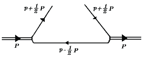
Figure 1: Diagrammatic expression of the first one body term in Eq.(1)

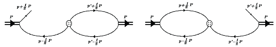
Figure 2: Diagrammatic expression of the second one body term and the two body term in Eq.(1)

In ref. Noguera05 a particular model was developed defined by means of a chirally invariant lagrangian:

$$\mathcal{L}\left(x\right)=\bar{\psi}\left(x\right)\left(i\ \hbox to0.0pt{$/$\hss}\partial-m_{0}\right)\psi\left(x\right)+g_{0}\left[J_{S}^{\dagger}\left(x\right)J_{S}\left(x\right)+\vec{J}_{5}^{\;\dagger}\left(x\right)\vec{J}_{5}\left(x\right)\right]+g_{p}\ J_{p}^{\dagger}\left(x\right)J_{p}\left(x\right)$$ (8)

built with the non local currents defined by

$$J_{S}\left(x\right) =\int d^{4}y\,G_{0}\left(y\right)\bar{\psi}\left(x+\frac{1}{2}y\right)\psi\left(x-\frac{1}{2}y\right)$$

$$\vec{J}_{5}\left(x\right) =\int d^{4}y\,G_{0}\left(y\right)\bar{\psi}\left(x+\frac{1}{2}y\right)i\vec{\tau}\gamma_{5}\psi\left(x-\frac{1}{2}y\right)$$ (9)

$$J_{p}\left(x\right) =\int d^{4}y\,G_{p}\left(y\right)\bar{\psi}\left(x+\frac{1}{2}y\right)\frac{1}{2}i\overleftrightarrow{\hbox to0.0pt{$/$\hss}\partial}\psi\left(x-\frac{1}{2}y\right)$$

where $u\overleftrightarrow{\partial}v=u\left(\partial v\right)-\left(\partial u\right)v.$ The first and second currents require the same $G_{0}\left(y\right)$, in order to implement chiral invariance, while the third current is self-invariant under chiral transformations. The scalar current, $J_{S},$ generates a momentum dependent mass, and the last current, the “momentum” current, $J_{p},$ is responsible for the momentum dependence of the wave function renormalization. The pseudo-scalar current, $\vec{J}_{5},$ generates the pion pole. For simplicity, we assume that all the $G\left(y\right)$ functions are real.

Let us define

$$G\left(p\right)=\int d^{4}y\,e^{iyp}G\left(y\right)$$ (10)

with the normalization condition $G\left(p=0\right)=1.$ For simplicity we consider that our effective theory arises from the large $N_{c}$ limit of $QCD$. This is equivalent to working in the Hartree approximation, i.e. only direct diagrams will be considered.

The model introduces, in a natural way, momentum dependence to the quark mass and to the wave function renormalization of the quark propagator:

$$S\left(p\right)=Z\left(p\right)\frac{\hbox to0.0pt{$/$\hss}p+m\left(p\right)}{p^{2}-m^{2}\left(p\right)+i\epsilon}$$ (11)

where the explicit expressions for $m\left(p\right)$ and $Z\left(p\right)$ are given in the Appendix A. The scalar current can give a mass for the quark even if the Lagrangian contains no explicit mass term, $m_{0}=0,$ leading to a spontaneous symmetry breaking mechanism similar to that in the Nambu-Jona Lasinio model. On the other hand, the momentum current gives rise to a momentum dependent wave function normalization. However, even though the latter contributes to the mass, it is not able by itself to break chiral symmetry spontaneously.

The model defined in Eq. (8) gives the following interaction terms,

$$G_{\alpha\beta\gamma\delta}\left(p^{\prime},p,P\right)=2\ g_{0}\ G_{0}\left(p^{\prime}\right)G_{0}\left(p\right)\left[\delta_{\gamma\alpha}\delta_{\delta\beta}+\left(i\vec{\tau}\gamma_{5}\right)_{\gamma\alpha}\left(i\vec{\tau}\gamma_{5}\right)_{\delta\beta}\right]+2\ g_{p}\ G_{p}\left(p^{\prime}\right)G_{p}\left(p\right)\left(\hbox to0.0pt{$/$\hss}p^{\prime}\right)_{\gamma\alpha}\left(\hbox to0.0pt{$/$\hss}p\right)_{\delta\beta}$$ (12)

and the corresponding BS equation (3) can be easily solved leading to:

$$\Gamma^{M=\pi^{i}}\left(p,P\right)=\,i\,\gamma_{5}\,\tau^{i}\,g_{\pi qq}G_{0}\left(p\right)$$ (13)

In Appendix A we give the explicit expressions fixing the pion mass and the normalization constant $g_{\pi qq}$. This model realizes the Goldstone theorem and therefore $m_{\pi}$ goes to zero when $m_{0}$ vanishes. This is a consequence of the use of the same $G_{0}\left(p\right)$ function in the scalar current, $J_{S},$ and pseudoscalar current, $\vec{J}_{5},$ in Eq. (9). On the other hand, we have no constrain on $G_{p}\left(p\right)$ imposed by chiral symmetry.

Inserting Eqs.(12) and (13) in Eq. (7) we obtain

$$q_{u}^{\left(2\right)}\left(x\right)=0.$$ (14)

Summarizing, our scheme leads to two contributions: the standard one, associated with the triangle diagram, and defined in (2) and a new contribution defined in Eq. (6). This latter contribution arises from the non locality of the currents in our model, it is also a triangle diagram, from the point of view of QCD, but once written in terms of the BS amplitudes it gets a different structure.

We now proceed to the explicit calculation of the PDF. First of all we can use the $\delta$-function present in Eqs. (2) and (6) in order to integrate over $p^{3}:$

$$\delta\left(x-\frac{n}{2}\cdot\left(2p+P\right)\right)=\sqrt{2}\bar{P}~{}\delta\left(\sqrt{2}\bar{P}\left(x-\frac{1}{2}\right)-p^{0}-p^{3}\right)$$ (15)

With this integration, all the quantities appearing in Eqs. (2) and (6) become linear in $p^{0}.$ In order to show explicitly that the results do not depend on the choice of $\bar{P}$ we use the following variable

$$2\sqrt{2}\bar{P}\left(p^{0}-\frac{\bar{P}}{\sqrt{2}}\left(x-\frac{1}{2}\right)\right)=\omega+m_{\pi}^{2}\left(\frac{1}{2}-x\right).$$ (16)

The last term has been introduced in order to obtain symmetric expressions. In terms of $\omega$ we have

$$p^{2} =\omega\left(x-\frac{1}{2}\right)-m_{\pi}^{2}\left(\frac{1}{2}-x\right)^{2}-\vec{p}_{\bot}^{2}~{}~{},$$

$$\left(p-\frac{1}{2}P\right)^{2} =-\omega\left(1-x\right)+m_{\pi}^{2}x\left(1-x\right)-\vec{p}_{\bot}^{2}~{}~{},$$ (17)

$$\left(p+\frac{1}{2}P\right)^{2} =\omega x+m_{\pi}^{2}\left(1-x\right)x-\vec{p}_{\bot}^{2}~{}~{}.$$

Next we perform the Wick rotation in terms of the $\omega$ variable and thereafter its integration.

The calculation is performed in Euclidean space. To bring back these results to Minkowsky space is, in general, a non trivial matter, as will be discussed shortly. To check the consistency our scheme we will rely on the verification of four fundamental properties of the PDFs which arise form conservation laws, i.e. momentum conservation, gauge symmetry, isospin symmetry and the fixed number of valence particles in our state. These properties are: (i) the parton distribution must be defined between $0<x<1;$ (ii) the first moment of the parton distribution is 1; (iii) the second moment of the parton distribution is 1/2; (iv) the parton distribution must be symmetric $q\left(x\right)=q\left(1-x\right).$

The way the first property is realized, in those cases where an exact solution is possible NogueraTheusslVento04 , is associated to the Wick rotation. Let us assume that the masses are momentum independent. The denominators present in the definition of the parton distribution, Eqs. (2) and (6), can be written as

$$\left(p-\frac{1}{2}P\right)^{2}-m^{2}+i\varepsilon =-\left(1-x\right)\left[\omega-m_{\pi}^{2}x+\frac{\vec{p}_{\bot}^{2}+m^{2}}{\left(1-x\right)}-i\frac{\varepsilon}{\left(1-x\right)}\right]$$ (18a)

$$\left(p+\frac{1}{2}P\right)^{2}-m^{2}+i\varepsilon =x\left[\omega+m_{\pi}^{2}\left(1-x\right)-\frac{\vec{p}_{\bot}^{2}+m^{2}}{x}+i\frac{\varepsilon}{x}\right]$$ (18b)

and we observe that the integration over $$\omega 0<x<1. 0<x<1, x x<0 x>1$$ is different from zero only if We can perform the Wick rotation in the region where this rotation is well defined according to the pole positions given by Eqs. (18). For the values of in the regions and the Wick rotation is not allowed.

The models used here are too complex to allow for a similar proof of the first property, but we have been able to show numerically that the parton distribution vanishes outside the interval. Moreover, the last three properties come out of the calculation and represent our consistency check.

In many models these four properties are not satisfied. In that case authors proceed in the following way: (i) they impose that the PDF is only valid for $0<x<1$; (ii) they force the normalization condition of the PDF by changing the normalization of the wave function or BS amplitude; however in this process, the form factor of the pion will loose its normalization; (iii) some authors claim that not satisfying the third and fourth properties is consequence of the lack of “gluon component” in the meson in those models.

III Experimental analysis of PDFs.

In order to get numerical estimates for the PDFs we need to introduce specific models which provide us with expressions for $G_{0}\left(p\right)$ and $G_{p}\left(p\right)$ or alternatively for $m\left(p\right)$ and $Z\left(p\right).$ There are many papers dedicated to the study of the quark mass term in the quark propagator DyakonovPetrov86 ; Bowman02 ; Bowman03 ; BurdenRobertsWilliams92 ; Roberts96 ; MunczekNemirovsky83 ; HawesRobertsWilliams94 ; BenderDetmoldThomasRoberts02 ; RuizArriolaBroniowski03 . We consider two different scenarios based on different philosophies but which give quite coherent results. From now on the analysis is carried out in Euclidean space a feature which we indicate by the sublabel $E$ in the corresponding momenta.

The first scenario, called hereafter S1, is based on the work of Dyakonov and Petrov DyakonovPetrov86 , which provides us with the momentum dependence of the quark mass term coming from a instanton model. They assume $Z\left(p_{E}\right)=1$ and work in the chiral limit ($m_{0}=0$). Their results are well described by the expression

$$m\left(p_{E}\right)=m_{0}+\alpha_{m}\left(\frac{\Lambda_{m}^{2}}{\Lambda_{m}^{2}+p_{E}^{2}}\right)^{3/2}$$ (19)

with $\Lambda_{m}=0.767\operatorname{GeV}$ and $\alpha_{m}=0.343\operatorname{GeV}.$

The second scenario, S2, corresponds to an alternative mass function obtained from lattice calculations by Bowman et al. Bowman02 ; Bowman03 ,

$$m\left(p_{E}\right)=m_{0}+\alpha_{m}\frac{\Lambda_{m}^{3}}{\Lambda_{m}^{3}+\left(p_{E}^{2}\right)^{1.5}}$$ (20)

with $\Lambda_{m}=0.719\operatorname{GeV}$ and $\alpha_{m}=0.302\operatorname{GeV}.$ In their lattice analysis the authors also look for the wave function renormalization constant. Their values are reasonably reproduced by:

$$Z\left(p_{E}\right)=1+\alpha_{z}\left(\frac{\Lambda_{z}^{2}}{\Lambda_{z}^{2}+p_{E}^{2}}\right)^{5/2}$$ (21)

with $\alpha_{z}=-0.5$ and $\Lambda_{z}=1.183\operatorname{GeV}.$

In reference Noguera05 different properties of these two scenarios have been studied. In particular, in table 1 we show the values of $\left\langle\bar{q}q\right\rangle^{1/3},$ pion mass and mean squared radius obtained for these scenarios. The form factor of the pion is also analyzed in Noguera05 , obtaining a reasonable agreement.

Case	$\left\langle\bar{q}q\right\rangle^{1/3}\left(\operatorname{MeV}\right)$	$m_{0}\left(\operatorname{MeV}\right)$	$m_{\pi}\left(\operatorname{MeV}\right)$	$<r^{2}>(\operatorname{fm}^{2})$
S1	$-303.$	$2.3$	$137.$	$0.41$
S2	$-285.$	$3.0$	$139.$	$0.36$
Exp.	$-250\sim-300$	$1.5\sim 8$	$135.\sim 140.$	$0.44$

Table 1: Results for $<qq>^{1/3}$ , $m_{0}$, the corresponding $M_{p}$ and the rms radius squared $<r^{2}>$, for the two scenarios described in the main text.

In Figs. 3 we show the parton distributions obtained for the two defined scenarios. In both cases we have drawn the contribution from Eq.(2) ($q_{u}^{\left(1\right)}\left(x\right)$, dashed line), from Eq. (6) ($\tilde{q}_{u}^{\left(1\right)}\left(x\right)$, dotted line) and the total parton distribution (full line). We observe that only the total parton distribution is symmetric around the point $x=0.5$, as isospin predicts. The first moment of the parton distribution is automatically 1, provided that our pion BS amplitude is well normalized using Eq. (4). The contribution to the first moment of the new term, $\tilde{q}_{u}^{\left(1\right)}\left(x\right)$, is zero as a consequence of charge conjugation symmetry Noguera05 . Regarding the second moment of the parton distribution, we have for S1 that the contribution from $q_{u}^{\left(1\right)}\left(x\right)$ is 0.47 and the one coming from $\tilde{q}_{u}^{\left(1\right)}\left(x\right)$ is 0.03. In the S2 their values are are 0.46 and 0.04 respectively. We observe that our “new” contribution, $\tilde{q}_{u}^{\left(1\right)}\left(x\right)$ , restores the correct value, with a contribution at the level of 8%.

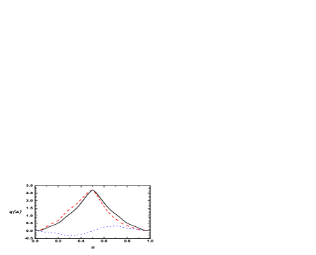
Figure 3: PDFs for S1 (left) and S2 (right). We have drawn the contribution from Eq. (2) ($q_{u}^{\left(1\right)}\left(x\right)$, dashed line), from Eq. (6) ($\tilde{q}_{u}^{\left(1\right)}\left(x\right)$, dotted line) and the total parton distribution (full line).

We have also looked to the behavior of the PDFs under variations of the parameters present in the expression of $m\left(p\right)$ and $Z\left(p\right)$. We observe that not all values of the parameters are permitted by our consistency requirements. For instance, if we increase $\alpha_{m}$ or $\alpha_{Z}$ by a factor 2 we observe that the second moment of the PDF deviates from 0.5 and the PDF is not more symmetric around the point $x=0.5.$ These results appear because the Wick rotation introduces spurious contributions. Let us be more precise, our formalism preserves all the symmetries up to the point in which we perform the Wick rotation. It is while performing the latter that, if “spurious” poles and/or cuts are close to the physical ones, appreciable errors might arise. The position of these singularities depends on the “models” and the “parameter choice” in those models.

Let us now change our parameters in the opposite direction in order to compare our approach with the NJL model. We multiply $\Lambda_{m}$ and $\Lambda_{Z}$ by 2, and at the same time divide $\alpha_{m}$ and $\alpha_{Z}$ by 2 to insure that the value of the physical observables, like the quark condensate, do not change too much. This change makes the currents in Eqs. (9) more point like, leading to a model whose results, in the limit $\alpha_{Z}\rightarrow 0,$ $\Lambda_{m}\rightarrow\infty$ resemble those of the NJL model. In Fig. 4 we show the pion PDF in S2, Eqs. (20) and (21), with the following changes: (i) $\Lambda_{Z}$ multiplied by 2 and $\alpha_{Z}$ divided by 2 (dashed line); (ii) $\Lambda_{m}$ multiplied by 2 and $\alpha_{m}$ divided by 2 (dotted line); (iii) both $\Lambda m$ and $\Lambda_{Z}$ multiplied by 2 and both $\alpha_{Z}$ and $\alpha_{m}$ divided by 2 (dashed-dotted line). We observe the similarity, especially of the last case, to the result of the NJL model in the chiral limit, $q\left(x\right)=1.$

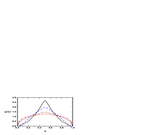
Figure 4: Full line corresponds to S2, Eqs. (20 ) and (21). The other curves corresponds to changes in the parameters of this scenario: (i) $\alpha_{Z}$ divided by 2 and $\Lambda_{Z}$ multiplied by 2 (dashed line); (ii) $\alpha_{m}$ divided by 2 and $\Lambda_{m}$ multiplied by 2 (dotted line); (iii) both $\alpha_{Z}$ and $\alpha_{m}$ divided by 2 and both $\Lambda_{m}$ and $\Lambda_{Z}$ multiplied by 2 (dashed-dotted line).

Some doubts maybe cast in our calculation having to do with the relation between the calculation in Minkowsky and Euclidean spaces, as a consequence of the singularity structure discussed in section II. In section IV we resolve this problem by calculating the moments of the parton distribution functions in three different ways and proving that for the scenarios described above the three methods fully agree.

By explicit construction, our quarks are constituent quarks. The experimental parton distributions however, unveil the structure of the pion in terms of fundamental partons. How to relate the constituent quarks and the fundamental partons is an old problem analyzed by Altarelli, Cabibbo, Maiani and Petronzio AltarelliCabibboMaianiPetronzio74 , and applied more recently to the pion AltarelliPetrarcaRapuano96 and to the nucleon Scopetta1 ; Scopetta2 . Let us recall the main features of this development.

As shown in ref.AltarelliCabibboMaianiPetronzio74 , the constituent quarks are themselves composite objects whose structure is described by a set of functions $\phi_{q_{0}q}\left(x\right)$ that specify the number of point-like partons of type $q$ which are present in the constituent of type $q_{0}$, with fraction $x$ of its total momentum. We will hereafter call these functions, generically, the structure functions of the constituent quark. The functions describing the nucleon parton distributions are expressed in terms of these new functions $\phi_{q_{0}q}\left(x\right)$ and of the calculated constituent density distributions $(q_{0}=u_{0},d_{0})$ as,

$$q\left(x,Q^{2}\right)=\sum_{q_{0}}\int_{x}^{1}\frac{dz}{z}\ q_{0}\left(z,Q^{2}\right)\ \phi_{q_{0}q}\left(\frac{x}{z},Q^{2}\right)$$ (22)

where $q$ labels the various partons, i.e., valence quarks and antiquarks $(u_{v},\bar{d}_{v})$, sea quarks $(u_{s},d_{s},s)$, sea antiquarks $\left(\bar{u}_{s},\bar{d}_{s},\bar{s}\right)$ and gluons $g.$

The different types and functional forms of the structure functions of the constituent quarks are derived from three very natural assumptions AltarelliCabibboMaianiPetronzio74 : (i) The point-like partons are QCD degrees of freedom, i.e. quarks, antiquarks and gluons; (ii) Regge behavior for $x\rightarrow 0$ and duality ideas; (iii) invariance under charge conjugation and isospin.

These considerations define in the case of the valence quarks the following structure function

$$\phi_{q_{0}q_{v}}\left(x,Q^{2}\right)=\frac{\Gamma\left(A+\frac{1}{2}\right)}{\Gamma\left(\frac{1}{2}\right)\Gamma\left(A\right)}\frac{\left(1-x\right)^{A-1}}{\sqrt{x}}\ .$$ (23)

For the sea quarks the corresponding structure function becomes,

$$\phi_{q_{0}q_{s}}\left(x,Q^{2}\right)=\frac{C}{x}\left(1-x\right)^{D-1}\ ,$$ (24)

and, in the case of the gluons, it is taken

$$\phi_{q_{0}g}\left(x,Q^{2}\right)=\frac{G}{x}\left(1-x\right)^{B-1}\ .$$ (25)

We take the same parameters as in ref.Scopetta1 for the proton case $A=0.435,$ $B=0.378,$  $C=0.05,$ $D=2.778,$ and $G=0.135$, since these functions should in principle be independent of the hadron under scrutiny.

Once the convolution defined by Altarelli et al. is performed, we proceed to look for the evolution of the parton distribution under the Renormalization Group. The evolution is carried to next to leading order. We find the hadronic scale, i.e. the scale at which the constituent quark structure is defined, at $Q_{0}^{2}=1\operatorname{GeV}^{2}$. This scale is determined by imposing that the fraction of the total momentum carried by the valence quark at $Q^{2}=4\operatorname{GeV}^{2}$ is 0.46 as determined from experiment SuttonMartinRobertsStirling92 .

In Fig. 5 we show the evolved PDF for S2 (full line). S1, discussed at the beginning of the section, gives similar results. The dashed line corresponds to the evolution of the PDF of S2 without the ACMP convolution. We observe that the results are reasonable since not a single parameter was fixed in the fit, although too small in the $x\sim 1$ region. The ACMP procedure pushes the PDF to higher values of $x$ and therefore produces a significant corrections in the right direction.

We show in Fig. 5 also the results obtained with S2 for $\Lambda_{m}$ and $\Lambda_{Z}$ multiplied by 2 and $\alpha_{Z}$ and $\alpha_{m}$ divided by 2 (dashed-dotted line). We observe that the experimental results are well reproduced in this case and our curve is very well reproduced by the expression

$$xq\left(x\right)=\frac{\Gamma\left(1+\alpha+\beta\right)}{\Gamma\left(\alpha\right)\Gamma\left(1+\beta\right)}x^{\alpha}\left(1-x\right)^{\beta}\qquad\text{with }\alpha=0.62,\beta=1.04$$ (26)

which is quite close to the bests fits in SuttonMartinRobertsStirling92 . The fact that the PDF in terms of the constituent quarks is larger in the regions $x\sim 0$ and $x\sim 1$ leads, after applying the ACMP procedure, to a result which is reasonable in the large $x$ region. The NJL model, when the ACMP procedure is applied to it, leads to a PDF which too large in the $x\sim 1$ region, although quite reasonable given the simplicity of the model and the fact that no single parameter was fitted in the process (small dashed line in Fig. 5).

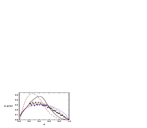
Figure 5: Full line corresponds to the evolved PDF for S2 including the ACMP procedure. The dashed line corresponds to the evolution of the PDF of the same scenario without the ACMP convolution. The dashed-dotted and small-dashed lines are for the evolved PDF for S2 with $\alpha_{Z}$ and $\alpha_{m}$ divided by 2 and $\Lambda_{m}$ and $\Lambda_{Z}$ multiplied by 2 and for the NJL model respectively, in both cases the ACMP procedure is implemented.

IV Moments of the constituent parton distribution functions.

In section II we have calculated the parton distribution $q\left(x\right).$ We have assumed that the parton distribution is defined between $0<x<1$ and have used as a consistency test of this assumption that the first moment of the parton distribution is $1$ and the second moment is $1/2$. From Eq. (2), (6) and (7)it can be analitically proved that

$$\begin{array}[c]{c}\int dx~{}q\left(x\right)=F\left(0\right)\;\;,\\ \int dx~{}x~{}q\left(x\right)=\frac{1}{2}F\left(0\right)\;\;,\end{array}$$ (27)

when the integration is not restricted to the region $0\leq x\leq 1$ . The consistency test proposed in section II reflects that the significant contribution to the two integrals (27) comes from the physical region $0\leq x\leq 1$.

The numerical value of the higher moments are not fixed by symmetry arguments. Nevertheless we can use them as a proof of the consistency of our procedure if we are able to calculate them in a different way. We proceed to do so.

The moments of the parton distribution are defined as:

$$\left\langle x\right\rangle_{s}=\int_{0}^{1}dx~{}x^{s-1}~{}q\left(x\right)$$ (28)

A first procedure to calculate the moments is to perform the integration defined in Eq. (28) using the parton distribution, $q\left(x\right),$ obtained in section II. An alternative method is to perform the integral over $x,$ using the delta functions present in Eqs. (2), (6) and (7), before performing the integration over the internal momentum, $p,$ in these equations. We focus our discussion in the contribution to $\left\langle x\right\rangle_{s}$ coming from (2), because the generalization to the other two contributions is straightforward.

Once the integral over $x$ is performed, the contribution to $\left\langle x\right\rangle_{s}$ coming from (2) is

$$\left\langle x_{1}\right\rangle_{s}=-\int\frac{d^{4}p}{\left(2\pi\right)^{4}}\text{ }\left[\frac{n}{2}\cdot\left(2p+P\right)\right]^{s-1}\,\mathbb{T}\mathrm{r}\left[i\,S\left(p-\frac{1}{2}P\right)\bar{\Gamma}^{M}\left(p,P\right)i\,S\left(p+\frac{1}{2}P\right)\right.$$

$$\left.\Gamma_{\mu}\left(p+\frac{1}{2}P,p+\frac{1}{2}P\right)n^{\mu}\,i\,S\left(p+\frac{1}{2}P\right)\Gamma^{M}\left(p,P\right)\right]$$ (29)

with the momentum integration restricted to those values that guaranty the condition

$$0<\frac{n}{2}\cdot\left(2p+P\right)<1\;\;.$$ (30)

The difference between the first and the second procedures is just the order of integration of the variables. Any significant problem with singularities must appear in comparing the result of these two methods.

For calculating the integral present in Eq. (29) we need a reference frame. The most adequate one is the infinite momentum frame, in which we have $n^{\mu}=\left(1,0,0,-1\right)/\sqrt{2}\bar{P}$ with $\bar{P}$ going to infinity. The pion momentum is expressed as

$$P^{\mu}=\frac{1}{\sqrt{2}}\left(\bar{P}+\frac{m_{\pi}^{2}}{2\bar{P}},0,0,\bar{P}-\frac{m_{\pi}^{2}}{2\bar{P}}\right).$$ (31)

In this reference frame the dominant terms appearing in the denominators of the propagators are proportional to $\bar{P},$ $[~{}\left(p\pm P/2\right)^{2}$ $\propto$ $\pm\frac{1}{\sqrt{2}}\left(p^{0}-p^{3}\right)\bar{P}~{}],$ which lead to an integrand vanishing as $\bar{P}^{-2}$ for large values of $\bar{P},$ except in a small region of $p^{0}$ around $p^{3}.$ In order to evaluate the contribution of this region it is adequate to make the following change of variable

$$p^{0}=p^{3}+\frac{\bar{m}}{\bar{P}}p^{\prime 0}$$ (32)

where $\bar{m}$ is any mass in the problem, for instance $\bar{m}=m\left(0\right).$

Using (32) in eq. (30) we obtain that the integration over $p^{3}$ must be performed between $-\bar{P}/(2\sqrt{2})$ and $\bar{P}/(2\sqrt{2})$ and similarly for $p^{0}$. Then, the contribution coming from (29) is

$$\left\langle x_{1}\right\rangle_{s}=-\lim_{\bar{P}\rightarrow\infty}\int_{-\bar{P}/(2\sqrt{2})}^{\bar{P}/(2\sqrt{2})}\frac{\bar{m}}{\bar{P}}\frac{dp^{\prime 0}}{2\pi}\int_{-\bar{P}/(2\sqrt{2})}^{\bar{P}/(2\sqrt{2})}\frac{dp^{3}}{2\pi}\int\frac{d^{2}p_{\bot}}{\left(2\pi\right)^{4}}\text{ }\left[\sqrt{2}\frac{p^{3}}{\bar{P}}+\frac{1}{2}\right]^{m-1}\,$$

$$\mathbb{T}\mathrm{r}\left[i\,S\left(p-\frac{1}{2}P\right)\bar{\Gamma}^{M}\left(p,P\right)i\,S\left(p+\frac{1}{2}P\right)\right.\left.\Gamma_{\mu}\left(p+\frac{1}{2}P,p+\frac{1}{2}P\right)n^{\mu}\,i\,S\left(p+\frac{1}{2}P\right)\Gamma^{M}\left(p,P\right)\right]$$ (33)

It is a this stage that we assume that the Wick rotation on the variable $p^{\prime 0}$ can be performed without problems. The most dangerous term, $\left[n\cdot\left(2p+P\right)/2\right]^{s-1},$ is under control for any value of $s$. It is not difficult to show that this integral has a well defined value as $\bar{P}\rightarrow\infty$ and that this value is independent of $\bar{m}$ in Eq.(32).

We have applied the same procedure to the other two contributions to $\left\langle x\right\rangle_{s},$ coming form Eqs. (6) and (7) and we have calculated the moments of the parton distribution in the two scenarios, S1 and S2, defined in section III. We have also calculated them directly from Eq. (28) with the parton distributions obtained in section III. The numerical results coincide in both scenarios for all the moments.

Summarizing, in here we have calculated the moments of the parton distribution functions for the two scenarios defined in section III in two different ways. Firstly, from Eq. (28) using the calculated parton distribution obtained from the method explained in section II. In this first method we do not need to define a particular frame for the calculation. In the second method, we have calculated the moments directly in Euclidean space and in the infinite momentum frame. This second procedure has been justified from an analysis in Minkowsky space, by performing the Wick rotation in Eq. (33) and the equivalent equations for the other two contributions coming from Eqs. (6) and (7). The methods are based on significantly different calculations and therefore, they provide a test of consistency. Those models which violate the check of consistency defined at the end of section II, will also give different numerical results for the moments of the parton distribution functions in the two methods.

V Conclusions.

We have applied a procedure for calculating the PDFs in a framework, based on the Dyson-Schwinger equations, first introduced in ref. Noguera05 . The motivation behind our procedure is the preservation of all the conservation laws associated with the fundamental symmetries (Poincaré covariance, gauge invariance, isospin symmetry and number of valence constituents) which implies that before evolution the PDF of the pion built with only two valence (anti)quarks has first moment equal to 1, second moment equal to 0.5, is symmetric around the point $x=0.5$ and is defined in $0<x<1.$ Our procedure, determined by the appropriate implementation of local gauge invariance, is defined in terms of an operator, which incorporates additional contributions besides the conventional triangle diagram Noguera05 . The method of calculation follows the method used in NogueraTheusslVento04 for the calculation of the GPDs in the NJL model and can be easily applied to any model with similar ingredients.

Our approach preserves all the symmetries up to the moment in which the Wick rotation is performed. The particular choice for $m\left(p\right)$ and $Z\left(p\right)$ becomes crucial at this moment. An arbitrary choice of $m\left(p\right)$ or $Z\left(p\right)$ can have “spurious” singularities which might lead to appreciable symmetry breaking effects. Our expressions for these functions, obtained from QCD studies, are consistent, within our numerical precision, with all the symmetries. Note the parton distribution vanishes at the support endpoints, $x=0$ and $x=1$, a feature which occurs in the instanton model PolyakovWeiss99 , but not in the NJL model. The new terms in the operator give no contribution to the first moment of the PDF, but a significant contribution ($\sim 6-8\%$) to the second moment and restore the symmetry of the PDF around the point $x=0.5$. We can approach the results of the NJL model by a change in the parameters.

In order to check furthermore our procedure we have calculated the moments of the parton distribution in two different ways. The consistency of these procedures provides a strong test for our formalism to determine the parton distributions.

In order to describe the experimental data we have realized that the ACMP procedure is necessary. Nevertheless, even incorporating the ACMP convolutions, the results with the given parameterization are not spectacular, they fall very low for large $x$. On the other hand, the NJL model, also with ACMP convolutions, behaves oppositely, its PDFs is too large in that region. Since we can approach the NJL model in our scheme by increasing $\Lambda_{m}$ we do so, changing simultaneously $\alpha_{m}$ to keep the low energy properties as close as possible to the experimental ones. The improvement is immediate although we have done no fine tuning. Nevertheless, we do not make a big statement about this improvement, since there might be other contributions to the PDFs arising from improvements to our lagrangian, which are lacking in our formulation.

Fundamental studies of QCD provide results which lead to effective nonlocal interactions which are difficult to connect with the data. The analysis carried out here shows that the formalism developed in ref.Noguera05 is well suited for this purpose. The formalism can be easily generalized to any model, is based on the Dyson-Schwinger equations, and therefore contains all the non perturbative input associated with the bound state structure of hadrons, and is suited to preserve all the wishful symmetries, as long as we are able to control the passage from Euclidean to Minkowski space-times. Besides these general conclusions, we have also shown, in the calculation of the PDFs, that the models thus far developed to describe the structure of hadrons at low $Q^{2}$ (scenarios S1 and S2) require from a convolution formalism of the ACMP type to approach the data. Moreover, surprisingly enough, without any change in the parameters of these models, the results, once ACMP is incorporated, are qualitatively correct. Finally, with little changes in the parameterization we have also shown that one can easily adjust both low energy and high energy observables within the same model lagrangian. We have not pretended to do so precisely, since our model is far too crude to be able to explain the data, but our calculations shows that this enterprise is feasible.

Appendix A Description of the quark propagator and pion amplitude.

In ref Noguera05 it is studied the model described by the lagrangian of Eq. (8). We obtain from the Dyson equation the momentum dependence of the mass and wave function renormalization of the propagator of Eq. (11):

$$m\left(p\right) =\frac{m_{0}+\alpha_{0}G_{0}\left(p\right)}{1-\alpha_{p}G_{p}\left(p\right)}$$ (34)

$$Z\left(p\right) =\frac{1}{1-\alpha_{p}G_{p}\left(p\right)}$$ (35)

The constants $\alpha_{0}$ and $\alpha_{p}$ are directly related to couplings constants $g_{0}$ and $g_{p}:$

$$\alpha_{0} =i\,8\,N_{c}N_{f}g_{0}\int\frac{d^{4}p}{\left(2\pi\right)^{4}}G_{0}\left(p\right)\frac{Z\left(p\right)m\left(p\right)}{p^{2}-m^{2}\left(p\right)+i\epsilon}$$ (36)

$$\alpha_{p} =i\,8\,N_{c}N_{f}g_{p}\int\frac{d^{4}p}{\left(2\pi\right)^{4}}G_{p}\left(p\right)\frac{p^{2}Z\left(p\right)}{p^{2}-m^{2}\left(p\right)+i\epsilon}$$ (37)

The BS equation is solved leading to:

$$\Gamma^{M=\pi^{i}}\left(p,P\right)=\,i\,\gamma_{5}\,\tau^{i}\,g_{\pi qq}G_{0}\left(p\right)$$ (38)

Defining the pseudo-scalar polarization

$$\Pi_{ps}\left(P^{2}\right)=-~{}i\,4\,N_{c}\,N_{f}\int\frac{d^{4}p}{\left(2\pi\right)^{4}}G_{0}^{2}\left(p\right)\frac{Z\left(p+\frac{1}{2}P\right)\,Z\left(p-\frac{1}{2}P\right)\left[\frac{1}{4}P^{2}-p^{2}+m\left(p+\frac{1}{2}P\right)m\left(p-\frac{1}{2}P\right)\right]}{\left[\left(p+\frac{1}{2}P\right)^{2}-m^{2}\left(p+\frac{1}{2}P\right)+i\epsilon\right]\left[\left(p-\frac{1}{2}P\right)^{2}-m^{2}\left(p-\frac{1}{2}P\right)+i\epsilon\right]}~{}~{},$$ (39)

the pion mass is obtained from the relation:

$$1=2\,g_{0}\,\Pi_{ps}\left(P^{2}=m_{\pi}^{2}\right)$$ (40)

and the normalization constant $g_{\pi qq}$ is given by

$$\frac{1}{g_{\pi qq}^{2}}=-\left(\frac{\partial\Pi_{ps}}{\partial P^{2}}\right)_{P^{2}=m_{\pi}^{2}}~{}.$$ (41)

References

- (1) D. Müller, D. Robaschick, B. Geyer, F.M. Dittes and J. Horejsi,Fortschr. Phys. 42, 101 (1994).
- (2) A.V. Radyushkin, Phys. Lett B380, 417 (1996), Phys. Lett B385, 333 (1996).
- (3) X.D. Ji, Phys. Rev. Lett. 78, 610 (1997), Phys. Rev. D55, 7114 (1997).
- (4) M. Diehl, Phys. Rep. 388, 41 (2003).
- (5) S. Noguera, hep-ph/0502171
- (6) J. Badier et al. NA3 Collaboration, Z. Phys. C18, 281 (1983)
- (7) B. Betev et al. NA10 Collaboration Z. Phys. C28, 15 (1985)
- (8) J. S. Conway et al Phys Rev D39, 92 (1989)
- (9) P. Aurenche et al. Phys. Lett. B233, 517 (1989)
- (10) P. J. Sutton, A. D. Martin, R. G. Roberts, W. J. Stirling, Phys. Rev. D45, 2349 (1992)
- (11) C. Best et al.Phys. Rev. D56, 2743 (1997).
- (12) W. Detmold, W. Melnichouk, A. W. Thomas, Phys. Rev. D68, 034025 (2003)
- (13) R. M. Davidson and E. Ruiz Arriola, Phys. Lett. B348, 163 (1995); Acta Phys. Pol. B33, 1791 (2002).
- (14) F. Bissey, J.R. Cudell, J. Cugnon, J.P. Lansberg, P. Stassart, Phys.Lett. B587, 189 (2004); F. Bissey, J.R. Cudell, J. Cugnon, M. Jaminon, J.P. Lansberg, P. Stassart, Phys.Lett. B547 210 (2002).
- (15) E. Ruiz Arriola and W. Broniowski, Phys. Rev. D66, 094016 (2002).
- (16) S. Noguera, L. Theußl and V. Vento Eur.Phys.J. A20, 483 (2004).
- (17) Y. Nambu and G. Jona-Lasinio, Phys. Rev. 124, 246 (1961).
- (18) E. Ruiz Arriola and W. Broniowski, Phys. Rev. D 67, 074021 (2003).
- (19) M. V. Polyakov and C. Weiss, Phys. Rev. D60, 114017 (1999)
- (20) M. V. Polyakov Nucl. Phys. B555, 231 (1999)
- (21) M. Alberg and E. M. Henley, Phys. Lett. B611, 111 (2005)
- (22) I.V. Anikin, D. Binosi, R. Medrano, S. Noguera, V. Vento Eur.Phys.J.A14, 95 (2002).
- (23) B. C. Tiburzi and G. Miller, Phys. Rev. C64, 065204 (2001); Phys. Rev. D65, 074009 (2002); Phys. Rev. D67, 113004 (2003). B. C. Tiburzi Ph. D. Thesis nucl-th/0407005
- (24) S. Simula hep-ph/0406074
- (25) M. B. Hecht, C. D. Roberts and S. M. Schmidt, Phys. Rev. C63, 025213 (2001).
- (26) M. Traini, V. Vento, A. Mair, A. Zambarda, Nucl. Phys. A614, 472 (1997).
- (27) G. Altarelli, N. Cabibbo, L. Maiani, R. Petronzio, Nucl. Phys. B69, 531 (1974).
- (28) S. Scopetta, V. Vento, M. Traini, Phys. Lett. B421, 64 (1998); Phys. Lett. B442, 28 (1998).
- (29) S. Scopetta, V. Vento, Phys. Rev. D69, 094004 (2004); Phys.Rev. D71, 014014 (2005).
- (30) G. Altarelli, S. Petrarca, F. Rapuano, Phys. Lett. B373, 200 (1996).
- (31) S. Noguera, S. Scopetta, V. Vento, Phys. Rev. D70, 094018 (2004).
- (32) J.S. Ball and T.W. Chiu, Phys. Rev. D22, 2542 (1980).
- (33) D.C. Curtis and M.R. Pennington, Phys. Rev. D42, 4165 (1990).
- (34) C. D. Roberts, Nucl. Phys. A605, 475 (1996).
- (35) A. Bender, W. Detmold, A. W. Thomas , C.D. Roberts, Phys.Rev. C65, 065203, (2002).
- (36) D. I. Dyakonov and V. Yu. Petrov, Nucl. Phys. B272, 457 (1986).
- (37) P. O. Bowman, U. M. Heller and A. G. Williams, Phys. Rev. D66, 014505 (2002) .
- (38) P. O. Bowman, U. M. Heller, D. B. Leinweber and A. G. Williams, Nucl.Phys.Proc.Suppl.119, 323 (2003).
- (39) C. J. Burden, C. D. Roberts and A. G. Williams, Phys. Lett. B285, 347 (1992).
- (40) H. J. Munczek and A. M. Nemirovsky, Phys. Rev. D 28, 181 (1983).
- (41) F. T. Hawes, C. D. Roberts and A. G. Williams, Phys. Rev. D 49, 4683 (1994).