The high energy asymptotics of scattering processes in QCD

Abstract

High energy scattering in the QCD parton model was recently shown to be a reaction-diffusion process and, thus, to lie in the universality class of the stochastic Fisher-Kolmogorov-Petrovsky-Piscounov equation. We recall that the latter appears naturally in the context of the parton model. We provide a thorough numerical analysis of the mean field approximation, given in QCD by the Balitsky-Kovchegov equation. In the framework of a simple stochastic toy model that captures the relevant features of QCD, we discuss and illustrate the universal properties of such stochastic models. We investigate, in particular, the validity of the mean field approximation and how it is broken by fluctuations. We find that the mean field approximation is a good approximation in the initial stages of the evolution in rapidity.

I Introduction

The description of the rise of hadronic cross sections with the center of mass energy $\sqrt{s}$ within quantum chromodynamics (QCD) has been a challenging issue. Old experimental results, e.g. on proton scattering, do not yet have a satisfactory theoretical explanation. So far, no realization has been found for the Froissart bound, which is a consequence of the unitarity of the $S$-matrix and which is a bound on the high energy behavior of the total cross sections, $\sigma\leq(1/m_{\pi}^{2})\ln^{2}s$.

A perturbative calculation of the evolution of scattering amplitudes with energy, achieved by Balitsky, Fadin, Kuraev and Lipatov (BFKL) 30 years ago BFKL and subsequently improved to next-to-leading order NLBFKL , is apparently successful in describing the rise of photon-proton cross sections when the virtuality of the photon is high enough. However, the BFKL equation, being linear, is not compatible with the Froissart bound when it is extrapolated to very high energies. Complying with the limits set by unitarity requires the introduction of nonlinear terms in the evolution equations. A first step in this direction was taken by Gribov, Levin and Ryskin (GLR) in 1981 GLR , and by Mueller and Qiu (MQ) in 1986 MQ . Subsequently, more involved QCD evolution equations were derived within different formalisms. Balitsky, Jalilian-Marian, Iancu, McLerran, Weigert, Leonidov and Kovner (B-JIMWLK) B ; JIMWLK have developed a comprehensive approach to high energy scattering from different but converging points of view. Technically, they were able to write the high energy evolution of QCD amplitudes in the form of a functional integro-differential equation, that can also be expressed as a Langevin equation or as an infinite hierarchy of coupled differential equations. A much simpler equation was obtained by Balitsky B and by Kovchegov K (BK) in the particular physical context where the target is a large nucleus. The latter turns out to be a specific limit of the former, and its structure is similar to the GLR-MQ equation.

Meanwhile, on the phenomenological side, Golec-Biernat and Wüsthoff showed GBW that unitarization effects, that cannot be taken into account by a linear evolution such as the BFKL equation, may have already be seen at the DESY electron-proton collider HERA. Their observation gave a new impetus to the field and triggered many phenomenological and theoretical studies. Furthermore, the model they had proposed pointed towards a new scaling, “geometric scaling”, which was subsequently found in the HERA data SGK .

Much insight and intuition has been gained from numerical studies: even before the B-JIMWLK formalism had been developed, Salam performed numerical calculations of scattering amplitudes near the unitarity limits in the framework of a Monte-Carlo implementation Salam of Mueller’s color dipole model CD . More recently, much effort has been devoted to obtaining numerical solutions of the BK and B-JIMWLK equations AB ; L2001 ; GMS ; AAMSW ; RW , and in particular to the understanding of geometric scaling. But no analytical solution could be found.

Important progress was accomplished when the first terms of the large rapidity asymptotic expansion of the solutions to the Balitsky-Kovchegov equation were computed by Mueller and Triantafyllopoulos MT . This expansion was subsequently systematized with the discovery MP2003 ; MP2004 that the BK equation lies in the universality class of the Fisher-Kolmogorov-Petrovsky-Piscounov (FKPP) equation FKPP ; VS , and that geometric scaling was equivalent to the property that the latter admits traveling wave solutions. The FKPP equation describes a vast class of physical phenomena, actively studied by mathematicians and statistical physicists.

Meanwhile, Mueller and Shoshi MS made a first step in going beyond the BK approximation to high energy scattering in QCD. Through a sophisticated analysis of the unitarity and symmetry constraints on the QCD evolution, they were able to propose a correction to the saturation scale, induced by effects neglected in the BK evolution, and realized that geometric scaling was asymptotically broken.

The complete equivalence between high energy QCD and statistical physics models of reaction-diffusion type, first understood by one of us (S.M.) M2005 ; IMM , provided a new picture in which the nature of the effects neglected by the BK equation became transparent. The universality class of high energy QCD was identified as that of the stochastic Fisher-Kolmogorov-Petrovsky-Piscounov (sFKPP) equation Panja . The latter applies to a very wide class of physical phenomena, ranging from directed percolation to population growth. It has many applications, e.g. to biology, genetics, anthropology, fluid mechanics. Roughly speaking, most of the physical situations in which objects evolve by multiplying and diffusing, up to a certain limiting threshold, may be captured by an equation in the universality class of the sFKPP equation.

The crucial point is that the QCD parton model has such dynamics, when viewed in a particular way that we will explain in this paper. Once this observation is made, all mathematical results can be transposed to the physical context of high energy QCD IMM . In particular, Mueller and Shoshi’s results on the saturation scale are recovered. The breaking of geometric scaling, that they had understood qualitatively in their approach, is shown to be related to the statistical dispersion in the occupation numbers of partons in the hadronic Fock state. This new point of view on high energy QCD not only confirmed and brought new exact results on QCD scattering amplitudes: it also provided a physical understanding of the very nature and the role of fluctuations contained in the QCD evolution equations. Moreover, it helped to understand how to set up a systematics to go beyond the BK equation. It was recognized that the B-JIMWLK formalism was not complete IT ; MSW , thus confirming what was expected K ; KMW ; KL . The form of the new terms can be written down taking advantage of the correspondence to statistical physics.

The goal of this paper is to provide numerical solutions of the evolution equations of QCD, in order to study accurately their universal properties. The outline goes as follows: in Sec. II, we explain how the parton model is related to a reaction-diffusion process. ¿From physical but rigorous arguments, we derive in a simple way the evolution of the parton densities with energy, reviewing and expanding upon Refs. M2005 ; IMM . In particular, we show how the sFKPP equation appears. In Sec. III, we study numerically in detail a useful mean field approximation to the full evolution equations—that is, the BK equation—in relation to the most recent analytical results. In the final Sec. IV, we go beyond, investigating in a toy model the full content of the sFKPP equation and its consequences in QCD.

II Unitary evolution of amplitudes in the parton model

In this first section, we recall the physical picture of high energy scattering in the parton model (Sec. II.1) insisting on the manifest link to reaction-diffusion models. In a second step (Sec. II.2), following Ref. IMM , we derive the general evolution equations in QCD.

II.1 High energy scattering as a reaction-diffusion process

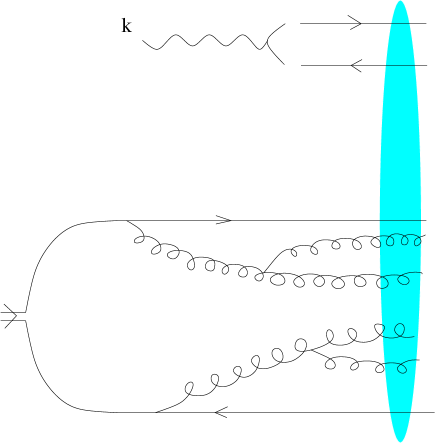
Figure 1: The scattering of a probe (here, a virtual photon characterized by the momentum scale $k$ interacting through its $q\bar{q}$ Fock state) off a particular 4-gluon fluctuation of the target dipole.

Let us consider the scattering of a hadronic probe off a given target, in the rest frame of the probe and at a fixed impact parameter. In the parton model, the target interacts through one of its quantum fluctuations (see Fig. 1). The probe effectively “counts” the partons in the current Fock state of the target whose transverse momenta $k$ match the one of the probe: the amplitude $T(k)$ for the scattering off this particular partonic configuration is proportional to the number of partons $n(k)$.

In QCD, the wave function of a hadronic object is built up from successive splittings of partons starting from the valence structure. As one increases the rapidity $Y$ by boosting the target, the opening of the phase space for parton splittings makes the probability for high occupation numbers larger. In the initial stages of the evolution, the parton density grows diffusively from these splittings.

On the other hand, the number of partons in each cell of transverse phase space is effectively limited to a maximum number $N$ that depends on the strength of the interaction of the probe with the partons, that is on the relationship between $T$ and $n$. This property is necessary from unitarity, which imposes an upper bound on the amplitude (e.g. $T(k)\leq 1$ with standard normalizations) which, in turn, results in an upper bound on $n(k)$. This is parton saturation and is realized by a recombination process.

Viewed in this way, scattering in the parton model is a reaction-diffusion process. The rapidity evolution of the Fock states of the target hadron is like the time evolution of a set of particles that diffuse in space, multiply and recombine so that there is no more than $N$ particles on each site, on the average. We parametrize space by the variable $x$: it will be related to $k$ in QCD. The QCD amplitude $T$ is like the fractional occupation number $u=n/N$ in the reaction-diffusion model.

In the continuum limit, it is known on general grounds DP that, up to a change of variable, $u$ obeys the evolution equation

$$\partial_{t}u(x,t)=D\partial_{x}^{2}u(x,t)+\lambda u(x,t)-\mu u^{2}(x,t)+\frac{1}{\sqrt{N}}\sqrt{2u(x,t)}\,\eta(x,t)\ ,$$ (1)

where $\eta$ is a Gaussian white noise, that is, a random function satisfying

$$\langle\eta(x,t)\rangle=0\ \ \ \mbox{and}\ \ \ \langle\eta(x,t)\eta(y,t^{\prime})\rangle=\delta(t-t^{\prime})\delta(x-y)\ .$$ (2)

Eq. (1) is known as the “Reggeon field theory” equation. It is to be interpreted in the standard Itō way, as the continuum limit of a discretized equation. It belongs to the same universality class as the stochastic Fisher-Kolmogorov-Petrovsky-Piscounov (sFKPP) equation (which may be obtained by the replacement $\sqrt{u}\rightarrow\sqrt{u(1-u)}$ in Eq. (1)). $D$ and $\lambda$ are parameters that characterize the diffusive growth of the particles. The structure of Eq. (1) is very transparent: the first two terms represent the growing diffusion of the particles, characterized by the parameters $D$ and $\lambda$, the third term implements the recombination process and tames this growth when maximum occupancy is approached. The last term results from the stochastic dynamics, whose effect reflects the finiteness of the number of particles. Note that this term gives rise to fluctuations in $u(x,t)$ and, consequently, in the particle number $n$, that are proportional to $\delta n\propto\sqrt{n}$. This is typical of fluctuations of independent random numbers, and reflects well the statistical origin of this term.

We do not mean that Eq. (1) fully represents parton evolution. Indeed, in the parton model, we anticipate that the rapidity evolution of parton densities be given, in the linear regime, by the BFKL equation, which is more complicated than a second order differential operator. But what we mean is that Eq. (1) describes exactly the critical behavior of the QCD amplitude $T\ (\sim u)$, that is its large rapidity (time) and large maximum occupancy number $N$ limit, up to the replacement of the relevant parameters.

All higher order operators beyond the ones appearing in Eq. (1) are irrelevant in these limits. As for the linear part, this is clear: the large time behavior stems from a saddle point that selects the quadratic approximation to the growing diffusion kernel. As a matter of fact, any equation of the form

$$\partial_{t}u(x,t)=K\otimes u(x,t)-\mu u^{2}(x,t)+\frac{1}{\sqrt{N}}\sqrt{2u(x,t)}\,\eta(x,t)\ ,$$ (3)

where $K$ is an appropriate differential or integral kernel encoding the growing diffusion, is believed to belong to that universality class and hence to exhibit the same asymptotic solutions. By “appropriate” we mean in practice that the phase velocity

$$v(\gamma)=\frac{K(\gamma)}{\gamma},\ \ \mbox{with}\ \ K(\gamma)=e^{\gamma x}(K\otimes e^{-\gamma x})$$ (4)

of a wave of wave number $\gamma$ propagated by the linear part of Eq. (3), must be a function of $\gamma$ that has a minimum in its domain of analyticity, but we should also stress that a general mathematical definition of the universality class of the Reggeon field equation is still not available Panja . As for the nonlinear part in Eqs. (1) and (3), terms of the form $u^{j}$ for $j>2$ would have no influence because the region $u\sim 1$ in which these terms show up is absorptive VS . Furthermore, we will see that the time evolution is essentially driven by the region where $u$ is small. Thanks to this property, we will not have to bother about the exact way how parton saturation actually occurs in QCD: it is enough to know that there is an upper bound on the number of partons by unit of transverse phase space.

So far, we have focused on the evolution of one (partonic) realization, described by Eq. (3). In the QCD context, $u\sim T$ represents the scattering amplitude off one particular Fock state. It is not a physical observable because it is not possible to select a particular Fock state of the target in a particle physics experiment. The physical amplitude that is measured in an experiment is the average over all accessible random (partonic) realizations. Only a few moments of $T$ may be measurable: its average, related to total cross sections, and its variance, related to diffractive cross sections, namely:

$$\begin{split}\sigma_{tot}&\sim\langle T\rangle\\ \sigma_{diff}&\sim\langle T^{2}\rangle-\langle T\rangle^{2}\ .\end{split}$$ (5)

The evolution of the moments of $T$ (or of $u$) may be computed directly from Eq. (1) (or Eq. (3)). Taking the average of Eq. (3), with the help of Eq. (2), it is straightforward to obtain the evolution of the latter

$$\partial_{t}\langle u(x,t)\rangle=K\otimes\langle u(x,t)\rangle-\mu\langle u^{2}(x,t)\rangle\ .$$ (6a)

However, this equation is not closed: it calls for an evolution equation for the correlator $$\langle u^{2}(x,t)\rangle$$, that can be derived again from Eq. (3) with the help of Eq. (2):

$$\partial_{t}\langle u(x,t)u(y,t)\rangle=(K_{x}+K_{y})\otimes\langle u(x,t)u(y,t)\rangle-\mu\langle u^{2}(x,t)u(y,t)\rangle-\mu\langle u(x,t)u^{2}(y,t)\rangle+\frac{2}{N}\delta(x\!-\!y)\langle u(x,t)\rangle\ ,$$ (6b)

and so on for the higher order correlators, leading eventually to an infinite hierarchy of coupled equations.

Note that the hierarchical form (6) was proposed by Parisi and Zhang Parisi to describe a growth process known as the Eden model. In the same paper, they also obtained the same hierarchy from the Reggeon action, which had already been proved to be related to stochastic processes ACMP_GS . Only the boundary terms (last term in the right-hand side of Eq. (6b)) could not be obtained from the Reggeon action through the Parisi-Zhang procedure: indeed, they refer explicitly to the way one counts the objects, as can be seen from the fact that this term is proportional to $2/N$, and the knowledge of the evolution encoded in the bulk terms of the action they had used is not enough.

Due to universality of the asymptotics of reaction-diffusion processes, it is straightforward to take over Eq. (3) or equivalently Eqs. (6a) and (6b) (and the higher equations in this hierarchy), together with their exact asymptotic solutions that will be exhibited in the following sections, to describe high energy QCD. Basically, an elementary analysis of the parton splitting process and how the partons interact perturbatively with a probe will be enough. This will enable us to identify the variables $t$ and $x$, the kernel of the linear evolution $K$ and the strength of the noise $1/N$ that correspond to the QCD parton model. We will turn to this analysis in the next section.

For Eq. (3), being both explicitly nonlinear and stochastic, it proves a formidable task to find solutions. However, there has been much progress recently in this direction Panja . It was realized that, starting from a localized initial condition, the large time solution is a traveling wave moving in the direction of larger $x$, up to some noise. The position $X_{t}$ of that wave may be defined in several ways. For example, one can pick a constant $\kappa$, and define $X_{t}$ in such a way that

$$u(X_{t},t)=\kappa\ .$$ (7)

An alternative definition, useful in particular in the case of discrete models, could be

$$X_{t}=\int_{0}^{\infty}dx\,u(x,t)\ .$$ (8)

In the context of QCD, $X_{t}$ is related to the saturation scale, that is, the point at which parton saturation effects set in.

Outstanding results have been obtained on $X_{t}$ and on the profile of the wave front $u(x,t)$ in the region $1/N\ll u\ll 1$. An interesting point is that the analytical formulas depend only on some local properties of the characteristic function $K(\gamma)$ of the linear diffusion kernel.

II.2 The evolution equations of the QCD parton model

In this section, we review the discussion of Ref. IMM . Our goal is to identify the relevant variables $t$, $x$, $N$ and the evolution kernel $K$ that correspond to the physical situation of QCD.

We consider the scattering of a dipole of variable size $r$ (the probe) off a dipole of size $r_{0}$ (the target). A natural variable that will be used throughout is $\rho\!=\!\ln(r_{0}^{2}/r^{2})$. We go to the rest frame of the probe so that the target carries all the available rapidity $Y$. The impact parameter $b$ between the dipoles is fixed.

At high energy, the quantum fluctuations of the target that interact with the probe are dominated by gluons. It proves useful to represent this set of partons by color dipoles CD . This is possible in the large-$N_{c}$ limit, where gluons are similar to zero-size $q\bar{q}$ pairs and non-planar diagrams are suppressed. Subleading-$N_{c}$ terms do not contribute to the evolution of the scattering amplitudes when they are small. However, the dipole approximation breaks down when the amplitudes approach their unitarity limits at the same time as nonlinearities set in, but as we will see, that does not hamper getting the right asymptotics for the physical quantities that we are going to compute.

We denote by $T(r,Y)$ the scattering amplitude of the probe off a given partonic realization $|\omega\rangle$ of the target, obtained after a rapidity evolution $Y$ (the dependence on $b$ is understood). It is a random variable, whose probability distribution is related to the distribution of the different Fock state realizations of the target. The values of $T(r,Y)$ range between 0 (weak interaction) and 1 (unitarity limit). $T(r,Y)$ will be an essential intermediate quantity in our calculations, but as has been explained in Sec. II.1, it is not an observable. The physical dipole-dipole scattering amplitude $A(r,Y)$ is the statistical average over all partonic fluctuations of the target at rapidity $Y$, i.e.

$$A(r,Y)=\langle T(r,Y)\rangle;$$ (9)

see Eq. (5).

When $T$ is small, the scattering amplitude off one particular Fock state $\omega(Y)$ is the sum of all elementary amplitudes with each of the dipoles, i.e.

$$T(r,Y)=\sum_{i\in\omega(Y)}T_{el}(r,r_{i})\ ,$$ (10)

where $i$ labels the dipoles in the Fock state of the target at the time of the interaction. $T_{el}$ is the elementary dipole interaction and is essentially local in impact parameter. $T_{el}$ behaves like

$$T_{el}(r,r_{i})\sim\alpha_{s}^{2}\,\frac{r_{<}^{2}}{r_{>}^{2}}\ ,\ \mbox{with}\ r_{<}=\min(|r|,|r_{i}|)\ ,\ r_{>}=\max(|r|,|r_{i}|)$$ (11)

when the dipoles overlap, and vanishes otherwise. We have neglected ${\mathcal{O}}(1)$ factors and logarithms, but these approximations do not affect the results that we shall obtain, which are largely independent of the details. Eq. (11) shows that the amplitude $T(r,Y)$ is simply counting the number $n(r,Y)$ of dipoles of size $r$ within a disk of radius $r$ centered at the impact parameter of the external dipole:

$$T(r,Y)\sim\alpha_{s}^{2}\,n(r,Y)\ .$$ (12)

Note that $n(r,Y)$ can take only discrete values: Indeed, it represents the number of quanta of a particular realization of the field of the target. The unitarity bound on $T$ implies that $n(r,Y)$ is also constrained by an upper bound $N\equiv 1/\alpha_{s}^{2}$. Later on, we shall switch to momentum space by the Fourier transformation $r\leftrightarrow k$. Of course, the relationship (12) will also hold for the Fourier conjugates.

We emphasize that the relationship (12) is only valid within the framework of the above-mentioned approximations. A more accurate treatment of how the counting of the partons is actually realized in QCD would eventually lead to more complex equations, see Ref. MSW . We will not enter these complications in this paper since we are only interested in the study of the asymptotics that are common with models from statistical physics, for which the counting rule (12) is precise enough.

The rapidity evolution law for $\langle T(r,Y)\rangle$ is known and we refer the reader to earlier literature for its derivation (e.g. IMM ). It reads

$$\partial_{Y}\langle T(r,Y)\rangle=\frac{\bar{\alpha}}{2\pi}\int d^{2}z\frac{r^{2}}{z^{2}(r\!-\!z)^{2}}(\langle T(z,Y)\rangle+\langle T(r\!-\!z,Y)\rangle-\langle T(r,Y)\rangle-\langle T(z,Y)T(r\!-\!z,Y)\rangle)\ .$$ (13a)

Eq. (13a) is not a closed equation for $$\langle T\rangle \langle T(z,Y)T(r\!-\!z,Y)\rangle \langle T(r_{1},Y)T(r_{2},Y)\rangle$$: It depends upon the correlator . An evolution equation for may be derived in the same way. One gets

$$\partial_{Y}\langle T(r_{1},Y)T(r_{2},Y)\rangle=\frac{\bar{\alpha}}{2\pi}\int d^{2}z\frac{r_{1}^{2}}{z^{2}(r_{1}\!-\!z)^{2}}(\langle T(z,Y)T(r_{2},Y)\rangle+\langle T(r_{1}\!-\!z,Y)T(r_{2},Y)\rangle-\langle T(r_{1},Y)T(r_{2},Y)\rangle\\ -\langle T(z,Y)T(r_{1}\!-\!z,Y)T(r_{2},Y)\rangle)\\ +\frac{\bar{\alpha}}{2\pi}\int d^{2}z\frac{r_{2}^{2}}{z^{2}(r_{2}\!-\!z)^{2}}(\langle T(r_{1},Y)T(z,Y)\rangle+\langle T(r_{1},Y)T(r_{2}\!-\!z,Y)\rangle-\langle T(r_{1},Y)T(r_{2},Y)\rangle\\ -\langle T(r_{1},Y)T(z,Y)T(r_{2}\!-\!z,Y)\rangle)\ ,$$ (13b)

which again calls for equations for higher correlators. Eqs. (13) turn out to be the first two parts of an infinite hierarchy originally derived by Balitsky B , restricted to dipoles.

In order to make the correspondence with reaction-diffusion models more concrete at the physical level, it is useful at this point to discuss qualitatively the typical shape of $T(r,Y)$ from the evolution. (The reader may find the complete derivation in Ref. IMM .) As one takes a new step in rapidity, each of the dipoles $r_{i}$ already present in the wave function from the previous step and for which $T(r_{i},Y)\ll 1$ may split into two new dipoles. The most probable splittings are those in which both child dipoles have a size comparable to the size of the parent dipole: they occur with probability one in each interval $\Delta Y\sim 1/\bar{\alpha}$. Thus the main mechanism for the rise of $T(r_{i},Y)$ with $Y$ is a growing diffusion around the size of the initial dipole $r_{i}$, that is encoded in the linear part of Eqs. (13). The nonlinear terms appearing therein tame this growth in order to satisfy the unitarity limits on $\langle T\rangle$.

In a typical partonic configuration as obtained after a sufficiently large rapidity evolution, the dipoles appear to be densely distributed around the size $r_{0}$ ($T(r,Y)$ is large), but they become more rare with decreasing $r$ (or increasing $\rho$), and for sufficiently large $\rho$ one meets only rare fluctuations which involve one (or few) dipoles and for which $T(r)\simeq\alpha_{s}^{2}$. It is a wave front which with increasing $Y$ progresses towards larger values of $\rho$. The position of that front is characterized by a momentum scale $Q_{s}(Y)$ called the saturation momentum. It is natural to define it e.g. by the value of the inverse dipole size for which the amplitude reaches some predefined number $\kappa$, i.e. $T(r\!=\!1/Q_{s}(Y),Y)=\kappa$: this corresponds to prescription (7).

We now proceed to the identification of the QCD evolution equation to the Reggeon field theory equation at the technical level. Following Ref. K , we perform the transformation

$$T(k,Y)=\int_{0}^{\infty}\frac{dr}{r}J_{0}(kr)T(r,Y)$$ (14)

to momentum space. The main positive outcome of such a transformation is to make the nonlinear terms in Eqs. (13) local in $k$, while obviously the linear part stays an integral kernel. It leads to the formal simplification

$$\left\{\begin{aligned} \partial_{\bar{\alpha}Y}\langle T(k,Y)\rangle&=\chi(-\partial_{L})\langle T(k,Y)\rangle-\langle T^{2}(k,Y)\rangle\\ \partial_{\bar{\alpha}Y}\langle T(k_{1},Y)T(k_{2},Y)\rangle&=(\chi(-\partial_{L_{1}})+\chi(-\partial_{L_{2}}))\langle T(k_{1},Y)T(k_{2},Y)\rangle\\ &\phantom{TTT}-\langle T^{2}(k_{1},Y)T(k_{2},Y)\rangle-\langle T(k_{1},Y)T^{2}(k_{2},Y)\rangle\\ &\cdots\end{aligned}\right.$$ (15)

where $L\equiv\ln(k^{2}/\Lambda^{2})$ and $\chi(\gamma)=2\psi(1)-\psi(\gamma)-\psi(1\!-\!\gamma)$ is the eigenvalue of the BFKL kernel. By $\chi\left(-\partial_{L}\right)$, we mean the BFKL integro-differential operator that may be defined with the help of the formal series expansion

$$\chi\left(-\partial_{L}\right)=\chi(\gamma_{0}){\mathbbm{1}}+\chi^{\prime}(\gamma_{0})(-\partial_{L}-\gamma_{0}{\mathbbm{1}})+{\scriptstyle\frac{1}{2}}\chi^{\prime\prime}(\gamma_{0})(-\partial_{L}-\gamma_{0}{\mathbbm{1}})^{2}+\cdots$$ (16)

for some given $\gamma_{0}$ between 0 and 1, i.e. for the principal branch of the function $\chi$.

It is clear that, as it stands, the hierarchy (15) admits the factorized “mean field” solution trivsol

$$\langle T(k_{1},Y)\cdots T(k_{n},Y)\rangle=\lambda^{n-1}\langle T(k_{1},Y)\rangle\cdots\langle T(k_{n},Y)\rangle$$ (17)

where $\lambda$ is any constant. However, this is not the physical solution that corresponds to scattering in QCD. The set of equations (15) may be supplemented by boundary terms if one wants to represent explicitly the elementary dipole interaction (i.e. the “counting rule”), which is absent in Eq. (15) (compare to Eq. (6b)). By analogy with statistical mechanics (see Eq. (6b)), this term should be Parisi

$$2\alpha_{s}^{2}\delta(L_{1}-L_{2})\langle T(k_{1},Y)\rangle$$ (18)

in the second equation. With this term, it is clear that (17) does no longer solve the hierarchy. Our method of derivation does not allow to find directly this boundary term, exactly for the same reasons Parisi and Zhang did not get it in their derivation of the hierarchy from the Reggeon action Parisi . Eq. (18) is nonzero when the transverse momenta of the two dipoles in the Fock space of the probe are equal, and thus, may scatter off the same dipole in the Fock space of the target: This was neglected in our derivation and has to be reintroduced by hand.

The evolution equation for $T$ may also be written in the form of a stochastic differential equation, namely,

$$\partial_{\bar{\alpha}Y}T(k,Y)=\chi(-\partial_{L})T(k,Y)-T^{2}(k,Y)+\alpha_{s}\sqrt{2T(k,Y)}\eta(k,Y)$$ (19)

that gives back the hierarchy (15) for the correlators, supplemented with boundary terms such as (18). Such a form was proposed for the first time in Refs. M2005 on physical grounds: Indeed, this is the universal asymptotic form of the evolution of any reaction-diffusion type process DP . Subsequently, it was shown on the technical level how the B-JIMWLK formalism can be made consistent with these physics IT ; MSW , and how this term may describe Pomeron loops (see also Refs. Lpomeronloop ). The source term (18) corresponds exactly to the one found there.

The identification with the Reggeon field theory equation is now straightforward:

$$\begin{split}x&\rightarrow L\ ,\ \ t\rightarrow\bar{\alpha}Y\ ,\\ K&\rightarrow\chi(-\partial_{L})\ ,\ \ \mu\rightarrow 1\ ,\\ N&\rightarrow 1/\alpha_{s}^{2}\ .\end{split}$$ (20)

Let us discuss the validity of Eq. (19) when applied to high energy scattering, and the physical expectations. As stated before, it is not expected to be exact, but we believe that it captures the essential physics of the QCD parton model. Since the linear part drives the front propagation at high rapidity, and since it is taken exactly into account here (to leading order in $\bar{\alpha}_{s}Y$), we expect that the solutions to this equation match the asymptotics of full QCD as far as the position of the front is concerned. This means that one should be able to get the asymptotics of the moments of the saturation scale $Q_{s}$ for $Y$ large, $\alpha_{s}\rightarrow 0$, and at a fixed impact parameter by solving (19). The latter limitations are necessary for the counting rule (12) to be valid. Similarly, the shape of $T$ in the region $1/N\ll T\ll 1$ is known to be universal and hence should also be obtainable from Eq. (19).

Of course, strictly speaking, these statements have the status of a conjecture, that will have to be confirmed by accurate numerical calculations, and in the long term, by a better mathematical understanding of the solutions of equations of the form (19).

There is still some important difference between the original Reggeon field theory equation (1) and the equation that we have obtained for high energy QCD. Indeed, $T(k,Y)=1$ is not a fixed point of the QCD evolution, unlike the case of the original Reggeon field theory equation, so the solutions cannot match in that region. Actually, it is known that $T(k,Y)\sim\ln(Q_{s}^{2}/k^{2})$ in the region $T\geq 1$ KL2005 . But anyway, we would not solve Eq. (19) around $T\geq 1$ because in the QCD case, the nonlinearity cannot be reduced to a simple quadratic term as in  (19), since also color structures beyond dipoles are expected to play a role there KL . That does presumably not influence the asymptotic saturation scale, which is completely determined by the linear part of the evolution equation, but it certainly modifies the shape of $T$ and of its correlators close to the unitarity limits.

III The mean field picture

The mean field approximation $\langle T^{2}(k,Y)\rangle\simeq\langle T(k,Y)\rangle^{2}\equiv A^{2}(k,Y)$ casts Eq. (13) into a closed form, known as the Balitsky-Kovchegov (BK) equation B ; K :

$${\partial_{\bar{\alpha}Y}}{A(k,Y)}=\chi\left(-\partial_{L}\right){A(k,Y)}-{A^{2}(k,Y)}\ .$$ (21)

A priori, the validity condition for such an approximation is not clear. We will be able to assess it only by studying the full problem including fluctuations. It is nevertheless useful to start with such an approximation because it is tractable both analytically and numerically, and because the full stochastic solution is nothing else than a perturbation of the mean field solution.

III.1 General properties of the BK equation

It has recently been understood MP2003 that the BK equation belongs to the universality class of the FKPP equation, and as such, it admits a family of traveling wave solutions Bramson . That is, there exists a function of the rapidity $Q_{s}(Y)$ such that

$${A}(k,Y)={A}(L-\ln Q_{s}^{2}(Y))$$ (22)

is a solution to Eq. (21). For this family of solutions, $A(\xi)$ on the r.h.s. is essentially a slowly varying function of $\xi\equiv L-\ln Q_{s}^{2}(Y)$ (tending to a constant in the case of the pure FKPP equation) for $\xi<0$, and is exponentially decreasing at large $\xi$

$${A}(\xi)\sim e^{-\gamma\xi}\ .$$ (23)

$Q_{s}$ is the saturation scale introduced before, that is, the transition point between the linear and the saturation regime. Note that the general traveling wave property (22) is equivalent to geometric scaling, a feature of the data for $\gamma^{*}p$ scattering at high energy discovered a few years ago SGK .

The crucial point is that the properties of these traveling waves are to a large extent determined by the large-$k$ tail, where the amplitude ${A}$ is small and thus where Eq. (21) may be linearized. This very important property is due to the particular propagation mode of the front, which is said to be “pulled” along by its tail.

The linear part of the BK equation (21) has the characteristic function (see Eq. (4))

$$v(\gamma)=\frac{\chi(\gamma)}{\gamma}\ .$$ (24)

$v(\gamma)$ is the phase velocity of a wave of wave number $\gamma$. It has a minimum at $\gamma_{0}\approx 0.627$.

Starting from a given initial condition ${A}_{0}$ which behaves asymptotically like $e^{-\beta\xi}$, there are two relevant cases. Either $\beta<\gamma_{0}$, in which case the large-$Y$ asymptotic solution conserves $\gamma=\beta$, or $\beta\geq\gamma_{0}$, in which case the wave front will converge asymptotically to the shape $e^{-\gamma_{0}\xi}$, that moves at velocity $d\ln Q_{s}^{2}/dY=\bar{\alpha}v(\gamma_{0})$. This property can be understood in a simple way. The wave packet that corresponds to a physical initial condition, which has at most a mild growth as $\xi\rightarrow-\infty$ and that decreases like $e^{-\beta\xi}$ for $\xi\rightarrow+\infty$, contains all waves of wave number $\gamma$ ranging from $-\infty$ to $\beta$. At large times, the slowest of these waves will determine the velocity of the wave front. The slowest wave is either $\beta$ itself if $\beta<\gamma_{0}$, or $\gamma_{0}$ in the opposite case.

The latter case is the physically relevant one for the BK equation MP2004 : Indeed, color transparency implies that for large momenta, i.e. large values of $\xi$, the QCD amplitudes behave like $e^{-\xi}$. Thus $\beta=1$, which is larger than $\gamma_{0}$.

The transition from the initial condition at $Y\!=\!0$ to the asymptotic traveling wave induces corrections to the velocity of the front (i.e. to $Q_{s}$) and to its shape. The first few orders in a $Y$-expansion of $\ln Q_{s}^{2}$ are completely determined by Eq. (24):

$$\frac{d}{dY}\ln Q_{s}^{2}(Y)=\bar{\alpha}\frac{\chi(\gamma_{0})}{\gamma_{0}}-\frac{3}{2\gamma_{0}}\frac{1}{Y}+\frac{3}{2\gamma_{0}^{2}}\sqrt{\frac{2\pi}{\bar{\alpha}\chi^{\prime\prime}(\gamma_{0})}}\frac{1}{{Y}^{3/2}}+{O}(1/Y)\ .$$ (25)

The first term on the right-hand side was first computed in Ref. GLR in the context of the GLR equation. The second term was found in Ref. MT , while the last one was derived for QCD in Ref. MP2004 .

The front itself has a rapidity expansion around its asymptotic shape (23) which reads, to the same order of approximation

$$A(k,Y)=\left(\frac{k^{2}}{Q_{s}^{2}(Y)}\right)^{-\gamma_{0}}\times\psi(k,Y)\ ,$$ (26)

where the reduced front $\psi(k,Y)$ was computed in Ref. MP2004 :

$$\psi(k,Y)=C_{1}e^{-z^{2}}\times\Bigg{\{}\gamma_{0}\ln[k^{2}/{Q_{s}^{2}(Y)}]+C_{2}+\left(3-2C_{2}+\frac{\gamma_{0}\chi^{(3)}(\gamma_{0})}{\chi^{\prime\prime}(\gamma_{0})}\right)z^{2}\\ -\Bigg{(}{\frac{2}{3}}\frac{\gamma_{0}\chi^{(3)}(\gamma_{0})}{\chi^{\prime\prime}(\gamma_{0})}+\frac{1}{3}{}_{2}\!F_{2}\left[1,1;{\scriptstyle\frac{5}{2}},3;z^{2}\right]\Bigg{)}z^{4}+6\sqrt{\pi}\left(1-{}_{1}\!F_{1}\left[-{\scriptstyle\frac{1}{2}},{\scriptstyle\frac{3}{2}};z^{2}\right]\right)z+{O}(1/\sqrt{Y})\Bigg{\}}\ .$$ (27)

$z\equiv\ln(k^{2}/Q_{s}^{2}(Y))/{\sqrt{2\bar{\alpha}\chi^{\prime\prime}(\gamma_{0})Y}}$ is the so-called “leading edge” variable VS .

The dominant term (first factor in the right-hand side) is the exponential (23) corrected by a linear factor that represents absorption, and by a Gaussian whose width increases with rapidity, namely

$${\psi}_{LO}(k,Y)=C_{1}\left(\gamma_{0}\ln\left(\frac{k^{2}}{Q_{s}^{2}(Y)}\right)+C_{2}\right)\exp\left(-\frac{\ln^{2}({k^{2}}/{Q_{s}^{2}(Y)})}{2\bar{\alpha}\chi^{\prime\prime}(\gamma_{0})Y}\right)\ .$$ (28)

Having an explicit $Y$ dependence, this factor clearly violates geometric scaling. One can estimate from Eq. (28) how many steps in rapidity $\Delta Y$ are needed in order for the exponential shape to set in within a “distance” $\ln k^{2}-\ln Q_{s}^{2}$ from the bulk of the front: it corresponds to the point where $z$ approaches 1, i.e.

$$\bar{\alpha}\Delta Y\sim\frac{\ln^{2}(k^{2}/Q_{s}^{2})}{2\chi^{\prime\prime}(\gamma_{0})}\ .$$ (29)

III.2 Numerical implementation and approximation schemes

Numerical studies of the BK equation were pioneered in Refs. AB ; L2001 ; GMS ; AAMSW . These works anticipated qualitatively the traveling wave behavior of the large rapidity solution. In this paper, we will focus on the quantitative comparison with the most recent analytical results.

For the purpose of numerical implementation, the following form of the BFKL kernel in Eq. (21) is well-suited

$$\chi(-\partial_{L})T(L)=\int_{-\infty}^{+\infty}dL^{\prime}\left(\frac{T(L^{\prime})-e^{L-L^{\prime}}T(L)}{\left|1-e^{L-L^{\prime}}\right|}+\frac{e^{L-L^{\prime}}T(L)}{\sqrt{4+e^{2(L-L^{\prime})}}}\right)\ .$$ (30)

There are several known approximations to this kernel.

In the so-called diffusive approximation, one keeps only terms up to second order in the expansion (16), which makes the BFKL kernel local:

$$\chi(\gamma)\simeq\chi(\gamma_{0})+\chi^{\prime}(\gamma_{0})(\gamma-\gamma_{0})+{\scriptstyle\frac{1}{2}}\chi^{\prime\prime}(\gamma_{0})(\gamma-\gamma_{0})^{2}\ .$$ (31)

Within this approximation, the BK equation becomes a partial differential equation, which is exactly equivalent to the FKPP equation up to a trivial change of variables MP2003 . Moreover, these terms are enough to yield the exact asymptotics of Eqs. (25,27) to that order. For the leading order correction, it is clear because the expansion (31) is equivalent to a saddle point approximation. The next-to-leading order only depends on $\chi^{\prime\prime}(\gamma_{0})$, but this is probably an accident, since a priori one would expect $\chi^{\prime\prime\prime}(\gamma_{0})$ to also play a role.

One can also take a different point of view, and focus instead on the pole structure of the BFKL kernel, by starting from its meromorphic expansion. An accurate representation of the principal branch of the $\chi$ function consists in keeping only the two poles at $\gamma=0$ and $\gamma=1$:

$$\chi(\gamma)\simeq\frac{1}{\gamma}+\frac{1}{1-\gamma}+4(\ln 2-1)\ ,$$ (32)

where the constant is adjusted in such a way that $\chi({\scriptstyle\frac{1}{2}})$ coincides with its exact value. Within this scheme, $\chi(-\partial_{L})$ is an integral operator that admits the representation

$$\chi(-\partial_{L})T(L)\simeq\int_{L}^{+\infty}dL^{\prime}\,T(L^{\prime})+\int_{-\infty}^{L}dL^{\prime}\,e^{L^{\prime}-L}\,T(L^{\prime})+4(\ln 2-1)T(L)\ .$$ (33)

We have solved numerically the BK equation with these kernels using several different methods, which has allowed cross-checking of the accuracy and reliability. The main algorithm (also used in Ref. Enberg:2005et ) is based on Chebyshev approximation of the integrand. The integrand is defined on a grid in momentum space given by the extrema of the Chebyshev polynomials. The integral is then computed by using a discrete cosine transform, and the ensuing system of ordinary differential equations is solved using a fourth-order Runge–Kutta method. This makes the program very efficient, and makes it possible to discretize the system on quite a small grid; for most of the results in this paper, a grid size of 256 points was sufficient, with the $L$ variable ranging between $L_{\text{min}}=-20$ and $L_{\text{max}}=138$.

We will now focus on the numerical results and their physical interpretation.

III.3 Front formation and wave propagation

As an initial condition for the evolution, following Ref. AAKSW , we assume the McLerran–Venugopalan (MV) model MV , defined in coordinate space by

$${T}(r,Y\!=\!0)=\exp\left(-\frac{1}{4}{r^{2}Q_{s}^{2}(Y\!=\!0)}\ln\left[e+1/(r^{2}\Lambda^{2})\right]\right)\ ,$$ (34)

with starting scale $Q_{s}^{2}(Y=0)$ set to $1\ \mbox{GeV}^{2}$ and $\Lambda=200\ \mbox{MeV}$. The coupling constant $\bar{\alpha}$ is frozen at 0.2 for all our calculations.

Fig. 2 shows the BK evolution of the MV initial condition for rapidities up to $Y=50$, displaying a traveling wave behavior. The first logarithmic plot clearly shows the steep exponential fall-off (23) at very large momenta, while the second linear plot shows the mild $\ln(Q_{s}^{2}/k^{2})$ rise towards small momenta. We have checked that the same traveling wave front pattern persists for rapidities up to $Y=250$.

To study more precisely the shape of the amplitude, we plot the reduced front $\psi(k,Y)$ defined in Eq. (26), which enables us to monitor how the asymptotic traveling wave is approached. We display the numerical results of BK evolution for different values of the rapidity on Fig. 3. We compare them to the analytical predictions at both leading and next-to-leading order, Eqs. (28) and (27). Technically, we start with Eq. (28), and we fit the two constants $C_{1}$ and $C_{2}$ on the highest rapidity data ($Y=50$): we get the values $C_{1}=0.17$ and $C_{2}=2.9$. Then, using this determination of the parameters, we compute the reduced front for the lower rapidities, using both the leading order formula Eq. (28) and the next-to-leading order prediction (27). It turns out that the latter does not differ very much from the former. The agreement is not perfect, even when we use the next-to-leading order formula. This reflects the fact that rapidities of the order of 50 are still too small for these formulas to apply: the convergence of the asymptotic series that gives the shape of the front is only algebraic, and hence very slow. Actually, a better agreement in this low rapidity region could be obtained by using our freedom to shift the rapidity $Y\rightarrow Y+Y_{0}$ MP2004 .

We now turn to the saturation scale. Here, we define it as the value of $k$ for which the amplitude ${T}(k,Y)$ reaches a certain predefined value $\kappa$ (as defined in Eq. (7)). In Fig. 4 we show an example of amplitudes at several rapidities, with the saturation scale marked as a point for each curve for the choice $\kappa=0.01$.

Because the formation of the traveling wave front requires a large rapidity interval, the determination of the saturation scale depends on the chosen value of $\kappa$. We demonstrate this effect in Fig. 5, which shows the analytical expressions for the logarithmic derivative of the saturation scale (the velocity of the front) including the first two and three terms in the $Y$-expansion together with the numerical results for three different values of $\kappa$. Note that the smaller the $\kappa$-value, the longer it takes to reach the asymptotic limit. The larger the $\kappa$, the closer to the two-term analytic result (which needs to be closer to the asymptotic limit to be good), which at first sight looks quite intriguing GB2004 . Expressed in another way, different parts of the wave front travel with different velocities, which only become equal in the asymptotic $Y$ limit.

It is clear, however, that the analytical results agrees very well with the numerical results for large $Y$, where they tend to the constant velocity $\bar{\alpha}_{s}\chi(\gamma_{0})/\gamma_{0}$, corresponding to the exponential increase of the saturation scale. For smaller rapidities, we see clearly the effect of subasymptotic effects on the numerical calculation. In particular, the dependence of the numerical results on the very definition of the saturation scale is manifest.

In order to study the agreement of the numerical calculation with Eq. (25) at subleading level in more detail we define the two quantities

$${F}(Y) =Y^{3/2}\frac{2\gamma_{0}^{2}}{3}\sqrt{\frac{\bar{\alpha}\chi^{\prime\prime}(\gamma_{0})}{2\pi}}\left(\frac{\partial\ln Q_{s}^{2}(Y)}{\partial Y}-\frac{\bar{\alpha}\chi(\gamma_{0})}{\gamma_{0}}+\frac{3}{2\gamma_{0}}\frac{1}{Y}\right)$$ (35)

$${G}(Y) =Y\frac{2\gamma_{0}}{3}\left(\frac{\partial\ln Q_{s}^{2}(Y)}{\partial Y}-\frac{\bar{\alpha}\chi(\gamma_{0})}{\gamma_{0}}\right)\ ,$$ (36)

which, according to the analytical formulas asymptotically behave as ${F}(Y)\to 1+{\cal O}(1/\sqrt{Y})$ and ${G}(Y)\to-1+{\cal O}(1/\sqrt{Y})$ (cf. the corresponding expression for the saturation scale in Eq. (25)). In the absence of a third term in Eq. (25), ${F}(Y)$ would instead be close to zero, while ${G}(Y)$ would be close to $-1$. These quantities, extracted from the numerical determination of the saturation scale, are plotted in Figs. 6 and 7. These plots clearly indicate that the third ${\cal O}(1/\sqrt{Y})$-term in the saturation scale is present until rather large rapidities. Furthermore, its influence is smaller when the saturation scale is determined “higher up” on the front, where the evolution more quickly approaches asymptotics.

The saturation scale has a non-universal dependence on the initial condition, which is $Y$-suppressed compared to the three terms in the expression (25). To study this dependence we determine the velocity of the evolution from three different initial conditions, the MV model, a step function $\Theta(L)$, and a Gaussian centered at $k=k_{0}$. The result, see Fig. 8, shows that the three curves converge to the same propagation velocity within a few units in rapidity. The corresponding wave fronts are shown in Fig. 9.

Finally, we would also like to know to what extent the two-pole approximation of the BFKL kernel, represented in momentum space by Eq. (33), captures the essentials of the evolution. Fig. 10 shows a comparison between the amplitudes obtained from the two kernels. Evidently they give very similar results. We also compare the velocities in Fig. 11.

A few comments are in order. There is an obvious difference between the solutions of the FKPP equation, which corresponds to the diffusive approximation (16) and those of the BK equation. While the FKPP waves are bounded by a constant for small $k\ll Q_{s}$, the BK amplitude diverges like $\ln Q_{s}^{2}/k^{2}$, as seen on Fig. 2. This stems from the nonlocality of the full BFKL kernel, and can most easily be understood on the simplified form of that kernel in Eq. (33). Indeed, $T(L^{\prime})=\mbox{constant}$ does not diagonalize the kernel in the region $L\rightarrow-\infty$. Instead, one iteration of the kernel generates a factor $L_{s}-L=\ln(Q_{s}^{2}/k^{2})$ from the first term in Eq. (33). The same phenomenon occurs in the large $k$ region, in which the behavior $e^{-\gamma_{0}L}$ gets enhanced by powers of $L$. However, this does not influence the properties of the traveling waves that we are studying here. The reason is that these extra factors are subleading with respect to the powers of $k^{2}$ that determine the asymptotic behavior of the traveling wave. Our numerical study shows an excellent quantitative agreement with the analytical solutions (25)-(27).

We note that it is also possible to extract the saturation scale from the numerical results by fitting a functional form $\ln(Q_{s}^{2}/k^{2})$ to the numerical curves for small $k$ GB2004 .

So far, we have focused on a physical initial condition. We considered the MV model, but any initial condition that satisfies color transparency at large $k^{2}$ would satisfy the condition $\beta>\gamma_{0}$, and hence, the asymptotic saturation scale would obey Eq. (25) and the asymptotic shape of the front at large $Y$ and large $k$ would be $T(k)\sim 1/k^{2\gamma_{0}}$. We wish however to test further the theoretical framework outlined in Sec. III.1 by picking the non-physical initial condition $T(k)\sim 1/k$, in which case $\beta=\frac{1}{2}<\gamma_{0}$. In this case, the asymptotic saturation scale should be

$$\ln Q_{s}^{2}(Y)/dY=\bar{\alpha}_{s}\chi(\beta)/\beta\simeq 1.1090\cdots$$ (37)

and the shape of the front should be conserved. This is precisely what is observed in the results of the numerical calculation, see Figs. 12 and 13, in complete agreement with the theoretical expectations in Sec. III.1. We note however that our results clearly disagree with the claims made in Ref. AAMSW , where it was found that the asymptotic amplitude goes like $T(k)\sim 1/k^{2\gamma_{0}}$ at large $k$ in all cases, $\beta>\gamma_{0}$ and $\beta<\gamma_{0}$.

IV Beyond the mean field: universal features from a toy model

In Sec. II, we identified the universality class of high energy QCD as that of a stochastic partial differential equation, the sFKPP equation. We studied in detail its mean field approximation in Sec. III. We now aim at investigating the effects induced by the stochastic terms neglected in that approximation.

For this purpose, we will propose a simple toy model that is inspired by the QCD dipole model, and that belongs to the same universality class. The advantage of studying a toy model are numerous: First, all universal results can be checked and illustrated in a simple and physical way, leaving out the irrelevant complications of QCD. Second, many qualitative features, that also hold in the case of QCD, can be investigated. For example, we are going to study in detail the relevance of the mean field approximation that was investigated in Sec. III.

IV.1 General results on the sFKPP equation

Let us start by reviewing the most recent general results that have been obtained regarding universal features of the solutions of the sFKPP equation (or equivalently of the Reggeon field theory equation (1)). We will then formulate our toy model in Sec. IV.2 and illustrate its universal properties outlined here in a numerical solution in Sec. IV.3.

The mean shape of the front in the region where $1/N\ll u\ll 1$ was found to be BD

$$u(x,t)\sim\frac{\ln N}{\pi\gamma_{0}}\sin\left(\frac{\pi\gamma_{0}(x-X_{t})}{\ln N}\right)e^{-\gamma_{0}(x-X_{t})}\ ,$$ (38)

where $\gamma_{0}$ minimizes the function $v(\gamma)$ of Eq. (4). The large time velocity of the wave front was shown to be

$$v=v(\gamma_{0})-\frac{\pi^{2}\gamma_{0}^{2}v^{\prime\prime}(\gamma_{0})}{2\ln^{2}N}\ .$$ (39)

This is expected to be the first terms of an asymptotic expansion for large $N$. Terms of relative order $1/\ln N$ are neglected. The scaling of the second moment of the front position is also known from numerical simulations of different models BD

$$\sigma^{2}=\langle X_{t}^{2}\rangle-\langle X_{t}\rangle^{2}\propto\frac{t}{\ln^{3}N}\ .$$ (40)

From Eq. (40) and (38), we obtain easily the scaling form of the average of $u$, which corresponds to the physical amplitude in the case of QCD IMM :

$$\langle u(x,t)\rangle=u\left(\frac{x-\langle X_{t}\rangle}{\sqrt{t/\ln^{3}N}}\right)\ ,$$ (41)

up to ${\mathcal{O}}(1/\sqrt{t})$ corrections.

While these results rely mostly on conjectures written down after a numerical study of discrete models BD , they are believed to have a general validity. Indeed, they are supported both by appealing physical arguments, that we will develop below, and by accurate numerical calculations within different specific models.

In the following, we will propose a toy model that is very similar to QCD and confront the numerical solutions with the above-mentioned analytical predictions.

IV.2 A simple toy model

We consider a set of particles on a one-dimensional lattice, whose sites are labeled by the coordinate $x$ and separated by the distance $\Delta x$. These particles may jump from one position to the nearest one on the left or on the right with probability $p_{L}$ and $p_{R}$ respectively, and they can multiply with probability $\lambda$. These elementary processes replace the linear diffusive growth of partons as described by the BFKL evolution. In order to enforce a limit on the number of particles on the different sites, we impose that each of the $n(x,t)$ particles piled up at site $x$ at time $t$ may die with a probability $\lambda n(x,t)/N$. This is a way of implementing the equivalent of parton saturation. These rules completely define the model.

This setup is typical of a “reaction-diffusion” process. It could realistically represent, for example, bacterial growth, but more generally it represents a wide universality class, to which high energy QCD also belongs, as was explained in Sec. II.

It is straightforward to convert the evolution laws stated above in an equation for the number of particles $n(x,t)$ on site $x$. Between times $t$ and $t+\Delta t$, there are $n_{L}(x)$ particles which jump to the left, $n_{R}(x)$ particles which jump to the right, $n_{+}(x)$ which multiply, and $n_{-}(x)$ which disappear. Thus the variation in the particle number reads

$$n(x,{t\!+\!\Delta t})-n(x,t)=-n_{L}(x)-n_{R}(x)-n_{-}(x)+n_{+}(x)+n_{L}(x\!+\!\Delta x)+n_{R}(x\!-\!\Delta x)|_{t\rightarrow t+\Delta t}\ .$$ (42)

¿From the rules edicted above, each configuration has a multinomial distribution

$$P(\{n_{L}(x),n_{R}(x),n_{+}(x),n_{-}(x)\})=\frac{(n(x,t))!}{(n_{L}(x))!(n_{R}(x))!(n_{+}(x))!(n_{-}(x))!(\Delta n(x,t))!}\\ \times p_{L}^{n_{L}}p_{R}^{n_{R}}\lambda^{n_{+}}(\lambda n(x,t)/N)^{n_{-}}(1\!-\!p_{L}\!-\!p_{R}\!-\!\lambda\!-\!\lambda n(x,t)/N)^{\Delta n(x,t)}\ ,$$ (43)

where $\Delta n(x,t)=n(x,t)\!-\!n_{L}(x)\!-\!n_{R}(x)\!-\!n_{+}(x)\!-\!n_{-}(x)$.

To get a clearer picture of the evolution, one may compute the mean change in the particle number in one time step from Eqs. (42) and (43):

$$\langle n(x,{t+\Delta t})|\{n(x,t)\}\rangle=n(x,t)(1-p_{L}-p_{R}-\lambda n(x,t)/N)+p_{L}n(x\!+\!\Delta x,t)+p_{R}n(x\!-\!\Delta x,t)+\lambda n(x,t)\ .$$ (44)

Obviously, there are two fixed points of the mean evolution: $n(x,t)=0$ and $n(x,t)=N$. The latter is the maximum number of particles allowed on each site, on the average. Let us introduce the fractional occupation number $u(x,t)=n(x,t)/N$. The mean evolution of $u(x,t)$ in one step in time reads

$$\left\langle u(x,{t+\Delta t})|\{u(x,t)\}\right\rangle=u(x,t)+p_{L}[u(x\!+\!\Delta x,t)-u(x,t)]+p_{R}[u(x\!-\!\Delta x,t)-u(x,t)]+\lambda u(x,t)(1-u(x,t))\ .$$ (45)

Taking the average of both sides of this equation, one sees that it is not a closed equation for $\langle u\rangle$. It gets closed only after a mean field approximation, obtained through the replacement $u\rightarrow\langle u\rangle$.

The phase velocity of a wave of wave number $\gamma$ may be obtained from Eq. (45) by computing the mean evolution of the plane wave $e^{-\gamma(x-vt)}$ in one linear evolution step

$$v(\gamma)=\frac{1}{\gamma\Delta t}\ln\left(1+\lambda+p_{L}(e^{-\gamma\Delta x}-1)+p_{R}(e^{\gamma\Delta x}-1)\right)\ .$$ (46)

This function is the equivalent of $v(\gamma)$ in Eq. (4) in the present context. It is enough to compute the corresponding values of $\gamma_{0}$, $v(\gamma_{0})$, $v^{\prime\prime}(\gamma_{0})$ and to replace them in Eqs. (38),(39) to get the predictions for the asymptotic shape and velocity of the front.

For the purpose of our numerical study, we choose

$$\Delta x=\Delta t=1\ ,\ \ p_{L}=p_{R}=0.1\ ,\ \ \lambda=0.2\ ,$$ (47)

which lead to the following parameters:

$$\gamma_{0}=1.35219\ ,\ \ v(\gamma_{0})=0.255386\ ,\ \ v^{\prime\prime}(\gamma_{0})=0.167721\ .$$ (48)

We pick an initial condition that consists of $N$ particles sitting at $x=0$ at time $t=0$ ($u(x\!=\!0,t\!=\!0)=1$). The position of the front $X_{t}$ is chosen to be defined by the prescription in Eq. (8).

QCD	Toy model
$\bar{\alpha}Y$	$t$
$v(\gamma)=\chi(\gamma)/\gamma$	$v(\gamma)=$ Eq. (46)
$L=\ln k^{2}/\Lambda^{2}$	$x$
$L_{s}=\ln Q_{s}^{2}/\Lambda^{2}$	$X_{t}$
$T(k,Y)$	$u(x,t)$
$\alpha_{s}$	$1/\sqrt{N}$

Table 1: Dictionary between QCD and the toy model settings.

We evolve that initial condition for different values of $N$. The result is shown in Fig. 14 for $t=1000$. It is a front with fluctuations around a mean steady shape. Recall that these fluctuations are statistical fluctuations in the particle numbers. We see that their magnitude is consistent with the expectation

$$\delta u\sim\sqrt{u/N}\ .$$ (49)

In view of these results, and in order to be able to go to larger values of $N$, we choose to replace the stochastic evolution (42) by its mean field approximation (44) in the bins in which the number of particles is larger than say $10^{4}$, together with an appropriate boundary condition on the interface between the stochastic and deterministic calculation. According to Eq. (49), this amounts to neglecting effects of order 1% in the concerned bins, which we do not consider here and which, empirically, have anyway no sizable influence neither on the form nor on the position of the front. Such a hybrid method has been considered before for reaction-diffusion models Moro .

We may even try to simplify more, keeping the stochasticity only in the foremost bin, along the lines of Ref. BD . At each new time step, the non-empty bins are updated using a pure mean field approximation. A new bin is filled immediately on the right of the rightmost nonempty site, with a number of particles given by a Poisson law of parameter

$$\theta=N\times\left\langle u(x,{t+\Delta t})|\{u(x,t)\}\right\rangle\ .$$ (50)

where $\left\langle u(x,{t+\Delta t})|\{u(x,t)\}\right\rangle$ is given in Eq. (45). We will also use this simpler model, to get a feeling on how much the solutions depend on the details of the model. For our purpose, it is important to have such indications, since eventually, we would like to draw conclusions for QCD from our toy model.

IV.3 Time dependence of the position of the front

Starting from our localized initial condition, the first stages of the evolution consist in a diffusive spreading and multiplication of the particles, with a gradual filling of the nearby states. Indeed:

$$\begin{split}\langle u(x=0,\Delta t)\rangle=1\ \ \mbox{and}\ \ \langle u(x=1,\Delta t)\rangle=p_{R}\ .\end{split}$$ (51)

As $p_{R}={\cal O}(1)$ the occupation number of all non-empty sites is very large after this step, and the mean field approximation $u=\langle u\rangle$ is certainly justified. This argument applies also for the few successive steps. Thus, as the mean field is justified, we expect that an exponentially decaying wave front be gradually built

$$u(x,t)\sim e^{-\gamma_{0}(x-X_{t})};$$ (52)

see Eq. (23). In these early stages, all mean field results can be taken over from Sec. III, with the appropriate replacements listed in Tab. 1.

At this point, a comment is in order. The initial condition that we have taken is similar to the McLerran-Venugopalan model considered above, which is certainly a good representation of a nucleus or nucleon at very low rapidities. However, in the case of a purely perturbative target, like a single dipole, the equivalent relevant initial condition for our toy model would rather be $u(x=0,t=0)=1/N$. Our argument above relies on the large occupation numbers and cannot apply here. However, in this case, the initial stages of the evolution consist in building a dense state around $x=0$, with a steep tail in the direction of $x>0$, steeper than the critical front profile $e^{-\gamma_{0}x}$. This process requires a time of order $\ln N$. Subsequently, the steep profile is converted into the critical one through a mean field evolution.

¿From Eq. (29) with the appropriate identifications listed in Tab. 1, it takes a time of order

$$t\sim\frac{(x-X_{t})^{2}}{2\gamma_{0}v^{\prime\prime}(\gamma_{0})}$$ (53)

for the profile (52) to diffuse within the distance $x-X_{t}$ from the bulk of the front. During that time, the front velocity is given by

$$v(t)=\frac{X_{t}-X_{t-\Delta t}}{\Delta t}=v(\gamma_{0})-\frac{3}{2\gamma_{0}t}\ ,$$ (54)

where we have kept only the leading correction in $t$ from Eq. (25). The deterministic construction of the front may last until the exponential shape has reached the point where $u\sim 1/N$, where it has to stop because of discreteness of the number of particles: $u(x,t)=0,1/N,2/N\cdots$, and these small discrete numbers can definitely not be interpolated by an exponential of the form (52). ¿From Eq. (53) and from the shape of the asymptotic front Eq. (52), we see that the latter process stops after the time

$$t_{diff}=c\frac{(\ln N/\gamma_{0})^{2}}{2\gamma_{0}v^{\prime\prime}(\gamma_{0})}$$ (55)

at which the velocity of the front is, from Eq. (54):

$$v(t_{diff})=v(\gamma_{0})-\frac{3\gamma_{0}^{2}v^{\prime\prime}(\gamma_{0})}{c\ln^{2}N}\ .$$ (56)

If there were no fluctuations in the number of particles, Eq. (56) would be the asymptotic velocity that takes into account the discreteness of $u$.

Brunet and Derrida BD conjectured and checked that, within a specific numerical model, Eq. (56) is actually the right answer to the stochastic problem. They replaced the full stochastic evolution by a mean field equation supplemented by a cutoff that simulates the discreteness in the particle number, and that may be implemented, for example, as

$$u(x,t+\Delta t)=\langle u(x,t+\Delta t)|\{u(x,t)\}\rangle\,\Theta[\langle u(x,t+\Delta t)|\{u(x,t)\}\rangle-1/N]\ ,$$ (57)

where $\langle u(x,t+\Delta t)|\{u(x,t)\}\rangle$ is given by Eq. (44). They were able to compute the constant $c=6/\pi^{2}$ BD which turns Eq. (56) into Eq. (39), and found the profile of the front (38). What Eq. (56) actually represents is the mean velocity of the front when $t\gg\ln^{2}N$. The fluctuations that have been neglected so far would lead to a random wandering of the position of the front about its mean, but this gives rise to subleading effects in $t$. Indeed, according to Eq. (40), the fluctuations of $X_{t}$ about its mean are proportional to $\sqrt{t}$, which is subleading with respect to the mean displacement from (56), proportional instead to $t$.

In Figs. 15 and 16, we have followed the time evolution of the front velocity of a given realization. The numerical calculation is compared to the analytical result for the mean field evolution (54), and the numerical result for the modified mean field evolution (57). We picked two different values of $N$ for Figs. 15 and 16 respectively. First of all, as anticipated, up to a time of order $\ln^{2}N$, the stochastic evolution has very few fluctuations, and follows accurately the analytical prediction (54), and the numerical solution of Eq. (57). The fact that the matching with the leading order analytical prediction (54) is quantitatively so good is not surprising: indeed, the prescription that we have chosen for the measurement of the front velocity, Eq. (8), gives weight to the bulk of the front rather than to the tip, and thus would correspond to a value of $\kappa$ of order 1 if the definition (7) were chosen. As demonstrated in our study of the BK equation in Sec. III, for such values of $\kappa$, the leading order analytical velocity is an accurate representation of the numerics. As soon as we approach $t\sim\ln^{2}N$, the rise of the front velocity stops. The latter assumes a steady mean, consistent with both the analytical calculation (56) and the numerical solution for the modified mean field equation (57). Note however that at this point, the velocity starts to exhibit large short lived fluctuations. In addition, sometimes a large fluctuation appears, that lives a time of order $\ln^{2}N$, and that drives the velocity well above its average value expected from mean-field considerations.

The deterministic building of the front until the time discreteness is felt can be viewed also on a picture of the front at different stages of the evolution. This is shown on Fig. 17. We choose $N=10^{10}$, and 2 different times: $t_{1}=100$, which lies within the diffusion time, and $t_{2}=1000$, which is much larger. We plot the full front $u(x,t)$ (inset) as well as the reduced front $e^{\gamma_{0}(x-X_{t})}u(x,t)$. We see that before the diffusion time, the exponential decrease is seen in a very limited $x$-range, whereas once the diffusion time is reached, it extends almost down to $u\sim 1/N$. The reduced front for $t=100$ exhibits the typical Gaussian shape that is expected from a mean field evolution, as in Eq. (28). We have also displayed the analytical expectation. The fact that the matching is not perfect in the large $x-X_{t}$ tail is consistent with our findings of Sec. III in the BK case. Note that the fluctuations are small, and exclusively concentrated in the tail of very large $x-X_{t}$, well ahead of the geometrical scaling zone. For $t=1000$, the profile has changed, and looks more like an arc of sine as predicted by Eq. (38). This time, there are large fluctuations on the edge of the right part of the plot.

Finally, we check quantitatively the validity of the scaling given by Eqs. (39) (or (56)) by computing numerically $v(\gamma_{0})-\langle v\rangle$. The result is displayed on Fig. 18. Technically, we generate typically 1000 realizations of the evolution of the initial condition over a time $t_{f}\sim 10\times t_{diff}$, and compute

$$\langle v\rangle=\left\langle\frac{v(t_{f})-v(t_{diff})}{t_{f}-t_{diff}}\right\rangle\ ,$$ (58)

where the brackets on the r.h.s. stand for an average over the realizations. The result is displayed on Fig. 18, together with the analytical expectation. We see that asymptotically, the numerical calculation approaches slowly the analytical formula (56) obtained from the mean field equation with a cutoff (obtained through the Brunet–Derrida procedure (57) and leading to Eqs. (39)). Only for very large values of $N$, the agreement is actually good. For the values of $N$ of interest for QCD, typically $N=1/\alpha_{s}^{2}\sim 50-100$, the analytical calculation is quite far from the numerical calculation. However, as can be seen on the figure, the discrepancy amounts essentially to a slowly varying function of $N$. Note that the curve approaches the asymptote from below, which means that the average velocity is always larger than the result from the mean field calculation with a cutoff. This can be understood from our previous discussion and from Figs. 15 and 16: the fluctuations neglected in the Brunet-Derrida procedure pull the front ahead of its mean position, and the discrepancy seen on Fig. 18 may be traced to the large fluctuations in the instantaneous velocity. No more quantitative understanding of these deviations has been achieved up to now. We have also plotted on the same figure the result of a calculation in which the evolution equation is mean field everywhere, except for the foremost bin, as explained in the introduction to this section. We see an almost perfect matching with the fully stochastic model, except for very small values of $N$: this confirms the observation in BD that essentially, only the stochasticity in the rightmost bin plays a role. However, the discrepancy at small $N$ indicates a breaking of universality: the details of the model clearly start to enter.

IV.4 Variance of the position of the front

So far, we have followed the evolution of one single realization. Each such realization undergoes a stochastic evolution given by Eqs. (42)-(43). At each time $t$, $u(x,t)$ has the universal shape (38), up to fluctuations concentrated in its tail $u(x,t)\sim 1/N$, see Fig. 17. As has been checked in Sec. IV.3, the average $\langle v\rangle$ exhibits the $t$-dependence given by Eq. (56). However, since the actual evolution is stochastic, the front position $X_{t}$ undergoes a random walk about its mean $\langle X_{t}\rangle$, and $X_{t}$ gets a variance $\sigma^{2}$.

This fact may be understood qualitatively in the following way. Most of the time, the front moves forward in $x$ through a deterministic time evolution of its bulk, which has width $\ln N/\gamma_{0}$. But it may happen stochastically that several bins get successively filled by particles much ahead of the front. Those particles will then diffuse and multiply, and eventually form a new front that will be ahead of the old “deterministic” one. The net effect is a jump in the front velocity, one of those that can be seen on Figs. 15, 16. This phenomenon is of diffusive nature, thus we eventually expect the dispersion $\sigma^{2}$ of the positions of the front to be proportional to $t$, as in Eq. (40).

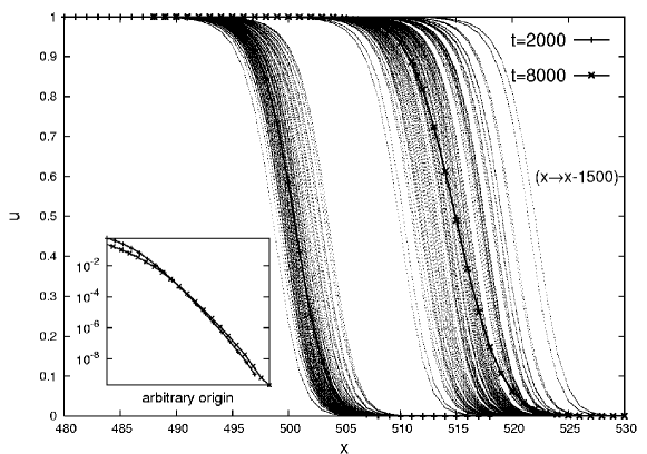
Figure 19: 1000 realizations of the evolution of the toy model between time 0 and $t_{1}=2000$ (left bunch of curves), and $t_{2}=8000$ (right bunch of curves). Insert: the average front for these two times.

We generate 1000 realizations of the stochastic evolution of our initial condition over the time intervals up to $t_{1}=2000$ and $t_{2}=8000$ respectively. The dispersion of the front positions is illustrated in Fig. 19. We see that there is roughly a factor of $\sqrt{t_{2}/t_{1}}=2$ in the dispersions between the two considered times, in agreement with Eq. (40). Each of these realizations exhibits a universal exponential shape (52) in the leading edge region, up to small fluctuations concentrated essentially in the tip. However, when taking the average, the curves for different times do not superimpose anymore, as seen in the insert of Fig. 19. Of course, this is due to the dispersion in the position of the front (40).

Now we may compute numerically the quantity

$$\frac{\sigma^{2}}{t_{f}\!-\!t_{diff}}=\left\langle\frac{\left(X_{t_{f}}\!-\!X_{t_{diff}}-\langle X_{t_{f}}\!-\!X_{t_{diff}}\rangle\right)^{2}}{t_{f}\!-\!t_{diff}}\right\rangle$$ (59)

to check the scaling form (40), (41). The result is displayed in Fig. 20. We see again a good agreement with the expectations for large values of $N$. Note that again, the $1/\ln^{3}N$ prediction overestimates the numerical calculation for smaller $N$. We have displayed on the same plot the result of the numerical calculation in the simplified model where stochastic effects are concentrated in the rightmost bin. We see again that this model gives the same result as the complete one. The discrepancies at large $N$ are statistical fluctuations, due to the fact that the plotted curve results from an average over a finite number of realizations (about 1000 here). The higher moments are more and more sensitive to such fluctuations. They should disappear when the averaging is done with more realizations.

IV.5 Consequences for QCD

So far in this section, we have discussed exclusively the toy model. Let us come back to the case of QCD. The analytical results (38)-(41) illustrated on the toy model studied in the previous section are readily taken over to QCD using Tab. 1. We list them here for completeness.

The scattering amplitude off a single partonic realization, which is not the physical observable, but is nevertheless an important intermediate quantity, reads

$$T(k,Y)\sim\frac{\ln(1/\alpha_{s}^{2})}{\pi\gamma_{0}}\sin\left(\frac{\pi\gamma_{0}\ln k^{2}/Q_{s}^{2}}{\ln(1/\alpha_{s}^{2})}\right)\left(\frac{k^{2}}{Q_{s}^{2}}\right)^{-\gamma_{0}}$$ (60)

up to fluctuations. Note that this formula is only valid in the window $1\ll\ln k^{2}/Q_{s}^{2}\ll\ln 1/\alpha_{s}^{2}$. The mean dependence of the saturation scale on rapidity reads, asymptotically for large rapidities

$$\frac{d}{dY}\langle\ln Q_{s}^{2}\rangle=\bar{\alpha}\frac{\chi(\gamma_{0})}{\gamma_{0}}-\bar{\alpha}\frac{\pi^{2}\gamma_{0}\chi^{\prime\prime}(\gamma_{0})}{2\ln^{2}(1/\alpha_{s}^{2})}\ ,$$ (61)

and its variance

$$\left\langle\left(\frac{d}{dY}\ln Q_{s}^{2}\right)^{2}\right\rangle-\left\langle\frac{d}{dY}\ln Q_{s}^{2}\right\rangle^{2}\propto\frac{\bar{\alpha}Y}{\ln^{3}(1/\alpha_{s}^{2})}\ ,$$ (62)

which, together with Eq. (60), yields the asymptotic scaling form

$$A(k,Y)=\langle T(k,Y)\rangle=A\left(\frac{\ln k^{2}-\langle\ln Q_{s}^{2}\rangle}{\sqrt{\bar{\alpha}Y/\ln^{3}(1/\alpha_{s}^{2})}}\right)\ .$$ (63)

This last formula quantifies the magnitude of the violations of geometric scaling. Note that Eq. (61) was first obtained in Ref. MS . A violation of geometric scaling was also found there, but the square root was missing in the denominator of the argument of $A$ in Eq. (63).

The formulas above are valid as long as $\bar{\alpha}Y\gg\ln^{2}(1/\alpha_{s}^{2})$, and asymptotically for $\alpha_{s}\ll 1$. For $\bar{\alpha}Y\ll\ln^{2}(1/\alpha_{s}^{2})$ instead, we have shown that fluctuations do not play a role, and the mean field discussion of Sec. III applies. This point is particularly clear in Fig. 17 and Figs. 16, 15. The kinematical regime $\bar{\alpha}Y\ll\ln^{2}(1/\alpha_{s}^{2})$ is a window where geometric scaling should be at work.

The results obtained here are exact results of QCD. They are valid for very small values of $\alpha_{s}$, where perturbation theory is justified. So the weak noise limit $N\gg 1$ or $\alpha_{s}\ll 1$ that we have considered here is the consistent expansion. Actually, as the front of the amplitude travels towards larger values of the momenta, one should take into account the running of the coupling, but this is just a (substantial!) technical complication which does not change qualitatively the picture.

Let us discuss now the validity of our results for real world QCD. As can be seen in Figs. 18 and 20, the numerical calculations get relatively close to the asymptotics at least up to a constant of order 1, for say $N>10^{4}$, which corresponds to $\alpha_{s}<10^{-2}$. Realistic attainable values of $\alpha_{s}$ in physics experiments are $\alpha_{s}>10^{-1}$. This situation would rather correspond to a strong noise limit $N\sim 1$ for which, unfortunately, no predictive theory has yet been found.

V Conclusion

In this paper, we focused on the statistical approach to high energy QCD, that we have developed and illustrated. We have shown that it provides a very simple picture for high energy scattering, relying directly on the QCD parton model. It allows a derivation from first principles of the most sophisticated analytic results that have been obtained so far for scattering amplitudes at fixed impact parameter. The simplicity of this approach is the consequence of a deep physical connection between the parton model and reaction-diffusion processes. Its main interest is to gain a simple physical understanding of the fluctuations present in the extended B-JIMWLK equations, and to enable a clear derivation of the universal asymptotics of the scattering amplitudes at high energy.

We have also solved numerically the QCD evolution equations in the context of a mean field approximation, that leads to the BK equation. We have confirmed that the BK equation admits traveling waves, and studied their formation starting with different physical initial conditions, with different definitions of the saturation scale. The numerical results have been compared to the most recent analytical predictions, and a good agreement has been found at all levels, for large enough values of the rapidity. We have also emphasized the role of the different parts of the kernel.

To go beyond the mean field approximation to high energy scattering, we have proposed and solved a toy model that captures the essential features of the full QCD evolution. The advantages of studying a toy model are numerous: in particular, it is simple enough to allow for light and flexible numerical simulations. Consequently the universal properties of the solution can be quite easily studied. We have investigated some of these properties, confirming former numerical studies on different models in the same universality class. We have investigated how the asymptotics set in. One of the important conclusions of this paper is that in the initial stages of the evolution, the mean field solution applies.

We believe that many features would still deserve to be investigated within such simplified models: for example, the effect of the running coupling would be crucial both for phenomenology and for full consistency of the approach, that relies on a small-$\alpha_{s}$ asymptotic expansion. This case would correspond to reaction-diffusion in an inhomogeneous medium, which in particular allows for a variable maximum of particles per site.

Obviously, going beyond the leading orders in rapidity and in $\alpha_{s}$ will start to be model dependent (i.e. non-universal) at some order, and the complications and specificities of QCD (color, 2-dimensional impact parameter space) will show up in the evolution equations. The same is true if one wants to give up the coarse-graining in impact parameter MSW . The solutions to the more refined equations, that is the further terms in the asymptotic expansions we have considered, will probably be difficult to obtain from the analogy with statistical mechanics that we have extensively used in this paper.

Note added: While this work was being completed, the paper Soyez appeared, that also deals with numerical solutions of QCD at high energies including fluctuations. The numerical results obtained are complementary to ours since the attitude of the author is to focus on values of $N$ realistic in the context of QCD, rather than emphasizing the connection to the analytical results obtained on equations in the universality class of the sFKPP equation.

Figures

Figure 2: Evolution of the MV initial condition using the full BK equation (21), showing ${T}(k,Y)$ for $Y=0,5\dots 50$ on a logarithmic scale and a linear scale. The $Y=0$ curve shows the initial condition.

Figure 3: Fit of the analytical formula for the reduced front to the result from the numerical calculation. Dashed line: leading order, Eq. (27). Full line: leading+next-to-leading order, Eq. (28). Points: result of the numerical integration for various values of the rapidity.

Figure 4: Propagating front, with the saturation scale for $\kappa=0.01$ marked at each value of rapidity.

Figure 5: Logarithmic derivative of the saturation scale $\frac{\partial\ln Q_{s}^{2}(Y)}{\partial Y}$ obtained from numerical simulations compared to the analytical results including two and three terms in the $Y$-expansion of Eq. (25). The saturation scale was obtained by tracking the amplitude at heights $\kappa=1.0,0.01$ and $0.0001$. The results are shown for two different rapidity ranges, and on the first plot we in addition mark the asymptotic velocity $\bar{\alpha}_{s}\chi(\gamma_{c})/\gamma_{c}\approx 0.9767$.

Figure 6: ${F}(Y)$ (Eq. (35)) for $\kappa=1.0,0.01$ and $0.0001$.

Figure 7: ${G}(Y)$ (Eq. (36)) for $\kappa=1.0,0.01$ and $0.0001$.

Figure 8: Front velocity for three different initial conditions: McLerran-Venugopalan MV , a step function, and a Gaussian.

Figure 9: Wave fronts for three different initial conditions: McLerran-Venugopalan, a step function, and a Gaussian (from the left to the right).

Figure 10: Comparison between evolution by the full BK kernel, Eq. (30), and the two-pole approximation to the kernel, Eq. (33).

Figure 11: Comparison of the logarithmic derivative of the saturation scale $\frac{\partial\ln Q_{s}^{2}(Y)}{\partial Y}$ as obtained from evolution using full BK and using the two-pole approximation of the kernel.

Figure 12: Comparison of the mean field rapidity evolutions of two different initial conditions: McLerran-Venugopalan (Eq. (34), full line), and an initial condition which behaves like $1/k$ for large $k$ (dashed line). The plot shows the logarithmic derivative of the saturation scale $\frac{\partial\ln Q_{s}^{2}(Y)}{\partial Y}$ in both cases. The straight horizontal lines are the large rapidity asymptotics (first term in Eq. (25) and Eq. (37) resp.)

Figure 13: Evolution of the shape of the front upon rapidity evolution, starting from an initial condition that behaves like $1/k$ at large $k$. The rapidity interval ranges from $Y=0$ (initial condition) to $Y=100$ (from the left to the right). The dotted lines represent $C/k$.

Figure 14: Numerical integration of the toy model defined in Eqs. (42,43) over 1000 units of time for different values of $N$.

Figure 15: Instantaneous velocity of the front as a function of time (full fluctuating line) from a numerical solution of the stochastic evolution equation (42) for $N=10^{6}$ particles per site. Large dashed curves: analytical mean field solution, asymptotics and leading correction. Short dashed curves: numerical solution of the mean field equation supplemented by a cutoff (Eq. (57)), and analytical asymptotics (Eq. (39)) (straight dashed line).

Figure 16: The same, for $N=10^{8}$ particles per site.

Figure 17: Shape of the front after an evolution of the toy model over $t_{1}=100$ (dashed steps) and $t_{2}=1000$ (full steps) steps of time. Insert: The front $u(x,t)$ compared to $e^{-\gamma_{0}x}$.

Figure 18: $v_{0}-\langle v\rangle$ from the numerical solution of the toy model, see Eq. (58) (full curve) compared to the analytical prediction (39) (full straight line). The result from the simplified toy model Eq. (50) is also displayed (dashed curve).

Figure 20: The variance of the front position divided by the time evolution interval, see Eq. (59) (full curve). Line: asymptotic prediction (40) (the overall constant being adjusted). The result from the simplified toy model Eq. (50) is also displayed (dashed curve).