MSSM Electroweak Baryogenesis and Flavour Mixing in Transport Equations

Abstract

We make use of the formalism developed in Ref. fermions , and calculate the chargino mediated baryogenesis in the Minimal Supersymmetric Standard Model. The formalism makes use of a gradient expansion of the Kadanoff-Baym equations for mixing fermions. For illustrative purposes, we first discuss the semiclassical transport equations for mixing bosons in a space-time dependent Higgs background. To calculate the baryon asymmetry, we solve a standard set of diffusion equations, according to which the chargino asymmetry is transported to the top sector, where it biases sphaleron transitions. At the end we make a qualitative and quantitative comparison of our results with the existing work. We find that the production of the baryon asymmetry of the Universe by CP-violating currents in the chargino sector is strongly constrained by measurements of electric dipole moments.

I Introduction

Electroweak baryogenesis EWBG is an effective framework for explaining the baryon asymmetry of the universe (BAU). The most appealing feature of this mechanism lies in the fact that the relevant physics will soon be explored by experiments, most notably by LHC at CERN and by the new generation of electric dipole measurements.

It has been realized that the scenario of electroweak baryogenesis depends on extensions of the Standard Model (SM), since two mandatory conditions are not met in the SM. The first reason is that CP-violation in the SM is marginal, such that the observed magnitude of baryon asymmetry cannot be explained. Secondly, the electroweak phase transition in the SM is a crossover KajantieLaineRummukainenShaposhnikov:1996 ; CsikorFodorHeitger:1998 , leading to a too weak departure from equilibrium to be viable for baryogenesis.

The Minimal Supersymmetric Standard Model (MSSM) instead has all the necessary ingredients. CP violation is enhanced by adding phases to the parameters in the soft supersymmetry breaking sector, which contribute to the chargino mass matrix. Furthermore, the additional bosonic degrees of freedom can lead to a strong first order phase transition as e.g. in the light stop scenario CarenaQuirosWagner:1996 ; Bodeker:1996pc .

These considerations indicate that the MSSM has the potential of explaining the observed BAU via electroweak baryogenesis. However, a formalism that determines the baryon asymmetry has to incorporate several features. Clearly the formalism has to reflect the quantum nature of the involved particles, for CP violation is a purely quantum effect. In addition, since the sphaleron processes are only operative in the unbroken phase, the CP-violating particle densities have to be transported away from the wall into the unbroken phase to lead to a net baryon density. A formalism that can handle both of these aspects is given by the Kadanoff-Baym equations, which are in turn derived from the out-of-equilibrium Schwinger-Dyson equations.

Early approaches that aimed to determine CP-violating densities and have not attempted to derive transport equations from first principles have been based on the dispersion relation of the quasi-particles JoyceProkopecTurok:1995 ; ClineJoyceKainulainen:1998 ; Rius:1999zc ; ClineJoyceKainulainen:2000 ; HuberSchmidt:2000+2001 deduced with the WKB method. For a recent resurrection of the method see BhattRangarajan:2004 .

In Madrid_group ; Madrid_group_imp it was suggested that an important contribution is given by mixing effects of the quasi particles in the wall rather than from the dispersion relations in the case of a nearly degenerate mass matrix. However, in the work Madrid_group ; Madrid_group_imp transport equations are not derived in a first principle approach either, but the current continuity equation is used to determine CP-violating contributions to the Green functions in a perturbative approach, which are subsequently inserted as sources into classical diffusion equations derived in Huet_Nelson . These classical diffusion equations neglect oscillations of the off-diagonal elements of the Green function that are important for a proper treatment of CP violation.

Starting from the Kadanoff-Baym equations, the authors of KPSW ; dickwerk have derived the CP-violating semiclassical force in kinetic transport equations, which appears in fermionic kinetic equation at second order in derivatives. Initially, this was done for the one fermion flavour case KPSW and then subsequently generalized to the diagonal part of the multiflavour case dickwerk .

Recently this formalism was advanced to include mixing fermions fermions . The formalism provides an accurate description of the dynamics in the thick wall regime, which applies to particles, whose de Broglie wave length is much shorter than the thickness of the phase boundary (bubble wall), formally $\partial_{x}\ll k$.

One conclusion of the work fermions is that two features of the transport equations are not captured by the procedure used in Madrid_group ; Madrid_group_imp . Firstly, the densities that are off-diagonal in the mass eigenbasis of the system will perform oscillations analogously to neutrino oscillations. This effect suppresses the transport of the CP-violating sources, especially if the mass spectrum in the chargino sector is far from degeneracy. Secondly, while Refs. Madrid_group ; Madrid_group_imp used a phenomenological prescription (Fick’s law) to introduce the CP-violating sources into the diffusion transport equations, no such prescription is required in our formalism. The sources enter the diffusion transport equations with an unambiguously defined amplitude.

A first goal of this publication is to study the simpler bosonic case, and thus to rectify the conclusions of fermions . As a second and principal goal, we consider the chargino mediated baryogenesis in the MSSM, in order to study the effects of flavour oscillations and source amplitude ambiguity on the baryon asymmetry within the framework of the reduced set of diffusion equations for charginos and quarks used in Madrid_group ; Madrid_group_imp ; BalazsCarenaMenonMorrisseyWagner:2004 ; Huet_Nelson . We also make a comparison of baryogenesis from the semiclassical force mechanism. The principal difference with respect to the previous work, is that our treatment is basis independent, while the calculations presented in Ref. ClineJoyceKainulainen:2000 ; KPSW ; dickwerk were performed in the mass eigenbasis.

This article is organized as follows. In section II we derive transport equations for mixing bosons. This is done mainly to clarify the conclusions from fermions that are present in the bosonic case, too. In the subsequent section we discuss, how the introduction of phenomenological damping terms can lead to additional unphysical CP-violating sources. The sections IV and V state the fermionic transport equations derived in fermions and the system of diffusion equations that is used to determine the baryon asymmetry. Numerical results are presented in section VI, and we conclude in section VII.

II Transport Equations for Mixing Bosons

In this section we will derive transport equations for mixing bosons from the Kadanoff-Baym equations and the resulting CP violating particle densities. This is a simpler analogon to the derivation for the fermionic case given in fermions . In the fermionic case, the spinor structure complicates the decoupling of the system of equations, but the bosonic case given here will already support the main conclusions given in fermions without the technical issues coming from the spinor structure.

II.1 Kadanoff-Baym Equations and the Approximation Scheme

Starting point are the coupled Kadanoff Baym equations dickwerk

$$e^{-i\Diamond}\{k^{2}-{{\cal M}^{2}}\}\{\Delta^{<,>}\}-e^{-i\Diamond}\{\Pi_{h}\}\{\Delta^{<,>}\}-e^{-i\Diamond}\{\Pi^{<,>}\}\{\Delta_{h}\}={\cal C},$$ (1)

$${\cal C}=\frac{1}{2}\,e^{-i\Diamond}\left(\{\Pi^{>}\}\{\Delta^{<}\}-\{\Pi^{<}\}\{\Delta^{>}\}\right),$$ (2)

where $\Delta$ denotes the Green function and $\Pi$ the self-energy of the bosons. Both quantities are $N\times N$ matrices in flavour space and depend on the average coordinate $X_{\mu}$ and the momentum variable $k_{\mu}$. The superscripts $<,>$ and the subscript $h$ denote the additional $2\times 2$ matrix structure as usual in the Kadanoff-Baym formalism

$$\Delta=\begin{pmatrix}\Delta^{++}&\Delta^{+-}\\ \Delta^{-+}&\Delta^{--}\\ \end{pmatrix},$$

$$\Delta^{<}=\Delta^{+-},\quad\Delta^{>}=\Delta^{-+},\quad\Delta^{t}=\Delta^{++},\quad\Delta^{\bar{t}}=\Delta^{--},\quad$$

$$\Delta_{h}=\Delta^{t}-\frac{1}{2}(\Delta^{<}+\Delta^{>}).$$ (3)

The diamond operator coming from the transformation into Wigner space is defined by

$$\Diamond\{a\}\{b\}\equiv\frac{1}{2}\Big{(}(\partial_{X_{\mu}}a)\partial_{k_{\mu}}b-(\partial_{k_{\mu}}a)\partial_{X_{\mu}}b\Big{)}.$$ (4)

The mass squared matrix ${{\cal M}^{2}}$ is space-time dependent and hermitian. During the electroweak phase transition, the bosonic particles relevant for baryogenesis are the squarks whose mass matrix is given by

$${\cal M}^{2}=\begin{pmatrix}m_{Q}^{2}+h_{t}^{2}H_{2}^{2}(X_{\mu})&h_{t}(A_{t}H_{2}(X_{\mu})-\mu_{c}^{*}H_{2}(X_{\mu}))\\ h_{t}(A_{t}^{*}H_{2}(X_{\mu})-\mu_{c}H_{2}(X_{\mu}))&m_{U}^{2}+h_{t}^{2}H_{2}^{2}(X_{\mu})\\ \end{pmatrix}.$$ (5)

In thermal equilibrium the Green function for a quasiparticle with mass $m$ is

$$i\Delta_{\rm eq}^{<}(k_{\mu}) = 2\pi\,\delta(k^{2}-m^{2})\textrm{ sign}(k_{0})f_{BE}(k_{0})$$

$$i\Delta_{\rm eq}^{>}(k_{\mu}) = 2\pi\,\delta(k^{2}-m^{2})\textrm{ sign}(k_{0})(1+f_{BE}(k_{0}))$$ (6)

with the Bose-Einstein distribution function

$$f_{BE}(k_{0})=\frac{1}{e^{\beta k_{0}}-1}.$$ (7)

The particle density can be deduced from the Green function using

$$j_{\nu}(X_{\mu})=2i\int_{k_{0}>0}\frac{d^{4}k}{(2\pi)^{4}}\,k_{\nu}\,\Delta^{<}(X_{\mu},k_{\mu}).$$ (8)

Since there will be already a contribution to the CP-violating particle densities in the mass term, we will in our approximation neglect interactions with other particle species. However, we will keep the collision term ${\cal C}$, since this term usually drives the system back to equilibrium and allows to fulfill the physical boundary conditions far away from the wall. We will not explicitly calculate the collision term, but finally replace it by a phenomenological damping term. Hence the Kadanoff-Baym equations simplify to

$$e^{-i\Diamond}\{k^{2}-{{\cal M}^{2}}\}\{\Delta^{<,>}\}={\cal C}.$$ (9)

A further simplification is to perform the calculation in the bubble wall frame. Our picture of the phase transition is as follows. Bubbles of the Higgs field condensate nucleate and grow at a first order electroweak transition, and as they become large, they become approximately planar. The wall frame is then defined as the frame moving with the bubble phase interface. Due to the planarity, in this frame the mass matrix depends only on the average coordinate $z:=X_{3}$. In addition as mentioned in the introduction, we are working in the thick wall regime, what makes a gradient expansion reasonable. The system expanded up to first order in gradients reads (prime denotes derivatives with respect to $z$):

$$\left(k^{2}+ik_{z}\partial_{z}+\frac{1}{4}\partial_{z}^{2}-{{\cal M}^{2}}-\frac{i}{2}{{\cal M}^{2}}^{\prime}\partial_{k_{z}}\right)\Delta^{<}={\cal C}.$$ (10)

Using the hermiticity condition $\Delta^{<\dagger}=-\Delta^{<}$ this equation can be split into its hermitian and antihermitian parts

$$\left(k^{2}+\frac{1}{4}\partial_{z}^{2}\right)\Delta^{<}-\frac{1}{2}\left\{{{\cal M}^{2}},\Delta^{<}\right\}-\frac{i}{4}\left[{{\cal M}^{2}}^{\prime},\partial_{k_{z}}\Delta^{<}\right]=0$$ (11)

$$k_{z}\partial_{z}\Delta^{<}+\frac{i}{2}\left[{{\cal M}^{2}},\Delta^{<}\right]-\frac{1}{4}\left\{{{\cal M}^{2}}^{\prime},\partial_{k_{z}}\Delta^{<}\right\}={\cal C}$$ (12)

where $\left[\cdot,\cdot\right]$ and $\left\{\cdot,\cdot\right\}$ denote commutators and anticommutators. In the following we refer to these two equations as the constraint and kinetic equation.

II.2 Lowest Order Solution

Let us first discuss equations (11–12) for a two-dimensional mass matrix that is constant in space and time. The mass matrix can be diagonalized by a unitary transformation and the equation in this basis reads (${\cal M}^{2}_{d}$ denotes the diagonalized mass matrix and $\Delta_{d}$ the corresponding Green function that is non-diagonal in general)

$$\left(k^{2}+\frac{1}{4}\partial_{z}^{2}\right)\Delta_{d}^{<}-\frac{1}{2}\left\{{\cal M}^{2}_{d},\Delta_{d}^{<}\right\}=0$$ (13)

$$k_{z}\partial_{z}\Delta_{d}^{<}+\frac{i}{2}\left[{\cal M}^{2}_{d},\Delta_{d}^{<}\right]={\cal C}_{d}\,.$$ (14)

The question is, in which sense these equations can recover the solution in thermal equilibrium (6). We expect that the Kubo-Martin-Schwinger (KMS) equilibrium condition is then satisfied, such that ${\cal C}_{d}=0$. We can use the derivative of the second equation to obtain

$$k^{2}\Delta_{d}^{<}-\frac{1}{16k_{z}^{2}}\left[{\cal M}^{2}_{d},\left[{\cal M}^{2}_{d},\Delta_{d}^{<}\right]\right]-\frac{1}{2}\left\{{\cal M}^{2}_{d},\Delta_{d}^{<}\right\}=0$$ (15)

$$k_{z}\partial_{z}\Delta_{d}^{<}+\frac{i}{2}\left[{\cal M}^{2}_{d},\Delta_{d}^{<}\right]=0\,.$$ (16)

Note that, upon the identification, $m^{\dagger}m$ ($mm^{\dagger}$) with ${\cal M}^{2}$, these equations become identical to the leading order equations obtained for the chiral fermionic distribution functions $g_{R}$ ($g_{L}$) in Ref. fermions . The constraint equation (15) is algebraic, and it determines the spectrum of the quasiparticles in the plasma. At this point it is helpful to introduce two projection operators

$$P^{T}X=\frac{1}{\Lambda^{2}}\left[{\cal M}^{2}_{d},\left[{\cal M}^{2}_{d},X\right]\right],\quad P^{D}=1-P^{T},$$ (17)

where $\Lambda:=\sqrt{\textrm{Tr}{{\cal M}^{2}}-4\textrm{ Det}{{\cal M}^{2}}}=\textrm{Tr}\,(\sigma_{3}{\cal M}^{2}_{d})$ denotes the difference of the eigenvalues of ${\cal M}^{2}_{d}$ and $\sigma_{i}$ ($i=1,2,3$) are the Pauli matrices. The properties of the projection operators

$$(P^{T})^{2}=P^{T},\quad(P^{D})^{2}=P^{D},\quad P^{T}+P^{D}=1$$ (18)

can be easily checked.

In the mass eigenbasis $P^{T}\Delta_{d}^{<}$ corresponds to the complex off-diagonal entries, while $P^{D}\Delta_{d}^{<}$ corresponds to the two real diagonal entries. If we split $\Delta^{<}_{d}$ in its transverse and diagonal parts $\Delta_{d}^{T}:=P^{T}\Delta_{d}^{<},\quad\Delta_{d}^{D}:=P^{D}\Delta_{d}^{<}$ and using the relations

$$\left\{Y^{D},X^{D}\right\}=2Y^{D}\,X^{D}, \left\{Y^{D},X^{T}\right\}=(\textrm{Tr }Y)X^{T},$$ (19)

$$P^{D}{\cal M}^{2}_{d}={\cal M}^{2}_{d}, P^{T}{\cal M}^{2}_{d}=0\,,$$ (20)

the constraint equations (15) for the diagonal and transverse parts of $\Delta_{d}^{<}$ decouple

$$\left(k^{2}-{\cal M}^{2}_{d}\right)\Delta_{d}^{D} = 0,$$ (21)

$$\left(k^{2}-\frac{\Lambda^{2}}{16k_{z}^{2}}-\frac{1}{2}\textrm{Tr }{\cal M}^{2}_{d}\right)\Delta_{d}^{T} = 0\,.$$ (22)

Both diagonal and transverse constraint equation are algebraic, and thus the solutions are given by the appropriate $\delta$-functions, which represent sharp on-shell projections. The diagonal shell is given by the standard dispersion relation, whose frequencies are, $k_{0}^{2}\equiv\omega_{i}^{2}=\vec{k}^{2}+m_{i}^{2}$, where $m_{i}^{2}$ are the eigenvalues of ${{\cal M}^{2}}$. The transverse parts fulfill a different on-shell condition, which can be easily obtained from (22). Note that these on-shell conditions are the same as the ones found in fermions by solving the leading order constraint equations for fermions.

The kinetic equation (16) reveals another difference between diagonal and transverse parts. The kinetic equations read

$$k_{z}\partial_{z}\Delta_{d}^{D} = 0,$$ (23)

$$k_{z}\partial_{z}\Delta_{d}^{T}+\frac{i}{2}\left[{\cal M}^{2}_{d},\Delta_{d}^{T}\right] = 0\,.$$ (24)

The diagonal parts are constant in space and time, while the transverse parts rotate in flavour space with the frequency $\sim{\Lambda}/{k_{z}}$.

In the equilibrium solution (6) the transverse entries vanish everywhere, but it is clear that this oscillation dominates the dynamics of the transverse parts as soon as they are sourced by higher order contributions in the gradient expansion.

Alternatively, oscillations can be induced by the initial conditions. This is, for example, the case in neutrino oscillations. Neutrinos are namely created as flavor eigenstates, and hence, from the point of view of the mass eigenbasis, a mixture of diagonal and transverse states. Since in most environments the damping of neutrinos is very small, neutrino oscillations persist for a long time.

II.3 First order solution and CP violation

Let us consider again the Kadanoff-Baym equations (11–12) to first order in gradients. In the last section we saw that in lowest order the spectrum can be separated into the diagonal and transverse contributions. One can show that in the first order system (11–12) however, the different quasiparticles start to mix and the spectral functions acquire a finite width. This is reflected in the fact that, at first order in gradients, the constraint equation is not any more algebraic.

Fortunately we do not need any information about the spectrum to solve the kinetic equation (12), since it does not explicitly contain any $k_{0}$ dependence. When transformed into the mass eigenbasis, the kinetic equation reads

$$k_{z}\partial_{z}\Delta_{d}^{<}+k_{z}\left[\Sigma,\Delta_{d}^{<}\right]+\frac{i}{2}\left[{\cal M}^{2}_{d},\Delta_{d}^{<}\right]-\frac{1}{4}\left\{{{\cal M}^{2}_{d}}^{\prime}+\left[\Sigma,{\cal M}^{2}_{d}\right],\partial_{k_{z}}\Delta_{d}^{<}\right\}={\cal C}_{d}$$ (25)

with

$$\Sigma=U^{\dagger}U^{\prime}$$ (26)

and the matrix $U(z)$ diagonalizes ${{\cal M}^{2}}$, ${\cal M}^{2}_{d}=U^{\dagger}{{\cal M}^{2}}U$.

The next step is to determine the CP violating contributions to the particle densities. By definition the CP conjugation acts as

$$\Delta_{d}^{{\cal CP}}(X,k)\,\equiv\,{\cal CP}\,\,\Delta_{d}(X,k)\,\,{\cal CP}\,=\,\Delta_{d}^{*}(\bar{X},-\bar{k}),$$ (27)

$$\quad\bar{X}^{\mu}=(X_{0},-X_{i}),\quad\bar{k}^{\mu}=(k_{0},-k_{i})\,.$$ (28)

This transformation is in our equation (25) equivalent to

$$U\rightarrow U^{*},\quad\Sigma\rightarrow\Sigma^{*}\,.$$ (29)

Now suppose that as in the chargino case our particles do not directly couple to the sphaleron process. Then the CP-violating particle density has to be communicated to the other species via interactions. Therefore we are rather interested in the CP violating densities in the diagonal matrix elements of the Green function in the interaction eigenbasis. These are given by

$$\textrm{Tr }[\Delta^{<}-{\cal CP}\,\Delta^{<}{\cal CP}] = \textrm{Tr }\big{[}U\Delta_{d}^{<}U^{\dagger}-U^{*}\,\Delta^{<{\cal CP}}_{d}U^{\dagger*}\big{]}$$ (30)

$$= \textrm{Tr }\big{[}U(\Delta_{d}^{<}-\Delta^{<{\cal CP}*}_{d})U^{\dagger}\big{]}$$

and

$$\textrm{Tr }\big{[}\sigma_{3}\Delta^{<}-\sigma_{3}{\cal CP}\,\Delta^{<}{\cal CP}\big{]} = \textrm{Tr }\big{[}\sigma_{3}U\Delta_{d}^{<}U^{\dagger}-\sigma_{3}U^{*}\,\Delta^{<{\cal CP}}_{d}U^{\dagger*}\big{]}$$ (31)

$$= \textrm{Tr }\big{[}\sigma_{3}U(\Delta_{d}^{<}-\Delta^{<{\cal CP}*}_{d})U^{\dagger}\big{]},$$

where the latter equality in both cases follows from the fact that $\Delta_{d}^{<{\cal CP}}$ is hermitian. Henceforth we consider in the mass eigenbasis the equation for $\Delta^{<{\cal Q}}:=\Delta^{<{\cal CP}*}$. This Q-conjugation coincides with CP-conjugation on the diagonal, but it is in addition basis independent, since it commutes with the diagonalization matrix. This fact was already used in fermions to identify CP-violating quantities for mixing fermions before the Green function was transformed to the interaction eigenbasis.

The equation for $\Delta^{<{\cal Q}}$ is given by (notice that $\Sigma$ is antihermitian)

$$k_{z}\partial_{z}\Delta_{d}^{<{\cal Q}}+k_{z}\left[\Sigma,\Delta_{d}^{<{\cal Q}}\right]-\frac{i}{2}\left[{\cal M}^{2}_{d},\Delta_{d}^{<{\cal Q}}\right]-\frac{1}{4}\Big{\{}{{\cal M}^{2}_{d}}^{\prime}+\left[\Sigma,{\cal M}^{2}_{d}\right],\partial_{k_{z}}\Delta_{d}^{<{\cal Q}}\Big{\}}={\cal C}_{d}\,.$$ (32)

The only change with respect to the original equation of $\Delta_{d}^{<}$ is a sign-change in the oscillation term $\big{[}{\cal M}^{2}_{d},\Delta_{d}^{<Q}\big{]}$. If we include higher order terms in the gradient expansion additional Q breaking terms will appear. Since in leading order CP violation is based on the oscillation effect, one has to solve only the equation of the transverse parts and its Q conjugate. Collecting terms, that are at most first order in gradients (deviations from equilibrium $\delta\Delta_{d}=\Delta_{d}-\Delta_{\rm eq}$, ${{\cal M}^{2}_{d}}^{\prime}$ and $\Sigma$ are counted as of order one in the gradient expansion) we get for the transverse deviations,

$$k_{z}\partial_{z}\delta\Delta_{d}^{T}+\;\frac{i}{2}\left[{\cal M}^{2}_{d},\delta\Delta_{d}^{T}\right]\;-{\cal C}_{d} = {\cal S}_{d}$$

$$k_{z}\partial_{z}\delta\Delta_{d}^{T{\cal Q}}-\frac{i}{2}\left[{\cal M}^{2}_{d},\delta\Delta_{d}^{T{\cal Q}}\right]-{\cal C}_{d} = {\cal S}_{d}\,,$$ (33)

with the source term

$${\cal S}_{d}=-k_{z}\left[\Sigma,\Delta_{\rm eq}^{<}\right]^{T}+\frac{1}{4}\left\{{{\cal M}^{2}_{d}}^{\prime}+\left[\Sigma,{\cal M}^{2}_{d}\right],\partial_{k_{z}}\Delta_{\rm eq}^{<}\right\}^{T}\,.$$ (34)

This can be solved numerically using an Ansatz for a flow solution as described in Ref. fermions .

Since $\Delta_{d}^{<CP}$ and $\Delta_{d}^{<Q}$ differ only by transposition, this calculation in addition shows that the diagonal entries in the mass eigenbasis will be CP even up to first order in gradients.

III The Damping Term

If we solve equations (33) without the collision term, we will have problems to ensure that our solution will be close to thermal equilibrium on both sides at a large distance from the wall. This problem can be solved by introducing a damping term, that corresponds to statistical effects due to the interaction of the particles with the heat bath. In the rest frame of the plasma, the damping should take place in the positive time like direction as e.g. in the equation

$$k\cdot\partial_{X}\Delta+k_{0}\Gamma\Delta={\cal S}$$ (35)

In the wall frame this leads to ${\cal C}_{d}=\gamma_{v_{w}}(k_{0}-v_{w}k_{z})\,\Gamma\,\Delta$ with the wall velocity $v_{w}$. For $\Gamma$ a reasonable choice is $\Gamma=\alpha T_{c}$, where $\alpha$ denotes the coupling strength of the dominant interaction of the species and $T_{c}$ is the temperature of the plasma during the phase transition.

However, by introducing a term that breaks time reversal invariance, we run the risk of breaking CP explicitly by introducing new artificial CP-violating sources. We illustrate this by the following simple example. Assume that a quantity $W$, which denotes a CP-violating deviation from equilibrium, fulfills the equation

$$\partial_{z}\,W=\exp(-z^{2})\,n_{BE}(\sqrt{k_{z}^{2}+m^{2}})\equiv{\cal S}(z,k_{z})$$ (36)

and we are interested in $\int dk_{z}\,W(z,k_{z})$.

To solve this equation, we can use the Green function method with the boundary condition, such that $W$ vanishes in the unbroken phase ($z\to-\infty$), where the wall has not yet influenced the plasma. Then

$$W(z,k_{z})=\int dz^{\prime}\,\,g(z,z^{\prime})\,\,{\cal S}(z^{\prime},k_{z})\,,$$ (37)

with the Green function

$$g(z,z^{\prime})=\theta(z-z^{\prime})$$ (38)

and $\int dk\,W(z,k_{z})$ can be determined.

Since the solution does not vanish in the broken phase ($z\to+\infty$), we introduce a phenomenological damping term that breaks time invariance and our choice could be in analogy to the considerations above

$$\partial_{z}W+\frac{k_{0}}{k_{z}}\Gamma\,\,W={\cal S}(z,k_{z})$$ (39)

The corresponding Green function is

$$g(z,y)=\left\{\begin{matrix}k_{0}/k_{z}>0:&\exp\Big{(}-({k_{0}}/{k_{z}})\Gamma(z-z^{\prime})\Big{)}\,\theta(z-z^{\prime})\\ k_{0}/k_{z}<0:&-\exp\Big{(}({k_{0}}/{k_{z}})\Gamma(z-z^{\prime})\Big{)}\,\theta(z^{\prime}-z)\end{matrix}\right.$$ (40)

and yields the desired result. On the other hand, if the source is odd in $k_{z}$, the picture changes. The equation (37) yields a solution, that is odd in $k_{z}$ and $\int dk_{z}\,W(z,k_{z})$ vanishes, while the solution of (39) gives a non-vanishing result even after integration over $k_{z}$.

The same effect can be seen in the kinetic equation (33). Without the damping term, the result will be odd in $k_{z}$, such that only the three component of the particle current

$$j_{\nu}(X_{\mu})=2i\int_{k_{0}>0}\frac{d^{4}k}{(2\pi)^{4}}\,k_{\nu}\,\Delta(X_{\mu},k_{\mu}).$$ (41)

is sourced. This is expected, since if this current is Lorentz boosted into the rest frame of the plasma, the CP-violating particle density $j_{0}^{plasma-frame}=\gamma_{v_{w}}\,v_{w}\,j_{3}^{wall-frame}$ vanishes in the static wall limit, $v_{w}=0$.

After the damping term is introduced, $j_{0}^{plasma-frame}$ is sourced even in the case of a static wall profile, which is clearly an unphysical result for a CP-violating quantity. Notice that this source persists even in the limit $\Gamma_{h}\to 0$. In the following we keep only the source terms, which are not induced by the damping term.

IV Transport Equations for Mixing Charginos

In this section we recall the fermionic transport equations derived in fermions . Due to the additional spinor structure of the Green function, we have to solve two equations for the left-handed and right-handed densities separately. In addition, the Green functions have a spin quantum number $s$. As in the bosonic case, only the transverse parts oscillate and contribute to the CP-violating (or better Q-violating) densities. In the mass eigenbasis the equations for $\delta g_{Rd}^{Ts}$ and $\delta g_{Ld}^{Ts}$ read (see Eq. (78) in Ref. fermions )

$$k_{z}\partial_{z}\delta g_{Rd}^{Ts}+\frac{i}{2}\left[m^{2}_{d},\delta g_{Rd}^{Ts}\right]+k_{0}\Gamma_{h}\delta g_{Rd}^{Ts} = {\cal S}_{R}^{s}$$ (42)

$$k_{z}\partial_{z}\delta g_{Ld}^{Ts}+\frac{i}{2}\left[m_{d}^{2},\delta g_{Ld}^{Ts}\right]+k_{0}\Gamma_{h}\delta g_{Ld}^{Ts} = {\cal S}_{L}^{s}\,,$$ (43)

with the spin-dependent part of the sources

$${\cal S}_{R}^{s} = -s\frac{k_{z}^{2}}{\tilde{k}_{0}}\left[VV^{\dagger\prime},g_{0,\rm eq}\right]-\frac{s}{4\tilde{k}_{0}}\left[V(m^{\dagger\prime}m-m^{\dagger}m^{\prime})V^{\dagger},g_{0,\rm eq}\right]+\frac{sk_{z}}{4\tilde{k}_{0}}\left\{V(m^{\dagger}m)^{\prime}V^{\dagger},g_{0,\rm eq}\right\}^{T}$$

$${\cal S}_{L}^{s} = s\frac{k_{z}^{2}}{\tilde{k}_{0}}\left[UU^{\dagger\prime},g_{0,\rm eq}\right]+\frac{s}{4\tilde{k}_{0}}\left[U(m^{\prime}m^{\dagger}-mm^{\dagger\prime})U^{\dagger},g_{0,\rm eq}\right]-\frac{sk_{z}}{4\tilde{k}_{0}}\left\{U(mm^{\dagger})^{\prime}U^{\dagger},g_{0,\rm eq}\right\}^{T}\!\!.\quad$$ (44)

The function $g_{0,\rm eq}$ denotes the $\gamma_{0}$ coefficient of the Green function in thermal equilibrium and mass eigenbasis

$$g_{0,\rm eq}=2\pi|k_{0}|\delta(k^{2}-m_{d}^{2})f_{FD},\quad f_{FD}=\frac{1}{e^{\beta k_{0}}+1}.$$ (45)

The chargino mass matrix $m$ is given by

$$m=\left(\begin{array}[]{cc}M_{2}&gH_{2}\cr gH_{1}&\mu_{c}\cr\end{array}\right)$$ (46)

and diagonalized by the biunitary transformation

$$m_{d}=UmV^{\dagger}\,,$$ (47)

where $\mu_{c}$ and $M_{2}$ are the soft supersymmetry breaking parameters.

To compare the result from these equations with the work Madrid_group ; Madrid_group_imp it is helpful to examine the contributions of the different sources in the local approximation, $\Gamma_{h}\to\infty$, in which diffusion transport is neglected. In this case, the resulting CP-violating vector and axial vector particle currents behave as

$$\hskip-56.9055pt{\rm Tr}\big{(}\sigma^{3}j_{5\,\mu}\big{)}={\cal S}^{a}_{\mu},\quad{\rm Tr}\big{(}\sigma^{3}j_{\mu}\big{)}={\cal S}^{b}_{\mu}+{\cal S}^{c}_{\mu}$$

$${\cal S}^{a}_{\mu} = 2T_{c}^{-4}\Im(M_{2}\mu_{c})(|M_{2}|^{2}-|\mu_{c}|^{2})\partial_{\mu}\big{(}u_{1}u_{2}\big{)}\eta_{(0)}^{3}$$

$${\cal S}^{b}_{\mu} = 2T_{c}^{-4}\Im(M_{2}\mu_{c})(u_{1}^{2}-u_{2}^{2})\partial_{\mu}(u_{1}u_{2})\eta_{(0)}^{3}$$

$${\cal S}^{c}_{\mu} = -2T_{c}^{-2}\Im(M_{2}\mu_{c})\big{(}u_{2}\partial_{\mu}u_{1}-u_{1}\partial_{\mu}u_{2}\big{)}\big{(}\eta_{(0)}^{0}+4\eta_{(2)}^{3}\big{)}\,,$$ (48)

where $u_{1,2}=g|H_{1,2}|$, and $\eta_{(0)}^{0}$, $\eta_{(0)}^{3}$ and $\eta_{(2)}^{3}$ are integrals derived in fermions ,

$$\eta_{(n)1,2} = T_{c}^{2-n}\int_{k_{0}>0}\frac{d^{4}k}{(2\pi)^{3}}\frac{k_{0}}{\tilde{k}_{0}}k_{z}^{n}\frac{n(k^{\mu},m^{2}_{1,2})}{k_{0}^{2}\Gamma_{h}^{2}+(\Lambda/2)^{2}}\delta(k^{2}-m_{1,2}^{2})$$

$$\eta_{(n)}^{0} = \frac{1}{2}\big{(}\eta_{(n)1}+\eta_{(n)2}\big{)}\,,\qquad\eta_{(n)}^{3}=\frac{T_{c}^{2}}{2\Lambda}\big{(}\eta_{(n)1}-\eta_{(n)2}\big{)}\,,$$ (49)

and $n=n(k^{\mu},m^{2}_{1,2})$ denotes the distribution function. The contributions ${\cal S}_{a}$ and ${\cal S}_{b}$ result from the first term in the sources (44), while the term ${\cal S}_{c}$ results from the second and third terms in the sources (44).

Comparing with Eq. (3.13) of Madrid_group_imp , we see that in local approximation our sources agree in the characteristics of the $z$-dependence, but show different structure in momentum space.

To facilitate a comparison with the work on semiclassical force baryogenesis of Cline, Joyce and Kainulainen ClineJoyceKainulainen:2000 , we quote the dominating local source at the second order in gradients in the plasma frame fermions ; dickwerk ,

$$\textrm{Tr}\left(\mathbbm{1}\,j^{(2)}_{5,0}\right)\equiv{\cal S}^{d}_{0}=2\,v_{w}\,T_{c}^{-4}\Im(M_{2}\mu_{c})\big{(}u_{2}\partial^{2}_{z}u_{1}+u_{1}\partial^{2}_{z}u_{2}\big{)}\zeta_{(0)}^{3}\,,$$ (50)

where $\zeta_{(0)}^{3}=\eta_{(0)}^{3}|_{\Lambda\rightarrow 0}$. This source corresponds to the CP-violating shift in the dispersion relation and dominates if the mass spectrum in the chargino sector is far from degeneracy ($\Lambda\to\infty$) and in the limit of a small damping. It contributes in contrast to the first order terms to the trace of the chargino current.

V Diffusion Equations

Using our formalism, we can deduce the CP-violating particle densities in the chargino sector. To evaluate the baryon asymmetry in the broken phase, we need to compute the density of left-handed quarks and leptons $n_{L}$ in front of the wall. These densities couple to the weak sphaleron and produce a net baryon number.

To determine how the CP-violating currents are transported from the charginos to the left-handed quarks and leptons we use a system of coupled diffusion equations as derived in Huet_Nelson , and later adapted in Carena:1997gx ; Madrid_group and ClineJoyceKainulainen:2000 . The diffusion equations are

$$v_{w}\,n_{Q}^{\prime} = D_{q}\,n^{\prime\prime}_{Q}-\Gamma_{Y}\left[\frac{n_{Q}}{k_{Q}}-\frac{n_{T}}{k_{T}}-\frac{n_{H}+n_{h}}{k_{H}}\right]-\Gamma_{m}\left[\frac{n_{Q}}{k_{Q}}-\frac{n_{T}}{k_{T}}\right]$$ (51)

$$-6\,\Gamma_{ss}\left[2\,\frac{n_{Q}}{k_{Q}}-\frac{n_{T}}{k_{T}}+9\,\frac{n_{Q}+n_{T}}{k_{B}}\right]$$

$$v_{w}\,n_{T}^{\prime} = D_{q}\,n^{\prime\prime}_{T}+\Gamma_{Y}\left[\frac{n_{Q}}{k_{Q}}-\frac{n_{T}}{k_{T}}-\frac{n_{H}+n_{h}}{k_{H}}\right]+\Gamma_{m}\left[\frac{n_{Q}}{k_{Q}}-\frac{n_{T}}{k_{T}}\right]$$ (52)

$$+3\,\Gamma_{ss}\left[2\,\frac{n_{Q}}{k_{Q}}-\frac{n_{T}}{k_{T}}+9\,\frac{n_{Q}+n_{T}}{k_{B}}\right]$$

$$v_{w}\,n_{H}^{\prime} = D_{h}\,n^{\prime\prime}_{H}+\Gamma_{Y}\left[\frac{n_{Q}}{k_{Q}}-\frac{n_{T}}{k_{T}}-\frac{n_{H}+n_{h}}{k_{H}}\right]-\Gamma_{h}\frac{n_{H}}{k_{H}}$$ (53)

$$v_{w}\,n_{h}^{\prime} = D_{h}\,n^{\prime\prime}_{h}+\Gamma_{Y}\left[\frac{n_{Q}}{k_{Q}}-\frac{n_{T}}{k_{T}}-\frac{n_{H}+n_{h}}{k_{H}}\right]-(\Gamma_{h}+4\Gamma_{\mu})\frac{n_{h}}{k_{H}}\,,$$ (54)

where $n_{T}$ denotes the density of the left-handed top and stop particles, $n_{Q}$ the remaining left-handed quarks and squarks and $n_{H}$ and $n_{h}$ the sum and difference of the two Higgsino densities $n_{H_{1}}$ and $n_{H_{2}}$. The quantities $k_{i}$ are statistical factors defined by $n_{i}=k_{i}\,\mu_{i}\frac{T_{c}^{2}}{6}$ ($\mu_{i}$ denotes the chemical potential of species $i$). For light, weakly interacting particles $k_{i}\approx 2$ (bosons) or $k_{i}\approx 1$ (fermions), while for particles much heavier than $T_{c}$, $k_{i}$ is exponentially small. We use the values

$$k_{Q}\approx 6,\quad k_{T}\approx 9,\quad k_{B}\approx 3,\quad k_{H}\approx 12$$ (55)

corresponding to the light stop scenario Huet_Nelson and the diffusion constants are JoyceProkopecTurok:1994-I

$$D_{q}\sim 6/T_{c},\quad D_{h}\sim 110/T_{c}.$$ (56)

For the particle number changing rates we take JoyceProkopecTurok:1994-I ; JoyceProkopecTurok:1995 ; Huet_Nelson ,

$$\Gamma_{y}\approx\frac{1}{10}T_{c},\quad\Gamma_{m}\approx\frac{1}{10}T_{c},\quad\Gamma_{h}\approx\frac{1}{20}T_{c},\quad\Gamma_{\mu}\approx\frac{1}{10}T_{c}$$ (57)

and for the sphaleron rates sphaleron

$$\Gamma_{ss}\approx 1.5\times 10^{-2}\,T_{c},\quad\Gamma_{ws}\approx 6.0\times 10^{-6}\,T_{c}.$$ (58)

The diffusion equations (51–54) are derived under the assumptions ClineJoyceKainulainen:2000 that (a) the supergauge interactions, which are of the weak strength, are in equilibrium; (b) the chargino asymmetry gets transported to the quark sector via the strong top Yukawa interactions, while the wino asymmetry does not contribute; (c) the gaugino helicity-flip interactions are in equilibrium, implying that the chemical potentials for particles and their supersymmetric partners are equal. These approximations imply that the main channel for baryon production is the conversion of the chargino asymmetry into the top sector, which then bias electroweak sphalerons. The accuracy of these approximations will be addressed elsewhere.

The solution of Eqs. (51–54) is performed in several steps. First we use the transport equations in the chargino sector as described in fermions to determine $n_{H}$ and $n_{h}$. The result is used as an input in the equations (51) and (52). From these equations the left-handed particle density $n_{L}=5\,n_{Q}+4\,n_{T}$ can be determined and used as a source for the weak sphaleron process as described in Madrid_group (see also Ref. ClineKainulainen:2000 ). The net baryon density is given by

$$n_{B}=-\frac{3\,\Gamma_{ws}}{v_{w}}\int_{-\infty}^{0}dz\,\,n_{L}(z)\exp\left(z\frac{15\Gamma_{ws}}{4\,v_{w}}\right)$$ (59)

and finally the baryon-to-entropy ratio is determined via

$$\eta=\frac{n_{B}}{s},\quad s=\frac{2\pi^{2}}{45}g_{\rm eff}T_{c}^{3}\approx 51.1\,\,T_{c}^{3}.$$ (60)

To check, whether our solution of the diffusion equation is consistent, we used the densities $n_{Q}$ and $n_{T}$ as input for the equations (53) and (54). The resulting deviations in the Higgsino densities never exceed $5\%$ of the original densities. This is due to the fact that the Higgsino diffusion constant $D_{h}$ is rather large and that the oscillation partially suppresses an efficient transport of the quarks and squarks. In this light the equations of the Higgsinos decouple, since the oscillation provides the shortest time-scale.

Note that in the work Giudice:1993bb a suppression was found for the parameters of the Standard Model ($k_{T}\approx 3$ in Eq. (55)). As explained, for the mixing sources we consider here, the oscillation effectively decouples the dynamics of the charginos from the quarks/squarks. This allows us to neglect the backreactions from the quarks/squarks and leads to the absence of the suppression for $k_{T}\approx 3$. If the oscillation is not the shortest time-scale, i.e. for $|\mu_{c}-M_{2}|<5$ GeV, the backreactions become large and our approach does not reproduce the suppression of Giudice:1993bb and would indeed over-estimate the result. In the following we will employ the parameters of Eq. (55) where this suppression mechanism is already ineffective.

VI Numerical Results

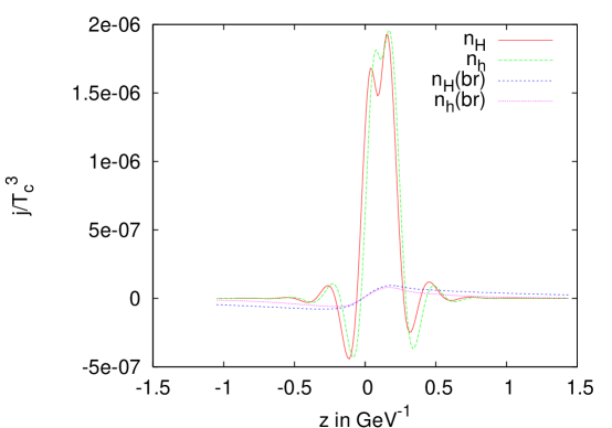
Figure 1: The original Higgsino densities and the corresponding back-reactions. The parameters of the plot are $\mu_{c}=200$ GeV, $M_{2}=180$ GeV, $m_{A}=200$ GeV

In this section we will present numerical results of the transport and diffusion equations. The Higgs vevs and the $\beta$ angle are parametrized by

$$H_{1}(z)=H(z)\sin(\beta(z)),\quad H_{2}(z)=H(z)\cos(\beta(z))$$ (61)

and

$$H(z)=\frac{1}{2}v(T)\left(1-\tanh\left(\alpha\left(1-\frac{2z}{L_{w}}\right)\right)\right),$$ (62)

$$\beta(z)=\beta_{\infty}-\frac{1}{2}\Delta\beta\left(1+\tanh\left(\alpha\left(1-\frac{2z}{L_{w}}\right)\right)\right).$$ (63)

The parameters used are

$$T_{c}=110~{}{\rm GeV},\quad v(T)=175~{}{\rm GeV},\quad\alpha=\frac{3}{2},\quad\tan(\beta_{\infty})=10,\quad L_{w}=20/T_{c}$$ (64)

and the complex phase is chosen maximally

$$\Im(M_{2}\mu_{c})=|M_{2}\mu_{c}|\,.$$ (65)

We have checked, with the help of a program developed by the authors of Refs. Madrid_group ; Carena:1997ki , that the values for $v(T)$ compatible with present Higgs bounds typically lie in the range 165-185 GeV. The exact value depends on parameters of the Higgs and squark sectors which affect our results only through this expectation value. We therefore have fixed the value of $v(T)$ to its zero temperature result. The uncertainty arising from our choice is below ten percent.

The values of $\Delta\beta$ are deduced from Moreno_Seco_PT for the different values of $m_{A}$. The wall velocity is taken to be $v_{w}=0.05$ and the transport equations are evaluated using the fluid Ansatz for the first six momenta. The parameters of the diffusion equations are given in the last section.

The plot Fig. 1 supports the claim that, within our approximations and for our choice of parameters, the back-reaction of left-handed quarks and squarks, $n_{Q}$, $n_{T}$, on the charginos can be neglected. The amplitude of the Higgsino densities coming from the back-reaction is always smaller than $3\%$ and never leads to corrections of the baryon-to-entropy ratio larger than $5\%$.

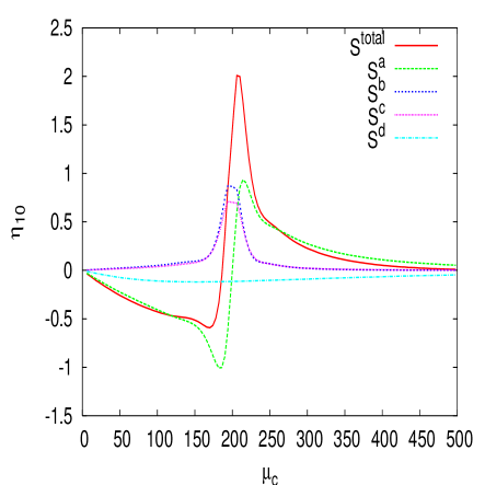
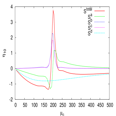
Figure 2: This plot shows the first and second order sources as a function of $\mu_{c}$ with $M_{2}=200$ GeV. The plot on the left are the sources with the damping, $\Gamma=\alpha_{w}T_{c}$, while on the right plot, $\Gamma=0.25\alpha_{w}T_{c}$.

In Fig. 2 we plot the first order sources ${\cal S}_{\mu}^{a}$, ${\cal S}_{\mu}^{b}$, ${\cal S}_{\mu}^{c}$ and the second order source (semiclassical force) ${\cal S}^{d}$, as defined in Eqs. (48–50). The first order sources are roughly of the same magnitude, and they peak when $|\mu_{c}|\simeq|M_{2}|$, where they also switch the sign. The second order source varies slowly with $|\mu_{c}|$ and tends to dominates when the difference $|\mu_{c}|-|M_{2}|$ becomes large. Note that when the damping is small, the first order sources become more peaked around $|\mu_{c}|=|M_{2}|$, but the amplitude of the baryon asymmetry does not significantly change. On the other hand, the second order source is about an order of magnitude larger in the right plot, implying that in the limit of a small damping the second order source (semiclassical force) may result in a viable baryogenesis. Since our damping term is phenomenological and flavor blind, it would be premature to conclude that the second order source cannot lead to a viable baryogenesis, until a more quantitative analysis of the damping term is performed.

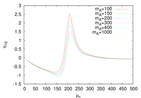
Figure 3: This plot shows $\eta_{10}=10^{10}\eta$ as a function of $\mu_{c}$ with $M_{2}=200$ GeV and for several values of $m_{A}$ in GeV.

The parameters chosen in Figs. 3 and 4 are similar to the ones chosen in Madrid_group_imp , in order to facilitate comparison. In plot Fig. 3 the parameters $m_{A}$ and $M_{2}$ are fixed while $\mu_{c}$ is varied. The maximum is not exactly at $\mu_{c}=M_{2}$ as in Madrid_group_imp , but rather close to $\mu_{c}\approx M_{2}+20$ GeV. The reason for this difference is that in our case all sources (48) are of similar order, while in Madrid_group_imp , the baryon asymmetry is completely dominated by a source term of form ${\cal S}_{\mu}^{c}$ in (48) that is proportional to $\Delta\beta$ in the parametrization (63) and hence suppressed for large values of $m_{A}$ as shown in Moreno_Seco_PT . Another difference is that our plot shows the suppression for $\mu_{c}\gg M_{2}$ what is expected since in this case the quasi-particles have highly separated on-shell conditions and mixing should be suppressed. We would like to emphasize that the peak around $\mu_{c}\approx M_{2}+20$ GeV is due to this suppression and not due to a resonance in the sources as it was in the publications Riotto:1998zb ; Madrid_group ; Madrid_group_imp and more recently in Lee:2004we . In the present work, the sources show a resonance but the CP-violating densities do not since they are generated by the oscillations (see Eq. (33) ) and contain near the degeneracy an additional proportionality to the mass splitting $\Lambda$. In Fig. 4 the baryon asymmetry is plotted near the maximal value $\mu_{c}\approx M_{2}+20$ GeV. The maximum is reached near $\mu_{c}\approx 80$ GeV in contrast to Madrid_group_imp where the maximum was $\mu_{c}\approx 250$ GeV.

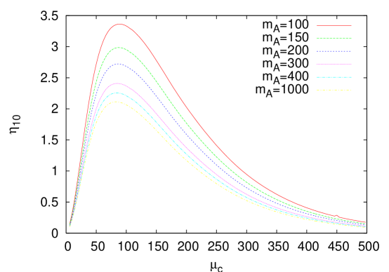
Figure 4: This plot shows $\eta_{10}=10^{10}\eta$ as a function of $\mu_{c}$, $M_{2}=\mu_{c}-20$ GeV and for several values of $m_{A}$ (in GeV) .

Finally in Fig. 5 two contour plots are shown with regions in the $(M_{2},\mu_{c})$ parameter space for the baryon asymmetry expressed in terms of $\eta_{10}\equiv 10^{10}\times\eta$. In these units the observed value is close to unity, $\eta_{10,\rm obs}=0.8-0.9$. If $\eta_{10}>\eta_{10,\rm obs}$, the observed value can be attained simply by adjusting the complex phase, which is in our calculation chosen to be maximal. The two plots correspond to the choices $m_{A}=200$ GeV and $m_{A}=400$ GeV.

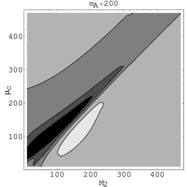
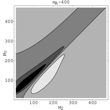
Figure 5: The baryon-to-entropy ratio $\eta_{10}=10^{10}\times\eta$ in the $(M_{2},\mu_{c})$ parameter space from (0 GeV,0 GeV) to (500 GeV,500 GeV). For the left plot the value $m_{A}=200$ GeV is used, for the right plot $m_{A}=400$ GeV. The black region denotes $\eta_{10}>1$, where baryogenesis is viable. The other four regions are bordered by the values of $\eta_{10}$, $\{-0.5,0,0.5,1\}$, beginning with the lightest color.

In the following we will comment on differences between the formalism used in this paper and the work Madrid_group_imp that lead to the discrepancy in the numerical results . As already mentioned in a previous section the authors in Madrid_group_imp work in the flavour basis and write classical Boltzmann equations using CP-violating sources whereas in this work the sources appear genuinely in a basis independent set of quantum transport equations. In this work the damping $\Gamma_{h}$ is primarily introduced to obtain consistent boundary conditions and it corresponds to the helicity flip rate $\Gamma_{h}$ in the diffusion equations of Madrid_group . We have excluded $\Gamma_{h}$ dependent terms that violate CP and the limit $\Gamma_{h}\rightarrow 0$ is straightforward.

In addition to the damping $\Gamma_{h}$ a Breit-Wigner width $\Gamma_{\tilde{t}}$ was introduced in the chargino spectrum in Madrid_group . We have checked in the simpler bosonic case that, for $\Gamma_{\tilde{t}}\to 0$, the present sources and those in Madrid_group are related in a simple way. A detailed discussion is presented in the Appendix. Of course, the ambiguity related to the magnitude of the source in the chargino diffusion equations remains in the formalism used in Refs. Madrid_group ; Madrid_group_imp , where a phenomenological thermalization time $\tau$ or the classical Fick’s law had to be used to incorporate the sources into the diffusion equations. In our formalism the magnitude of the source is completely specified.

Furthermore, we have checked that the effect of the Breit-Wigner broadening on our sources is small. This effect can be modeled by replacing the $\delta$-function in (45) by the corresponding Breit-Wigner form. To account for the finite $\Gamma_{\tilde{t}}$ in the transport and not just in the sources is on the same level as a treatment of the collision terms in Refs. Kainulainen:2002sw ; dickwerk ; Lee:2004we and it is outside the scope of this paper. In principle, the collision term could as well yield additional CP-violating sources, but a one-loop calculation dickwerk in a model theory of chiral fermions Yukawa-coupled to scalars, indicates that the collisional sources are phase space suppressed with respect to our tree level sources.

VII Conclusions and Discussion

In this work we obtained the baryon asymmetry of the universe during the electroweak phase transition in the MSSM using semiclassical transport equations derived in a first principle approach from the Kadanoff-Baym (KB) equations in Ref. fermions . When the KB equations are expanded in gradients in the general case of mixing fermions, the CP-violating deviations from equilibrium can be sourced by a space-time dependent Higgs background both at first and second order in gradients. The first order effects, which occur only in the presence of fermion mixing, have been consistently determined including oscillations that are crucial for the dynamics of the CP-violating densities. The second order effects are dominated by the semiclassical force JoyceProkopecTurok:1995 ; dickwerk ; ClineJoyceKainulainen:2000 , which is the leading order source for single fermions coupled to a space-time dependent background. Unlike in some alternative approaches pursued in the literature, a nice feature of the present approach is that sources and transport are treated within one formalism, which allows for an unambiguous fixing of the amplitude of CP-violating sources in (diffusion) transport equations. Moreover, this approach allows in principle for a systematic study of CP-violating sources from collisions, and how thermal and off-shell effects may affect the sourcing and transport of CP-violating charges.

Furthermore, since our treatment is based on a formalism that fully includes the effects of mixing fermions, our results are manifestly basis independent. This is in contrast to former work, where the transport was treated either in mass eigenbasis JoyceProkopecTurok:1995 ; dickwerk ; ClineJoyceKainulainen:2000 , or in flavour basis Huet_Nelson ; Madrid_group ; Madrid_group_imp , and which describes just transport of two physical degrees of freedom, ignoring any dynamical effects arising from flavour mixing. For example, such a treatment of neutrino propagation would lead to complete neglect of neutrino oscillations. Unlike in the neutrinos case, the chargino oscillations occur on a microscopic scale given by the split in the chargino eigenvalues and by the chargino damping. In addition our formalism contains genuinely sources and transport such that no phenomenological thermalization time $\tau$ has to be introduced as was done in Huet_Nelson ; Madrid_group ; Madrid_group_imp .

While a broad-brush picture of the first order sources resembles the sources found in Refs. Madrid_group ; Madrid_group_imp (this approach to supersymmetric baryogenesis was initiated by Huet and Nelson Huet_Nelson ), there are noteworthy differences. Firstly, we found that chargino flavour oscillations are of crucial importance for identification and dynamics of the CP-violating sources. The oscillations tend to suppress the calculated baryon asymmetry, in particular in the limit of a moderate damping, a feature that was not observed in Madrid_group ; Madrid_group_imp . Secondly, while broadly speaking the first order sources share similar parametric dependences with the earlier work, they do differ in some important aspects.

Firstly, as can be seen in Fig. 3, all of the contributions to the BAU from our first order sources are of similar size, such that in the final BAU one sees the characteristics of all three sources. In particular, the BAU peaks at $|\mu_{c}|\simeq|M_{2}|+20$ GeV, and then dies out rather fast for large values of $|\mu_{c}|$. On the other hand, the BAU obtained in Madrid_group ; Madrid_group_imp peaks at the chargino mass degeneracy, $|\mu_{c}|\simeq|M_{2}|$, it is about a factor 2 larger than in our calculation, and finally it does not diminish for large values of $|\mu_{c}|$ as fast as in our calculation. Both discrepancies are due to the oscillations. Far from degeneracy (large mass splitting $\Lambda$) the fast oscillations will suppress the particle densities. Near the degeneracy (small mass splitting $\Lambda$) CP-violation is suppressed since it is generated by the oscillations as shown in Eq. (33) and this suppression cancels the resonance in the sources observed in Madrid_group_imp .

Provided it is not too strong, the phenomenological damping term that we introduce does not significantly affect the maximum strength of the first order sources, unlike what was observed in Madrid_group ; Madrid_group_imp ; BalazsCarenaMenonMorrisseyWagner:2004 . On the other hand, the second order sources are enhanced in the limit of a small damping, as shown in Fig. 2. For example, for a moderate damping, $\Gamma\simeq\alpha_{w}T$, the first order sources dominate in most of the parameter space. The second order source is small, such that that it cannot alone be a viable source for baryogenesis, even when the CP violation in the chargino sector is maximal. When damping is weak, $\Gamma\simeq 0.25\alpha_{w}T$, the second order source dominates in a large section of parameter space. For even smaller values of $\Gamma$ the semiclassical force source alone represents a viable baryogenesis source, implying that our source is somewhat larger than what was found in Ref. ClineJoyceKainulainen:2000 , which agrees quite well with the BAU found in Steffen:SEWMProceedings , based on a study of semiclassical force source obtained in the mass eigenbasis dickwerk .

Perhaps the most severe constraints on the supersymmetric baryogenesis in near future are expected from electric dipole moment (EDM) measurements. Already the current constraints on the EDM of the electron ReganComminsSchmidtDeMille:2002 place rather strict constraints on the CP-violating phases in the chargino mass matrix, as can be seen from Fig. 4 in Ref. ChangChangKeung:2002 or Fig. 6 in Pilaftsis:2002fe that claims a little less restrictive bounds. For example, for $\mu_{c}=200$ GeV, $M_{H+}=170$ GeV and $\tan(\beta)=6$ the CP-phase is restricted to be less than about $1/12$ and $1/10$, respectively, implying that, when our numbers are taken at the face value, the baryogenesis mechanism presented here is by about factor 5-6 too weak to account for the observed BAU. Similar conclusion is reached for other values of $|\mu_{c}|$ and $|M_{2}|$ since both the EDMs and the produced baryogenesis decreases with decreasing chargino masses. We would like to emphasize that most of the parameters are chosen in order to produce as much baryon asymmetry as possible, e.g. the values used for the wall velocity $v_{w}$ and the wall width $L_{w}$. The only relevant parameter we have not varied so far is $\tan\beta$. Smaller values of $\tan\beta$ lead to less restrictive EDMs and at the same time to more baryon asymmetry as shown in Fig. 6.

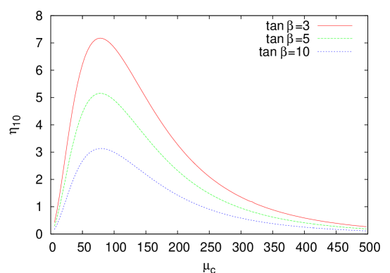
Figure 6: This plot shows $\eta_{10}=10^{10}\eta$ as a function of $\mu_{c}$, $M_{2}=\mu_{c}-20$ GeV, $m_{A}=150$ GeV and for several values of $\tan\beta$.

On the other hand $\tan\beta$ due to the mass of the lightest Higgs is restricted to be in the range Madrid_group

$$5\lesssim\tan\beta$$ (66)

such that we are not allowed to enter the region with smaller values of $\tan\beta$. In addition even for $\tan\beta=3$ our result is still a factor 2 to small. Note that this is a very different conclusion from the one reached in Ref. BalazsCarenaMenonMorrisseyWagner:2004 , where an ample region of parameter space was claimed to result in a successful baryogenesis in the MSSM.

Based on our analysis, can we conclude that the MSSM baryogenesis is ruled out? At least a factor 2 can be accounted for based on the inaccuracies in the parameters in diffusion equations, as well as from approximations that lead to the set of diffusion equations considered here, but unlikely a factor 5 ClineJoyceKainulainen:2000 . Nevertheless, it would be premature to claim that the MSSM baryogenesis is ruled out, since the chargino mediated baryogenesis studied here does not exhaust the possibilities of the MSSM. Recall that neutralinos mediate baryogenesis as well, and that their contribution may be as important or even more important than that from charginos. Furthermore, in the complete set of diffusion equations, there may be additional channels, which lead to baryon production, as of yet unaccounted for. Finally the EDM analysis given here is not conclusive. For larger values of $m_{A}$ and due to the possibility of fortuitous cancellations between different EDM contributions, the value of the electron EDM could be reduced relative to the generic values used above . Hence electroweak baryogenesis seems to be still possible in the MSSM and in this respect we agree with the conclusion drawn in Madrid_group ; Madrid_group_imp ; BalazsCarenaMenonMorrisseyWagner:2004 . However, we would like to emphasis two robust and novel consequences resulting from the quantum treatment of transport in the chargino sector: The BAU is strongly suppressed away from the chargino mass degeneracy and one requires even close to the degeneracy a CP-violating phase of order unity, more precisely $\textrm{arg}(M_{2}\mu_{c})>0.2$.

Modifications of the MSSM with an additional singlet (NMSSM) also contain the prominent chargino channels. As shown in Huber:1998ck ; Huber:1999sa one easily can get a strong first order phase transition and also spontaneous CP-violation at the temperature $T_{c}$ of the phase transition not affecting the EDM at $T=0$. This then allows for a satisfying baryon asymmetry without squeezing the (unfortunately many) parameters. One can also think about extensions of the MSSM that not forbid $\tan\beta\sim 1$ Han:2004yd or modifications of the Standard Model Bodeker:2004ws , where the chargino system does not appear, but of course again quantum-transport is important.

In summary, our numerical solution to the diffusion equations (51–54) shows that a successful baryogenesis at the electroweak scale from charginos of the MSSM is possible only when CP violation is quite large, and near the resonance, $|\mu_{c}-M_{2}|\ll 50\textrm{ GeV}$, $M_{2},\mu_{c}\ll 500$ GeV. As long as the first order sources dominate, due to the oscillations, this picture persists also for much stronger sources, which is to be contrasted to Madrid_group ; Madrid_group_imp ; BalazsCarenaMenonMorrisseyWagner:2004 .

Our conclusion is that, in purely chargino mediated MSSM baryogenesis the capability to explain the observed baryon asymmetry is strongly constrained by the current electron EDM bounds.

Appendix A Comparison of Bosonic Sources

In this Appendix we show how the sources, presented in the current work, relate with those of references Madrid_group ; Madrid_group_imp in the bosonic case and in the limit of zero widths . In order to inspect this we make use of the Kadanoff-Baym equations for the full $2\times 2$ Green functions of the Schwinger-Keldysh formalism. These equations are obtained from Eqs. (11–12) if we substitute $\Delta^{<}$ by the full $2\times 2$ propagator,

$$\Delta=\left(\begin{array}[]{cc}\Delta^{++}&\Delta^{+-}\cr\Delta^{-+}&\Delta^{--}\cr\end{array}\right)=\left(\begin{array}[]{cc}\Delta^{t}&\Delta^{<}\cr\Delta^{>}&\Delta^{\bar{t}}\cr\end{array}\right)\,,$$ (67)

insert unity in the r.h.s. of (11), and set the collision term of (12) to zero,

$$\left(k^{2}-\frac{1}{4}\partial^{2}_{X}\right)\Delta-\frac{1}{2}\left\{{\cal M}^{2},\Delta\right\}+\frac{i}{4}\left[\partial_{\mu}^{X}{\cal M}^{2},\partial_{k}^{\mu}\Delta\right] =1$$ (68)

$$k\cdot\partial_{X}\Delta+\frac{i}{2}\left[{\cal M}^{2},\Delta\right]+\frac{1}{4}\left\{\partial_{\mu}^{X}{\cal M}^{2},\partial_{k}^{\mu}\Delta\right\} =0\,.$$ (69)

In Madrid_group the corresponding Dyson-Schwinger equation for $\Delta$ is iteratively solved as an expansion in powers of $\partial_{\mu}^{X}{\cal M}^{2}$,

$$\Delta=\Delta^{(0)}+\Delta^{(1)}+\dots$$ (70)

where $\Delta^{(0)}$ is the leading order equilibrium propagator, and $\Delta^{(1)}={\cal O}(\partial_{\mu}^{X}{\cal M}^{2})$ denotes a first order correction. Upon performing a Wigner transform over the spatial variables, $\int d^{4}(x-y)\,{\rm e}^{i(x-y)\cdot k}$, identifying $z=(x+y)/2\equiv X$, and transforming into the flavour basis, the first order correction, $\Delta^{(1)}=\Delta^{(1)}(k;X)$ given in Eq. (2.5) of Ref. Madrid_group becomes

$$\Delta^{(1)}=\frac{i}{2}\left[(\partial_{k}^{\mu}\Delta^{(0)})(\partial_{\mu}^{X}{\cal M}^{2})\Delta^{(0)}-\Delta^{(0)}(\partial_{\mu}^{X}{\cal M}^{2})\partial_{k}^{\mu}\Delta^{(0)}\right]\,.$$ (71)

In the approach advocated in Madrid_group in the calculation of the sources one is not interested in long range effects, and hence the term $\partial_{X}^{2}\Delta^{(1)}$ in the constraint equation (68) and $k\cdot\partial_{X}\Delta^{(1)}$ in (69) were considered of second order, and thus have been neglected. From Ref. fermions and this work we know however that, when the dynamics is taken account of, in the case of mixing scalars and fermions the flavour oscillations mess up the derivative expansion, such that only the terms containing spatial derivatives acting on the mass term are genuinely derivative-suppressed.

Upon inserting (70) into (68–69) and using the prescription for derivative counting of Madrid_group , we get for the leading order propagator,

$$k^{2}\Delta^{(0)}-\frac{1}{2}\big{\{}{\cal M}^{2},\Delta^{(0)}\big{\}}=1\,,$$ (72)

which is solved by the thermal Green function, which commutes with ${\cal M}^{2}$. The first order equations are,

$$k^{2}\Delta^{(1)}-\frac{1}{2}\left\{{\cal M}^{2},\Delta^{(1)}\right\}+\frac{i}{4}\left[\partial_{\mu}^{X}{\cal M}^{2},\partial_{k}^{\mu}\Delta^{(0)}\right] = 0$$ (73)

$$k\cdot\partial_{X}\Delta^{(0)}+\frac{i}{2}\left[{\cal M}^{2},\Delta^{(1)}\right]+\frac{1}{4}\left\{\partial_{\mu}^{X}{\cal M}^{2},\partial_{k}^{\mu}\Delta^{(0)}\right\} = 0\,.$$ (74)

By a judicious use of (72) and its derivatives,

$$(k^{2}-{\cal M}^{2})\Delta^{(0)} = 1=\Delta^{(0)}(k^{2}-{\cal M}^{2})$$

$$(k^{2}-{\cal M}^{2})\partial_{\mu}^{X}\Delta^{(0)} = (\partial_{\mu}^{X}{\cal M}^{2})\Delta^{(0)}\,,\qquad(\partial_{\mu}^{X}\Delta^{(0)})(k^{2}-{\cal M}^{2})=\Delta^{(0)}(\partial_{\mu}^{X}{\cal M}^{2})$$

$$(k^{2}-{\cal M}^{2})\partial^{\mu}_{k}\Delta^{(0)} = -(2k^{\mu})\Delta^{(0)}=(\partial^{\mu}_{k}\Delta^{(0)})(k^{2}-{\cal M}^{2})\,$$ (75)

one finds that the first order correction (71) can be recast as,

$$\Delta^{(1)} = \frac{i}{2}\left[(\partial_{k}^{\mu}\Delta^{(0)})(k^{2}-{\cal M}^{2})\partial_{\mu}^{X}\Delta^{(0)}-(\partial_{\mu}^{X}\Delta^{(0)})(k^{2}-{\cal M}^{2})\partial_{k}^{\mu}\Delta^{(0)}\right]$$ (76)

$$= -i\left[\Delta^{(0)}k\cdot\partial_{X}\Delta^{(0)}-(k\cdot\partial_{X}\Delta^{(0)})\Delta^{(0)}\right]\,.$$

It can be easily shown that, when this is inserted into (73–74), one obtains two consistent equations for $\Delta^{(1)}$.

Note that taking moments of the kinetic equation (74) allows for a simple prescription on how the CP-violating source originally calculated in Madrid_group enters the relevant transport equations for squarks. The term $\Delta^{(1)}$ enters through the commutator $[{\cal M}^{2},\Delta^{(1)}]$ in (74), while Madrid_group used a heuristic prescription for the sources based on the Fick’s law and interpreted the diagonal entries of $\Delta^{(1)}$ in the interaction basis as sources for the classical diffusion equations.

Note further that, even though we have rephrased the source of Madrid_group in our language, it remains a nontrivial matter to establish the exact correspondence between the source of Madrid_group appearing in (74) and the source calculated in this work. Our source is in principle obtained by the means of the kernel of Eq. (33) acting upon (34), which is thus of a complicated nonlocal form, and bares no simple relation to the source in (74), apart from a rather superficial similarity, stemming from the fact that the kernel of Eq. (33) is a nonlocal functional of the commutator $[{\cal M}^{2}(z^{\prime}),\cdot]$ acting upon (34) (see Ref. fermions ).

Finally, we emphasize that the difference in how the sources couple to the diffusion equations cannot alone explain a different baryon asymmetry obtained by the two methods, but also the presence of the oscillatory terms.

As regards the case of mixing fermions, we expect that the sources can be related in a similar fashion. Because of the spinor structure however, the comparison for fermions is a nontrivial generalization of the bosonic case.

References

- (1) T. Konstandin, T. Prokopec and M. G. Schmidt, “Kinetic description of fermion flavor mixing and CP-violating sources for baryogenesis,” Nucl. Phys. B 716 (2005) 373 [arXiv:hep-ph/0410135].
- (2) V. A. Kuzmin, V. A. Rubakov and M. E. Shaposhnikov, “On The Anomalous Electroweak Baryon Number Nonconservation In The Early Universe,” Phys. Lett. B 155 (1985) 36. M. E. Shaposhnikov, “Electroweak baryogenesis,” Contemp. Phys. 39 (1998) 177.
- (3) K. Kajantie, M. Laine, K. Rummukainen and M. E. Shaposhnikov, “A non-perturbative analysis of the finite T phase transition in SU(2) x U(1) electroweak theory,” Nucl. Phys. B 493 (1997) 413 [arXiv:hep-lat/9612006].
- (4) F. Csikor, Z. Fodor and J. Heitger, “Endpoint of the hot electroweak phase transition,” Phys. Rev. Lett. 82 (1999) 21 [arXiv:hep-ph/9809291].
- (5) M. Carena, M. Quiros and C. E. M. Wagner, “Opening the Window for Electroweak Baryogenesis,” Phys. Lett. B 380 (1996) 81 [arXiv:hep-ph/9603420]. J. R. Espinosa, “Dominant Two-Loop Corrections to the MSSM Finite Temperature Effective Potential,” Nucl. Phys. B 475 (1996) 273 [arXiv:hep-ph/9604320]. B. de Carlos and J. R. Espinosa, “The baryogenesis window in the MSSM,” Nucl. Phys. B 503 (1997) 24 [arXiv:hep-ph/9703212].
- (6) D. Bodeker, P. John, M. Laine and M. G. Schmidt, “The 2-loop MSSM finite temperature effective potential with stop condensation,” Nucl. Phys. B 497 (1997) 387 [arXiv:hep-ph/9612364]. M. Laine and K. Rummukainen, “The MSSM electroweak phase transition on the lattice,” Nucl. Phys. B 535 (1998) 423 [arXiv:hep-lat/9804019].
- (7) M. Joyce, T. Prokopec and N. Turok, “Electroweak baryogenesis from a classical force,” Phys. Rev. Lett. 75 (1995) 1695 [Erratum-ibid. 75 (1995) 3375] [arXiv:hep-ph/9408339]. M. Joyce, T. Prokopec and N. Turok, “Nonlocal electroweak baryogenesis. Part 2: The Classical regime,” Phys. Rev. D 53 (1996) 2958 [arXiv:hep-ph/9410282].
- (8) J. M. Cline, M. Joyce and K. Kainulainen, “Supersymmetric electroweak baryogenesis in the WKB approximation,” Phys. Lett. B 417 (1998) 79 [Erratum-ibid. B 448 (1998) 321] [arXiv:hep-ph/9708393].
- (9) N. Rius and V. Sanz, “Supersymmetric electroweak baryogenesis,” Nucl. Phys. B 570 (2000) 155 [arXiv:hep-ph/9907460].
- (10) J. M. Cline, M. Joyce and K. Kainulainen, “Supersymmetric electroweak baryogenesis,” JHEP 0007 (2000) 018 [arXiv:hep-ph/0006119]. [Erratum-ibid, arXiv:hep-ph/0110031].
- (11) S. J. Huber and M. G. Schmidt “Electroweak baryogenesis: Concrete in a SUSY model with a gauge singlet,” Nucl. Phys. B 606 (2001) 183 [arXiv:hep-ph/0003122]; S. J. Huber, P. John and M. G. Schmidt, “Bubble walls, CP violation and electroweak baryogenesis in the MSSM,” Eur. Phys. J. C 20, 695 (2001) [arXiv:hep-ph/0101249]. J. Kang, P. Langacker, T. j. Li and T. Liu, “Electroweak baryogenesis in a supersymmetric U(1)’ model,” Phys. Rev. Lett. 94 (2005) 061801 [arXiv:hep-ph/0402086].
- (12) J. Bhatt and R. Rangarajan, “Studying electroweak baryogenesis using evenisation and the Wigner formalism,” JHEP 0503, 057 (2005) [arXiv:hep-ph/0412108].
- (13) M. Carena, J. M. Moreno, M. Quirós, M. Seco and C. E. Wagner, “Supersymmetric CP-violating currents and electroweak baryogenesis,” Nucl. Phys. B 599 (2001) 158 [arXiv:hep-ph/0011055].
- (14) M. Carena, M. Quirós, M. Seco and C. E. M. Wagner, “Improved results in supersymmetric electroweak baryogenesis,” Nucl. Phys. B 650 (2003) 24 [arXiv:hep-ph/0208043].
- (15) C. Balazs, M. Carena, A. Menon, D. E. Morrissey and C. E. M. Wagner, “The supersymmetric origin of matter,” Phys. Rev. D 71 (2005) 075002 [arXiv:hep-ph/0412264].
- (16) P. Huet and A. E. Nelson, “Electroweak baryogenesis in supersymmetric models,” Phys. Rev. D 53 (1996) 4578 [arXiv:hep-ph/9504427].
- (17) K. Kainulainen, T. Prokopec, M. G. Schmidt and S. Weinstock, “First principle derivation of semiclassical force for electroweak baryogenesis,” JHEP 0106 (2001) 031 [arXiv:hep-ph/0105295]. K. Kainulainen, T. Prokopec, M. G. Schmidt and S. Weinstock, “Semiclassical force for electroweak baryogenesis: Three-dimensional derivation,” Phys. Rev. D 66 (2002) 043502 [arXiv:hep-ph/0202177].
- (18) T. Prokopec, M. G. Schmidt and S. Weinstock, “Transport equations for chiral fermions to order h-bar and electroweak baryogenesis: Part I,” Annals Phys. 314 (2004) 208 [arXiv:hep-ph/0312110]. T. Prokopec, M. G. Schmidt and S. Weinstock, “Transport equations for chiral fermions to order h-bar and electroweak baryogenesis: Part II,” Annals Phys. 314 (2004) 267 [arXiv:hep-ph/0406140].
- (19) J. M. Cline and K. Kainulainen, “A new source for electroweak baryogenesis in the MSSM,” Phys. Rev. Lett. 85 (2000) 5519 [arXiv:hep-ph/0002272].
- (20) M. Carena, M. Quiros, A. Riotto, I. Vilja and C. E. M. Wagner, “Electroweak baryogenesis and low energy supersymmetry,” Nucl. Phys. B 503 (1997) 387 [arXiv:hep-ph/9702409].
- (21) M. Joyce, T. Prokopec and N. Turok, “Nonlocal electroweak baryogenesis. Part 1: Thin wall regime,” Phys. Rev. D 53 (1996) 2930 [arXiv:hep-ph/9410281].
- (22) D. Bodeker, “On the effective dynamics of soft non-abelian gauge fields at finite temperature,” Phys. Lett. B 426 (1998) 351 [arXiv:hep-ph/9801430]. G. D. Moore, “The sphaleron rate: Boedeker’s leading log,” Nucl. Phys. B 568 (2000) 367 [arXiv:hep-ph/9810313]. D. Bödeker, G. D. Moore and K. Rummukainen, “Chern-Simons number diffusion and hard thermal loops on the lattice,” Phys. Rev. D 61 (2000) 056003 [arXiv:hep-ph/9907545].
- (23) G. F. Giudice and M. E. Shaposhnikov, “Strong sphalerons and electroweak baryogenesis,” Phys. Lett. B 326 (1994) 118 [arXiv:hep-ph/9311367].
- (24) M. Carena, M. Quiros and C. E. M. Wagner, “Electroweak baryogenesis and Higgs and stop searches at LEP and the Tevatron,” Nucl. Phys. B 524 (1998) 3 [arXiv:hep-ph/9710401].
- (25) J. M. Moreno, M. Quirós and M. Seco, “Bubbles in the supersymmetric standard model,” Nucl. Phys. B 526 (1998) 489 [arXiv:hep-ph/9801272].
- (26) A. Riotto, “The more relaxed supersymmetric electroweak baryogenesis,” Phys. Rev. D 58 (1998) 095009 [arXiv:hep-ph/9803357].
- (27) Tomislav Prokopec, Michael G. Schmidt and Steffen Weinstock, “Transport equations for chiral fermions to order and electroweak baryogenesis,” to appear in the proceedings of the International Workshop ”Strong and Electroweak Matter 2004” (SEWM04), Helsinki, Finland, 16-19 Jun 2004, preprint ITP-UU-04/28, SPIN-04/16.
- (28) K. Kainulainen, T. Prokopec, M. G. Schmidt and S. Weinstock, “Some aspects of collisional sources for electroweak baryogenesis,” arXiv:hep-ph/0201245.
- (29) C. Lee, V. Cirigliano and M. J. Ramsey-Musolf, “Resonant relaxation in electroweak baryogenesis,” Phys. Rev. D 71, 075010 (2005) [arXiv:hep-ph/0412354].
- (30) D. Chang, W. F. Chang and W. Y. Keung, “New constraint from electric dipole moments on chargino baryogenesis in MSSM,” Phys. Rev. D 66 (2002) 116008 [arXiv:hep-ph/0205084].
- (31) A. Pilaftsis, “Higgs-mediated electric dipole moments in the MSSM: An application to baryogenesis and Higgs searches,” Nucl. Phys. B 644 (2002) 263 [arXiv:hep-ph/0207277].
- (32) B. C. Regan, E. D. Commins, C. J. Schmidt and D. DeMille, “New limit on the electron electric dipole moment,” Phys. Rev. Lett. 88 (2002) 071805.
- (33) S. J. Huber and M. G. Schmidt, “SUSY variants of the electroweak phase transition,” Eur. Phys. J. C 10, 473 (1999) [arXiv:hep-ph/9809506].
- (34) S. J. Huber, P. John, M. Laine and M. G. Schmidt, “CP violating bubble wall profiles,” Phys. Lett. B 475, 104 (2000) [arXiv:hep-ph/9912278].
- (35) T. Han, P. Langacker and B. McElrath, “The Higgs sector in a U(1)’ extension of the MSSM,” Phys. Rev. D 70, 115006 (2004) [arXiv:hep-ph/0405244].
- (36) D. Bodeker, L. Fromme, S. J. Huber and M. Seniuch, “The baryon asymmetry in the standard model with a low cut-off,” JHEP 0502 (2005) 026 [arXiv:hep-ph/0412366]. C. Grojean, G. Servant and J. D. Wells, “First-order electroweak phase transition in the standard model with a low cutoff,” Phys. Rev. D 71 (2005) 036001 [arXiv:hep-ph/0407019].