Analyticity properties of three-point functions in QCD beyond leading order

Abstract

The removal of unphysical singularities in the perturbatively calculable part of the pion form factor—a classic example of a three-point function in QCD—is discussed. Different “analytization” procedures in the sense of Shirkov and Solovtsov are examined in comparison with standard QCD perturbation theory. We show that demanding the analyticity of the partonic amplitude as a whole, as proposed before by Karanikas and Stefanis, one can make infrared finite not only the strong running coupling and its powers, but also cure potentially large logarithms (that first appear at next-to-leading order) containing the factorization scale and modifying the discontinuity across the cut along the negative real axis. The scheme used here generalizes the Analytic Perturbation Theory of Shirkov and Solovtsov to non-integer powers of the strong coupling and diminishes the dependence of QCD hadronic quantities on all perturbative scheme and scale-setting parameters, including the factorization scale.

I Introduction

The phenomenology of QCD exclusive processes depends in a crucial way on the analytic properties of hadronic (hard) scattering amplitudes as functions of the strong running coupling. A perturbatively calculable short-distance part of the reaction amplitude at the parton level is isolated either by subtraction or by factorization. To get a quantitative interpretation of such quantities in practice and compare them with experimental data, one has to get rid of the artificial Landau singularity at $Q^{2}=\Lambda^{2}_{\text{QCD}}$ ($\Lambda_{\text{QCD}}\equiv\Lambda$ in the following), where $Q^{2}$ is the large mass scale in the process. A proposal to solve this problem (in the spacelike region) without introducing exogenous infrared (IR) regulators, like an effective, or a dynamically generated, gluon mass Cor82 (see, for instance, PP79 ; JSL87 ; Ste89 ; JiAm90 ; SB93D ; MS93 ; BJPR98 ; Mul98 ; Ste99 for such applications), was made by Shirkov and Solovtsov (SS) SS97 ; Shi98 ; SS99 , based on general principles of local Quantum Field Theory. This theoretical framework—termed Analytic Perturbation Theory (APT)—was further expanded beyond the one-loop level of two-point functions to define an analytic coupling and its powers in the timelike region SS98 ; DVS00unp ; Shi00 ; SS01 ; KM01 ; Mag99 ; BMMR02 ; Ale05 , embracing previous attempts Rad82 ; KP82 ; BB94 ; BBB95 ; MS97 ; BRS00 in this direction.

However, first applications SSK99 ; SSK00 of this sort of approach to three-point functions, beyond the leading order of QCD perturbation theory, have made it clear that, ultimately, there must be an extension of this formalism from the level of the running coupling and its powers to the level of amplitudes. The reason is that in three-point functions at the next-to-leading order (NLO) level, and beyond, logarithms of a distinct scale (serving as the factorization or evolution scale) appear that though they do not change the nature of the Landau pole, they affect the discontinuity across the cut along the negative real axis $-\infty<Q^{2}<0$. On account of factorization, we expect that this effect should be small, of the order of a few percent, because any change caused by the variation of the factorization scale should be of the next higher order. However, to achieve a high-precision theoretical prediction, one should reduce this uncertainty, lifting the limitations imposed by the lack of knowledge about uncalculated higher-order corrections. To encompass such logarithmic terms in the “analytization” procedure, one should demand the analyticity of the partonic amplitude as a whole KS01 ; Ste02 and calculate the dispersive image of the coupling (or of its powers) in conjunction with these logarithms. This Karanikas–Stefanis (KS) “analytization” scheme effectively amounts to the generalization of APT to non-integer powers of the running coupling: Fractional APT (FAPT), as we shall show below.

In this work we expand the Shirkov–Solovtsov “analytization” approach to include the dispersive images of such terms, using as a case study the pion form factor at NLO in the $\overline{\text{MS}\vphantom{{}^{1}}}$ scheme with various renormalization-scale settings and also in the $\alpha_{V}$-scheme BrodskyL95 . To this end, we contrast the KS “analytization” with the naive SSK99 ; SSK00 and the maximal BPSS04 “analytization” procedures and work out their key mutual differences as they first appear in NLO, while a fully-fledged analysis of FAPT is given in an accompanying paper BMS05 . We argue that augmenting the $\overline{\text{MS}\vphantom{{}^{1}}}$ scheme with the KS “analytization” prescription provides an optimized method to calculate perturbatively higher-order corrections to partonic “observables” in QCD because it practically eliminates all scheme and scale-setting ambiguities owing to the renormalization and factorization scales. It is worth emphasizing at this point that the focus of Ref. KS01 was on the calculation of power corrections to the pion’s electromagnetic form factor. Such contributions are outside the scope of the present investigation.

The plan of this paper is as follows. In Sec. II we review the convolution formalism for the calculation of the short-distance part of the pion form factor within perturbative QCD at NLO. In Sec. III we discuss the Shirkov–Solovtsov type “analytization” procedures SS97 ; SSK99 ; SSK00 ; KS01 ; Ste02 ; BPSS04 and work out their mutual differences, focusing on the KS “analytization” and its properties. This discussion extends and generalizes the original KS analysis that covered only the LO of the perturbative expansion of the pion form factor and ignoring evolution. Section IV contains the results for the factorized pion form factor in different schemes and with different scale settings, employing the KS “analytization” in comparison with those based on APT and also standard QCD perturbation theory in NLO. Our conclusions with a summary of our main results are presented in Sec. V. Some important technical details are collected in three appendices.

II Factorizable Part of the Pion Form Factor at NLO in Standard QCD Perturbation Theory

The leading-twist factorizable part of the electromagnetic pion form factor can be expressed as a convolution in the form ER80 ; LB80

$$F_{\pi}^{\text{Fact}}(Q^{2};\mu_{\text{R}}^{2})=\Phi_{\pi}^{*}(x,\mu_{\text{F}}^{2})\mathop{\otimes}\limits_{x}T_{\text{H}}(x,y,Q^{2};\mu_{\text{F}}^{2},\mu_{\text{R}}^{2})\mathop{\otimes}\limits_{y}\Phi_{\pi}(y,\mu_{\text{F}}^{2})\,,$$ (1)

where $\otimes$ denotes the usual convolution symbol ($A(z)\mathop{\otimes}\limits_{z}B(z)\equiv\int_{0}^{1}dzA(z)B(z)$) over the longitudinal momentum fraction variable $x$ ($y$) and $\mu_{\text{F}}$ represents the factorization scale at which the separation between the long- (small transverse momentum) and short-distance (large transverse momentum) dynamics takes place, with $\mu_{\text{R}}$ labelling the renormalization (coupling constant) scale. The nonperturbative input is encoded in the pion distribution amplitude (DA) $\Phi_{\pi}(y,\mu_{\text{F}}^{2})$, whereas the short-distance interactions are represented by the hard-scattering amplitude $T_{\text{H}}(x,y,Q^{2};\mu_{\text{F}}^{2},\mu_{\text{R}}^{2})$. This is the amplitude for a collinear valence quark-antiquark pair with total momentum $P$ struck by a virtual photon with momentum $q$, satisfying $q^{2}=-Q^{2}$, to end up again in a configuration of a parallel valence quark-antiquark pair with momentum $P^{\prime}=P+q$. It can be calculated perturbatively in the form of a power-series expansion in the QCD coupling, the latter to be evaluated at the reference scale of renormalization $\mu_{\text{R}}^{2}$:

$$T^{\text{NLO}}_{\text{H}}(x,y,Q^{2};\mu_{\text{F}}^{2},\mu_{\text{R}}^{2})=\alpha_{s}\left(\mu_{\text{R}}^{2}\right)\,T_{\text{H}}^{(0)}(x,y,Q^{2})+\frac{\alpha_{s}^{2}\left(\mu_{\text{R}}^{2}\right)}{4\pi}\,T_{\text{H}}^{(1)}(x,y,Q^{2};\mu_{\text{F}}^{2},\mu_{\text{R}}^{2})\,.$$ (2)

The leading-order (LO) contribution to $T_{\text{H}}(x,y,Q^{2};\mu_{\text{F}}^{2})$ reads

$$T_{\text{H}}^{(0)}(x,y,Q^{2})=\frac{N_{\text{T}}}{Q^{2}}\,\frac{1}{\overline{x}\,\overline{y}\,}\equiv\frac{1}{Q^{2}}\,t_{\text{H}}^{(0)}(x,y)\,,$$ (3)

where

$$N_{\text{T}}=\frac{2\,\pi\,C_{\text{F}}}{C_{\text{A}}}=\frac{8\pi}{9}\,,$$ (4)

$C_{\text{F}}=\left(N_{\text{c}}^{2}-1\right)/2N_{\text{c}}=4/3$, $C_{\text{A}}=N_{\text{c}}=3$ are the color factors of $SU(3)_{\text{c}}$, and the notation $\bar{z}\equiv 1-z$ has been used. The usual color decomposition of the NLO correction MNP98 —marked by self-explainable labels—is given by (omitting the variables $x$ and $y$)

$$Q^{2}T_{\text{H}}^{(1)}\left(Q^{2};\mu_{\text{F}}^{2},\mu_{\text{R}}^{2}\right)=C_{\text{F}}\,t_{\text{H}}^{(1,\text{F})}\left(\frac{\mu_{\text{F}}^{2}}{Q^{2}}\right)+b_{0}\,t_{\text{H}}^{(1,\beta)}\left(\frac{\mu_{\text{R}}^{2}}{Q^{2}}\right)+C_{\text{G}}\,t_{\text{H}}^{(1,\text{G})}\,,$$ (5)

where $C_{\text{G}}=(C_{\text{F}}-C_{\text{A}}/2)$ and $b_{0}$ is the first coefficient of the $\beta$ function, see Appendix A, Eq. (43). Here we explicitly factorized out a trivial $1/Q^{2}$ dependence and used for the coefficients in front of each factor the notation $t_{\text{H}}$ with appropriate superscripts.

With reference to the application of the Brodsky–Lepage–Mackenzie (BLM) BLM83 scale setting in fixing the renormalization point later on, we single out the $b_{0}$-proportional (i.e., the $N_{f}$-dependent) term, given by

$$t_{\text{H}}^{(1,\beta)}\left(x,y;\frac{\mu_{\text{R}}^{2}}{Q^{2}}\right) = t_{\text{H},1}^{(1,\beta)}\left(x,y\right)+t_{\text{H},2}^{(1,\beta)}\left(x,y;\frac{\mu_{\text{R}}^{2}}{Q^{2}}\right)$$ (6a)

with

$$t_{\text{H},1}^{(1,\beta)}\left(x,y\right) = t_{\text{H}}^{(0)}\left(x,y\right)\,\left[\frac{5}{3}-\ln(\overline{x}\,\overline{y}\,)\right]$$ (6b)

$$t_{\text{H},2}^{(1,\beta)}\left(x,y;\frac{\mu_{\text{R}}^{2}}{Q^{2}}\right) = t_{\text{H}}^{(0)}\left(x,y\right)\,\ln\frac{\mu_{\text{R}}^{2}}{Q^{2}}\,,$$ (6c)

and present the color singlet part of $t_{\text{H}}$ in the form

$$t_{\text{H}}^{(1,\text{F})}\left(x,y;\frac{\mu_{\text{F}}^{2}}{Q^{2}}\right) = t_{\text{H},1}^{(1,\text{F})}\left(x,y\right)+t_{\text{H},2}^{(1,\text{F})}\left(x,y;\frac{\mu_{\text{F}}^{2}}{Q^{2}}\right)\,;$$ (7a)

$$t_{\text{H},2}^{(1,\text{F})}\left(x,y;\frac{\mu_{\text{F}}^{2}}{Q^{2}}\right) = t_{\text{H}}^{(0)}\left(x,y\right)\left[2\Big{(}3+\ln(\overline{x}\,\overline{y}\,)\Big{)}\ln\frac{Q^{2}}{\mu_{\text{F}}^{2}}\right]\,.$$ (7b)

Explicit expressions for $t_{\text{H},1}^{(1,\text{F})}\left(x,y\right)$ and for the color non-singlet part, $t_{\text{H}}^{(1,\text{G})}\left(x,y\right)$, cf. Eq. (5), are supplied in Appendix B (see Eqs. (45), (46)).

The scaled hard-scattering amplitude, Eq. (2), truncated at the NLO and evaluated at the renormalization scale $\mu_{\text{R}}^{2}=\lambda_{\text{R}}Q^{2}$, reads

$$Q^{2}T^{\text{NLO}}_{\text{H}}\left(x,y,Q^{2};\mu_{\text{F}}^{2},\lambda_{\text{R}}Q^{2}\right)=\alpha_{s}\left(\lambda_{\text{R}}Q^{2}\right)\,t_{\text{H}}^{(0)}(x,y)+\frac{\alpha_{s}^{2}\left(\lambda_{\text{R}}Q^{2}\right)}{4\pi}\,C_{\text{F}}\,t_{\text{H},2}^{(1,\text{F})}\left(x,y;\frac{\mu_{\text{F}}^{2}}{Q^{2}}\right)~{}~{}~{}$$

$$+\ \frac{\alpha_{s}^{2}\left(\lambda_{\text{R}}Q^{2}\right)}{4\pi}\left\{b_{0}\,t_{\text{H}}^{(1,\beta)}(x,y;\lambda_{\text{R}})+t_{\text{H}}^{(\text{FG})}(x,y)\right\}\,,~{}~{}~{}~{}~{}~{}~{}~{}~{}~{}~{}~{}~{}~{}$$ (8)

where we have introduced the shorthand notation

$$t_{\text{H}}^{(\text{FG})}(x,y)\equiv C_{\text{F}}\,t_{\text{H},1}^{(1,\text{F})}(x,y)+C_{\text{G}}\,t_{\text{H}}^{(1,\text{G})}(x,y)\,.$$ (9)

To calculate the factorizable part of the pion form factor, one has to convolute this expression with the pion DA for each hadron in the initial and final state. In leading twist 2, the pion DA at the normalization scale ${\mu_{0}^{2}}\approx 1$ GeV² is given by

$$\varphi_{\pi}(x,\mu_{0}^{2})=6x(1-x)\left[1+a_{2}({\mu_{0}^{2}})\,C_{2}^{3/2}(2x-1)+a_{4}({\mu_{0}^{2}})\,C_{4}^{3/2}(2x-1)+\ldots\right]\,,$$ (10)

with all nonperturbative information being encapsulated in the Gegenbauer coefficients $a_{n}$. In this analysis we use those coefficients determined before by Bakulev, Mikhailov, and Stefanis (BMS) in BMS01 with the aid of QCD sum rules with nonlocal condensates:

$$a_{2}^{\rm BMS}=0.20,\quad a_{4}^{\rm BMS}=-0.14,\quad a_{n}^{\rm BMS}=0\>,n>4\,,$$ (11)

where the vacuum quark virtuality $\lambda_{q}^{2}=0.4$ GeV² has been used. This set of values was found BMS02 ; BMS03 to be consistent at the $1\sigma$ level with the high-precision CLEO data CLEO98 on the pion-photon transition form factor, with all other model DAs being outside—at least—the $2\sigma$ error ellipse (see BMS04kg for the latest compilation of models in comparison with the CLEO and CELLO CELLO91 data). Notice that the particular parameterization (shape) of the pion DA chosen is irrelevant for the considerations to follow.

III Analyticity of Partonic Amplitudes Beyond LO

III.1 Analytic Running Coupling in QCD

The main stumbling block in applying fixed-order perturbation theory at low momenta $Q^{2}$ is the non-physical Landau singularity of the running strong coupling at $Q^{2}=\Lambda^{2}$, which entails the appearance of IR renormalons in the perturbative expansion. To ensure the analyticity of the coupling in the infrared, one can follow different strategies CS93 ; BBB95 ; DMW96 ; SS97 ; CMNT96 ; Magn00 ; BRS00 ; Gar01 all based on the basic assumption that the physical coupling should stay IR finite and analytic in the whole momentum range, though its precise value at $Q^{2}=0$ is still a matter of debate SS97 ; Nes03 ; Ale05 ; AS00 ; BP04 . Imposing the analyticity of the coupling in the sense of Shirkov and Solovtsov SS97 , we replace the strong running coupling and its powers by their analytic versions:

$$\left[\alpha_{s}^{(n)}\left(Q^{2}\right)^{m}\right]^{\text{an}}\equiv{\cal A}_{m}^{(n)}\left(Q^{2}\right)~{}~{}\text{with}~{}~{}\left[f\left(Q^{2}\right)\right]^{\text{an}}=\frac{1}{\pi}\int_{0}^{\infty}\!\frac{\textbf{Im}\,\big{[}f(-\sigma)\big{]}}{\sigma+Q^{2}-i\epsilon}\,d\sigma\,,$$ (12)

where the loop order is explicitly indicated by the superscript $n$ in parenthesis and

$${\cal A}_{1}^{(1)}\left(Q^{2}\right)=\frac{4\pi}{b_{0}}\left[\frac{1}{\ln(Q^{2}/\Lambda^{2})}+\frac{\Lambda^{2}}{\Lambda^{2}-Q^{2}}\right]\equiv\bar{\alpha}_{s}\left(Q^{2}\right)\,,$$ (13)

with the last step connecting to the SS notation SS97 , and $\alpha_{s}(0)=4\pi/b_{0}$. The two-loop running coupling in standard QCD perturbation theory can be expressed Mag99 in terms of the Lambert function $W_{-1}$ to read

$$\alpha_{s}^{(2)}\left(Q^{2}\right)=-\frac{4\pi}{b_{0}c_{1}}\left[1+W_{-1}\left(-\frac{1}{c_{1}e}\left(\frac{\Lambda^{2}}{Q^{2}}\right)^{1/c_{1}}\right)\right]^{-1}\,.$$ (14)

For some more explanations we refer the interested reader to BMS02 , Appendix C, Eqs. (C15) and (C20). Then, the analytic image of the $k$th power of the coupling DVS00unp is obtained from the dispersion relation

$${\cal A}_{k}^{(2)}\left(Q^{2}\right)=\frac{1}{\pi}\int_{0}^{\infty}d\sigma\frac{\rho_{k}^{(2)}(\sigma)}{\sigma+Q^{2}-i\epsilon}\,$$ (15)

with the spectral density

$$\rho_{k}^{(2)}(t)=\left(\frac{4\pi}{b_{0}c_{1}}\right)^{k}{\textbf{Im}{}}\left(-\frac{1}{1+W_{1}(z(t))}\right)^{k}\,.$$ (16)

In the numerical calculations below, we use an approximate form suggested in BPSS04 :

$${\cal A}_{1}^{(2,\text{fit})}\left(Q^{2}\right) = \frac{4\pi}{b_{0}}\,\left\{\frac{1}{\ell\left[\ln\left(Q^{2}/\Lambda_{21}^{2}\right),\,c_{21}^{\text{fit}}\right]}+\frac{1}{1-\exp(\ell\left[\ln\left(Q^{2}/\Lambda_{21}^{2}\right),\,c_{21}^{\text{fit}}\right])}\right\}\,;$$ (17)

$${\cal A}_{2}^{(2,\text{fit})}\left(Q^{2}\right) = \left(\frac{4\pi}{b_{0}}\right)^{2}\left\{\frac{1}{\ell\left[\ln\left(Q^{2}/\Lambda_{22}^{2}\right),c_{22}^{\text{fit}}\right]^{2}}-\frac{\exp(\ell\left[\ln\left(Q^{2}/\Lambda_{22}^{2}\right),c_{22}^{\text{fit}}\right])}{\left[1-\exp(\ell\left[\ln\left(Q^{2}/\Lambda_{22}^{2}\right),c_{22}^{\text{fit}}\right])\right]^{2}}\right\}\,,~{}~{}~{}$$ (18)

where the values of the fit parameters are listed in Table 1 and

$$\ell[L,c]\equiv L+c\,\ln\sqrt{L^{2}+4\pi^{2}}\,.$$ (19)

Table 1: Parameters entering Eqs. (17) and (18) for the value $\Lambda_{\text{QCD}}^{N_{f}=3}=400$ MeV.

Parameters	$c_{21}^{\text{fit}}$	$\Lambda_{21}$	$c_{22}^{\text{fit}}$	$\Lambda_{22}$
Values	$-1.015$	$67$ MeV	$-1.544$	$34.5$ MeV

III.2 “Analytization” Procedures

Let us now see how analyticity can be implemented on the parton-level pion form factor in NLO accuracy of perturbative QCD. We discuss three “analytization” procedures:

• Naive “analytization” SSK99 ; SSK00 ; BPSS04

  $$\left[Q^{2}T_{\text{H}}\left(x,y,Q^{2};\mu_{\text{F}}^{2},\lambda_{\text{R}}Q^{2}\right)\right]_{\text{SS}}^{\text{naive-an}}={\cal A}_{1}^{(2)}(\lambda_{\text{R}}Q^{2})\,t_{\text{H}}^{(0)}(x,y)~{}~{}~{}~{}~{}~{}~{}~{}~{}~{}~{}~{}~{}~{}~{}~{}~{}~{}~{}~{}~{}~{}~{}~{}~{}~{}~{}~{}~{}$$

  $$+\frac{\left({\cal A}_{1}^{(2)}(\lambda_{\text{R}}Q^{2})\right)^{2}}{4\pi}\,\left[b_{0}\,t_{\text{H}}^{(1,\beta)}(x,y;\lambda_{\text{R}})+t_{\text{H}}^{(\text{FG})}(x,y)+C_{\text{F}}\,t_{\text{H},2}^{(1,\text{F})}\left(x,y;\frac{\mu_{\text{F}}^{2}}{Q^{2}}\right)\right]\,.~{}~{}~{}~{}~{}$$ (20)

• Maximal “analytization” BPSS04

  $$\left[Q^{2}T_{\text{H}}\left(x,y,Q^{2};\mu_{\text{F}}^{2},\lambda_{\text{R}}Q^{2}\right)\right]_{\text{SS}}^{\text{max-an}}={\cal A}_{1}^{(2)}(\lambda_{\text{R}}Q^{2})\,t_{\text{H}}^{(0)}(x,y)~{}~{}~{}~{}~{}~{}~{}~{}~{}~{}~{}~{}~{}~{}~{}~{}~{}~{}~{}~{}~{}~{}~{}~{}~{}~{}~{}~{}~{}~{}~{}~{}~{}~{}~{}$$

  $$+\frac{{\cal A}_{2}^{(2)}(\lambda_{\text{R}}Q^{2})}{4\pi}\,\left[b_{0}\,t_{\text{H}}^{(1,\beta)}(x,y;\lambda_{\text{R}})+t_{\text{H}}^{(\text{FG})}(x,y)+C_{\text{F}}\,t_{\text{H},2}^{(1,\text{F})}\left(x,y;\frac{\mu_{\text{F}}^{2}}{Q^{2}}\right)\right]\,.~{}~{}~{}~{}~{}$$ (21)

• Amplitude “analytization” proposed by Karanikas and Stefanis in KS01 ; Ste02 .

The first method replaces $\alpha_{s}$ and its powers by the Shirkov–Solovtsov analytic coupling SS97 and its powers, whereas the second one uses for the powers of $\alpha_{s}$ their own analytic images, transforming this way the power-series expansion in $[\alpha_{s}\left(Q^{2}\right)]^{n}$ in a functional expansion in terms of the functions ${\cal A}_{n}\left(Q^{2}\right)$ SS99 ; Shi00 . Imposing analyticity in the sense of Karanikas–Stefanis KS01 , differs from the previous two approaches in that it demands the whole partonic amplitude has the correct analytical behavior as a function of $Q^{2}$. This entails the “analytization” of terms of the form $\left(\alpha_{s}^{(n)}\left(Q^{2}\right)\right)^{m}\ln(Q^{2}/\mu_{\rm F}^{2})$, which appear in exclusive amplitudes at NLO of QCD perturbation theory and contain an additional scale, $\mu_{\rm F}^{2}$. There are, in principle, two possibilities how to proceed any further. One option is provided by setting $\mu_{\text{F}}^{2}\simeq Q^{2}$ and then face the problem of “analytization” of terms like $\left[\alpha_{s}\left(Q^{2}\right)/\alpha_{s}({\mu_{0}^{2}})\right]^{\eta}$, where $\eta=\gamma_{n}^{(0)}/(2b_{0})$ is a fractional number, as discussed in BMS05 . Another possibility is to fix the factorization scale $\mu_{\text{F}}^{2}$ at some value and then to redefine the original Shirkov–Solovtsov “analytization” procedure in order to take the dispersive image of the coupling (or of its powers) together with these logarithmic terms. This second route is followed in the present work. It is important to note that the KS “analytization” procedure reduces in LO of fixed-order perturbation theory to the maximal one, as shown in KS01 , provided evolution effects of the pion distribution amplitudes are ignored.

Applying now this generalized “analytization” concept, we get

$$\left[Q^{2}T_{\text{H}}\left(x,y,Q^{2};\mu_{\text{F}}^{2},\lambda_{\text{R}}Q^{2}\right)\right]_{\text{KS}}^{\text{an}}={\cal A}_{1}^{(2)}(\lambda_{\text{R}}Q^{2})\,t_{\text{H}}^{(0)}(x,y)~{}~{}~{}~{}~{}~{}~{}~{}~{}~{}~{}~{}~{}~{}~{}~{}~{}~{}~{}~{}~{}~{}~{}~{}~{}~{}~{}~{}~{}~{}~{}~{}~{}~{}~{}~{}~{}~{}~{}~{}~{}~{}~{}~{}~{}$$

$$+\ \frac{{\cal A}_{2}^{(2)}(\lambda_{\text{R}}Q^{2})}{4\pi}\,\left(b_{0}\,t_{\text{H}}^{(1,\beta)}(x,y;\lambda_{\text{R}})+t_{\text{H}}^{(\text{FG})}(x,y)\right)~{}~{}~{}~{}~{}~{}~{}~{}~{}~{}~{}~{}~{}$$

$$+\left[\frac{\left(\alpha_{s}^{(2)}(\lambda_{\text{R}}Q^{2})\right)^{2}}{4\pi}\,C_{\text{F}}\,t_{\text{H}}^{(0)}(x,y)\left(6+2\ln(\overline{x}\,\overline{y}\,)\right)\ln\frac{Q^{2}}{\mu_{\text{F}}^{2}}\right]_{\text{KS}}^{\text{an}}.~{}~{}~{}~{}$$ (22)

In order to have the same scale argument in the logarithmic term as in the running coupling, we substitute $\ln(Q^{2}/\mu_{\text{F}}^{2})=\ln(\lambda_{\text{R}}Q^{2}/\Lambda^{2})-\ln(\lambda_{\text{R}}\mu_{\text{F}}^{2}/\Lambda^{2})$ to obtain

$$\left[Q^{2}T_{\text{H}}\left(x,y,Q^{2};\mu_{\text{F}}^{2},\lambda_{\text{R}}Q^{2}\right)\right]_{\text{KS}}^{\text{an}}={\cal A}_{1}^{(2)}(\lambda_{\text{R}}Q^{2})\,t_{\text{H}}^{(0)}(x,y)~{}~{}~{}~{}~{}~{}~{}~{}~{}~{}~{}~{}~{}~{}~{}~{}~{}~{}~{}~{}~{}~{}~{}~{}~{}~{}~{}~{}~{}~{}~{}~{}~{}~{}~{}~{}~{}~{}~{}~{}~{}~{}~{}~{}$$

$$~{}~{}~{}~{}~{}+\ \frac{{\cal A}_{2}^{(2)}(\lambda_{\text{R}}Q^{2})}{4\pi}\,\left[b_{0}\,t_{\text{H}}^{(1,\beta)}(x,y;\lambda_{\text{R}})+t_{\text{H}}^{(\text{FG})}(x,y)-C_{\text{F}}\,t_{\text{H}}^{(0)}(x,y)\left(6+2\ln(\overline{x}\,\overline{y}\,)\right)\ln\frac{\lambda_{\text{R}}\mu_{\text{F}}^{2}}{\Lambda^{2}}\right]$$

$$+\ \left[\frac{\left(\alpha_{s}^{(2)}(\lambda_{\text{R}}Q^{2})\right)^{2}}{4\pi}\,C_{\text{F}}\,t_{\text{H}}^{(0)}(x,y)\left(6+2\ln(\overline{x}\,\overline{y}\,)\right)\ln\frac{\lambda_{\text{R}}Q^{2}}{\Lambda^{2}}\right]_{\text{KS}}^{\text{an}}.~{}~{}~{}~{}~{}~{}~{}~{}~{}~{}~{}~{}~{}~{}~{}~{}~{}~{}~{}~{}~{}~{}~{}~{}~{}~{}~{}~{}~{}~{}~{}~{}\$$ (23)

Finally, we arrive at

$$\left[Q^{2}T_{\text{H}}(x,y,Q^{2};\mu_{\text{F}}^{2},\lambda_{\text{R}}Q^{2})\right]_{\text{KS}}^{\text{an}}={\cal A}_{1}^{(2)}(\lambda_{\text{R}}Q^{2})\,t_{\text{H}}^{(0)}(x,y)~{}~{}~{}~{}~{}~{}~{}~{}~{}~{}~{}~{}~{}~{}~{}~{}~{}~{}~{}~{}~{}~{}~{}~{}~{}~{}~{}~{}~{}~{}~{}~{}~{}~{}~{}~{}~{}~{}~{}~{}~{}~{}~{}~{}~{}~{}$$

$$~{}~{}~{}~{}+\ \frac{{\cal A}_{2}^{(2)}(\lambda_{\text{R}}Q^{2})}{4\pi}\,\left[b_{0}\,t_{\text{H}}^{(1,\beta)}(x,y;\lambda_{\text{R}})+t_{\text{H}}^{(\text{FG})}(x,y)+C_{\text{F}}\,t_{\text{H},2}^{(1,\text{F})}\left(x,y;\frac{\mu_{\text{F}}^{2}}{Q^{2}}\right)\right]$$

$$+\ \frac{\Delta_{2}^{(2)}\left(\lambda_{\text{R}}Q^{2}\right)}{4\pi}\,\left[C_{\text{F}}\,t_{\text{H}}^{(0)}(x,y)\,\left(6+2\ln(\bar{x}\bar{y})\right)\right]\,,~{}~{}~{}~{}~{}~{}~{}~{}~{}~{}~{}~{}~{}~{}~{}~{}~{}~{}~{}~{}~{}~{}~{}~{}~{}~{}~{}~{}~{}~{}~{}$$ (24)

where the deviation from Eq. (21) is encoded in the term

$$\Delta_{2}^{(2)}\left(Q^{2}\right) \equiv {\cal L}_{2}^{(2)}\left(Q^{2}\right)-{\cal A}_{2}^{(2)}\left(Q^{2}\right)\,\ln\left[Q^{2}/\Lambda^{2}\right]$$ (25)

with

$${\cal L}_{2}^{(2)}\left(Q^{2}\right) \equiv \left[\left(\alpha_{s}^{(2)}\left(Q^{2}\right)\right)^{2}\ln\left(\frac{Q^{2}}{\Lambda^{2}}\right)\right]_{\text{KS}}^{\text{an}}=\frac{4\pi}{b_{0}}\,\left[\frac{\left(\alpha_{s}^{(2)}\left(Q^{2}\right)\right)^{2}}{\alpha_{s}^{(1)}\left(Q^{2}\right)}\right]_{\text{KS}}^{\text{an}}\,.$$ (26)

It is important to distinguish between the two contributions in Eq. (25). The first amounts to the “analytization” of the product of the coupling with a logarithm, or equivalently of fractional powers of the coupling, as shown in BMS05 . The second bears an additional logarithmic dependence on the momentum scale $Q^{2}$ relative to the expression obtained with the maximal “analytization” procedure. The subscript KS in the last equation signifies that this expression should be analyticized according to the KS prescription. To obtain a clearer idea of its meaning and demonstrate its essence, the “analytization” is performed in three incremental steps. First, a simplified version of this expression is considered, which results by provisionally replacing the two-loop coupling in the numerator by its one-loop counterpart. Then, the ratio of the couplings after “analytization” reduces to (dash-dotted line in Fig. 1a)

$${\cal L}_{2}^{(1)\,\text{approx}}\left(Q^{2}\right)=\frac{4\pi}{b_{0}}\,{\cal A}_{1}^{(1)}\left(Q^{2}\right)\,.$$ (27)

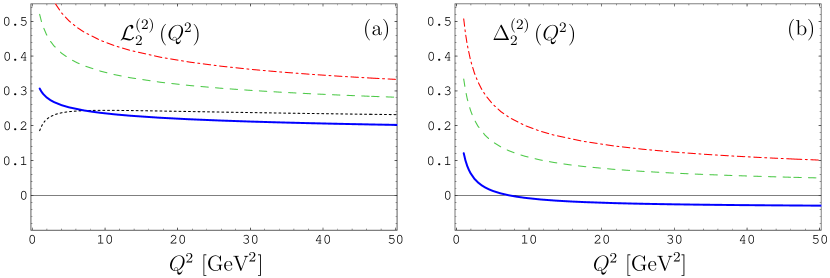
Figure 1: (a): Results for the analyticized logarithmic term, ${\cal L}_{2}^{(2)}\left(Q^{2}\right)$, using three different “analytization” procedures: the one-loop approximate KS “analytization”, ${\cal L}_{2}^{(1)\,\text{approx}}\left(Q^{2}\right)$ (red dash-dotted line), the two-loop approximate KS “analytization”, ${\cal L}_{2}^{(2)\,\text{approx}}\left(Q^{2}\right)$ (green dashed line), and the exact two-loop BMKS “analytization” ${\cal L}_{2}^{(2)}\left(Q^{2}\right)$ (blue solid line). For comparison, we also show here the corresponding maximal “analytization” curve (dotted line). (b): Results are shown for the corresponding analyticized contributions $\Delta_{2}^{(2)}\left(Q^{2}\right)$, using the same three “analytization” procedures for ${\cal L}_{2}^{(2)}\left(Q^{2}\right)$ as in panel (a).

Second, we discuss an analogous situation, in which the one-loop coupling in the denominator is (inconsistently) traded for its two-loop counterpart. In this case, the ratio of the couplings after “analytization” becomes (dashed line in Fig. 1a)

$${\cal L}_{2}^{(2)\,\text{approx}}\left(Q^{2}\right)=\frac{4\pi}{b_{0}}\,{\cal A}_{1}^{(2)}\left(Q^{2}\right)\,.$$ (28)

Finally, we provide the exact result for the KS “analytization” of expression (26) (solid line in Fig. 1a), with the derivation presented in Appendix C, while more general expressions are given in BMS05 :

$${\cal L}_{2}^{(2)}\left(Q^{2}\right)=\frac{4\pi}{b_{0}}\,\left[{\cal A}_{1}^{(2)}\left(Q^{2}\right)+c_{1}\,\frac{4\pi}{b_{0}}\,f_{\cal L}\left(Q^{2}\right)\right]\,,$$ (29)

where

$$f_{\cal L}\left(Q^{2}\right)=\sum_{n\geq 0}\left[\psi(2)\zeta(-n-1)-\frac{d\zeta(-n-1)}{dn}\right]\,\frac{\left[-\ln\left(Q^{2}/\Lambda^{2}\right)\right]^{n}}{\Gamma(n+1)}$$ (30)

and $\zeta(z)$ is the Riemann zeta-function. Equation (25) is illustrated in Fig. 1b for the different expressions of ${\cal L}_{2}\left(Q^{2}\right)$ given by Eqs. (27), (28), and (29), using the same line designations as in Fig. 1a. Let us close this discussion by commenting that in the region where there are experimental data available FFPI73 ; JLAB00 (i.e., well below 10 GeV²), Eq. (25) is governed by ${\cal L}_{2}^{(2)}\left(Q^{2}\right)$, which entails a small enhancement of the hard-scattering amplitude for $Q^{2}\leq 7.25$ GeV².

IV Factorized Pion Form Factor at NLO—Standard and Analyticized

The calculation of the factorized pion form factor proceeds in terms of Eq. (1) and involves the convolution of expression (21) for the maximal “analytization” case, or expression (24) for the KS “analytization” case with the pion DA for which we employ in both cases the BMS parameterization BMS01 , as discussed in Sec. II. On that basis, we can obtain the scaled, factorized part of the pion form factor, $Q^{2}F_{\pi}^{\text{Fact}}\left(Q^{2};\mu_{\text{R}}^{2}=\lambda_{\text{R}}Q^{2}\right)$, using Eq. (8) and the following set of substitutions:

$$t_{\text{H}}^{(0)}(x,y) \rightarrow 8\,\pi\,f_{\pi}^{2}\,\left(1+a_{2}+a_{4}\right)^{2}\,;$$ (31)

$$-\,t_{\text{H}}^{(0)}(x,y)\,\ln\overline{x}\,\overline{y}\, \rightarrow 8\,\pi\,f_{\pi}^{2}\,\left(1+a_{2}+a_{4}\right)\,\left[3+(43/6)a_{2}+(136/15)a_{4}\right]\,;~{}~{}~{}$$ (32)

$$t_{\text{H}}^{(\text{FG})}(x,y) \rightarrow 8\,\pi\,f_{\pi}^{2}\,\big{[}-15.67-a_{2}\left(21.52-6.22\,a_{2}\right)$$ (33)

$$~{}~{}~{}~{}~{}~{}~{}~{}~{}-a_{4}\left(7.37-37.40\,a_{2}-33.61\,a_{4}\right)\big{]}\,.$$

Notice that evolving the BMS pion DA from the initial scale ${\mu_{0}^{2}}$ to the scale $\mu_{\text{F}}^{2}$ at the NLO level will generate higher Gegenbauer harmonics of the form $x\,\overline{x}\,C^{3/2}_{2n}(2x-1)$ with $n\geq 3$. However, we have shown in BPSS04 (see also BS05 ) that for the calculation of the pion form factor it is actually sufficient to restrict ourselves to the LO evolution and neglect NLO evolution effects. Hence, for our purposes in the present analysis, we set

$$a_{2n}(\mu_{\text{F}}^{2})=a_{2n}({\mu_{0}^{2}})\left[\frac{\alpha_{s}(\mu_{\text{F}}^{2})}{\alpha_{s}({\mu_{0}^{2}})}\right]^{\gamma_{n}^{(0)}/(2b_{0})}\,.$$ (34)

The lowest-order anomalous dimensions can be represented in closed form by

$$\gamma_{n}^{(0)}=2C_{\text{F}}\left[4S_{1}(n+1)-3-\frac{2}{(n+1)(n+2)}\right]$$ (35)

with $S_{1}(n+1)=\sum_{i=1}^{n+1}1/i=\psi(n+2)-\psi(1)$, while the function $\psi(z)$ is defined as $\psi(z)=d\ln\Gamma(z)/dz$.

Following the master plan for “analytization”, exposed in the previous section, we obtain the following expressions for the factorized pion form factor:

• Naive “analytization” BPSS04 ; SSK99 ; SSK00 :

  $$\left[F_{\pi}^{\text{Fact}}(Q^{2};\lambda_{\rm R}Q^{2})\right]_{\text{NaivAn}} = {\cal A}_{1}^{(2)}(\lambda_{\rm R}Q^{2})\,{\cal F}_{\pi}^{\text{LO}}\left(Q^{2}\right)$$ (36)

  $$+ \frac{1}{\pi}\,\left[{\cal A}_{1}^{(2)}(\lambda_{\rm R}Q^{2})\right]^{2}\,{\cal F}_{\pi}^{\text{NLO}}\left(Q^{2},\mu_{\text{F}}^{2};\lambda_{\rm R}\right)\,.$$

• Maximal “analytization” BPSS04 :

  $$\left[F_{\pi}^{\text{Fact}}(Q^{2};\lambda_{\rm R}Q^{2})\right]_{\text{MaxAn}} = {\cal A}_{1}^{(2)}(\lambda_{\rm R}Q^{2})\,{\cal F}_{\pi}^{\text{LO}}\left(Q^{2}\right)$$ (37)

  $$+ \frac{1}{\pi}\,{\cal A}_{2}^{(2)}(\lambda_{\rm R}Q^{2})\,{\cal F}_{\pi}^{\text{NLO}}\left(Q^{2},\mu_{\text{F}}^{2};\lambda_{\rm R}\right)\,.$$

• KS amplitude “analytization” (this work)—cf. Eqs. (24) and (26):

  $$\left[F_{\pi}^{\text{Fact}}(Q^{2};\lambda_{\rm R}Q^{2})\right]_{\text{KS}} = {\cal A}_{1}^{(2)}(\lambda_{\rm R}Q^{2})\,{\cal F}_{\pi}^{\text{LO}}\left(Q^{2}\right)$$ (38)

  $$+ \frac{1}{\pi}\,{\cal A}_{2}^{(2)}(\lambda_{\rm R}Q^{2})\,{\cal F}_{\pi}^{\text{NLO}}\left(Q^{2},\mu_{\text{F}}^{2};\lambda_{\rm R}\right)$$

  $$+ \frac{\Delta_{2}^{(2)}\left(\lambda_{\text{R}}Q^{2}\right)}{\pi}\,\Delta_{\text{F}}{\cal F}_{\pi}^{\text{NLO}}\left(Q^{2}\right)\,.~{}~{}~{}~{}~{}~{}$$

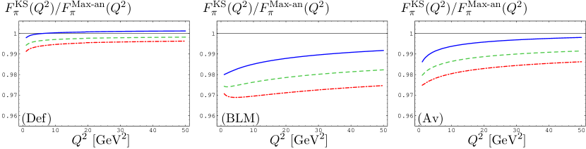
Figure 2: Results for the ratio of the factorized pion form factors, using two different “analytization” procedures: KS “analytization” and “maximal analytization”, $F^{\text{KS}}_{\pi}\left(Q^{2}\right)/F^{\text{Max-an}}_{\pi}\left(Q^{2}\right)$. The designations are: red dash-dotted line—one-loop approximation of the KS logarithmic term (${\cal L}_{2}^{(1)\,\text{approx}}\left(Q^{2}\right)$); green dashed line—two-loop approximation (${\cal L}_{2}^{(2)\,\text{approx}}\left(Q^{2}\right)$); blue solid line—exact two-loop KS “analytization” (${\cal L}_{2}^{(2)}\left(Q^{2}\right)$). Left panel: default scale setting ($\lambda=1$); middle panel: BLM scale setting; right panel: $\alpha_{V}$ scheme. The factorization scale $\mu_{\text{F}}^{2}$ is set equal to $5.76$ GeV² SY99 .

Here we use the following notations:

$${\cal F}_{\pi}^{\text{LO}}\left(Q^{2}\right) = \frac{8\,\pi\,f_{\pi}^{2}}{Q^{2}}\,\left(1+a_{2}+a_{4}\right)^{2}\,;$$ (39)

$$~{}~{}~{}{\cal F}_{\pi}^{\text{NLO}}\left(Q^{2},\mu_{\text{F}}^{2};\lambda_{\rm R}\right) = \frac{2\,\pi\,f_{\pi}^{2}}{Q^{2}}\,\Big{[}b_{0}\left(1+a_{2}+a_{4}\right)^{2}\left(\ln\lambda_{\text{R}}-\ln\lambda_{\text{BLM}}(a_{2},a_{4})\right)-15.67$$ (40)

$$~{}~{}~{}~{}~{}~{}-a_{2}\left(21.52-6.22\,a_{2}\right)-a_{4}\left(7.37-37.40\,a_{2}-33.61\,a_{4}\right)\Big{]}$$

$$+ \Delta_{\text{F}}{\cal F}_{\pi}^{\text{NLO}}\left(Q^{2}\right)\ln\frac{Q^{2}}{\mu_{\text{F}}^{2}}$$

and we explicitly display the contribution due to $t_{\text{H},2}^{(1,\text{F})}\left(x,y;\mu_{\text{F}}^{2}/Q^{2}\right)$, see Eq. (7b):

$$\Delta_{\text{F}}{\cal F}_{\pi}^{\text{NLO}}(Q^{2}) = -\frac{2\,\pi\,f_{\pi}^{2}}{Q^{2}}\,C_{\text{F}}\,\left(1+a_{2}+a_{4}\right)\left[(25/3)a_{2}+(182/15)a_{4}\right]\,.$$ (41)

In order to make our formulas more compact, we implement the BLM scale:

$$\lambda_{\text{BLM}}(a_{2},a_{4})=\exp\left[-\frac{5}{3}-\frac{3+\displaystyle(43/6)a_{2}+(136/15)a_{4}}{1+a_{2}+a_{4}}\right]\,.$$ (42)

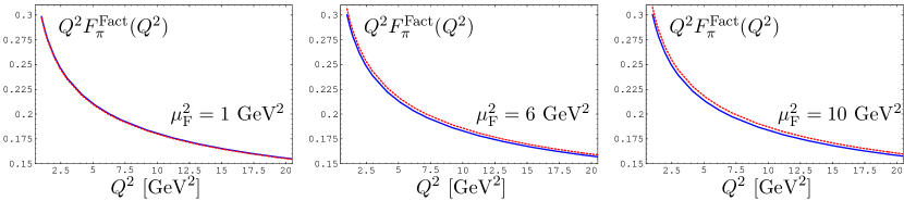
Figure 3: Results for the factorized pion form factors, using two different “analytization” procedures: KS “analytization” (blue solid line) and “maximal analytization” (dotted red line) for different values of the factorization scale: in the left panel $\mu_{\text{F}}^{2}=1$ GeV², in the middle one–$\mu_{\text{F}}^{2}=1$ GeV², and in the right one–$\mu_{\text{F}}^{2}=10$ GeV². For all panels we show results for the BLM scale setting.

The “analytization” augmented perturbation theory works very well. This is illustrated by the results in Figs. 2, 3, and 4. The first of these figures compares the specific issues of the KS “analytization” procedure relative to those of the maximal one for the ratio of the corresponding factorized form factors. A few words are in order here. One sees that using the default $\overline{\text{MS}\vphantom{{}^{1}}}$ scheme, the KS “analytization” procedure yields a result almost coincident with that provided by the maximal one. On the other hand, in the BLM scheme and also in the $\alpha_{V}$ scheme, the KS prediction is smaller by a few percent. Moreover, one observes by comparison with Fig. 11, right panel in Ref. BPSS04 that the BLM prediction, which in the maximal procedure was the largest one, becomes in the case of the KS prescription comparable with the prediction of the default scheme. As a result, the inherent theoretical uncertainties due to the involved perturbative parameters, defining a renormalization scheme and scale setting, are further reduced. A second important feature of the KS procedure is that the dependence of $F_{\pi}^{\rm Fact}(Q^{2})$ on the factorization scale is almost diminished, as indicated in Fig. 3. Indeed, varying the factorization scale from 1 GeV² to 10 GeV², the form factor changes by a mere 1.5 percent. Even setting the factorization scale to the theoretical value of 50 GeV², the induced variation in the form-factor magnitude reaches just the level of about 2.5 percent. In the case of the maximal “analytization” procedure, the dependence on the factorization scale is also a mild one, but the corresponding variation is, in round terms, two times larger.

The fourth figure demonstrates the impact of “analytization” on the factorized pion’s electromagnetic form factor, using various “analytization” prescriptions. The dashed line denotes the prediction obtained with standard QCD perturbation theory in the $\overline{\text{MS}\vphantom{{}^{1}}}$ scheme and applying the default scale setting $\mu_{\rm R}^{2}=Q^{2}$. The naive “analytization” prediction is represented by the dash-dotted line and the analogous one for the maximal “analytization” by the solid line below it. The result of the calculation according to the KS “analytization” practically coincides with that of the maximal one. This behavior is also reflected in Fig. 2, where we see that the differences among the three “analytization” procedures are of the order of a few percent in the whole $Q^{2}$ range considered.

Note that as regards the whole pion form factor, i.e., taking into account also the soft part, the differences would be further reduced. For full details the reader is referred to BPSS04 .

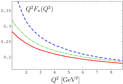
Figure 4: Results for the factorized pion form factor, scaled with $Q^{2}$, and assuming the default scale setting ($\mu_{\text{R}}^{2}=Q^{2}$) in standard perturbation theory and APT. The latter is implemented in terms of two different “analytization” procedures: naive “analytization” and maximal “analytization”. The designations are: blue dashed line—standard perturbation theory; green dash-dotted line—naive APT; red solid line—maximal APT. The prediction obtained with the KS “analytization” is too close to that found with the maximal one to differentiate these curves graphically. The factorization scale $\mu_{\text{F}}^{2}$ is set equal to $5.76$ GeV².

V Summary and Conclusions

We have discussed different “analytization” procedures to ensure the analyticity of the factorized electromagnetic pion form factor at NLO of QCD perturbation theory. The main features and relative merits of each “analytization” concept following from the presented analysis are:

• The naive “analytization SSK99 ; SSK00 retains the power-series expansion of perturbative QCD, but replaces $(\alpha_{s}^{(n)}(Q^{2}))^{m}$ by $({\cal A}_{1}^{(n)}(Q^{2}))^{m}$. As it was shown in SSK99 ; SSK00 , this reduces the value of the NLO correction, though the sensitivity to the renormalization scheme adopted and the renormalization scale-setting chosen is still substantial, resulting into a rather strong variation of the form-factor predictions BPSS04 . Moreover, this procedure does not respect nonlinear relations of the coupling because these correspond to different dispersive images.

• The maximal “analytization” BPSS04 trades the power-series expansion for a functional non-power-series expansion in terms of ${\cal A}_{m}^{(n)}(Q^{2})$ SS97 ; Shi00 ; SS01 , minimizing the variation of the form-factor predictions owing to the renormalization scheme and scale setting. It is, however, insufficient to cure logarithms of the momentum scale multiplying the running coupling. Such terms modify the spectral density, i.e., the discontinuity across the cut along the negative real axis and have therefore to be taken into account.

• Applying the “analytization” procedure at the level of the partonic amplitude itself KS01 ; Ste02 , bears all advantages of the maximal “analytization” plus a further reduced dependence on the perturbative scales—especially the dependence on the factorization scale. This has been verified by explicit calculation. We have employed the $\overline{\text{MS}\vphantom{{}^{1}}}$ scheme with various scale settings and also the $\alpha_{V}$ scheme. In addition, we have varied the factorization scale in the range $1-10$ GeV². While the predictions for the factorized pion form factor, calculated with the maximal procedure, were affected by this variation on the level of 3%, their counterparts, derived with the KS prescription, were influenced by less than 1%. Though the KS method does not really “gain up” relative to the maximal “analytization” procedure with respect to the factorized pion form factor, as one observes from Fig. 4, it is able to further improve the perturbative treatment because it extends the notion of analyticity to non-integer powers of the strong running coupling—FAPT. Such powers become relevant when one has to calculate the analytic image of powers of the strong coupling in combination with logarithms, the latter first appearing at NLO of fixed-order perturbation theory, or in terms of evolution factors BMS05 . Hence, the KS “analytization” requirement treats all logarithms that have a non-zero spectral density, and hence modify the discontinuity across the cut along the negative real axis, on the same footing and irrespective of their source being it the running coupling (and its powers), or logarithms entailed by ERBL or DGLAP evolution.

In conclusion, the KS “analytization” enables the variation of the factorization scale and the choice of various renormalization schemes and scale settings, including the BLM one, with undiminished quality of the theoretical predictions from scheme (scale) to scheme (scale), virtually eliminating the dependence on such parameters and upgrading the $\overline{\text{MS}\vphantom{{}^{1}}}$ scheme to an optimized factorization and renormalization scheme. From a broader perspective one may interpret these findings as indicating that the analyticity of the partonic three-point function is as important and fundamental as the underlying symmetries of the theory and should be preserved together with them in the maximal possible way.

Appendix A QCD $\beta$ function at NLO

The first coefficients of the $\beta$ function are

$$b_{0}=\frac{11}{3}\,C_{\text{A}}-\frac{4}{3}\,T_{\text{R}}N_{f}\,,\qquad\qquad b_{1}=\frac{34}{3}\,C_{\text{A}}^{2}-\left(4C_{\text{F}}+\frac{20}{3}\,C_{\text{A}}\right)T_{\text{R}}N_{f}\,.$$ (43)

Here, $T_{\text{R}}=1/2$ and $N_{f}$ denotes the number of flavors, whereas the expansion of the $\beta$-function in the NLO approximation is given by

$$\beta(\alpha_{s}(\mu^{2}))=-\alpha_{s}(\mu^{2})\left[b_{0}\left(\frac{\alpha_{s}(\mu^{2})}{4\pi}\right)+b_{1}\left(\frac{\alpha_{s}(\mu^{2})}{4\pi}\right)^{2}\right]\,.$$ (44)

Appendix B NLO correction to the pion form factor

Here we present the detailed expressions for the color decomposition of the NLO correction to the hard amplitude $T_{\text{H}}$, which describe the factorized part of the pion form factor MNP98 ; BPSS04 (see Eqs. (5)–(7b)):

$$t_{\text{H},1}^{(1,\text{F})}(x,y) = \frac{N_{\text{T}}}{\overline{x}\,\overline{y}\,}\left[-\frac{28}{3}+\left(6-\frac{1}{x}\right)\ln\overline{x}\,+\left(6-\frac{1}{y}\right)\ln\overline{y}\,+\ln^{2}(\overline{x}\,\overline{y}\,)\right]\,;$$ (45)

$$t_{\text{H}}^{(1,\text{G})}(x,y) = \frac{2N_{\text{T}}}{\overline{x}\,\overline{y}\,}\left[-\frac{10}{3}+\ln\left(\frac{\overline{x}\,}{x}\right)\ln\left(\frac{y}{\overline{y}\,}\right)-4\left(\frac{\ln\overline{x}\,}{x}+\frac{\ln\overline{y}\,}{y}\right)\!-\!\tilde{H}(x,y)-R(x,y)\right].~{}~{}~{}~{}~{}~{}$$ (46)

The functions $\tilde{H}(x,y)$ and $R(x,y)$ are defined by

$$\tilde{H}(x,y)=\left[{\textbf{Li}_{2}}\left(\frac{\overline{y}\,}{x}\right)+{\textbf{Li}_{2}}\left(\frac{\overline{x}\,}{y}\right)+{\textbf{Li}_{2}}\left(\frac{xy}{\overline{x}\,\overline{y}\,}\right)-{\textbf{Li}_{2}}\left(\frac{x}{\overline{y}\,}\right)-{\textbf{Li}_{2}}\left(\frac{y}{\overline{x}\,}\right)-{\textbf{Li}_{2}}\left(\frac{\overline{x}\,\overline{y}\,}{xy}\right)\right]~{}~{}~{}~{}$$ (47)

and

$$R(x,y)\!\!\!\!\! =\!\frac{1}{(x-y)^{2}}\Bigl{[}(2xy-x-y)(\ln x+\ln y)-(y\overline{y}\,^{2}+x\overline{x}\,^{2})(1-x-y)\tilde{H}(x,\overline{y}\,)$$ (48)

$$-2\left(xy^{2}+y^{2}-5xy+y+2x^{2}\right)\frac{\ln\overline{y}\,}{y}-2\left(yx^{2}+x^{2}-5xy+x+2y^{2}\right)\frac{\ln\overline{x}\,}{x}\Bigr{]}.$$

Appendix C “Analytization” of powers of the coupling multiplied by logarithms

We present here the derivation of ${\cal L}_{2}^{(2)}\left(Q^{2}\right)$, done in collaboration with S. Mikhailov. To this end, let us first introduce

$$a_{s}\left(Q^{2}\right)\equiv\frac{b_{0}}{4\pi}\,\alpha_{s}\left(Q^{2}\right)\,.$$ (49)

For this quantity we can write a renormalization group solution in the form

$$\left[a_{s}^{(2)}\left(Q^{2}\right)\right]^{2}\ln\left(\frac{Q^{2}}{\Lambda^{2}}\right)=a_{s}^{(2)}\left(Q^{2}\right)+\left[a_{s}^{(2)}\left(Q^{2}\right)\right]^{2}\,c_{1}\,\ln\left[\frac{a_{s}^{(2)}\left(Q^{2}\right)}{1+c_{1}a_{s}^{(2)}\left(Q^{2}\right)}\right]\,.$$ (50)

Expanding the expression $\ln[1+c_{1}a_{s}^{(2)}\left(Q^{2}\right)]$ and retaining terms up to order $a_{s}^{2}$, we find

$$\left[a_{s}^{(2)}\left(Q^{2}\right)\right]^{2}\ln\left(\frac{Q^{2}}{\Lambda^{2}}\right)=a_{s}^{(2)}\left(Q^{2}\right)+\left[a_{s}^{(2)}\left(Q^{2}\right)\right]^{2}\,c_{1}\,\ln\left[a_{s}^{(2)}\left(Q^{2}\right)\right]\,.$$ (51)

To get rid of the logarithm, we use the following trick

$$\left[a_{s}^{(2)}\left(Q^{2}\right)\right]^{2}\ln\left(\frac{Q^{2}}{\Lambda^{2}}\right)=a_{s}^{(2)}\left(Q^{2}\right)+c_{1}\,\frac{d}{d\varepsilon}\left[a_{s}^{(2)}\left(Q^{2}\right)\right]^{2+\varepsilon}\Big{|}_{\varepsilon=0}$$ (52)

and return to the original coupling to obtain

$$\left[\alpha_{s}^{(2)}\left(Q^{2}\right)\right]^{2}\ln\left(\frac{Q^{2}}{\Lambda^{2}}\right)=\frac{4\pi}{b_{0}}\,\alpha_{s}^{(2)}\left(Q^{2}\right)+c_{1}\,\frac{4\pi}{b_{0}}\,\frac{d}{d\varepsilon}\left[\alpha_{s}^{(2)}\left(Q^{2}\right)\right]^{2+\varepsilon}\Big{|}_{\varepsilon=0}\,.$$ (53)

Now we can proceed with the “analytization ” of the term $[\alpha_{s}^{(2)}\left(Q^{2}\right)]^{2}\ln\left(Q^{2}\right)$, giving rise to analytic expressions for non-integer powers of the coupling, i.e.,

$$\left\{\left[\alpha_{s}^{(2)}\left(Q^{2}\right)\right]^{2}\ln\left(\frac{Q^{2}}{\Lambda^{2}}\right)\right\}_{\text{an}}=\frac{4\pi}{b_{0}}\,{\cal A}_{1}^{(2)}\left(Q^{2}\right)+c_{1}\left[\frac{d}{d\varepsilon}\,{\cal A}_{2+\varepsilon}^{(2)}\left(Q^{2}\right)\right]_{\varepsilon=0}\,.$$ (54)

Using the representation BMS05

$$\left(\frac{b_{0}}{4\pi}\right)^{2}{\cal A}_{\nu}^{(2)}\left(Q^{2}\right)=\frac{-1}{\Gamma(\nu)}\,\sum_{n\geq 0}\zeta(1-\nu-n)\frac{\left[-\ln\left(Q^{2}/\Lambda^{2}\right)\right]^{n}}{\Gamma(n+1)}$$ (55)

and performing the differentiation, we finally obtain

$$\left\{\left[\alpha_{s}^{(2)}\left(Q^{2}\right)\right]^{2}\ln\left(\frac{Q^{2}}{\Lambda^{2}}\right)\right\}_{\text{an}}=\frac{4\pi}{b_{0}}\,\left[{\cal A}_{1}^{(2)}\left(Q^{2}\right)+c_{1}\,\frac{4\pi}{b_{0}}\,f_{\cal L}\left(Q^{2}\right)\right]\,,$$ (56)

with $f_{\cal L}\left(Q^{2}\right)$ being defined in Eq. (30).

References

• (1) J. M. Cornwall, Phys. Rev. D 26 (1982) 1453.
• (2) G. Parisi, R. Petronzio, Nucl. Phys. B 154 (1979) 427.
• (3) C. R. Ji, A. F. Sill, R. M. Lombard-Nelsen, Phys. Rev. D 36 (1987) 165.
• (4) N. G. Stefanis, Phys. Rev. D 40 (1989) 2305; Phys. Rev. D 44 (1991) 1616, Erratum.
• (5) C. R. Ji, F. Amiri, Phys. Rev. D 42 (1990) 3764.
• (6) N. G. Stefanis, M. Bergmann, Phys. Lett. B 304 (1993) 24.
• (7) A. C. Mattingly, P. M. Stevenson, Phys. Rev. D 49 (1994) 437.
• (8) S. J. Brodsky, C. R. Ji, A. Pang, D. G. Robertson, Phys. Rev. D 57 (1998) 245.
• (9) D. Müller, Phys. Rev. D 59 (1999) 116003.
• (10) N. G. Stefanis, Eur. Phys. J. direct C 7 (1999) 1, hep-ph/9911375.
• (11) D. V. Shirkov, I. L. Solovtsov, Phys. Rev. Lett. 79 (1997) 1209.
• (12) D. V. Shirkov, Theor. Math. Phys. 119 (1999) 438, Teor. Mat. Fiz. 119 (1999) 55, hep-th/9810246.
• (13) I. L. Solovtsov, D. V. Shirkov, Theor. Math. Phys. 120 (1999) 1220, Teor. Mat. Fiz. 120 (1999) 482, hep-ph/9909305.
• (14) D. V. Shirkov, hep-ph/0003242; hep-ph/0009106; hep-ph/0408272.
• (15) I. L. Solovtsov, D. V. Shirkov, Phys. Lett. B 442 (1998) 344.
• (16) D. V. Shirkov, Theor. Math. Phys. 127 (2001) 409, hep-ph/0012283; Eur. Phys. J. C 22 (2001) 331.
• (17) D. V. Shirkov, I. L. Solovtsov, Phys. Part. Nucl. 32S1 (2001) 48.
• (18) D. S. Kourashev, B. A. Magradze, hep-ph/0104142; Theor. Math. Phys. 135 (2003) 531, Teor. Mat. Fiz. 135 (2003) 95.
• (19) B. A. Magradze, Int. J. Mod. Phys. A 15 (2000) 2715, hep-ph/9911456; hep-ph/0010070; hep-ph/0305020.
• (20) S. J. Brodsky, S. Menke, C. Merino, J. Rathsman, Phys. Rev. D 67 (2003) 055008.
• (21) A. I. Alekseev, hep-ph/0503242.
• (22) A. V. Radyushkin, JINR Rapid Commun. 78 (1996) 96, hep-ph/9907228.
• (23) N. V. Krasnikov, A. A. Pivovarov, Phys. Lett. B 116 (1982) 168.
• (24) M. Beneke, V. M. Braun, Phys. Lett. B 348 (1995) 513.
• (25) P. Ball, M. Beneke, V. M. Braun, Nucl. Phys. B 452 (1995) 563.
• (26) K. A. Milton, I. L. Solovtsov, Phys. Rev. D 55 (1997) 5295;
K. A. Milton, I. L. Solovtsov, O. P. Solovtsova, Phys. Lett. B 415 (1997) 104.
• (27) A. P. Bakulev, A. V. Radyushkin, N. G. Stefanis, Phys. Rev. D 62 (2000) 113001.
• (28) A. V. Nesterenko, Int. J. Mod. Phys. A 18 (2003) 5475; hep-ph/0308288.
• (29) A. V. Nesterenko, J. Papavassiliou, Phys. Rev. D 71 (2005) 016009; hep-ph/0410072;
A. C. Aguilar, A. V. Nesterenko, J. Papavassiliou, hep-ph/0504195.
• (30) N. G. Stefanis, W. Schroers, H. C. Kim, Phys. Lett. B 449 (1999) 299.
• (31) N. G. Stefanis, W. Schroers, H. C. Kim, Eur. Phys. J. C 18 (2000) 137.
• (32) A. I. Karanikas, N. G. Stefanis, Phys. Lett. B 504 (2001) 225.
• (33) N. G. Stefanis, Lect. Notes Phys. 616 (2003) 153, hep-ph/0203103; Invited talk at 11th International Conference in Quantum ChromoDynamics (QCD 04), Montpellier, France, 5-9 Jul 2004, to be published in Nucl. Phys. Proc. Suppl., hep-ph/0410245.
• (34) S. J. Brodsky, H. J. Lu, Phys. Rev. D 51 (1995) 3652.
• (35) A. P. Bakulev, K. Passek-Kumerički, W. Schroers, N. G. Stefanis, Phys. Rev. D 70 (2004) 033014; Phys. Rev. D 70 (2004) 079906 Erratum;
N. G. Stefanis, A.P. Bakulev, S. V. Mikhailov, K. Passek-Kumerički, W. Schroers, Invited talk at Workshop on Hadron Structure and QCD: From Low to High Energies (HSQCD 2004), St. Petersburg, Repino, Russia, 18-22 May 2004, to be published in the Proceedings, hep-ph/0409176.
• (36) A. P. Bakulev, S. V. Mikhailov, N. G. Stefanis, Phys. Rev. D72 (2005) 074014.
• (37) A. V. Efremov, A. V. Radyushkin, Phys. Lett. B 94 (1980) 245; Theor. Math. Phys. 42 (1980) 97.
• (38) G. P. Lepage, S. J. Brodsky, Phys. Rev. D 22 (1980) 2157.
• (39) B. Melić, B. Nižić, K. Passek, Phys. Rev. D 60 (1999) 074004; Phys. Rev. D 65 (2002) 053020.
• (40) S. J. Brodsky, G. P. Lepage, P. B. Mackenzie, Phys. Rev. D 28 (1983) 228.
• (41) A. P. Bakulev, S. V. Mikhailov, N. G. Stefanis, Phys. Lett. B 508 (2001) 279; Phys. Lett. B 590 (2004) 309 Erratum; in: Proceedings of the 36th Rencontres De Moriond On QCD And Hadronic Interactions, 17-24 Mar 2001, Les Arcs, France, edited by J. T. T. Van (World Scientific, Singapour, 2002), p. 133, hep-ph/0104290.
• (42) A.P. Bakulev, S.V. Mikhailov, N.G. Stefanis, Phys. Rev. D 67 (2003) 074012.
• (43) A. P. Bakulev, S. V. Mikhailov, N. G. Stefanis, Phys. Lett. B 578 (2004) 91; Phys. Part. Nucl. 35 (2004) 7, hep-ph/0312141.
• (44) CLEO Collaboration, J. Gronberg et al., Phys. Rev. D 57 (1998) 33.
• (45) A. P. Bakulev, S. V. Mikhailov, N. G. Stefanis, Ann. Phys. (Leipzig) 13 (2004) 629, hep-ph/0410138.
• (46) CELLO Collaboration, H.J. Behrend et al., Z. Phys. C 49 (1991) 401.
• (47) Y. L. Dokshitzer, G. Marchesini, B. R. Webber, Nucl. Phys. B 469 (1996) 93.
• (48) H. Contopanagos, G. Sterman, Nucl. Phys. B 419 (1994) 77.
• (49) S. Catani, M. L. Mangano, P. Nason, L. Trentadue, Nucl. Phys. B 478 (1996) 273.
• (50) L. Magnea, Nucl. Phys. B 593 (2001) 269.
• (51) E. Gardi, Nucl. Phys. B 622 (2002) 365.
• (52) R. Alkofer, L. von Smekal, Phys. Rept. 353 (2001) 281.
• (53) M. Baldicchi, G. M. Prosperi, in International Conference On Color Confinement And Hadrons In Quantum Chromodynamics – Confinement 2003, 21–24 Jul 2003, Wako, Japan, edited by H. Suganuma et al. (World Scientific, Singapore, 2004), pp. 183–194 [hep-ph/0310213]; AIP Conf. Proc. 756, 152 (2005), invited talk given at the 6th Conference on Quark Confinement and the Hadron Spectrum, Villasimius, Sardinia, Italy, 21–25 Sep 2004 [hep-ph/0412359].
• (54) The Jefferson Lab F(pi) Collaboration, J. Volmer et al., Phys. Rev. Lett. 86 (2001) 1713; H. P. Blok, G. M. Huber, D. J. Mack, nucl-ex/0208011.
• (55) C. N. Brown et al., Phys. Rev. D 8 (1973) 92; C. J. Bebek et al., Phys. Rev. D 13 (1976) 25.
• (56) A. P. Bakulev, N. G. Stefanis, Nucl. Phys. B 721 (2005) 50.
• (57) A. Schmedding, O. Yakovlev, Phys. Rev. D 62 (2000) 116002.