UNIFICATION WITHOUT SUPERSYMMETRY:
NEUTRINO MASS, PROTON DECAY AND LIGHT LEPTOQUARKS

Abstract

We investigate predictions of a minimal realistic non-supersymmetric $SU(5)$ grand unified theory. To accomplish unification and generate neutrino mass we introduce one extra Higgs representation—a $\bm{15}$ of $SU(5)$—to the particle content of the minimal Georgi-Glashow scenario. Generic prediction of this setup is a set of rather light scalar leptoquarks. In the case of the most natural implementation of the type II see-saw mechanism their mass is in the phenomenologically interesting region ($O(10^{2}$–$10^{3})$ GeV). As such, our scenario has a potential to be tested at the next generation of collider experiments, particularly at the Large Hadron Collider (LHC) at CERN. The presence of the $\bm{15}$ generates additional contributions to proton decay which, for light scalar leptoquarks, can be more important than the usual gauge $d=6$ ones. We exhaustively study both and show that the scenario is not excluded by current experimental bounds on nucleon lifetimes.

I Introduction

The most predictive grand unified theory (GUT) based on an $SU(5)$ gauge symmetry is a minimal non-supersymmetric model of Georgi and Glashow GG (GG). However, the failure to accommodate experimentally observed fermion masses and mixing and to unify electroweak and strong forces decisively rule it out. Nevertheless, the main features of the underlying theory, e.g, partial matter unification and one-step symmetry breaking, are so appealing that there has been a number of proposals to enlarge its structure by adding more representations to have the theory in agreement with experimental data. Since the number of possible extensions is large it is important to answer the following question. What is the minimal number of extra particles that renders an $SU(5)$ gauge theory realistic? Such an extension of the GG model with the smallest possible number of extra particles that furnish full $SU(5)$ representation(s) has all prerequisites to be the most predictive one. Thus, if there is a definite answer to the first question it is important to ask the second one: What are the possible experimental signatures and associated uncertainties of such a minimal setup? If uncertainties of the minimal extension are significant the same is even more true of a more complicated structure unless additional assumptions are imposed. We address both questions in great detail and present truly minimal, i.e., minimal in terms of number of fields, realistic non-supersymmetric $SU(5)$ scenario.

As we demonstrate later, unification, in the minimal scenario, points towards existence of light scalar leptoquarks which could generate very rich phenomenological signatures. These are looked for in the direct search experiments as well as in the experiments looking for rare processes. Their presence generates novel proton decay contributions which can be very important. Moreover, since in our scheme their coupling to matter is through the Majorana neutrino Yukawas, their observation might even allow measurements of and/or provide constraints on neutrino Yukawa coupling entries. This makes our scenario extremely attractive. At the same time, rather low scale of vector leptoquarks that is inherent in non-supersymmetric theories exposes our scenario to the tests via nucleon lifetime measurements. We investigate all relevant experimental signatures of the scenario, including its status with respect to the present bounds on nucleon lifetime.

In the next section we define our framework. In Section III we discuss how it is possible to get gauge couplings unification in agreement with low energy data. Then, in Section IV we discuss possible experimental signatures of the minimal scenario. We conclude in Section V. Appendix A contains relevant details and notation of the minimal non-supersymmetric realistic $SU(5)$ we refer to throughout the manuscript. The origin of theoretical bounds on the familiar gauge $d=6$ proton decay operators is critically analyzed in Appendix B. Appendix C contains details on the two-loop running of the gauge couplings that is presented for completeness of our work.

II A minimal realistic non-supersymmetric $SU(5)$ scenario

In order to motivate the minimal $SU(5)$ grand unifying theory (GUT), where we define such a theory to be the one with the smallest possible particle content that renders it realistic, we first revisit the GG model GG and discuss its shortcomings. Only then do we present the minimal realistic scenario and investigate its experimental signatures and related uncertainties.

The GG model fails from the phenomenological point of view for a number of reasons:

1. It does not incorporate massive neutrinos;

2. It yields charged fermion mass ratios in gross violation of experimentally observed values;

3. It cannot account for the gauge coupling unification. (For one of the first rulings on (non)unification see for example Ref. Marciano .)

The first flaw is easy to fix; one either introduces three right-handed neutrinos—singlets of the Standard Model (SM)—to use a type I see-saw mechanism seesaw to generate their mass or adds a Higgs field—a $\bm{15}$ of $SU(5)$—to generate neutrino mass through the so-called type II see-saw Lazarides ; Mohapatra . One might also use the combination of the two. The fourth option to use the Planck mass suppressed higher-dimensional operators Weinberg ; Barbieri does not look promising since it generates too small scale for neutrino mass to explain the atmospheric and solar neutrino data. Nevertheless, it might still play an important role GoranBerezhiani . We focus our attention on the second option, i.e., addition of $\bm{15}$, in view of the fact that the right-handed neutrinos, being singlets of the SM, do not contribute to the running. Hence, their mass scale cannot be sufficiently well determined or constrained unless additional assumptions are introduced.

The second flaw can be fixed by either introducing the higher-dimensional operators in the Yukawa sector Ellis:1 or resorting to a more complicated Higgs sector à la Georgi and Jarlskog GJ . The former approach introduces a lot more parameters into the model (see for example Bajc2 ) but unlike in the neutrino case these operators might have just a right strength to modify “bad” mass predictions for the charged fermions. In order to keep as minimal as possible the number of particles we opt for the scenario with the non-renormalizable terms.

The third flaw requires presence of additional non-trivial split representations besides those of the GG $SU(5)$ model. It can thus be fixed in conjunction with the first and second one. For example, introduction of an extra $\bm{45}$ of Higgs to fix mass ratios of charged fermions à la Georgi and Jarlskog GJ allows one to achieve unification and, at the same time, raise the scale relevant for proton decay. (For the studies on the influence of an extra $\bm{45}$ on the running and other predictions see for example BabuMa ; Giveon .) We will see that the addition of one extra $\bm{15}$ of Higgs plays a crucial role in achieving the unification in our case.

So, what we have in mind as the minimal realistic $SU(5)$ model is the GG model supplemented by the $\bm{15}$ of Higgs to generate neutrino mass and which incorporates non-renormalizable effects to fix the Yukawa sector of charged fermions. We analyze exclusively non-supersymmetric scenario for the following three reasons: first, this guarantees the minimality of the number of fields; second, there are no problems with the $d=4$ and $d=5$ proton decay operators; third, since the grand unifying scale is lower than in supersymmetric scenario the setup could possibly be verified or excluded in the next generation of proton decay experiments.

III Unification of gauge couplings

The main prediction, besides the proton decay, of any GUT is the unification of the strong and electroweak forces. We thus show that it is possible to achieve gauge coupling unification in a consistent way in our scenario.

At the one-loop level the running of gauge couplings is given by

$$\alpha^{-1}_{i}|_{M_{Z}}=\alpha^{-1}_{GUT}+\frac{1}{2\pi}b_{i}\ln\frac{M_{GUT}}{M_{Z}},$$ (1)

where $i=1,2,3$ for $U(1)$, $SU(2)$, and $SU(3)$, respectively. $b_{i}$ are the appropriate one-loop coefficients Cheng and $\alpha_{GUT}=g^{2}_{GUT}/(4\pi)$ represents the gauge coupling at the unifying scale $M_{GUT}$. The SM coefficients for the case of $n$ light Higgs doublet fields are:

$$b_{1}=\frac{40}{10}+\frac{n}{10},\qquad\qquad b_{2}=-\frac{20}{6}+\frac{n}{6},\qquad\qquad b_{3}=-7.$$ (2)

Even though the SM coefficients do not generate unification in both the $n=1$ and $n=2$ case for any value of $\alpha_{GUT}$ and $M_{GUT}$ that is not an issue since the SM does not predict the gauge coupling unification in the first place. On the other hand, a GUT, which does predict one, automatically introduces a number of additional particles with respect to the SM case that, if light enough, can change the outcome of the SM running. This change is easily incorporated if one replaces $b_{i}$ in Eq. (1) with the effective one-loop coefficients $B_{i}$ defined by

$$B_{i}=b_{i}+\sum_{I}b_{iI}r_{I},\qquad r_{I}=\frac{\ln M_{GUT}/M_{I}}{\ln M_{GUT}/M_{Z}},$$ (3)

where $b_{iI}$ are the one-loop coefficients of any additional particle $I$ of mass $M_{I}$ ($M_{Z}\leq M_{I}\leq M_{GUT}$). Basically, given a particle content of the GUT and Eqs. (1) and (3) we can investigate if the unification is possible.

Following Giveon et al Giveon , Eqs. (1) can be further rewritten in a more suitable form in terms of differences in the effective coefficients $B_{ij}(=B_{i}-B_{j})$ and low energy observables. They find two relations that hold at $M_{Z}$:

$$\frac{B_{23}}{B_{12}} = \frac{5}{8}\frac{\sin^{2}\theta_{w}-\alpha_{em}/\alpha_{s}}{3/8-\sin^{2}\theta_{w}},$$ (4a)

$$\ln\frac{M_{GUT}}{M_{Z}} = \frac{16\pi}{5\alpha_{em}}\frac{3/8-\sin^{2}\theta_{w}}{B_{12}}.$$ (4b)

Adopting the following experimental values at $M_{Z}$ in the $\overline{MS}$ scheme PDG2004 : $\sin^{2}\theta_{w}=0.23120\pm 0.00015$, $\alpha_{em}^{-1}=127.906\pm 0.019$ and $\alpha_{s}=0.1187\pm 0.002$, we obtain

$$\frac{B_{23}}{B_{12}} = 0.719\pm 0.005,$$ (5a)

$$\ln\frac{M_{GUT}}{M_{Z}} = \frac{184.9\pm 0.2}{B_{12}}.$$ (5b)

Last two equations allow us to constrain the mass spectrum of additional particles that leads to an exact unification at $M_{GUT}$. (In what follows we consistently use central values presented in Eqs. (5) unless specified otherwise. The inclusion of the two-loop effects and threshold corrections is addressed in detail in Appendix C.)

The fact that the SM with one (two) Higgs doublet(s) cannot yield unification is now more transparent in light of Eq. (5a). Namely, the resulting SM ratio is simply too small ($B_{23}/B_{12}=0.53$ for $n=1$) to satisfy equality in Eq. (5a). What is needed is one or more particles that are relatively light and with suitable $b_{i}$ coefficients that can increase the value of the $B_{23}/B_{12}$ ratio. The most efficient enhancement is realized by a field that increases $B_{23}$ and decreases $B_{12}$ simultaneously. For example, light Higgs doublet is such a field (see the $\Psi_{D}(\subset\bm{5}_{H})$ coefficients in Table 1) and it takes at least eight of them, at the one-loop level, to bring $B_{23}/B_{12}$ in accord with experiments. Other fields that could generate the same type of improvement in our scenario are light $\Sigma_{3}(\subset\bm{24}_{H})$, $\Phi_{a}(\subset\bm{15}_{H})$ and $\Phi_{b}(\subset\bm{15}_{H})$. $B_{ij}$ coefficients of all the particles in our scenario are presented in Table 1 and the relevant notation is set in Appendix A.

Table 1: Contributions to the $B_{ij}$coefficients. The mass of the SM Higgs doublet is taken to be at $M_{Z}$.

	Higgsless SM	$\Psi_{D}$	$\Psi_{T}$	$V$	$\Sigma_{8}$	$\Sigma_{3}$	$\Phi_{a}$	$\Phi_{b}$	$\Phi_{c}$
$B_{23}$	$\frac{11}{3}$	$\frac{1}{6}$	$-\frac{1}{6}r_{\Psi_{T}}$	$-\frac{7}{2}r_{V}$	$-\frac{1}{2}r_{\Sigma_{8}}$	$\frac{1}{3}r_{\Sigma_{3}}$	$\frac{2}{3}r_{\Phi_{a}}$	$\frac{1}{6}r_{\Phi_{b}}$	$-\frac{5}{6}r_{\Phi_{c}}$
$B_{12}$	$\frac{22}{3}$	$-\frac{1}{15}$	$\frac{1}{15}r_{\Psi_{T}}$	$-7r_{V}$	0	$-\frac{1}{3}r_{\Sigma_{3}}$	$-\frac{1}{15}r_{\Phi_{a}}$	$-\frac{7}{15}r_{\Phi_{b}}$	$\frac{8}{15}r_{\Phi_{c}}$

The improvement can also be due to the field that lowers $B_{12}$ only or lowers $B_{12}$ at sufficiently faster rate than $B_{23}$. Looking at Table 1 we see that the superheavy gauge fields $V$ comprising $X$ and $Y$ gauge bosons and their conjugate partners can accomplish the latter. (Note that the gauge contribution improves unification at the one-loop level only if $n\neq 0$ and the improvement grows with the increase of $n$ Giveon ; MY . This is because the $B_{23}/B_{12}$ ratio of the Higgsless SM coefficients is the same as for the corresponding ratio of $V$ coefficients.) But, their contribution to running has to be subdominant; otherwise one runs into conflict with the experimental data on nucleon lifetimes.

All in all, the fields capable of improving unification in our minimal $SU(5)$ grand unified scenario are $\Psi_{D}$, $\Sigma_{3}$, $\Phi_{a}$, $\Phi_{b}$ and $V$. Again, we refer reader to Appendix A for our notation. We treat their masses as free parameters and investigate the possibility for consistent scenario with the exact one-loop unification. Since all other fields in the Higgs sector, i.e., $\Psi_{T}$, $\Sigma_{8}$ and $\Phi_{c}$, simply worsen unification we simply assume they live at or above the grandunifying scale.

In order to present consistent analysis we now discuss the constraints coming from proton decay on $B_{ij}$ coefficients. These enter via Eq. (5b) and assumption that $M_{V}=M_{GUT}$. As we show these constraints are rather weak if the gauge $d=6$ contributions are dominant as is usually assumed in non-supersymmetric GUTs Buras . For example, if we use the latest bounds on nucleon decay lifetimes we obtain, in the context of an $SU(5)$ non-supersymmetric GUT, in the case of maximal (minimal) suppression in the Yukawa sector Ilja3 $M_{V}>2.5\times 10^{13}$ GeV ($M_{V}>1.5\times 10^{15}$ GeV). (The minimal suppression case corresponds to the GG scenario with $Y_{U}=Y^{T}_{U}$ and $Y_{D}=Y^{T}_{E}$, where $Y_{U}$, $Y_{D}$ and $Y_{E}$ are the Yukawa matrices of charged fermions. Non-renormalizable contributions violate both of those relations. The same is also true for the running in the Yukawa sector from the GUT scale where those relations hold to the scale relevant for the Yukawa couplings entering nucleon decay. On the other hand, maximal suppression corresponds to a case with particular relation between unitary matrices responsible for bi-unitary transformations in the Yukawa sector Ilja3 that define physical basis for quarks and leptons.) In both cases we use $\alpha^{-1}_{GUT}=35$ and the best limit on partial lifetime which is established for $p\rightarrow\pi^{0}e^{+}$ decay channel ($\tau>5.0\times 10^{33}$ years). This gives conservative bound for the suppressed case since it is always possible to rotate away proton decay contributions for individual channels Ilja3 .

The uncertainty in extracting the limits on $M_{V}$ from experimental data is easy to understand. Namely, even though the nucleon lifetime is proportional to $M_{V}^{4}$, which would make extraction rather accurate and precise, the lifetime is also proportional to the fourth power of a term which is basically a sum of entries of unitary matrices which are a priori unknown unless the Yukawa sector of the GUT theory is specified and which, in magnitude (see Eqs. (25)), can basically vary from $V_{ub}$ to $1$ Nandi ; Ilja3 . (For full discussion see also Appendix B.) If we now adopt the $M_{GUT}\equiv M_{V}$ assumption and use Eq. (5b) the above limits translate into $B_{12}<7.0$ ($B_{12}<6.1$) for the suppressed (unsuppressed) case. So, all $SU(5)$ GUTs with $B_{12}>7.0$ are excluded by the usual gauge $d=6$ contributions to proton decay. The theories with $6.1<B_{12}<7.0$ require “special” structure of the Yukawa sector; the closer the $B_{12}$ to the upper limit is the more “special” structure is needed. Finally, any $SU(5)$ GUT with $B_{12}<6.1$ has not yet been probed by proton decay experiments. (Again, this is all based on the one-loop analysis. Any more accurate and precise statement must be based on the two-loop treatment with a proper inclusion of the threshold corrections.)

In order to avoid problems with proton decay without requiring too much conspiracy in the Yukawa sector we pursue the solutions where the superheavy gauge bosons are as heavy as possible. So, how heavy can they be given the particle content of the $SU(5)$ scenario with an extra $\bm{15}$ of Higgs? In order to answer that we first naively set masses of $\Sigma_{3}$, $\Phi_{a}$ and $\Phi_{b}$ to $M_{Z}$. This in turn yields the lowest possible value of $B_{12}$ to be $6.4$ ($6.33$) for $n=1$ ($n=2$) which translates via Eq. (5b) into $M_{GUT}=3.2\times 10^{14}$ GeV ($M_{GUT}=4.4\times 10^{14}$ GeV). (We include $n=2$ case in our considerations since it might be relevant in addressing Baryon asymmetry of the Universe.) In this naive estimate $M_{V}$ is either equal to or slightly above $M_{GUT}$. From the previous discussion on the $M_{V}$ limits we see that there is a need for small suppression in Yukawa sector in order to satisfy experimental limits on proton decay. This suppression, as we show later, amounts to a $1/5$ of the unsuppressed case. When compared to the available suppression ($\sim 1/V_{ub}$) it comes out to be around $2\%$, which can easily be accomplished.

Note, however, that in order to have exact unification crucial thing is to satisfy Eq. (5a). Thus, it is better to ask for which mass spectrum that satisfies Eq. (5a) we obtain the highest possible value for $M_{V}$ or equivalently the smallest possible value for $B_{12}$. As it turns out the answer to this question is unique within our scenario. To show that we first assume that the relevant degrees of freedom that improve the running, i.e., $\Sigma_{3}$, $\Phi_{a}$ and $\Phi_{b}$, contribute in pairs, e.g., a degenerate pair $(\Sigma_{3},\Phi_{a})$ is light and $\Phi_{b}$ is at $M_{GUT}$, and treat only the $n=2$ case. With those constraints we generate three possible combinations which yield results summarized in Table 2. (We address both the $n=1$ and $n=2$ case at the two-loop level in Appendix C.)

Table 2: $\Delta B_{23}$ and $\Delta B_{12}$ corrections due to the degenerate pairs of fields and the associated scales for the $n=2$ case.

	$(\Sigma_{3},\Phi_{a})$	$(\Sigma_{3},\Phi_{b})$	$(\Phi_{a},\Phi_{b})$
$\Delta B_{23}$	$\frac{6}{6}r+\frac{2}{6}$	$\frac{3}{6}r+\frac{2}{6}$	$\frac{5}{6}r+\frac{2}{6}$
$\Delta B_{12}$	$-\frac{6}{15}r-\frac{2}{15}$	$-\frac{12}{15}r-\frac{2}{15}$	$-\frac{8}{15}r-\frac{2}{15}$
$M_{GUT}$	$5\times 10^{13}$ GeV	—	$9\times 10^{13}$ GeV
$M_{r}$	$1$ TeV	—	$200$ GeV

• The $(\Sigma_{3},\Phi_{a})$ case with $n=2$ exactly mimics the $n=8$ case in terms of quantum numbers. (Recall that it takes at least eight light Higgs doublets on top of the Higssless SM content to unify the couplings. Associated corrections to the Higssless SM coefficients are $\Delta B_{23}=\frac{6}{6}r+\frac{2}{6}$ and $\Delta B_{12}=-\frac{6}{15}r-\frac{2}{15}$, where $r$, as defined in Eq. (3), is very close to one and we take two of the doublets to be at $M_{Z}$.) The unification scale is rather low and very close to the experimentally set limit for maximally suppressed case. Lightness of $\Phi_{a}$ goes against the idea behind the type II see-saw if one assumes that the parameter $c_{3}$ (see Eqs. (17) and (23)) is at the GUT scale, but at this point the scenario is not ruled out experimentally.

• The $(\Phi_{a},\Phi_{b})$ case has a slightly higher unification scale than the $(\Sigma_{3},\Phi_{a})$ case. This time both $\Phi_{a}$ and $\Phi_{b}$ have mass in phenomenologically interesting region. Lightness of $\Phi_{a}$ again requires large suppression in the Yukawa sector for neutrinos to generate correct mass scale via type II see-saw. However, such a suppression would be beneficial in suppressing novel contributions to proton decay due to the mixing between $\Phi_{b}$ and $\Psi_{T}$.

• The $(\Sigma_{3},\Phi_{b})$ case is the most promising. Even though it fails to unify at the one-loop level its correction to $B_{12}$ is the largest of all three cases. As such, it represents the best possible candidate to maximize $M_{V}$. Moreover, the $\Phi_{a}$ contribution to the running to produce unification for light $\Sigma_{3}$ and $\Phi_{b}$ is small which implies that its mass could be in the range that is optimal for the type II see-saw for the most “natural” value of $c_{3}$ coefficient. Again, the $(\Sigma_{3},\Phi_{b})$ case not only maximizes $M_{V}$ but also places $M_{\Phi_{a}}$ at the right scale to explain neutrino masses.

The three special cases discussed above all demonstrate that large $M_{V}$ scale prefers $\Phi_{b}$ light regardless of the relevant scale of other particles since it is $\Phi_{b}$ coefficients that decrease $B_{12}$ the most. These conclusions persist in more detailed one- and two-loop studies.

Is there a way to tell between the three limiting cases we just discussed? The $(\Sigma_{3},\Phi_{a})$ case can be tested and excluded by slight improvement in the nucleon lifetime data; other low energy signatures depend on how light $\Phi_{a}$ is. One could also test and distinguish between the $(\Sigma_{3},\Phi_{b})$ and $(\Phi_{a},\Phi_{b})$ cases since both favor light $\Phi_{b}$ leptoquarks that can be detected by LHC. If and when these are detected the two cases could be distinguished by the scalar leptoquark contributions to the rare processes. In the $(\Phi_{a},\Phi_{b})$ case the suppression in the neutrino Yukawa sector would selectively erase some of these contribution while in the $(\Sigma_{3},\Phi_{b})$ case all these contributions would be sizable. Expected improvements in the table-top experiments would then be sufficient to tell the two.

Since we have $M_{GUT}$ and masses of $V$, $\Sigma_{3}$, $\Phi_{a}$ and $\Phi_{b}$ as free parameters and only two equations—Eqs. (5a) and (5b)—we present four special cases based on certain simplifying assumptions in Figs. 1, 2 and 3 and discuss each case in turn. All examples we present generate consistent unification in agreement with low energy data. (Note that the change in the parameters also affects the value of $\alpha^{-1}_{GUT}$. We do not present that change explicitly, which, for the range of values we use, vary from $36$ to $40$. In our plots we also allow $M_{V}$ to be at most factor of three or four lower than the GUT scale. Once we switch to two-loop analysis with threshold corrections accounted for we appropriately set $M_{V}=M_{GUT}$.)

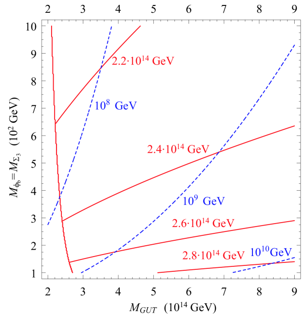
Figure 1: Plot of lines of constant value of $M_{V}$ (solid lines) and $M_{\Phi_{a}}$ (dashed lines) in the $M_{GUT}$–$(M_{\Sigma_{3}}=M_{\Phi_{b}})$ plane. The area to the left of a steep solid line denotes the region where $M_{V}$ does not contribute to the running, i.e., $M_{V}\geq M_{GUT}$. To generate the plot we consider exact one-loop unification and use central values for the gauge couplings as given in the text. This is a scenario with one light Higgs doublet ($n=1$).

In Fig. 1 we present the $n=1$ case when the pair ($\Sigma_{3}$,$\Phi_{b}$) is taken to be degenerate with the mass close to electroweak scale ($\sim O(10^{2})$ GeV). The parameter $c_{3}$ has to be between $10^{3}$ and $10^{7}$ GeV to explain the neutrino mass through the type II see-saw if the Yukawa coupling for neutrinos is of order one. On the other hand, the gauge boson mass varies only slightly for a given range of $M_{\Phi_{b}}$ and $M_{\Sigma_{3}}$ around $2.5\times 10^{14}$ GeV. Clearly, unification itself allows $M_{\Phi_{b}}$ and $M_{\Sigma_{3}}$ to be much heavier then 1 TeV on account of decrease of $M_{\Phi_{a}}$ but in that case $M_{V}$ would be getting lighter. This, on the other hand would require additional conspiracy in the Yukawa sector in order to sufficiently suppress proton decay to avoid the experimental limit.

The two light Higgs doublet case is presented in Fig. 2. This case is well motivated on the Baryogenesis grounds. Namely, the interaction of the $\bm{15}$ of Higgs explicitly breaks $B-L$ symmetry (see Appendix A). This opens a door for possible explanation of the Baryon asymmetry in the Universe within our framework. However, since the successful generation of Baryon asymmetry requires at least two Higgses in the fundamental representation we study a consistent unification picture for that case. (See references for the Baryogenesis mechanisms in the context of $SU(5)$ model with two Higgses in the fundamental representation Barr ; Nanopoulos ; Yildiz ; Fukugita ). The $n=2$ case has higher scale of superheavy gauge bosons compared to the $n=1$ case (this does not hold at the two-loop level though) and the mass of the field $\Phi_{a}$ is in the region relevant for the type II see-saw. Hence, if the mass of scalar leptoquarks is in phenomenologically interesting region ($\sim O(10^{2})$ GeV) we can explain neutrino masses naturally. Again, as in the $n=1$ case, the gauge boson mass varies very slightly, this time around $3\times 10^{14}$ GeV.

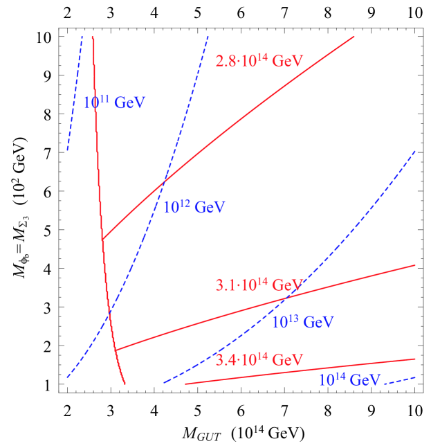
Figure 2: Plot of lines of constant value of $M_{V}$ (solid lines) and $M_{\Phi_{a}}$ (dashed lines) in the $M_{GUT}$–$(M_{\Sigma_{3}}=M_{\Phi_{b}})$ plane. The area to the left of a steep solid line denotes the region where $M_{V}$ does not contribute to the running, i.e., $M_{V}\geq M_{GUT}$. This is the $n=2$ scenario.

Given the last two examples we can again conclude that the exact unification in this minimal realistic scenario points towards light scalar leptoquarks.

In order to understand better these results we show two more examples in Fig. 3. This time we set $\Sigma_{3}=\Phi_{a}$ for simplicity and present both $n=1$ and $n=2$ cases. This scenario is disfavored by the fact that $M_{V}$ tends to be “small” but cannot be excluded on experimental grounds. It is evident from the plot that $M_{V}$ does not depend on a number of light Higgs doublets and $M_{GUT}$. The reason for that is very simple and is valid only at the one-loop level. Namely, the ratio $B_{23}/B_{12}$ is the same for $\Psi_{D}$ coefficients ($=-5/2$) as for the sum of corresponding $\Sigma_{3}$ and $\Phi_{a}$ coefficients provided these are degenerate. Thus, any change in the number of light doublets in Eq. (5a) is simply compensated by the change in degenerate mass of $\Sigma_{3}$ and $\Phi_{a}$ fields for a fixed value of $\Phi_{b}$ mass. This trend can be clearly seen in Fig. 3. The mass of $\Phi_{a}$ is generally rather low to generate neutrino mass of correct magnitude unless Yukawa couplings of neutrinos are extremely small.

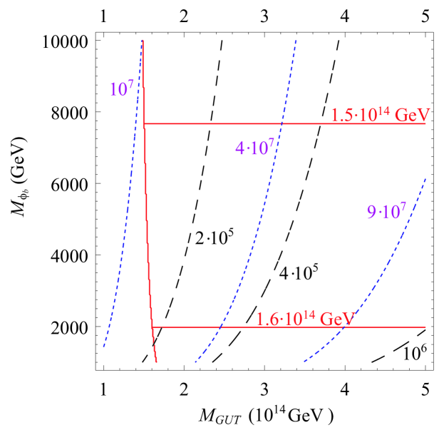
Figure 3: Plot of lines of constant value of $M_{V}$ (solid lines) and $M_{\Phi_{a}}=M_{\Sigma_{3}}$ in GeV units (dashed lines) in the $M_{GUT}$–$(M_{\Phi_{b}})$ plane. The scenario with one (two) Higgs doublet(s) corresponds to long (short) dashed lines.

In all our examples, $\Sigma_{3}$ is allowed to be much lighter than $\Sigma_{8}$. But, this seems in conflict with the tree-level analysis of the $\Sigma$ potential that is invariant under $\Sigma\rightarrow-\Sigma$ transformation which yields a well known relation $M_{\Sigma_{3}}=4M_{\Sigma_{8}}$ Buras . This apparent mismatch has a simple remedy.

In order to generate sufficiently large corrections to charged fermion masses via higher-dimensional operators in the Yukawa sector we need terms linear in $\Sigma/M_{Pl}$. If that is the case it is no longer possible to require that the Lagrangian is invariant under transformation $\Sigma\rightarrow-\Sigma$. It is then necessary to include a cubic term into the $\Sigma$ potential besides the usual quadratic and quartic ones. But, the potential with the cubic term ($Tr\Sigma^{3}$) violates the validity of $M_{\Sigma_{3}}=4M_{\Sigma_{8}}$ relation Li ; Guth:1 ; Guth:2 and allows a possibility where $\Sigma_{3}$ is light while $\Sigma_{8}$ is superheavy. We analyze this situation in Appendix A in some detail. Note that we do not require nor insist on the lightness of $\Sigma_{3}$ though. In Appendix C we present the two-loop analysis of the scenario where $\Phi_{a}$ is relatively light ($\sim 10^{7}$ GeV) and $\Sigma_{3}$ is at the GUT scale. Our intention is solely to demonstrate that there are more possibilities available unless additional assumptions, such as $\Sigma\rightarrow-\Sigma$ transformation, are imposed on the $SU(5)$ theory. Note, however, that the maximization of $M_{V}$ always requires $\Phi_{b}$ to be very light ($\sim 10^{2}$ GeV). In Fig. 4 we show an example where it is possible to achieve unification at the two-loop level (See details in Appendix C) for $n=1$, $M_{\Phi_{b}}=250$ GeV, $M_{\Phi_{a}}=1.54$ TeV and the field $\Sigma_{3}$ is at the GUT scale.

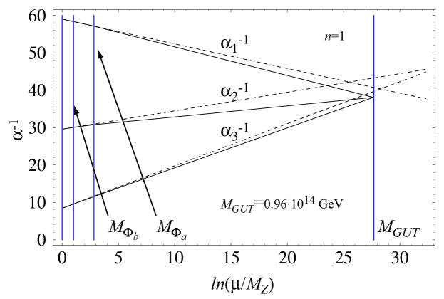
Figure 4: Unification of the gauge couplings at the two-loop level for central values of low-energy observables PDG2004 . The SM case with $n=1$ is presented by dashed lines. Solid lines correspond to the $n=1$ scenario with $\Phi_{b}$ and $\Phi_{a}$ below the GUT scale. Vertical lines mark the relevant scales: $M_{Z}$, $M_{\Phi_{b}}=250$ GeV, $M_{\Phi_{a}}=1.54$ TeV and $M_{GUT}=0.96\times 10^{14}$ GeV.

What about the possible mass spectrum of $\Phi_{a}$, $\Phi_{b}$ and $\Phi_{c}$? The relevant potential is in Appendix A. Clearly, there are more parameters than mass eigenvalues. The tree-level analysis revels that it is possible to obtain any possible arrangement including, for example, $\Phi_{b}\ <<\ \Phi_{a}\ <\ \Phi_{c}$. This sort of split is quite similar to the split behind the well-known Doublet-Triplet problem.

Our framework yields rather low mass for vector leptoquarks that varies within very narrow range around $3\times 10^{14}$ GeV for a most plausible scenarios. This makes the framework testable through nucleon decay measurements. (More precisely, large portion of the parameter space of the setup has already been excluded by existing measurements on nucleon lifetime.) It is easy to understand this generic and robust prediction. We have seen that $M_{GUT}$ can be at most $3.2\times 10^{14}$ GeV ($4.4\times 10^{14}$ GeV) if we exclude the $V$ contribution from the running for the $n=1$ ($n=2$) case. If we now start lowering $M_{V}$ below $M_{GUT}$ we lower $B_{12}$ as well. This, on the other hand, starts to increase $M_{GUT}$ but still keeps $M_{V}$ at almost the same value. Basically, the “decoupling” of $M_{V}$ and $M_{GUT}$ takes place, where the mass of $X$ and $Y$ gauge bosons remains in vicinity of the value before the “decoupling” while $M_{GUT}$ rapidly approaches the Planck scale. Another way to say this is that the $B_{ij}$ coefficients of superheavy gauge fields are very large compared to all other relevant coefficients (see Table 1). Thus, any small change in $M_{V}$ corresponds to a large change in other running parameters.

Let us finally investigate possible experimental signatures coming from our consistent minimal realistic $SU(5)$ model.

IV Experimental Signatures

Our framework has potential to be tested through the detection—direct or indirect—of light leptoquarks and/or observation of proton decay. Let us investigate each of these tests in turn.

• Light leptoquarks

  To get consistent unification in agreement with low energy data, neutrino mass and proton decay in our minimal framework we generate very light leptoquarks $\Phi_{b}$. The lighter the $\Phi_{b}$ is the heavier the $V$ becomes. Thus, in the most optimistic scenario $M_{\Phi_{b}}$ is close to the present experimental limit $\sim O(10^{2})$ GeV. In what follows we specify all relevant properties of $\Phi_{b}$ and existing constraints on its couplings and mass.

  The $\bar{\bm{5}}_{a}^{T}Ch_{ab}\Phi\bar{\bm{5}}_{b}$ coupling yields the following interactions:

  $${d^{C}}^{T}Ch\Phi_{b}l={d^{C}}^{T}Ch(\phi_{b}^{1}e-\phi_{b}^{2}\nu),$$ (6)

  where the leptoquarks $\phi_{b}^{1}$ and $\phi_{b}^{2}$ have electric charges $2/3$ and $-1/3$, respectively, and symmetric matrix $h$ coincides with the Yukawa coupling matrix of Majorana neutrinos ($\equiv Y_{\nu}$) if we neglect the Planck suppressed operators. (See the last line in Eq. (16).) The above leptoquark interactions in the physical basis read as:

  $${d^{C}}^{T}\ C\ (D_{C}^{T}E^{*})K^{*}(V_{PMNS}^{M})^{*}Y_{\nu}^{\textrm{diag}}(V_{PMNS}^{M})^{\dagger}K^{*}\ \phi_{b}^{1}\ e,$$ (7)

  $${d^{C}}^{T}\ C\ (D_{C}^{T}E^{*})K^{*}(V_{PMNS}^{M})^{*}Y_{\nu}^{\textrm{diag}}\ \phi_{b}^{2}\ \nu,$$ (8)

  where $D_{C}$ and $E$ are the matrices which act on $d^{C}$ quarks and $e$, respectively, to bring them into physical basis. (See Appendix B for exact convention.) $K$ is a matrix containing three CP violating phases, and $V_{PMNS}^{M}$ is the leptonic mixing in the Majorana case. (In the GG $SU(5)$ where $Y_{E}=Y_{D}^{T}$ one has $D_{C}=E$. However, that is not the case in a realistic model for fermion masses.)

  There are many studies about the contributions of scalar and vector leptoquarks in different processes Buchmuller ; Davidson . For a model independent constraints on leptoquarks from rare processes see for example Davidson ; Herz . The most stringent bound on the scalar leptoquark coupling to matter comes from the limits on $\mu$–$e$ conversion on nuclei Dohmen . The bound we present should be multiplied by $(M_{\Phi_{b}}/100\,\textrm{GeV})^{2}$. In our case it reads $(D_{C}^{T}hE)_{11}(E^{\dagger}h^{\dagger}D_{C}^{*})_{21}<10^{-6}$. The bounds for all other elements of $(D_{C}^{T}hE)_{ij}(E^{\dagger}h^{\dagger}D_{C}^{*})_{kl}$ and $(D_{C}^{T}hN)_{ij}(N^{*}h^{\dagger}D_{C}^{*})_{kl}$ are weaker.

  The currents bounds on leptoquarks production are set by Tevatron, LEP and HERA bounds . Tevatron experiments have set limits on scalars leptoquarks with couplings to $eq$ of $M_{LQ}>242$ GeV. The LEP and HERA experiments have set limits which are model dependent. The search for these novel particles will be continued soon at the CERN LHC. Preliminary studies by the LHC experiments ATLAS ATLAS and CMS CMS indicate that clear signals can be established for masses up to about $M_{LQ}\approx 1.3$ TeV. For several studies about production of scalar leptoquarks at the LHC, see Ref. production . Thus, it could be possible to test our scenario at the next generation of colliders, particularly in the Large Hadron Collider (LHC) at CERN, through the production of light leptoquarks. Therefore even without the proton decay experiments we could have tests of this non-supersymmetric GUT scenario.

• Proton decay

  Proton decay is the most generic prediction coming from matter unification; therefore, it is the most promising test for any grand unified theory. (For new experimental bounds see PDG2004 ; newbounds .) In our minimal and consistent scenario the relevant scale for gauge bosons is around $3\times 10^{14}$ GeV regardless of how high the GUT scale goes in order to get consistent unification in agreement with low energy data. Careful study within the two-loop context with the inclusion of threshold effects revels that the highest possible value of $M_{V}$ in the $n=2$ ($n=1$) case is $3.19\times 10^{14}$ GeV ($3.28\times 10^{14}$ GeV) for central values of coupling constants PDG2004 while the $1\,\sigma$ departure allows for the maximum value of $3.35\times 10^{14}$ GeV in the $n=2$ case, for example.

  There are several contributions to the decay of the proton in our minimal scenario. We have the usual Higgs and gauge $d=6$ operators but there are also new contributions due to the mixing between $\Psi_{T}$ and $\Phi_{b}$, with $\Phi_{b}$ being extremely light in our case. These contributions are very important. Using the relevant triplet interactions:

  $$q_{a}\ C\ \underline{A}^{ab}\ q_{b}\ \Psi_{T}\ +\ q_{a}\ C\ \underline{C}^{ab}\ l_{b}\ \Psi_{T}^{*}\ +\ u^{C}_{a}\ C\ \underline{D}^{ab}\ d_{b}^{C}\ \Psi_{T}^{*}\ +\ u^{C}_{a}\ C\ \underline{B}^{ab}\ e_{b}^{C}\ \Psi_{T},$$ (9)

  (for the expressions of $\underline{A}$, $\underline{B}$, $\underline{C}$, and $\underline{D}$ matrices see for example Bajc2 ) and the interaction term $\bar{\bm{5}}_{a}^{T}Ch_{ab}\Phi\bar{\bm{5}}_{b}$, it is easy to write down the contributions for the $B-L$ non-conserving decays $p\to(K^{+},\pi^{+},\rho^{+})\nu_{i}$, and $n\to(\pi^{0},\rho^{0},\eta^{0},w^{0},K^{0})\nu_{i}$. We present the relevant diagram in Fig. 5 Mohapatrabook .

  

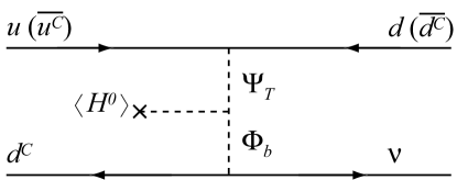
  Figure 5: Contributions to the decay of the proton induced by the $\bm{15}$ of Higgs.

  Notice that in this scenario we have the usual $B-L$ conserving decays, i.e., the decays into a meson and antileptons, and the $B-L$ non-conserving decays mentioned above. Since $\Phi_{b}$ has to be light, the $B-L$ violating decays are very important. The rate for the decays into neutrinos is given by:

  $$\Gamma(p\to K^{+}{\nu}) = \sum_{i=1}^{3}\Gamma(p\to K^{+}{\nu}_{i})=\frac{(m_{p}^{2}-m_{K}^{2})^{2}}{32\pi m_{P}^{3}f_{\pi}^{2}}A_{L}^{2}\frac{c_{3}^{2}<H^{0}>^{2}}{M_{\Psi_{T}}^{4}M_{\Phi_{b}}^{4}}\times$$ (10)

  $$|\tilde{\beta}\ C(\nu_{i},s,d^{C})\ +\ \tilde{\alpha}\ C(\nu_{i},s^{C},d^{C})|^{2}\ \frac{4m_{p}^{2}D^{2}}{9m_{B}^{2}}$$

  $$+ |\tilde{\beta}\ C(\nu_{i},d,s^{C})\ +\ \tilde{\alpha}\ C(\nu_{i},d^{C},s^{C})|^{2}\ [1+\frac{m_{p}(D+3F)}{3m_{B}}]^{2}$$

  where $C(\nu_{i},d_{\alpha},d_{\beta}^{C})=(U^{T}\ (\underline{A}+\underline{A}^{T})D)_{1\alpha}$ and $C(\nu_{i},d_{\alpha}^{C},d_{\beta}^{C})=(D_{C}^{\dagger}\underline{D}^{\dagger}U_{C}^{*})_{\alpha 1}$. (See Appendix B for notation.)

  As you can appreciate from the above expressions, the predictions coming from these contributions are quite model dependent. Using $m_{p}=938.3$ MeV, $D=0.81$, $F=0.44$, $m_{B}=1150$ MeV, $f_{\pi}=139$ MeV, $A_{L}=1.43$, and $\tilde{\alpha}=\tilde{\beta}=\alpha=0.003$ GeV³ we get:

  $$1.95\times 10^{-64}\ \text{GeV}^{-6}\ \frac{M_{\Psi_{T}}^{4}M_{\Phi_{b}}^{4}}{c_{3}^{2}}\ >\ [\ 0.19\ |C(\nu_{i},s,d^{C})\ +\ C(\nu_{i},s^{C},d^{C})|^{2}\ +$$

  $$+\ 2.49\ |C(\nu_{i},d,s^{C})\ +\ C(\nu_{i},d^{C},s^{C})|^{2}\ ]$$ (11)

  Let us see an example, using the values $M_{\Psi_{T}}=c_{3}=10^{14}$ GeV and $M_{\Phi_{b}}=10^{3}$ GeV, the left-hand side of the above equation is equal to $1.95\times 10^{-24}$; therefore, the sum of the $C$ coefficients has to be basically $10^{-12}$. In the case that coefficient $c_{3}$ is smaller ($\sim 10^{6}$ GeV), a possibility that is not excluded, the sum of $C$ coefficients would be around $10^{-4}$, which is their “natural” value. Moreover, the scenario would then prefer $\Phi_{a}$ at the same scale ($\sim 10^{6}$ GeV) if $Y_{\nu}$ is taken to be proportional to $Y_{e}$. Also we can suppress the relevant contributions in different ways. For example, we could choose $\underline{A}_{ij}=-\underline{A}_{ji}$ and $\underline{D}_{ij}=0$ except for $i=j=3$, or set to zero these coefficients in specific models for fermion masses.

  In any case, if the gauge $d=6$ contributions are the dominant ones for proton decay, we can get the following bounds for the proton lifetime (see Appendix B) allowing the full freedom in the Yukawa sector:

  $$1\times 10^{31}\,\text{years}<\tau_{p}<2\times 10^{38}\,\text{years}.$$ (12)

  Here we use $\alpha_{GUT}^{-1}=39$ and $M_{GUT}=3.2\times 10^{14}$ GeV. (See Fig. 6 for example.) Having in mind the experimental limit of $5.0\times 10^{33}$ years PDG2004 we see that a significant portion of available parameter space has already been excluded. We hope that in the next generation of proton decay experiments this scenario would be constrained even further.

How does this scenario compare to other possible extensions of the GG model? We mention only few listing them by increasing order in particle number.

• The most obvious extension is to add one more fundamental representation in the Higgs sector to the $n=2$ scenario we analyze the most at the one-loop level. This addition would not raise but actually lower $M_{V}$ since the scalar leptoquarks which influence $B_{12}$ the most would get slightly heavier than in the $n=2$ case. In certain way, this actually makes the $n=1$ scenario with the $\bm{15}$ of Higgs very unique. It is the minimal extension of the GG model with the highest available scale for $M_{V}$. We focus our attention on the $n=2$ case on the grounds of Baryogenesis. In the same manner, the $n=3$ scenario would be well motivated by the possibility of addressing the issue of the SM model CP violation Branco0 (see also Branco and references therein).

• Very interesting possibility would be the $n=1$ case with two $\bm{10}$s of Higgs. Such a scenario could have a very high GUT scale and still very promising phenomenological consequences due to light leptoquarks. For example, successful two-loop unification with light $\Phi_{b}$s (there are two now) at 250 GeV requires $M_{\Sigma_{3}}=2.1\times 10^{11}$ GeV and the GUT scale at $1.0\times 10^{15}$ GeV for central values of $\alpha_{i}$s at $M_{Z}$. This model would also require at least right-handed neutrinos and non-renormalizable operators to be completely realistic.

• Another possibility would be the $n=1$ case with one $\bm{10}$ and one $\bm{15}$ of Higgs. Such a scenario would have a same maximal value for the GUT scale as the two $\bm{10}$ case above. To be completely realistic it would require non-renormalizable operators.

• The next scenario is the one proposed by Murayama and Yanagida MY (MY). They shown that addition of two $\bm{10}$s of Higgs to the GG model and with $n=2$ it is possible to achieve unification for extremely light scalar leptoquarks in the $\bm{10}$s. This allows MY to forward a “desert” hypothesis, within which the particles are either light ($\sim O(10^{2})$ GeV) or heavy ($\sim O(10^{14})$ GeV). (Note that the scalar leptoquarks with exactly the same quantum numbers as $\Phi_{b}$ ($\subset\bm{15}$) reside in the $\bm{10}$ as well. To see that one can use $\bm{5}\otimes\bm{5}=\bm{10}\oplus\bm{15}$. Note that the couplings of $\Phi_{b}$ in the $\bm{10}$ ($\bm{15}$) to the $\bm{5}$s are antisymmetric (symmetric).) Their model is ruled out by direct searches for scalar leptoquarks due to the extreme lightness of $\Phi_{b}$s. However, if one allows for splitting between $\Sigma_{3}$ and $\Sigma_{8}$ one can raise unification scale sufficiently to avoid proton decay bounds and resurrect their model although one would have to abandon the “desert” hypothesis MY forwarded. The additional contribution to the Higgsless SM coefficient in this case is basically $\Delta B_{12}=-\frac{14}{15}r_{\Phi_{b}}-\frac{5}{15}r_{\Sigma_{3}}-\frac{2}{15}$ which is much more than any of the cases considered in Table 2. For example, for $M_{\Phi_{b}}=300$ GeV we find, at the one-loop level, $M_{\Sigma_{3}}=10^{10}$ GeV and $M_{GUT}=9\times 10^{14}$ GeV. Note that the presence of the $\bm{10}$ of Higgs yields the same type of coupling as we specify in Eq. (6) except that $h$, in this case, would be antisymmetric. This, however, would not a priori prevent proton decay. If there are two or more Higgses in the fundamental representation in the model there exist the proton decay process schematically represented in Fig. 4 unless additional symmetry is introduced. Finally, this model would also require at least right-handed neutrinos and non-renormalizable operators to be completely realistic.

• The Georgi-Jarlskog model GJ with an extra $\bm{45}$ of Higgs to fix fermion masses represents natural extension of the GG model. However, even though unification takes place BabuMa ; Giveon and the extension has good motivation the predictivity of the model is lost unless additional assumptions are introduced. More minimal extension than that would be, for example, an extra $\bm{24}$ of Higgs to the scenario we consider.

V Summary

We have investigated the possibility to get a consistent unification picture in agreement with low energy data, neutrino mass and proton decay in the context of the minimal realistic non-supersymmetric $SU(5)$ scenario. This scenario is the Georgi-Glashow model extended by an extra $\bm{15}$ of Higgs. As generic predictions from the running of the gauge couplings we have that a set of scalar leptoquarks is light, with their mass, in the most optimistic case, being around $O(10^{2}$–$10^{3})$ GeV. This makes possible the tests of this scenario at the next generation of collider experiments, particularly in the Large Hadron Collider (LHC) at CERN. In the “least” optimistic scenario the mass of the scalar leptoquarks would be around $10^{5}$ GeV. The proton decay issue has been studied in detail, showing that it is possible to satisfy all experimental bounds with very small, at $2\%$ level, suppression in Yukawa sector. Rather low scale of vector leptoquarks ($\sim 3\times 10^{14}$ GeV) already allows for significant exclusion of available parameter space of our scenario. Further reduction is expected in near future with new limits on proton decay lifetime. We have particularly studied the case with two Higgses in the fundamental representation since in this case it could be possible to explain the Baryon asymmetry of the Universe. We have also compared this scenario with other, well motivated, extensions of the GG model. There are uncertainties related to predictions of the proposed scenario but, in view of the fact that it truly represents the minimal realistic extension of the GG model, the same is even more true of all other extensions.

Appendix A Particle Content And Relevant Interactions

In this appendix we define a minimal realistic non-supersymmetric $SU(5)$ model. By minimal we refer to the minimal number of physical fields such a model requires. In the GG model the matter is unified in two representations: $\bar{\bm{5}}_{a}=(d^{C},l)_{a}$, and $\bm{10}_{a}=(u^{C},q,e^{C})_{a}$, where $a=1,2,3$ is a generation index. The Higgs sector comprises $\mathbf{{5}}_{H}=\Psi=(\Psi_{D},\Psi_{T})$ and $\mathbf{24}_{H}=\Sigma=(\Sigma_{8},\Sigma_{3},\Sigma_{(3,2)},\Sigma_{(\bar{3},2)},\Sigma_{24})$. However, this model does not achieve unification and fails to correctly accommodate fermion masses; therefore, it is ruled out. In the introduction we discuss how it is possible to solve all phenomenological problems of the GG model introducing a minimal set of fields. Namely, it is sufficient to introduce an extra representation: $\mathbf{15}_{H}=\Phi=(\Phi_{a},\Phi_{b},\Phi_{c})$. The SM decomposition of the Higgs sector is given by:

$$\bm{24}_{H} = \Sigma=(\bm{8},\bm{1},0)+(\bm{1},\bm{3},0)+(\bm{3},\bm{2},-5/6)+(\overline{\bm{3}},\bm{2},5/6)+(\bm{1},\bm{1},0),$$ (13)

$$\bm{15}_{H} = \Phi=(\bm{1},\bm{3},1)+(\bm{3},\bm{2},1/6)+(\bm{6},\bm{1},-2/3),$$ (14)

$$\bm{5}_{H} = \Psi=(\bm{1},\bm{2},1/2)+(\bm{3},\bm{1},-1/3).$$ (15)

The relevant Yukawa potential, up to order $1/M_{Pl}$, is

$$V_{\textrm{Yukawa}} = \epsilon_{ijklm}\left(\bm{10}_{a}^{ij}f_{ab}\bm{10}_{b}^{kl}\Psi^{m}+\bm{10}_{a}^{ij}f_{1ab}\bm{10}_{b}^{kl}\frac{\Sigma^{m}_{~{}n}}{M_{Pl}}\Psi^{n}+\bm{10}_{a}^{ij}f_{2ab}\bm{10}_{b}^{kn}\Psi^{l}\frac{\Sigma^{m}_{~{}n}}{M_{Pl}}\right)$$ (16)

$$+ \Psi^{*}_{i}\bm{10}_{a}^{ij}g_{ab}\bar{\bm{5}}_{bj}+\Psi^{*}_{i}\frac{\Sigma^{i}_{~{}j}}{M_{Pl}}\bm{10}_{a}^{jk}g_{1ab}\bar{\bm{5}}_{bk}+\Psi^{*}_{i}\bm{10}_{a}^{ij}g_{2ab}\frac{\Sigma_{~{}j}^{k}}{M_{Pl}}\bar{\bm{5}}_{bk}$$

$$+ \Phi^{ij}\bar{\bm{5}}_{ai}h_{ab}\bar{\bm{5}}_{bj}+\frac{(\bar{\bm{5}}_{ai}\Psi^{i})h_{1ab}(\bar{\bm{5}}_{bj}\Psi^{j})}{M_{Pl}},$$

where $i,j,k,l,m$ represent $SU(5)$ indices. Impact of the non-renormalizable operators on the fermion masses is discussed in Ellis:1 . Notice that we could replace $M_{Pl}$ by a scale $\Lambda$, where $M_{GUT}\ <\ \Lambda\ <\ M_{Pl}$, if we do not assume a desert between the GUT scale and the Planck scale. (See for example reference Shafi .)

The Higgs scalar potential, manifestly invariant under $SU(5)$, is (see for example Ruegg ; Buccella ):

$$V_{\textrm{Higgs}} = -\frac{\mu_{\Sigma}^{2}}{2}\Sigma^{i}_{~{}j}\Sigma^{j}_{~{}i}+\frac{a_{\Sigma}}{4}(\Sigma^{i}_{~{}j}\Sigma^{j}_{~{}i})^{2}+\frac{b_{\Sigma}}{2}\Sigma^{i}_{~{}j}\Sigma^{j}_{~{}k}\Sigma^{k}_{~{}l}\Sigma^{l}_{~{}i}+\frac{c_{\Sigma}}{3}\Sigma^{i}_{~{}j}\Sigma^{j}_{~{}k}\Sigma^{k}_{~{}i}$$ (17)

$$- \frac{\mu_{\Psi}^{2}}{2}\Psi^{*}_{i}\Psi^{i}+\frac{a_{\Psi}}{4}(\Psi^{*}_{i}\Psi^{i})^{2}-\frac{\mu_{\Phi}^{2}}{2}\Phi_{ij}^{*}\Phi^{ij}+\frac{a_{\Phi}}{4}(\Phi_{ij}^{*}\Phi^{ij})^{2}+\frac{b_{\Phi}}{2}\Phi_{ij}^{*}\Phi^{jk}\Phi_{kl}^{*}\Phi^{li}$$

$$+ c_{1}\Psi_{i}^{*}\Sigma^{i}_{~{}j}\Psi^{j}+c_{2}\Phi_{ij}^{*}\Sigma^{j}_{~{}k}\Phi^{ki}+c_{3}\Psi^{*}_{i}\Phi^{ij}\Psi^{*}_{j}+c_{3}^{*}\Psi^{i}\Phi^{*}_{ij}\Psi^{j}$$

$$+ b_{1}\Phi_{ij}^{*}\Phi^{ij}\Sigma^{k}_{~{}l}\Sigma^{l}_{~{}k}+b_{2}\Psi_{i}^{*}\Psi^{i}\Sigma^{j}_{~{}k}\Sigma^{k}_{~{}j}+b_{3}\Psi_{i}^{*}\Psi^{i}\Phi_{jk}^{*}\Phi^{jk}+b_{4}\Psi_{i}^{*}\Sigma^{i}_{~{}j}\Sigma^{j}_{~{}k}\Psi^{k}$$

$$+ b_{5}\Psi^{*}_{i}\Phi^{ij}\Phi^{*}_{jk}\Psi^{k}+b_{6}\Phi^{ij}\Phi^{*}_{jk}\Sigma^{k}_{~{}l}\Sigma^{l}_{~{}i}+b_{7}\Phi^{*}_{ij}\Sigma^{j}_{~{}k}\Phi^{kl}\Sigma^{i}_{~{}l}.$$

We assume no additional global symmetries. It is easy to generalize this potential to describe the case of two or more Higgses in the fundamental representation. (We do not include non-renormalizable terms in the Higgs potential since the split between $\Sigma_{3}$ and $\Sigma_{8}$ masses that we frequently use in running can already be achieved at the renormalizable level.)

The condition that the symmetry breaking to the SM is a local minimum of the Higgs potential for $\Sigma$ (the first line in Eq. (17)) is Guth:2

$$\beta>\left\{\begin{array}[]{rc}\frac{15}{32}(\gamma-\frac{4}{15}),&\gamma>\frac{2}{15}\\ -\frac{1}{16},&\gamma=\frac{2}{15}\\ -\frac{1}{120\gamma},&0<\gamma<\frac{2}{15}\\ \end{array}\right.$$ (18)

where dimensionless variables are defined as

$$\beta=\frac{\mu_{\Sigma}^{2}b_{\Sigma}}{c_{\Sigma}^{2}},\qquad\qquad\gamma=(\frac{a_{\Sigma}}{b_{\Sigma}}+\frac{7}{15}).$$

The vacuum expectation value of $\Sigma$ is $\langle\Sigma\rangle=\lambda/\sqrt{30}\ \textrm{diag}(2,2,2,-3,-3)$, where Guth:2

$$\lambda=\frac{c_{\Sigma}}{b_{\Sigma}}\left(\frac{\beta}{\gamma}\right)^{1/2}\left[\left(1+\frac{1}{120\beta\gamma}\right)^{1/2}+\frac{1}{(120\beta\gamma)^{1/2}}\right]=\frac{c_{\Sigma}}{b_{\Sigma}}\left(\frac{\beta}{\gamma}\right)^{1/2}h(\beta\gamma).$$ (19)

Finally, the mass of $X$ and $Y$ gauge bosons is given by

$$M_{V}=\sqrt{\frac{5}{12}}\ g_{GUT}\lambda$$ (20)

and

$$M^{2}_{\Sigma_{8}} = \left[\frac{1}{3}+\frac{5}{\sqrt{30}}\left(\frac{\gamma}{\beta}\right)^{1/2}\frac{1}{h(\beta\gamma)}\right]b\lambda^{2},$$

$$M^{2}_{\Sigma_{3}} = \left[\frac{4}{3}-\frac{5}{\sqrt{30}}\left(\frac{\gamma}{\beta}\right)^{1/2}\frac{1}{h(\beta\gamma)}\right]b\lambda^{2},$$

$$M^{2}_{\Sigma_{24}} = \left[1-\frac{1}{1+(1+120\beta\gamma)^{1/2}}\right]2b\gamma\lambda^{2}.$$

Here we note the following. In the limit that $c_{\Sigma}\rightarrow 0$ we obtain the well know results: $M^{2}_{\Sigma_{3}}=4M^{2}_{\Sigma_{8}}$ Buras . However, in the limit where $\lambda\rightarrow\frac{c_{\Sigma}}{b_{\Sigma}}\frac{\sqrt{30}}{8}$ we obtain

$$M^{2}_{\Sigma_{8}} \rightarrow 5/3b_{\Sigma}\lambda^{2}\left(\leq\frac{b_{\Sigma}}{\pi}\frac{M^{2}_{V}}{\alpha_{GUT}}\right),$$

$$M^{2}_{\Sigma_{3}} \rightarrow 0,$$

$$M^{2}_{\Sigma_{24}} \rightarrow \left[\gamma-\frac{2}{5}\right]2b\lambda^{2}.$$

Clearly, it is technically possible to achieve a large split between $M_{\Sigma_{3}}$ and $M_{\Sigma_{24}}$ although this is highly unnatural.

The relevant interactions for the see-saw mechanism are the following:

$$V_{\textrm{see-saw}}=-M_{\phi_{a}}^{2}\ \text{Tr}\ \Phi_{a}^{\dagger}\Phi_{a}-Y_{\nu}\ l^{T}\ C\ \Phi_{a}\ l\ +\ c_{3}\ \Psi_{D}^{T}\Phi_{a}^{\dagger}\Psi_{D}\ +\ \text{h.c.}$$ (21)

where:

$$\mathbf{\Phi}_{a}=\left(\begin{array}[]{cc}\delta^{0}&-\frac{\delta^{+}}{\sqrt{2}}\\ -\frac{\delta^{+}}{\sqrt{2}}&\delta^{++}\end{array}\right),\qquad l=\left(\begin{array}[]{c}\nu\\ e\end{array}\right),\qquad\Psi_{D}^{T}=(H^{0},H^{+}).$$ (22)

In this case the neutrino mass is given by:

$$M_{\nu}\approx Y_{\nu}\ c_{3}\ \frac{<H^{0}>^{2}}{M_{\phi_{a}}^{2}}$$ (23)

This is the so-called type II see-saw Lazarides ; Mohapatra . Notice that from this equation in order to satisfy the neutrino mass experimental constraint ${M_{\phi_{a}}^{2}}/{c_{3}}$ has to be around $10^{13-14}$ GeV.

Appendix B Proton lifetime bounds

The dominant contribution towards nucleon decay in non-supersymmetric GUT usually comes from the gauge $d=6$ proton decay operators. Even though these operators carry certain model dependence we have recently shown that unlike in the case of $d=5$ operators we can still establish very firm absolute bounds on their strength that are equally valid for all unifying gauge groups Ilja3 . We investigate the impact these bounds have on the non-supersymmetric grand unified model building in what follows.

The upper bound for the total nucleon lifetime Ilja3 in grandunifying theories, in the Majorana neutrino case, reads

$$\tau_{p}\leq 1.1\times 10^{41}\,\text{years}\frac{M^{4}_{V}}{\alpha^{2}_{GUT}},$$ (24)

where $M_{V}$—the mass of the superheavy gauge bosons—is given in units of $10^{16}$ GeV. We stress that there exist no upper bound for partial lifetimes since we can always set to zero the decay rate for a given channel.

In order to fully understand the implications of the experimental results we now specify the theoretical lower bounds on the nucleon decay in GUTs. These are applicable in the case of non-supersymmetric models if the gauge $d=6$ contributions are the dominant as well as in the case of supersymmetric models where the $d=4$ and $d=5$ operators are either forbidden or highly suppressed.

The relevant coefficients for the proton decay amplitudes in the physical basis of matter fields are Pavel :

$$c(e^{C}_{\alpha},d_{\beta}) = k_{1}^{2}\ [\ V^{11}_{1}V^{\alpha\beta}_{2}+(V_{1}V_{UD})^{1\beta}(V_{2}V^{\dagger}_{UD})^{\alpha 1}],$$ (25a)

$$c(e_{\alpha},d_{\beta}^{C}) = k^{2}_{1}\ V^{11}_{1}V^{\beta\alpha}_{3}+\ k_{2}^{2}\ (V_{4}V^{\dagger}_{UD})^{\beta 1}(V_{1}V_{UD}V_{4}^{\dagger}V_{3})^{1\alpha},$$ (25b)

$$c(\nu_{l},d_{\alpha},d^{C}_{\beta}) = k_{1}^{2}\ (V_{1}V_{UD})^{1\alpha}(V_{3}V_{EN})^{\beta l}+\ k_{2}^{2}\ V_{4}^{\beta\alpha}(V_{1}V_{UD}V^{\dagger}_{4}V_{3}V_{EN})^{1l},\ \ \ \alpha=1\ \text{or}\ \beta=1$$ (25c)

$$c(\nu_{l}^{C},d_{\alpha},d^{C}_{\beta}) = k_{2}^{2}\ [(V_{4}V^{\dagger}_{UD})^{\beta 1}(U^{\dagger}_{EN}V_{2})^{l\alpha}+V^{\beta\alpha}_{4}(U^{\dagger}_{EN}V_{2}V^{\dagger}_{UD})^{l1}],\ \ \ \alpha=1\ \text{or}\ \beta=1,$$ (25d)

where $\alpha,\beta=1,2$. The physical origin of the relevant terms is as follows. The terms proportional to $k_{1}(=g_{GUT}M^{-1}_{V})$ are associated with the mediation of the superheavy gauge fields $V=(X,Y)=(\overline{\bm{3}},\bm{2},5/6)$, where the $X$ and $Y$ fields have electric charges $4/3$ and $1/3$, respectively. This is the case of theories based on the SU(5) gauge group. On the other hand, an exchange of $V^{\prime}=(X^{\prime},Y^{\prime})=(\overline{\bm{3}},\bm{2},-1/6)$ bosons yields the terms proportional to $k_{2}(=g_{GUT}{M^{-1}_{V^{\prime}}})$. In $SO(10)$ theories all these superheavy fields are present.

The relevant mixing matrices are $V_{1}=U_{C}^{\dagger}U$, $V_{2}=E_{C}^{\dagger}D$, $V_{3}=D_{C}^{\dagger}E$, $V_{4}=D_{C}^{\dagger}D$, $V_{UD}=U^{\dagger}D$, $V_{EN}=E^{\dagger}N$, $U_{EN}={E^{C}}^{\dagger}N^{C}$, and $V_{UD}=U^{\dagger}D=K_{1}V_{CKM}K_{2}$, where $K_{1}$ and $K_{2}$ are diagonal matrices containing three and two phases, respectively. The leptonic mixing $V_{EN}=K_{3}V^{D}_{PMNS}K_{4}$ in case of Dirac neutrino, or $V_{EN}=K_{3}V^{M}_{PMNS}$ in the Majorana case. $V^{D}_{PMNS}$ and $V^{M}_{PMNS}$ are the leptonic mixing matrices at low energy in the Dirac and Majorana case, respectively. Our convention for the diagonalization of the up, down and charged lepton Yukawa matrices is specified by $U^{T}_{C}Y_{U}U=Y_{U}^{\textrm{diag}}$, $D^{T}_{C}Y_{D}D=Y_{D}^{\textrm{diag}}$, and $E^{T}_{C}Y_{E}E=Y_{E}^{\textrm{diag}}$.

To establish the lower bound on the nucleon lifetime we first specify the maximum value for all the coefficients listed above for $SO(10)$ theory only. The $SU(5)$ case is well known and can be reproduced by setting $k_{2}=0$ in the expressions below. The upper bounds are

$$c(e^{C}_{\alpha},d_{\beta})_{SO(10)} \leq 2\ k_{1}^{2},$$ (26)

$$c(e_{\alpha},d_{\beta}^{C})_{SO(10)} \leq k^{2}_{1}+k^{2}_{2},$$ (27)

$$\sum_{l=1}^{3}c(\nu_{l},d_{\alpha},d^{C}_{\beta})^{*}_{SO(10)}c(\nu_{l},d_{\gamma},d^{C}_{\delta})_{SO(10)} \leq k_{1}^{4}\delta^{\beta\delta}+k^{4}_{2}+2k_{1}^{2}k_{2}^{2},$$ (28)

$$\sum_{l=1}^{3}c(\nu^{C}_{l},d_{\alpha},d^{C}_{\beta})^{*}_{SO(10)}c(\nu^{C}_{l},d_{\gamma},d^{C}_{\delta})_{SO(10)} \leq k_{2}^{4}[3+\delta^{\alpha\delta}],$$ (29)

which translates into the following bounds on the amplitudes in the case the neutrinos are Majorana particles:

$$\Gamma(p\to\pi^{+}\bar{\nu}) \leq \frac{m_{p}}{8\pi f^{2}_{\pi}}A_{L}^{2}|\alpha|^{2}(1+D+F)^{2}[k_{1}^{2}+k_{2}^{2}]^{2},$$ (30)

$$\Gamma(p\to K^{+}\bar{\nu}) \leq \frac{(m_{p}^{2}-m_{K}^{2})^{2}}{8\pi f^{2}_{\pi}m_{p}^{3}}A_{L}^{2}|\alpha|^{2}\times\{[\frac{2m_{p}D}{3m_{B}}]^{2}+[1+\frac{m_{p}}{3m_{B}}(D+3F)]^{2}]\times$$ (32)

$$(k_{1}^{2}+k_{2}^{2})^{2}+\frac{4m_{p}D}{3m_{B}}[1+\frac{m_{p}}{3m_{B}}(D+3F)][2k_{1}^{2}k_{2}^{2}+k_{2}^{4}\},$$

$$\Gamma(p\to\pi^{0}e^{+}_{\beta}) \leq \frac{m_{p}}{16\pi f^{2}_{\pi}}A_{L}^{2}|\alpha|^{2}(1+D+F)^{2}[5k_{1}^{4}+2k_{1}^{2}k_{2}^{2}+k_{2}^{4}],$$ (33)

$$\Gamma(p\to K^{0}e^{+}_{\beta}) \leq \frac{(m_{p}^{2}-m_{K}^{2})^{2}}{8\pi f^{2}_{\pi}m_{p}^{3}}A_{L}^{2}|\alpha|^{2}[1+\frac{m_{p}}{m_{B}}(D-F)]^{2}[5k_{1}^{2}+2k_{1}^{2}k_{2}^{2}+k_{2}^{4}].$$ (34)

Using these expressions it is easy to extract lower bounds on lifetimes. In Table 3 we list all lower bounds for the proton lifetime in $SU(5)$ and $SO(10)$ models. Again, we use $m_{p}=938.3$ MeV, $D=0.81$, $F=0.44$, $m_{B}=1150$ MeV, $f_{\pi}=139$ MeV, $A_{L}=1.43$, and the most conservative value $\alpha=0.003$ GeV³. In the case of $SO(10)$ models we set $k_{1}=k_{2}$ for simplicity.

Table 3: Lower bounds for partial proton lifetime in years for the Majorana neutrino case in units of $M^{4}_{V}/\alpha_{GUT}^{2}$, where the mass of gauge bosons is taken to be $10^{16}$ GeV.

Channel	$\tau^{SU(5)}_{p}$	$\tau^{SO(10)}_{p}$
$p\rightarrow{{\pi}^{+}}\bar{\nu}$	$7.3\times 10^{33}$	$1.8\times 10^{33}$
$p\rightarrow{K^{+}}\bar{\nu}$	$17.4\times 10^{33}$	$4.8\times 10^{33}$
$p\rightarrow{\pi^{0}}e^{+}_{\beta}$	$3.0\times 10^{33}$	$1.8\times 10^{33}$
$p\rightarrow{K^{0}}e^{+}_{\beta}$	$8.5\times 10^{33}$	$5.3\times 10^{33}$

Note that lower bounds are well defined for the partial lifetimes while upper bound is meaningful for the total lifetime only.

Finally, we can establish the theoretical bounds for the lifetime of the proton in any given GUT. In what follows we use

$$10^{34}\,\text{years}\ \frac{M^{4}_{V}}{\alpha^{2}_{GUT}}<\tau_{p}<10^{41}\,\text{years}\ \frac{M^{4}_{V}}{\alpha^{2}_{GUT}}.$$ (35)

These bounds are useful since we can say something more specific about the allowed values of $M_{V}$ or $\alpha_{GUT}$ or both. For example, if we take $\alpha_{GUT}$ we can put lower limit on the value of $M_{V}$ using experimental data on nucleon lifetime. Also, given the value of $M_{V}$ and $\alpha_{GUT}$ we can set the limits on the proton lifetime range within the given scenario.

Appendix C The two-loop running

We present the details on the two-loop running. In order to maximize $M_{V}$ one needs extremely light $\Phi_{b}$. In any given mass splitting scheme we thus set the mass of $\Phi_{b}$ at $250$ GeV which is just above the present experimental limit of $242$ GeV. Then, $\Sigma_{3}$ or $\Phi_{a}$ or both are allowed to vary between $M_{\Phi_{b}}$ and $M_{GUT}$ in order to yield unification and all other fields except for the SM ones are taken to be at the GUT scale. The identification $M_{V}\equiv M_{GUT}$ is justified through the inclusion of boundary conditions at the GUT scale Hall

$$\alpha^{-1}_{i}|_{GUT}=\alpha^{-1}_{GUT}-\frac{\lambda_{i}}{12\pi},\qquad\{\lambda_{1},\lambda_{2},\lambda_{3}\}=\{5,3,2\},$$ (36)

and the relevant two-loop equations for the running of the gauge couplings take the well-known form

$$\mu\frac{\textrm{d}\,\alpha_{i}(\mu)}{\textrm{d}\,\mu}=\frac{b_{i}}{2\pi}\alpha^{2}_{i}(\mu)+\frac{1}{8\pi^{2}}\sum_{j=1}^{3}b_{ij}\alpha^{2}_{i}(\mu)\alpha_{j}(\mu).$$ (37)

$b_{i}$ and $b_{ij}$ coefficients for the SM case for arbitrary $n$ are well-documented (see Jones for general formula). In addition to those we have:

$$b_{i}^{\Sigma_{3}}=\left(\begin{array}[]{c}0\\ \frac{1}{3}\\ 0\\ \end{array}\right),\qquad b_{i}^{\Phi_{b}}=\left(\begin{array}[]{c}\frac{1}{30}\\ \frac{1}{2}\\ \frac{1}{3}\\ \end{array}\right),\qquad b_{i}^{\Phi_{a}}=\left(\begin{array}[]{c}\frac{3}{5}\\ \frac{2}{3}\\ 0\\ \end{array}\right),$$ (38)

$$b_{ij}^{\Sigma_{3}}=\left(\begin{array}[]{ccc}0&0&0\\ 0&\frac{28}{3}&0\\ 0&0&0\\ \end{array}\right),\qquad b_{ij}^{\Phi_{b}}=\left(\begin{array}[]{ccc}\frac{1}{150}&\frac{3}{10}&\frac{8}{15}\\ \frac{1}{10}&\frac{13}{2}&8\\ \frac{1}{15}&3&\frac{22}{3}\\ \end{array}\right),\qquad b_{ij}^{\Phi_{a}}=\left(\begin{array}[]{ccc}\frac{108}{25}&\frac{72}{5}&0\\ \frac{24}{5}&\frac{56}{3}&0\\ 0&0&0\\ \end{array}\right),$$ (39)

which should be added to the SM ones at the appropriate particle mass scale. The two-loop Yukawa coupling contribution to the running of the gauge couplings (with the corresponding one-loop running of Yukawas) is not included in order to make meaningful comparison between $n=1$ and $n=2$ cases. (For the $n=2$ case one vacuum expectation value of the light Higgs doublets is arbitrary and needs to be specified in order to extract fermion Yukawas for the running, i.e. $\tan\beta$ ambiguity. There is no such ambiguity present in the $n=1$ case since the only low-energy vacuum expectation value is accurately determined by electroweak precision measurements.)

The outcome of the exact numerical unification is presented in Figs. 6, 7 and 8 .

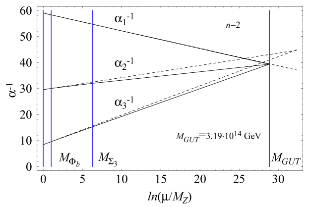
Figure 6: Unification of the gauge couplings at the two-loop level for central values of low-energy observables PDG2004 . The SM case with $n=2$ is presented by dashed lines. Solid lines correspond to the $n=2$ scenario with $\Phi_{b}$ and $\Sigma_{3}$ below the GUT scale. Vertical lines mark the relevant scales: $M_{Z}$, $M_{\Phi_{b}}=250$ GeV, $M_{\Sigma_{3}}=4.95\times 10^{4}$ GeV and $M_{GUT}=3.19\times 10^{14}$ GeV.

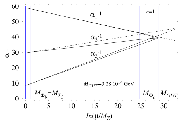
Figure 7: Unification of the gauge couplings at the two-loop level for central values of low-energy observables PDG2004 . The SM case with $n=1$ is presented by dashed lines. Solid lines correspond to the $n=1$ scenario with $\Phi_{b}$, $\Sigma_{3}$ and $\Phi_{a}$ below the GUT scale. Vertical lines mark the relevant scales: $M_{Z}$, $M_{\Phi_{b}}=M_{\Sigma_{3}}=250$ GeV and $M_{GUT}=3.28\times 10^{14}$ GeV.

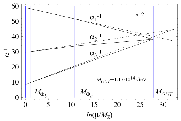
Figure 8: Unification of the gauge couplings at the two-loop level for central values of low-energy observables PDG2004 . The SM case with $n=2$ is presented by dashed lines. Solid lines correspond to the $n=2$ scenario with $\Phi_{b}$ and $\Phi_{a}$ below the GUT scale. Vertical lines mark the relevant scales: $M_{Z}$, $M_{\Phi_{b}}=250$ GeV, $M_{\Phi_{a}}=4.41\times 10^{6}$ GeV and $M_{GUT}=1.17\times 10^{14}$ GeV.

The GUT scale as well as appropriate intermediate scales are indicated on the plots. For example, in the $n=2$ scenario with light $\Sigma_{3}$ in Fig. 6 the GUT scale is close to the one-loop results (see Fig. 1 in particular) and comes out to be $3.19\times 10^{14}$ GeV for central values of coupling constants PDG2004 . The $1\,\sigma$ departure allows for the maximum value of $3.35\times 10^{14}$ GeV in that case. Note that the $n=1$ case with light $\Sigma_{3}$ presented in Fig. 7 yields somewhat higher GUT scale. The reason behind this trend is simple: the $\Phi_{b}$ contribution to $B_{12}$ is seven times that of the Higgs doublet but, at the same time, they contribute the same to $B_{23}$. Thus, $\Phi_{b}$ is more efficient in simultaneously improving the running and raising the GUT scale than any extra Higgs doublets.

One might object that lightness of $\Sigma_{3}$, which requires miraculous fine-tuning, makes the scenario with an extra $\bm{15}$ rather unattractive. Again, we do not insist on $\Sigma_{3}$ being at intermediate scale. Note that the unification with almost the same GUT scale as in the intermediate $\Sigma_{3}$ case is achieved at the two-loop level in the scenario where $\Phi_{a}$ is at intermediate and $\Sigma_{3}$ is at the GUT scale. See Figs. 4 and 8 for the $n=1$ and $n=2$ cases, respectively. As discussed in the text, intermediate scale for $\Phi_{a}$ would require either small Yukawas for Majorana neutrinos or small $c_{3}$. In the latter case, the novel contributions towards proton decay would be automatically suppressed. The former case could be probed if and when the leptoquarks are detected since some of the rare processes involving neutrinos would be significantly suppressed compared with the charged lepton ones. We note that in the scenario with intermediate $\Phi_{a}$ the GUT scale grows with the number of light Higgs doublets in contrast to the case when $\Sigma_{3}$ is at the intermediate scale. Again, the reason is that the $B_{12}$ coefficient of $\Phi_{a}$ is the same as the appropriate coefficient of the Higgs doublet but its contribution to $B_{23}$ is four times bigger. Thus, the very efficiency of $\Phi_{a}$ in improving unification makes its impact on $M_{GUT}$ rather small.

References

- (1) H. Georgi and S. L. Glashow, Phys. Rev. Lett. 32 (1974) 438.
- (2) W. J. Marciano, BNL-34599 Presented at Miniconf. on Low-Energy Tests of Conservation Laws in Particle Physics, Blacksburg, VA, Sep 11-14, 1983
- (3) P. Minkowski, Phys. Lett. B 67 (1977) 421; T. Yanagida, proceedings of the Workshop on Unified Theories and Baryon Number in the Universe, Tsukuba, 1979, eds. A. Sawada, A. Sugamoto, KEK Report No. 79-18, Tsukuba. S. Glashow, in Quarks and Leptons, Cargèse 1979, eds. M. Lévy. et al., (Plenum, 1980, N ew York). M. Gell-Mann, P. Ramond, R. Slansky, proceedings of the Supergravity Stony Brook Workshop, New York, 1979, eds. P. Van Niewenhuizen, D. Freeman (North-Holland, Amsterdam). R. Mohapatra, G. Senjanović, Phys.Rev.Lett. 44 (1980) 912
- (4) G. Lazarides, Q. Shafi and C. Wetterich, Nucl. Phys. B 181 (1981) 287.
- (5) R. N. Mohapatra and G. Senjanovic, Phys. Rev. D 23 (1981) 165.
- (6) S. Weinberg, Phys. Rev. Lett. 43 (1979) 1566.
- (7) R. Barbieri, J. R. Ellis and M. K. Gaillard, Phys. Lett. B 90 (1980) 249.
- (8) E. K. Akhmedov, Z. G. Berezhiani and G. Senjanovic, Phys. Rev. Lett. 69 (1992) 3013 [arXiv:hep-ph/9205230].
- (9) J. R. Ellis and M. K. Gaillard, Phys. Lett. B 88 (1979) 315.
- (10) H. Georgi and C. Jarlskog, Phys. Lett. B 86 (1979) 297.
- (11) P. Nath, Phys. Rev. Lett. 76 (1996) 2218; Phys. Lett. B 381 (1996) 147; B. Bajc, P. Fileviez Pérez and G. Senjanović, arXiv:hep-ph/0210374.
- (12) K. S. Babu and E. Ma, Phys. Lett. B 144 (1984) 381.
- (13) A. Giveon, L. J. Hall and U. Sarid, Phys. Lett. B 271 (1991) 138.
- (14) T. P. Cheng, E. Eichten and L. F. Li, Phys. Rev. D 9 (1974) 2259.
- (15) S. Eidelman et al. [Particle Data Group], Phys. Lett. B 592 (2004) 1.
- (16) H. Murayama and T. Yanagida, Mod. Phys. Lett. A 7 (1992) 147.
- (17) A. J. Buras, J. R. Ellis, M. K. Gaillard and D. V. Nanopoulos, Nucl. Phys. B 135 (1978) 66.
- (18) S. Nandi, A. Stern and E. C. G. Sudarshan, Phys. Lett. B 113 (1982) 165.
- (19) I. Dorsner and P. Fileviez Pérez, arXiv:hep-ph/0410198.
- (20) S. M. Barr, G. Segre and H. A. Weldon, Phys. Rev. D 20 (1979) 2494.
- (21) D. V. Nanopoulos and S. Weinberg, Phys. Rev. D 20 (1979) 2484.
- (22) A. Yildiz and P. Cox, Phys. Rev. D 21 (1980) 906.
- (23) M. Fukugita and T. Yanagida, Phys. Rev. Lett. 89 (2002) 131602 [arXiv:hep-ph/0203194].
- (24) L. F. Li, Phys. Rev. D 9 (1974) 1723.
- (25) A. H. Guth and S. H. H. Tye, Phys. Rev. Lett. 44 (1980) 631 [Erratum-ibid. 44 (1980) 963].
- (26) A. H. Guth and E. J. Weinberg, Phys. Rev. D 23 (1981) 876.
- (27) W. Buchmuller, R. Ruckl and D. Wyler, Phys. Lett. B 191 (1987) 442 [Erratum-ibid. B 448 (1999) 320].
- (28) S. Davidson, D. C. Bailey and B. A. Campbell, Z. Phys. C 61 (1994) 613 [arXiv:hep-ph/9309310].
- (29) M. Herz, arXiv:hep-ph/0301079.
- (30) C. Dohmen et al. [SINDRUM II Collaboration.], Phys. Lett. B 317 (1993) 631.
- (31) S. M. Wang [CDF Collaboration], arXiv:hep-ex/0405075; R. Barate et al. [ALEPH Collaboration], Eur. Phys. J. C 12 (2000) 183 [arXiv:hep-ex/9904011]; P. Abreu et al. [DELPHI Collaboration], Phys. Lett. B 446 (1999) 62 [arXiv:hep-ex/9903072]; M. Acciarri et al. [L3 Collaboration], Phys. Lett. B 489 (2000) 81 [arXiv:hep-ex/0005028]; G. Abbiendi et al. [OPAL Collaboration], Phys. Lett. B 526 (2002) 233 [arXiv:hep-ex/0112024]; G. Abbiendi et al. [OPAL Collaboration], Eur. Phys. J. C 31 (2003) 281 [arXiv:hep-ex/0305053]; S. Chekanov et al. [ZEUS Collaboration], Phys. Rev. D 68 (2003) 052004 [arXiv:hep-ex/0304008].
- (32) V. A. Mitsou, N. C. Benekos, I. Panagoulias and T. D. Papadopoulou, arXiv:hep-ph/0411189.
- (33) S. Abdullin and F. Charles, Phys. Lett. B 464 (1999) 223 [arXiv:hep-ph/9905396].
- (34) M. Kramer, T. Plehn, M. Spira and P. M. Zerwas, arXiv:hep-ph/0411038; A. Belyaev, C. Leroy, R. Mehdiyev and A. Pukhov, arXiv:hep-ph/0502067.
- (35) K. Kobayashi et al. [Super-Kamiokande Collaboration], arXiv:hep-ex/0502026.
- (36) R. N. Mohapatra, Unification and Supersymmetry: The Frontiers of Quark-Lepton Physics, Springer-Verlag, 1986.
- (37) G. C. Branco, Phys. Rev. D 23 (1981) 2702.
- (38) G.C. Branco, L. Lavoura and J.P. Silva, CP violation: Oxford, Clarendon Press, 1999.
- (39) C. Panagiotakopoulos and Q. Shafi, Phys. Rev. Lett. 52 (1984) 2336.
- (40) H. Ruegg, Phys. Rev. D 22 (1980) 2040.
- (41) F. Buccella, G. B. Gelmini, A. Masiero and M. Roncadelli, Nucl. Phys. B 231 (1984) 493.
- (42) P. Fileviez Pérez, Phys. Lett. B 595 (2004) 476 [arXiv:hep-ph/0403286].
- (43) L. J. Hall, Nucl. Phys. B 178 (1981) 75.
- (44) D. R. T. Jones, Phys. Rev. D 25 (1982) 581.