Possible energy dependence of $\Theta_{13}$ in neutrino oscillations

Abstract

A simple three-flavor neutrino-oscillation model is discussed which has both nonzero mass differences and timelike Fermi-point splittings, together with a combined bi-maximal and trimaximal mixing pattern. One possible consequence would be new effects in $\nu_{\mu}\to\nu_{e}$ oscillations, characterized by an energy-dependent effective mixing angle $\Theta_{13}$. Future experiments such as T2K and NO$\nu$A, and perhaps even the current MINOS experiment, could look for these effects.

I Introduction

The standard explanation of neutrino oscillations relies on mass differences GribovPontecorvo ; BilenkyPontecorvo1976 ; BilenkyPontecorvo1978 and two recent reviews can be found in Refs. Barger-etal ; McKeownVogel . There have, of course, been many suggestions for alternative mechanisms; see, e.g., Refs. Gasperini ; Halprin ; ColemanGlashow ; Huber-etal ; KosteleckyMewes ; BarenboimMavromatos and references therein. One possibility motivated by condensed-matter physics would be Fermi-point splitting of the Standard Model fermions due to a new type of quantum phase transition KlinkhamerVolovikJETPL ; KlinkhamerVolovikIJMPA .

The phenomenology of a “radical” neutrino-oscillation model with strictly zero mass differences and nonzero Fermi-point splittings has been discussed in Refs. KlinkhamerJETPL ; Klinkhamer0407200 . A less extreme possibility would be a type of “stealth scenario” with Fermi-point-splitting effects hiding behind mass-difference effects Klinkhamer0407200 . The present article aims to give an exploratory discussion of this last possibility.

Specifically, we consider the case with both mass-square differences $\Delta m^{2}$ and timelike Fermi-point splittings $\Delta b_{0}$. (Timelike Fermi-point splittings preserve spatial isotropy, whereas spacelike splittings give anisotropic neutrino oscillations KlinkhamerJETPL .) There are then two methods to determine the presence of these $\Delta b_{0}$ terms. The first method is to use sufficiently high neutrino energies $E_{\nu}$ so that the mass-difference effects drop out, $|\Delta m^{2}/(2E_{\nu})|\ll|\Delta b_{0}|$ for generic mixing angles. The second method is to look at a particular process which is expected to be small for standard mass-difference neutrino oscillations.

An example of the second method is provided by the standard appearance probability $P(\nu_{\mu}\rightarrow\nu_{e})\propto\sin^{2}(2\theta_{13})$, for small values of the mixing angle $\theta_{13}$ and not too large travel distance $L$. If there are relatively weak Fermi-point splittings in addition to the mass differences, one has a similar expression for $P(\nu_{\mu}\rightarrow\nu_{e})$ but with the “bare” mixing angle $\theta_{13}$ replaced by an effective mixing angle $\Theta_{13}$, which is now a function of the basic parameters. Phenomenologically, the most interesting consequence would be that $\Theta_{13}$ becomes energy dependent. The resulting $\nu_{e}$ energy spectrum near the first oscillation maximum will be discussed in detail for a simple three-flavor model. Let us remark that, quite generally, the goal of the present article is to point out a possible energy dependence of all neutrino-oscillation parameters and the simple three-flavor model is used as an explicit example.

The outline of this article is as follows. Section II gives the basic mechanism for the case of two neutrino flavors. Section III incorporates these results in a simple three-flavor model with a single dimensionless parameter to describe the relative strength of Fermi-point-splitting and mass-difference effects. Section IV addresses certain phenomenological issues and gives possible signatures for planned or proposed superbeam experiments (e.g., T2K or NO$\nu$A). In addition, further model results are given which may be relevant to the current MINOS experiment. Section V contains concluding remarks.

II Two-flavor model

The starting point of our discussion is the following generalized neutrino dispersion relation KlinkhamerVolovikIJMPA :

$$E_{\nu}(\vec{p}\,)=\sqrt{(c_{\nu}\,p+b_{0\nu})^{2}+m_{\nu}^{2}\,c_{\nu}^{4}}\sim c_{\nu}\,p+b_{0\nu}+m_{\nu}^{2}\,c_{\nu}^{3}/(2\,p)\,,$$ (1)

for large enough neutrino momentum $p\equiv|\vec{p}\,|$ and with a maximum neutrino velocity $c_{\nu}$, a timelike Fermi-point-splitting parameter $b_{0\nu}$, and a mass parameter $m_{\nu}$. Now, consider two-flavor vacuum neutrino oscillations from both mass differences and timelike Fermi-point splittings KlinkhamerJETPL ; Klinkhamer0407200 . The relevant energy differences are then obtained from the eigenvalues of the $2\times 2$ Hermitian matrix ColemanGlashow

$$c_{\nu}\,p\,A+B_{0}+M^{2}\,c_{\nu}^{3}/(2\,p)\,,$$ (2)

with $p\equiv|\vec{p}\,|$ and $2\times 2$ Hermitian matrices $A$, $B_{0}$, and $M^{2}$. In our case, we have $A$ equal to the identity matrix, $A=\openone$, and the maximum neutrino velocity $c_{\nu}$ equal to the velocity of light in vacuo, $c_{\nu}=c$. Natural units with $\hbar$ $=$ $c$ $=$ $1$ will be used in the following.

For two neutrino flavors (denoted $f$ and $g$) and large enough beam energy $E_{\nu}$, the survival and appearance probabilities over a travel distance $L$ are given by

$$P(\nu_{f}\rightarrow\nu_{f}) = 1-P(\nu_{f}\rightarrow\nu_{g})\,,$$ (3a)

$$P(\nu_{f}\rightarrow\nu_{g}) \sim \sin^{2}\left(2\,\Theta\right)\;\sin^{2}\left(\Delta E\,L/2\right)\,,$$ (3b)

with $\Delta E\geq 0$ and $\Theta\in[\,0,\pi/2\,]$ defined by ColemanGlashow

$$\Delta E\,\sin 2\,\Theta = |\,\Delta m^{2}/(2E_{\nu})\sin 2\theta+\exp({\rm i}\,2\,\gamma)\;\Delta b\,\sin 2\chi\,|\,,$$ (4a)

$$\Delta E\,\cos 2\,\Theta = \Delta m^{2}/(2E_{\nu})\cos 2\theta+\Delta b\,\cos 2\chi\,.$$ (4b)

Here, $\Delta m^{2}\equiv m_{2}^{2}-m_{1}^{2}$ is the difference of the eigenvalues of the matrix $M^{2}$ and $\theta$ is the related mixing angle. In the same way, $\Delta b\equiv b_{0}^{(2)}-b_{0}^{(1)}$ and $\chi$ come from the matrix $B_{0}$. In addition, there is one relative phase, $\gamma$.

Equations (4ab) make clear that, provided $\Delta m^{2}$ and $\Delta b$ are nonzero, the effective mixing angle $\Theta$ interpolates between a value close to $\chi$ for relatively high beam energy $E_{\nu}$ and a value close to $\theta$ for relatively low beam energy $E_{\nu}$ [but still large enough for Eq. (2) to apply, see also Sec. IV.1]. In order to be more explicit, we restrict ourselves to the two “extreme” values for the mixing angles $\theta$ and $\chi$, namely, the values $0$ and $\pi/4$. We, again, assume that both $\Delta m^{2}$ and $\Delta b$ are nonzero. Three of the four possible cases then lead to neutrino oscillations:

$$\begin{array}[]{lcl}\mathrm{case}\hskip 4.30554pt1:\quad\theta=0&\quad\mathrm{and}&\chi=\pi/4\,,\\ \mathrm{case}\hskip 4.30554pt2:\quad\theta=\pi/4&\quad\mathrm{and}&\chi=\pi/4\,,\\ \mathrm{case}\hskip 4.30554pt3:\quad\theta=\pi/4&\quad\mathrm{and}&\chi=0\,.\end{array}$$ (5)

Since the results for case 3 follow simply from those for case 1, we only need to give the results for cases 1 and 2 (denoted by a single and a double prime, respectively).

Case 1 has appearance probability

$$P^{\prime}(\nu_{f}\rightarrow\nu_{g}) \sim \sin^{2}\left(2\,\Theta^{\prime}\right)\;\sin^{2}\left(\,\Delta E^{\prime}\,L/2\,\right)\,,$$ (6a)

$$\Delta E^{\prime} = \sqrt{(\Delta b)^{2}+(\Delta m^{2}/(2E_{\nu}))^{2}}\,,$$ (6b)

$$2\,\Theta^{\prime} = \arctan\left(\,\frac{|\Delta b|}{\Delta m^{2}/(2E_{\nu})}\,\right)\,,$$ (6c)

with the dependence on phase $\gamma$ dropping out altogether. Observe that the effective mixing angle $\Theta^{\prime}$ is energy dependent, rising from a value $0$ at $E_{\nu}\sim 0$ to a value $\pi/4$ for $E_{\nu}\to\infty$.

Case 2 has survival probability

$$P^{\prime\prime}(\nu_{f}\rightarrow\nu_{f}) \sim 1-\sin^{2}\left(\,\left|\,\exp({\rm i}\,2\,\gamma)\;\Delta b+\Delta m^{2}/(2E_{\nu})\,\right|\,L/2\,\right)\,,$$ (7)

with a constant mixing angle $\Theta^{\prime\prime}=\pi/4$. Observe that the probabilities are $\gamma$ dependent. In fact, neutrino oscillations at energies $E_{\nu}=|\Delta m^{2}/(2\Delta b)|$ are entirely suppressed for $\gamma=\pi/2$ or $0$, depending on the relative sign of $\Delta b$ and $\Delta m^{2}$.

Case 3 has a survival probability $P^{\prime\prime\prime}$ and effective mixing angle $\Theta^{\prime\prime\prime}$ given by (6abc) with $\Delta b$ and $\Delta m^{2}/(2E_{\nu})$ interchanged. This implies that $\Theta^{\prime\prime\prime}$ has a value $\pi/4$ at $E_{\nu}\sim 0$ and vanishes for $E_{\nu}\to\infty$.

With the heuristics of the two-flavor case established, we turn to the more complicated three-flavor case in the next section.

III Three-flavor model

For three neutrino flavors, the diagonalization of the energy matrix (2), now in terms of $3\times 3$ Hermitian matrices $A=\openone$, $B_{0}$, and $M^{2}$, gives many more mixing angles and phases than for the two-flavor case. Using Iwasawa decompositions of the relevant $SU(3)$ matrices, one has the following parameters: $\{\theta_{21},\theta_{32},\theta_{13},\delta\}$ for an $SU(3)$ matrix $X$ from $M^{2}$, $\{\chi_{21},\chi_{32},\chi_{13},\epsilon\}$ for an $SU(3)$ matrix $Y$ from $B_{0}$, and $\{\alpha,\beta\}$ for a diagonal phase-factor matrix $P$ generated by the Cartan subalgebra.

Specifically, the matrices $P$ and $N=X,Y$ are defined as follows:

$$P \equiv \mathrm{diag}\left(\,{\rm e}^{{\rm i}\beta}\,,\,{\rm e}^{-{\rm i}(\alpha+\beta)}\,,\,{\rm e}^{{\rm i}\alpha}\,\right)\equiv\left(\begin{array}[]{ccc}{\rm e}^{{\rm i}\beta}&0&0\\ 0&{\rm e}^{-{\rm i}(\alpha+\beta)}&0\\ 0&0&{\rm e}^{{\rm i}\alpha}\end{array}\right)\,,$$ (8d)

$$N \equiv \left(\begin{array}[]{ccc}1&0&0\\ 0&c_{32}&s_{32}\\ 0&-s_{32}&c_{32}\end{array}\right)\cdot\left(\begin{array}[]{ccc}c_{13}&0&\;+s_{13}\,{\rm e}^{+i\omega}\\ 0&1&0\\ -s_{13}\,{\rm e}^{-i\omega}&0&c_{13}\end{array}\right)\cdot\left(\begin{array}[]{ccc}c_{21}&s_{21}&0\\ -s_{21}&c_{21}&0\\ 0&0&1\end{array}\right)\,,$$ (8n)

with $\{s_{ij},c_{ij},\omega\}$ equal to $\{\sin\theta_{ij},\cos\theta_{ij},\delta\}$ for the matrix $N=X$ and to $\{\sin\chi_{ij},\cos\chi_{ij},\epsilon\}$ for the matrix $N=Y$. The relevant terms of the Hamiltonian in the flavor basis are then

$$D_{p}+X\,D_{m}\,X^{-1}+P\,Y\,D_{b_{0}}\,Y^{-1}\,P^{-1}\,,$$ (9)

with diagonal matrices

$$D_{p}\equiv\mathrm{diag}\left(\,p\,,\,p\,,\,p\,\right)\,,\quad D_{m}\equiv\mathrm{diag}\left(\,\frac{m^{2}_{1}}{2p}\,,\,\frac{m^{2}_{2}}{2p}\,,\,\frac{m^{2}_{3}}{2p}\,\right)\,,\quad D_{b_{0}}\equiv\mathrm{diag}\left(\,b_{0}^{(1)}\,,\,b_{0}^{(2)}\,,\,b_{0}^{(3)}\,\right)\,,$$ (10)

for $p\equiv|\vec{p}\,|$ and $c_{\nu}=c=1$. For later use, we already define the differences $\Delta m_{ij}^{2}\equiv m_{i}^{2}-m_{j}^{2}$ and $\Delta b_{0}^{(ij)}\equiv b_{0}^{(i)}-b_{0}^{(j)}$.

The structure of the vacuum neutrino-oscillation probabilities is the same as for the standard case ($D_{b_{0}}=0$); see, e.g., Eqs. (7)–(10) of Ref. Barger-etal . These probabilities are given in terms of six parameters $\Delta E_{21}$, $\Delta E_{31}$, $\Theta_{21}$, $\Theta_{32}$, $\Theta_{13}$, and $\Delta$, which are now complicated functions of the fourteen original parameters $\Delta m^{2}_{21}/(2p)$, $\Delta m^{2}_{31}/(2p)$, $\Delta b_{0}^{(21)}$, $\Delta b_{0}^{(31)}$, $\theta_{21}$, $\theta_{32}$, $\theta_{13}$, $\delta,\chi_{21}$, $\chi_{32}$, $\chi_{13}$, $\epsilon$, $\alpha$, and $\beta$.

In order to illustrate the basic idea and to use the two-flavor results of the previous section, we consider a specific model with the following mass-term differences and bi-maximal mixing angles:

$$\Delta m^{2}_{21}/(2p) = 0\,,\quad\Delta m^{2}_{31}/(2p)\equiv\Delta\mu>0\,,$$ (11a)

$$\theta_{13} = 0\,,\quad\theta_{21}=\theta_{32}=\pi/4\,,$$ (11b)

a similar pattern of timelike Fermi-point splittings and trimaximal mixing angles:

$$\Delta b_{0}^{(21)} = 0\,,\quad\Delta b_{0}^{(31)}\equiv\Delta b_{0}>0\,,$$ (12a)

$$\chi_{13} = \chi_{21}=\chi_{32}=\pi/4\,,$$ (12b)

and vanishing phases:

$$\delta=\epsilon=\alpha=\beta=0\,.$$ (13)

The values (11ab) are more or less standard with $|\Delta m^{2}_{31}|\approx 2.5\times 10^{-3}\;{\rm eV}^{2}$; cf. Refs. Barger-etal ; McKeownVogel . The actual values of $\theta_{21}$ and $\chi_{21}$ are, in fact, irrelevant for the case $\Delta m^{2}_{21}=\Delta b_{0}^{(21)}=0$. As it stands, the simple model depends on only one positive dimensionless parameter, $\Delta b_{0}/\Delta\mu$.

Explicit expressions for the energy eigenvalues $E_{n}$ of the corresponding matrix (9) are readily obtained and give the following differences:

$$\Delta E_{21} \equiv E_{2}-E_{1}={\textstyle\frac{1}{2}}\left(\Delta\mu+\Delta b_{0}-\sqrt{\Delta\mu^{2}+\Delta b_{0}^{2}}\right)\,,$$ (14a)

$$\Delta E_{31} \equiv E_{3}-E_{1}={\textstyle\frac{1}{2}}\left(\Delta\mu+\Delta b_{0}+\sqrt{\Delta\mu^{2}+\Delta b_{0}^{2}}\right)\,.$$ (14b)

The most important result for us is that $|\Delta E_{21}/\Delta E_{31}|\lesssim 10\%\,$ for $\Delta b_{0}\lesssim 0.2\,\Delta\mu$. In the following discussion, we assume $0<\Delta b_{0}\ll\Delta\mu$, which allows us to use simplified expressions for the oscillation probabilities; cf. Refs. Barger-etal ; McKeownVogel . (Note that the approximation $\Delta b_{0}\gg\Delta\mu>0$ would be equally simple.)

In the context of three-flavor neutrino oscillations, case 1 of Eq. (5) with $\theta=0$ may be relevant to the $\theta_{13}$ mixing angle, which is known to be rather small from the CHOOZ CHOOZ and Palo Verde PaloVerde2001 experiments. For three-flavor parameters (11)–(13), large enough beam energy $E_{\nu}$, and not too large travel distance ($L\Delta b_{0}\ll L\Delta\mu\lesssim 1$), the $\nu_{\mu}\rightarrow\nu_{e}$ appearance probability is essentially given by Eq. (6) and reads

$$P_{\mu e} \equiv P(\nu_{\mu}\rightarrow\nu_{e})\sim{\textstyle\frac{1}{2}}\,\sin^{2}\left(2\,\Theta_{13}\right)\;\sin^{2}\left(\,\Delta E_{31}\,L/2\,\right)+\mathrm{O}\left(\left(\Delta b_{0}\,L\right)^{2}\right)\,,$$ (15a)

$$2\,\Theta_{13} \sim \arctan\left(\frac{\Delta b_{0}}{\Delta\mu}\right)+\mathrm{O}\left(\left(\Delta b_{0}/\Delta\mu\right)^{2}\right)\,,$$ (15b)

with $\Delta E_{31}$ given by expression (14b). Analytically, the omitted terms in Eq. (15a) would be negligible if the “bare” mixing angle $\theta_{13}$ were small but finite. But, for the simple model considered with $\theta_{13}=0$ exactly, the omitted terms could, in principle, be important and only a comparison with the full numerical result can be conclusive (see Sec. IV.2).

Case 2 of Eq. (5) with $\theta=\pi/4$, on the other hand, may be relevant to the $\theta_{32}$ mixing angle, which is known to be nearly maximal from the SK results SuperK1998 ; SuperK2005 . For three-flavor parameters (11)–(13), large enough beam energy $E_{\nu}$, and not too large travel distance $L$, the $\mu$–type survival probability is essentially given by Eq. (7) and reads

$$P_{\mu\mu} \equiv P(\nu_{\mu}\rightarrow\nu_{\mu})\sim 1-\sin^{2}\left(\,\Delta E_{31}\,L/2\,\right)+\mathrm{O}\left(\Delta b_{0}\,\Delta\mu\,L^{2}\right)\,,$$ (16)

again with $\Delta E_{31}$ given by expression (14b). Typically, one expects $\mathrm{O}\left(\Delta b_{0}/\Delta\mu\right)$ corrections to the probabilities. There could also be interesting effects for an extended version of the model with nonzero phases $\alpha$ and $\beta$, as mentioned a few lines below Eq. (7). But, these issues will not be pursued further here.

IV Phenomenology

IV.1 Preliminaries

In order to connect with future experiments which aim to determine or constrain the standard energy-independent mixing angle $\theta_{13}$, consider the appearance probability (15) from the simple model (8)–(13). For relatively weak Fermi-point splitting, $0<\Delta b_{0}\equiv\Delta b_{0}^{(31)}\ll\Delta\mu\equiv\Delta m^{2}_{31}/(2p)$, the effective mixing angle $\Theta_{13}$ then has a linear dependence on the neutrino beam energy $E_{\nu}\sim p\equiv|\vec{p}\,|$ and is given by

$$\Theta_{13}\sim\frac{E_{\nu}}{\Delta m^{2}_{31}}\;\Delta b_{0}^{(31)}+\mathrm{O}\left(\left(\Delta b_{0}/\Delta\mu\right)^{2}\right)\,,$$ (17)

since the argument of the arctangent function in Eq. (15b) is positive. If experiment can now establish an upper bound $\Delta\Theta_{13}$ on the variation of $\Theta_{13}(E)$ over an energy range $\Delta E_{\nu\,\mathrm{range}}$, one obtains an upper bound on $\Delta b_{0}$. From Eq. (17), one has

$$|\Delta b_{0}^{(31)}| \lesssim |\Delta m^{2}_{31}\;\Delta\Theta_{13}/\Delta E_{\nu\,\mathrm{range}}|$$ (18)

$$\approx 6\times 10^{-13}\;{\rm eV}\,\left(\frac{|\Delta m^{2}_{31}|}{2.5\times 10^{-3}\;{\rm eV}^{2}}\right)\,\left(\frac{\sin^{2}(2\Delta\Theta_{13})}{0.05}\right)^{\!1/2}\,\left(\frac{0.5\;{\rm GeV}}{|\Delta E_{\nu\,\mathrm{range}}|}\right)\,,$$

with more or less realistic values inserted for the planned T2K experiment T2K (for the proposed NO$\nu$A experiment NOvA , the energy range could be four times larger, giving a four times smaller upper bound for the Fermi-point splitting).

A next-generation superbeam BNL2002 ; Kobayashi or neutrino factory Geer1997 ; Blondel2004 could perhaps reach a $10^{2}$ times better sensitivity than shown in Eq. (18), assuming $\sin^{2}(2\Delta\Theta_{13})\approx 0.002$ and $\Delta E_{\nu\,\mathrm{range}}\approx 10\;{\rm GeV}$. New reactor experiments Whitepaper , however, would operate at lower energies and would have less sensitivity by a factor of $10^{2}$, assuming $\sin^{2}(2\Delta\Theta_{13})\approx 0.05$ and $\Delta E_{\nu\,\mathrm{range}}\approx 5\;{\rm MeV}$. As mentioned before, the neutrino energy $E_{\nu}$ must still be large enough for Eqs. (1),(2), and (9) to apply, which we take to mean $E_{\nu}\gg 1\;\mathrm{keV}$, based on the absolute bound $|b_{0}^{(e)}|\leq 1\;\mathrm{keV}$ reported in Ref. DiGrezia-etal , the conservative differential bounds $|\Delta b_{0}^{(ij)}|\leq 10^{-11}\;\mathrm{eV}$ from Refs. KlinkhamerJETPL ; Klinkhamer0407200 , and the absolute bound $\sum_{i}m_{i}\leq 10^{2}\;\mathrm{eV}$ from cosmology Barger-etal ; McKeownVogel .

Since there could be Fermi-point-splitting effects hiding in the existing neutrino oscillation data with $|\Delta b_{0}|$ of the order of $10^{-12}\;{\rm eV}$ KlinkhamerJETPL ; Klinkhamer0407200 , superbeam experiments T2K ; NOvA ; BNL2002 ; Kobayashi look the most promising in the near future, as neutrino factories may very well remain in the R&D phase for at least 10 years. In Sec. IV.2, we, therefore, expand on the appearance probability $P(\nu_{\mu}\rightarrow\nu_{e})$ at forthcoming off-axis superbeam experiments which can be expected to have relatively good control of the backgrounds. In Sec. IV.3, we also discuss this appearance probability for the on-axis MINOS experiment which can have relatively high neutrino energies.

IV.2 Model results near the first oscillation maximum

In this subsection, we consider the appearance probability $P_{\mu e}\equiv P(\nu_{\mu}\rightarrow\nu_{e})$ from the simple model (8)–(13) with both mass-square differences and timelike Fermi-point splittings. Experimentally, there are two important parameters to determine from the measured values of the quantity $P_{\mu e}=P_{\mu e}(L,E_{\nu})$, namely $\Delta m^{2}_{31}$ and $\Delta b_{0}^{(31)}$, where $|\Delta b_{0}^{(31)}|$ is assumed to be less than $|\Delta m^{2}_{31}|/(2E_{\nu})$ for typical energies $E_{\nu}$. Perhaps the simplest way to determine or constrain $|\Delta b_{0}^{(31)}|$ would be to place the far detector close to the first oscillation maximum corresponding to the average energy $\overline{E}_{\nu}$. The near detector close to the source determines the initial $\nu_{\mu}$ flux. The idea is then to measure the $\nu_{e}$ energy spectrum in the far detector and to compare with the standard predictions.

The shape of $P_{\mu e}$ vs. $E_{\nu}$ for our combined mass-difference and Fermi-point-splitting (MD+FPS) model is, indeed, different from the one of the standard mass-difference (MD) model. Defining

$$\overline{L} \equiv \pi\;\frac{2\,\overline{E}_{\nu}}{|\Delta m^{2}_{31}|}\approx 295\;\mathrm{km}\,\left(\frac{\overline{E}_{\nu}}{0.5948\;\mathrm{GeV}}\right)\,\left(\frac{2.5\times 10^{-3}\;{\rm eV}^{2}}{|\Delta m^{2}_{31}|}\right),$$ (19a)

$$\overline{\Theta}_{13} \equiv \overline{E}_{\nu}\,\frac{|\Delta b_{0}^{(31)}|}{|\Delta m^{2}_{31}|}\approx 0.0952\,\left(\frac{\overline{E}_{\nu}}{0.5948\;\mathrm{GeV}}\right)\left(\frac{|\Delta b_{0}^{(31)}|}{4\times 10^{-13}\;\mathrm{eV}}\right)\left(\frac{2.5\times 10^{-3}\;{\rm eV}^{2}}{|\Delta m^{2}_{31}|}\right),$$ (19b)

$$l \equiv L/\overline{L}\,,$$ (19c)

$$x \equiv E_{\nu}/\overline{E}_{\nu}\,,$$ (19d)

the approximate model probability (15) becomes

$$P_{\mu e}^{\mathrm{\,MD+FPS}}(l,x) \sim {\textstyle\frac{1}{2}}\,\sin^{2}(2\,\Theta_{13})\;\sin^{2}\left(\frac{\pi}{4}\left[\>x^{-1}+2\,\overline{\Theta}_{13}+\sqrt{x^{-2}+\left(2\,\overline{\Theta}_{13}\right)^{2}}\;\right]\,l\,\right),$$ (20a)

$$2\,\Theta_{13} \sim \arctan(2\,\overline{\Theta}_{13}\,x)\,.$$ (20b)

For comparison, the standard mass-difference result for $m_{1}^{2}=m_{2}^{2}\neq m_{3}^{2}$ and $\theta_{32}=\pi/4$ is given by GribovPontecorvo ; BilenkyPontecorvo1976 ; BilenkyPontecorvo1978 ; Barger-etal ; McKeownVogel

$$P_{\mu e}^{\mathrm{\,MD}}(l,x) = {\textstyle\frac{1}{2}}\,\sin^{2}(2\theta_{13})\;\sin^{2}\left(\,\frac{\pi}{2\,x}\;l\,\right)\,,$$ (21)

with constant mixing angle $\theta_{13}$.

Figure 1 compares the shape of the model probability (20) to the standard result (21), both evaluated at $l\equiv L/\overline{L}=1$. The approximate model probabilities from Eq. (20) [thin broken curves in Fig. 1] are quite reliable for $x\approx 1$ but overshoot by some $40\,\%$ for larger values of $x$, as follows by comparison to the full numerical results [thin solid curves in Fig. 1] which monotonically approach a constant value as $x\to\infty$. Note, however, that this asymptotic value $P={\textstyle\frac{1}{2}}\,\sin^{2}(\pi\,\overline{\Theta}_{13})={\textstyle\frac{1}{2}}\,\sin^{2}(\Delta b_{0}\,\overline{L}/2)$ is correctly reproduced by the approximation (20a) for $l=1$ and $1/x=0$. The analytic expression (20a) can, therefore, be used to get rough estimates. (For corresponding probabilities in another model, see Fig. 8 in Ref. Klinkhamer0407200 .)

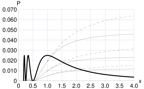
Figure 1: Fixed-distance probabilities $P(\nu_{\mu}\rightarrow\nu_{e})$ at $l\equiv L/\overline{L}=1$ vs. dimensionless energy $x\equiv E_{\nu}/\overline{E}_{\nu}$ for the simple model (8)–(13) with both mass differences and Fermi-point splittings [thin broken and solid curves] and for the standard mass-difference model without Fermi-point splittings [heavy solid curve with maxima $P=0.025$ at $x\leq 1$, the plot being suppressed for $x\leq 0.175\,$]. The thin broken curves and the heavy solid curve are given by the analytic expressions (20) and (21), respectively, with parameters $\sin^{2}(2\overline{\Theta}_{13})=0.01,\,0.02,\,0.04$, and $\sin^{2}(2\theta_{13})=0.05$. The thin broken curves are only approximate for $x\overline{\Theta}_{13}=\mathrm{O}(1)$ and the corresponding thin solid curves give the full numerical results.

The $\nu_{e}$ energy spectrum at $L=\overline{L}$ depends on the initial $\nu_{\mu}$ spectrum at $L=0$, assuming negligible contamination by $\nu_{e}$’s. (Note that, for a real experiment, backgrounds are better controlled in the off-axis configuration than in the on-axis configuration T2K ; NOvA .) As an example, we take for this initial $\nu_{\mu}$ spectrum the following function [cf. upper heavy solid curve in Fig. 2 ]:

$$\left.f_{\mu}(x)\right|_{\,L=0}=\left\{\begin{array}[]{ll}\sin^{2}(x\,\pi/2)\,,&\;\;\mbox{for $x\in[0,1)$}\,,\\[11.38109pt] \exp\left[-(x-1)^{2}\,\right]\,,&\;\;\mbox{for $x\in[1,\infty)$}\,,\end{array}\right.$$ (22)

in terms of the dimensionless energy $x$ from Eq. (19d) and with an arbitrary normalization. The $\nu_{e}$ spectrum at $L=\overline{L}$ (or $l=1$) is then given by

$$\left.f_{e}(x)\right|_{\,L=\overline{L}}=\left.f_{\mu}(x)\right|_{\,L=0}\;P_{\mu e}(1,x)\,.$$ (23)

Figure 2 shows the resulting $\nu_{e}$ energy spectra: the lower heavy solid curve corresponds to the probability (21) of the standard mass-difference model and the thin solid (broken) curves correspond to the numerical (approximate) probabilities of the simple model with both mass differences and Fermi-point splittings, the approximate probability being given by Eq. (20a).

The reader is invited to compare the solid curves of Fig. 2 with Figs. 6b and 13a of Ref. T2K for T2K, which give the initial $\nu_{\mu}$ spectrum and the expected $\nu_{e}$ signal for mass-difference oscillations with $\sin^{2}(2\theta_{13})=0.1$ (i.e., twice the value used in our figures). T2K would appear to be able to measure the oscillation probability (20) for $\sin^{2}(2\overline{\Theta}_{13})=0.04$, which corresponds to $|\Delta b_{0}^{(31)}|\approx 4\times 10^{-13}\;\mathrm{eV}$, according to Eq. (19b) for $\overline{E}_{\nu}=0.6\;\mathrm{GeV}$ and $\Delta m^{2}_{31}=2.5\times 10^{-3}\;{\rm eV}^{2}$. The proposed NO$\nu$A experiment NOvA would be sensitive to approximately four times smaller values of the Fermi-point splitting, $|\Delta b_{0}^{(31)}|\approx 10^{-13}\;\mathrm{eV}$, because of the approximately four times higher energy, even though $L\approx 810\;\mathrm{km}$ is a bit short of $\overline{L}\approx 1200\;\mathrm{km}$. (For a generalized model with $\theta_{13}=0$ exactly and $\chi_{13}$ arbitrary, similar sensitivities hold for the quantity $|\Delta b_{0}^{(31)}\,\sin 2\chi_{13}|\,$.)

The sensitivity is one issue but the ability to choose between different models is another. In fact, it would not be easy to distinguish between the standard mass-difference model with $\sin^{2}2\theta_{13}=0.05$ [lower heavy solid curve of Fig. 2 ] and the combined mass-difference and Fermi-point-splitting model with $\theta_{13}=0$ and $\sin^{2}(2\overline{\Theta}_{13})=0.04$ [upper thin solid curve of Fig. 2 ]. Possible signatures of the simple model (8)–(13) for the $\nu_{e}$ energy spectrum at $L=\overline{L}$ would be a shift of the initial $x=1$ peak to $x\approx 1.4$, practically zero activity for $x\lesssim 0.5$, and an enhanced signal for $x\gtrsim 2$.

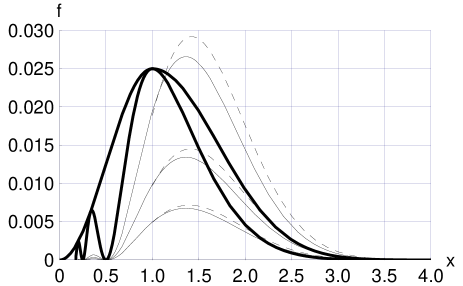
Figure 2: Electron–type neutrino energy spectra $f_{e}(x)$ at $l\equiv L/\overline{L}=1$ from an initial muon–type spectrum (22) at $l=0$ and probabilities $P(\nu_{\mu}\rightarrow\nu_{e})$ of Fig. 1. The initial $\nu_{\mu}$ spectrum multiplied by a constant factor $0.025$ is shown as the upper heavy solid curve. The $\nu_{e}$ spectra at $l=1$ are shown as the lower heavy solid curve for the standard mass-difference model ($\sin^{2}\,2\theta_{13}=0.05$) and as the thin broken and solid curves for the simple model with both mass differences ($\theta_{13}=0$) and Fermi-point splittings (see Fig. 1 for further details).

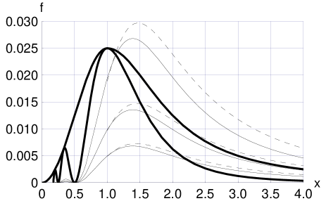
Figure 3: Same as Fig. 2, but now for initial muon-type neutrino energy spectrum (24).

Expanding on this last point, it is clear that an initial energy spectrum with a pronounced high-energy tail would be advantageous. As an example, we take the following function [cf. upper heavy solid curve in Fig. 3 ]:

$$\left.\widetilde{f}_{\mu}(x)\right|_{\,L=0}=\left\{\begin{array}[]{ll}\sin^{2}(x\,\pi/2)\,,&\;\;\mbox{for $x\in[0,1)$}\,,\\[11.38109pt] 1/\left[1+(x-1)^{2}\,\right]\,,&\;\;\mbox{for $x\in[1,\infty)$}\,,\end{array}\right.$$ (24)

which has an area larger than the one from Eq. (22) by a factor $(1+\pi)/(1+\sqrt{\pi})\approx 1.5$. Figure 3 shows the resulting $\nu_{e}$ energy spectra from Eq. (23) with $f_{\mu}(x)$ replaced by $\widetilde{f}_{\mu}(x)$. In this case, the new-physics signal at $x\approx 2$ would be quite strong, being approximately three times larger for the combined mass-difference and Fermi-point-splitting model with $\theta_{13}=0$ and $\sin^{2}(2\overline{\Theta}_{13})=0.04$ [upper thin solid curve of Fig. 3 ] than for the standard mass-difference model with $\sin^{2}(2\theta_{13})=0.05$ [lower heavy solid curve of Fig. 3 ].

In order to distinguish Fermi-point-splitting effects from mass-difference effects, it is clearly preferable to use a (pure) $\mu$–type neutrino beam with a broad energy spectrum and high average energy. For this reason, we take a closer look at the potential of the current MINOS experiment in the next subsection.

IV.3 Model results short of the first oscillation maximum

In this subsection, we give model results which may be relevant to the on-axis MINOS experiment MINOS1998 ; MINOS2005 with baseline $L=735\;\mathrm{km}$. In order to be specific, we focus on the medium energy (ME) mode of MINOS with an average beam energy of approximately $\overline{E}_{\nu}=7.5\;\mathrm{GeV}$, but the results are qualitatively the same for the low-energy (LE) and high-energy (HE) modes with $\overline{E}_{\nu}$ approximately equal to $3.75\;\mathrm{GeV}$ and $15\;\mathrm{GeV}$, respectively. The average energy $\overline{E}_{\nu}=7.5\;\mathrm{GeV}$ corresponds to a length scale $\overline{L}\approx 3720\;\mathrm{km}$, according to Eq. (19a) for $\Delta m^{2}_{31}=2.5\times 10^{-3}\;{\rm eV}^{2}$.

The approximate probability for the simple model (8)–(13) is again given by Eq. (20). Figure 4 shows the approximate probabilities and the full numerical results as thin broken and thin solid curves, respectively, for model parameters $l\equiv L/\overline{L}=735/3720$ and $\overline{\Theta}_{13}=(0.3,\,0.6,\,0.9)$, which correspond to $\Delta b_{0}\approx(1,\,2,\,3)\times 10^{-13}\;\mathrm{eV}$, according to Eq. (19b) for $\overline{E}_{\nu}=7.5\;\mathrm{GeV}$ and $\Delta m^{2}_{31}=2.5\times 10^{-3}\;{\rm eV}^{2}$. The results for the LE and HE modes of MINOS are similar for $x\gtrsim 1$, because the asymptotic value $P={\textstyle\frac{1}{2}}\,\sin^{2}(\Delta b_{0}\,L/2)$ is independent of the beam energy (for corresponding probabilities in another model, see Fig. 7 in Ref. Klinkhamer0407200 ).

Note that the standard mass-difference probability (21) at $x=1$ is less than $1\,\%$ for $l=735/3720$ and $\sin^{2}(2\theta_{13})=0.2$, which is just above the $90\,\%$ CL limit (analysis A at $\Delta m^{2}=2.5\times 10^{-3}\;{\rm eV}^{2}$) from CHOOZ CHOOZ . This standard probability is shown as the heavy solid curve in Fig. 4.

Figure 5 gives the resulting $\nu_{e}$ energy spectra for an initial $\mu$–type spectrum (24). Again, the results are qualitatively the same for the LE and HE energy-modes of MINOS, but the expected event rates for the HE mode would be larger than for the ME mode and the spectrum would also be somewhat broader.

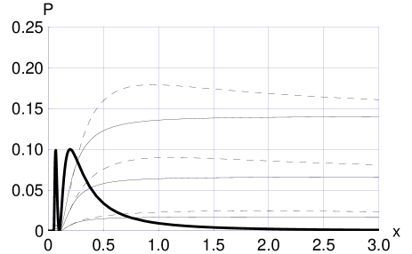
Figure 4: Fixed-distance probabilities $P(\nu_{\mu}\rightarrow\nu_{e})$ at $l\equiv L/\overline{L}=735/3720$ vs. dimensionless energy $x\equiv E_{\nu}/\overline{E}_{\nu}$ for the simple model (8)–(13) with both mass differences and Fermi-point splittings. The thin broken curves are given by the analytic expression (20) with parameters $\overline{\Theta}_{13}=0.3,\,0.6,\,0.9$. The thin broken curves are only approximate for $x\overline{\Theta}_{13}=\mathrm{O}(1)$ and the corresponding thin solid curves give the full numerical results. The heavy solid curve gives, for comparison, the standard mass-difference probability (21) for $\sin^{2}(2\theta_{13})=0.2$ and $l=735/3720$.

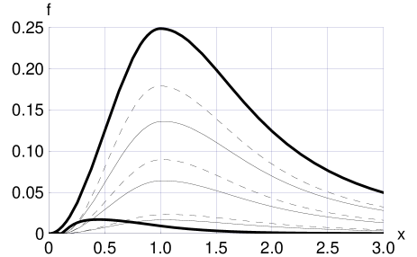
Figure 5: Electron–type neutrino energy spectra $f_{e}(x)$ at $l\equiv L/\overline{L}=735/3720$ from an initial muon–type spectrum (24) at $l=0$ and probabilities $P(\nu_{\mu}\rightarrow\nu_{e})$ of Fig. 4. The initial $\nu_{\mu}$ spectrum multiplied by a constant factor $0.25$ is shown as the upper heavy solid curve. The $\nu_{e}$ spectra are shown as the thin solid curves [approximate values as thin broken curves] for the simple model with both mass differences ($\theta_{13}=0$) and Fermi-point splittings (see Fig. 4 for further details). The lower heavy solid curve gives, for comparison, the $\nu_{e}$ spectrum from the standard mass-difference mechanism with $\sin^{2}(2\theta_{13})=0.2$ and $l=735/3720$.

To summarize, if MINOS in the ME mode is able to place an upper limit on the appearance probability $P(\nu_{\mu}\rightarrow\nu_{e})$ of the order of $5\,\%$, this would correspond to an upper limit on $|\Delta b_{0}^{(31)}\,\sin 2\chi_{13}|$ of the order of $2\times 10^{-13}\;\mathrm{eV}$ (and a factor two better in the HE mode). Moreover, any signal at the $5\,\%$ level or more for $x\gtrsim 1$ would indicate nonstandard (Fermi-point-splitting?) physics, since, as mentioned above, the standard mass-difference probability can be expected to be at most $1\,\%$.

V Conclusion

In this article, we have considered a simple neutrino-oscillation model (8)–(13) with both nonzero mass-square differences ($m^{2}_{1}=m^{2}_{2}\neq m^{2}_{3}$) and timelike Fermi-point splittings ($b_{0}^{(1)}=b_{0}^{(2)}\neq b_{0}^{(3)}$), together with a combined bi-maximal and trimaximal mixing pattern. We expect our basic conclusions to carry over to a more general model with, for example, nonzero phases $\delta,\epsilon,\alpha,\beta,$ and all values of $m^{2}_{n}$ and $b_{0}^{(n)}$ different. As mentioned in the Introduction, the main goal of the present article has been to point out a possible energy dependence of all neutrino-oscillation parameters (for three flavors: three mixing angles $\Theta_{ij}$ and one phase $\Delta$, in addition to the two eigenvalue differences $\Delta E_{ij}$).

Taking the $\theta_{13}$ angle of the mass-square matrix in the simple model to be $0$ (or very small) and the $\chi_{13}$ angle of the Fermi-point-splitting matrix to be $\pi/4$ (or very close to maximal), we have calculated the energy-dependent effective mixing angle $\Theta_{13}$ for the $\nu_{\mu}\to\nu_{e}$ appearance probability. This probability $P(\nu_{\mu}\to\nu_{e})$ is approximately given by Eq. (15) and, near the first oscillation maximum, by Eq. (20) for $l\equiv L/\overline{L}=1$ and Fig. 1. The resulting $\nu_{e}$ energy spectra are shown in Figs. 2 and 3 for different initial $\nu_{\mu}$ energy spectra. Similar results at a smaller value of the dimensionless distance $l$ have been presented in Figs. 4 and 5.

These results show that, even for a (simple) model with Fermi-point splittings hiding behind mass differences, a value $\theta_{13}\approx 0$ would allow for a detection of $|\Delta b_{0}^{(31)}\,\sin 2\chi_{13}|$ at the level of $10^{-13}\;\mathrm{eV}$ in a NO$\nu$A–type experiment. But, it is also possible that MINOS can already place tight upper bounds on (or make the discovery of) Fermi-point splitting, provided the backgrounds are under control.

References

• (1) V.N. Gribov and B. Pontecorvo, “Neutrino astronomy and lepton charge,” Phys. Lett. B 28, 493 (1969).
• (2) S.M. Bilenky and B. Pontecorvo, “Quark–lepton analogy and neutrino oscillations,” Phys. Lett. B 61, 248 (1976).
• (3) S.M. Bilenky and B. Pontecorvo, “Lepton mixing and neutrino oscillations,” Phys. Rept.  41, 225 (1978).
• (4) V. Barger, D. Marfatia, and K. Whisnant, “Progress in the physics of massive neutrinos,” Int. J. Mod. Phys. E 12, 569 (2003) [hep-ph/0308123].
• (5) R.D. McKeown and P. Vogel, “Neutrino masses and oscillations: Triumphs and challenges,” Phys. Rept. 394, 315 (2004) [hep-ph/0402025].
• (6) M. Gasperini, “Testing the principle of equivalence with neutrino oscillations,” Phys. Rev. D 38, 2635 (1988).
• (7) A. Halprin, C. N. Leung, and J. Pantaleone, “A possible violation of the equivalence principle by neutrinos,” Phys. Rev. D 53, 5365 (1996) [hep-ph/9512220].
• (8) S. Coleman and S.L. Glashow, “High-energy tests of Lorentz invariance,” Phys. Rev. D 59, 116008 (1999) [hep-ph/9812418].
• (9) P. Huber, T. Schwetz, and J.W.F. Valle, “Confusing non-standard neutrino interactions with oscillations at a neutrino factory,” Phys. Rev. D 66, 013006 (2002) [hep-ph/0202048].
• (10) V.A. Kostelecký and M. Mewes, “Lorentz and CPT violation in neutrinos,” Phys. Rev. D 69, 016005 (2004) [hep-ph/0309025].
• (11) G. Barenboim and N.E. Mavromatos, “CPT violating decoherence and LSND: A possible window to Planck scale physics,” JHEP 01, 034 (2005) [hep-ph/0404014].
• (12) F.R. Klinkhamer and G.E. Volovik, “Quantum phase transition for the BEC–BCS crossover in condensed matter physics and CPT violation in elementary particle physics,” JETP Lett. 80, 343 (2004) [cond-mat/0407597].
• (13) F.R. Klinkhamer and G.E. Volovik, “Emergent CPT violation from the splitting of Fermi points,” to appear in Int. J. Mod. Phys. A [hep-th/0403037].
• (14) F.R. Klinkhamer, “Neutrino oscillations from the splitting of Fermi points,” JETP Lett. 79, 451 (2004) [hep-ph/0403285].
• (15) F.R. Klinkhamer, “Lorentz-noninvariant neutrino oscillations: Model and predictions,” to appear in Int. J. Mod. Phys. A [hep-ph/0407200].
• (16) M. Apollonio et al. [CHOOZ Collaboration], “Limits on neutrino oscillations from the CHOOZ experiment,” Phys. Lett. B 466, 415 (1999) [hep-ex/9907037]; “Search for neutrino oscillations on a long base-line at the CHOOZ nuclear power station,” Eur. Phys. J. C 27, 331 (2003) [hep-ex/0301017].
• (17) F. Boehm et al., “Final results from the Palo Verde neutrino oscillation experiment,” Phys. Rev. D 64, 112001 (2001) [hep-ex/0107009].
• (18) Y. Fukuda et al. [Super–Kamiokande Collaboration], “Evidence for oscillation of atmospheric neutrinos,” Phys. Rev. Lett.  81, 1562 (1998) [hep-ex/9807003].
• (19) Y. Ashie et al. [Super–Kamiokande Collaboration], “A measurement of atmospheric neutrino oscillation parameters by Super–Kamiokande I” [hep-ex/0501064].
• (20) Y. Itow et al. [JHF Neutrino Working Group], “The JHF–Kamioka neutrino project,” in: Neutrino Oscillations and Their Origin, edited by Y. Suzuki et al. (World Scientific, Singapore, 2003), p. 239 [hep-ex/0106019]; T2K homepage http://neutrino.kek.jp/jhfnu/.
• (21) D.S. Ayres et al. [NO$\nu$A Collaboration], “Proposal to build a 30 kiloton off-axis detector to study $\nu_{\mu}\to\nu_{e}$ oscillations in the NuMI beamline” [hep-ex/0503053]; NO$\nu$A homepage at http://www-nova.fnal.gov/.
• (22) M.V. Diwan et al., “Very long baseline neutrino oscillation experiments for precise measurements of mixing parameters and CP violating effects,” Phys. Rev. D 68, 012002 (2003) [hep-ph/0303081].
• (23) T. Kobayashi, “Super beams,” Nucl. Phys. Proc. Suppl.  143, 303 (2005).
• (24) S. Geer, “Neutrino beams from muon storage rings: Characteristics and physics potential,” Phys. Rev. D 57, 6989 (1998); D 59, 039903 (E) (1999) [hep-ph/9712290].
• (25) A. Blondel et al., ECFA/CERN studies of a European neutrino factory complex, report CERN-2004-002, April 2004 [Chapter 3 available as hep-ph/0210192].
• (26) K. Anderson et al., White paper report on using nuclear reactors to search for a value of theta(13), report FERMILAB-PUB-04-180, January 2004 [hep-ex/0402041].
• (27) E. Di Grezia, S. Esposito, and G. Salesi, “Laboratory bounds on Lorentz symmetry violation in low energy neutrino physics,” hep-ph/0504245.
• (28) P. Adamson et al. [MINOS Collaboration], The MINOS Detectors Technical Design Report, October 1998, FermiLab report NuMI–L–337; MINOS homepage at http://www-numi.fnal.gov.
• (29) R. Plunkett, “Early experience with NuMI/MINOS,” talk presented by S. Wojcicki at: 11th International Workshop On Neutrino Telescopes, February 2005, Venice, Italy.