The Light-Front Zero-Mode Contribution to the Good Current in Weak Transitions

Abstract

We examine the light-front zero-mode contribution to the good(+) current matrix elements between pseudoscalar and vector mesons. In particular, we discuss the transition form factor $f(q^{2})$ which has been suspected to have the light-front zero-mode contribution. While the zero-mode contribution in principle depends on the form of the vector meson vertex $\Gamma^{\mu}=\gamma^{\mu}-(P_{V}-2k)^{\mu}/D$, the form factor $f(q^{2})$ is found to be free from the zero-mode contribution if the denominator $D$ contains the term proportional to the light-front energy $(k^{-})^{n}$ with the power $n>0$. The lack of zero-mode contribution benefits the light-front quark model phenomenology. We present our numerical calculations for the $B\to\rho$ transition.

I Introduction

For its simplicity and predictive power, the light-front constituent quark model(LFQM) appears to be a useful phenomenological tool to study various electroweak properties of mesons Te ; Dz ; CCP ; CC ; Ja90 ; Mel96 ; Mel01 ; HY97 ; CJ99 ; CJ97 ; MF97 . The simplicity of the light-front(LF) quantization BPP is essentially attributed to the suppression of the vacuum fluctuations with the decoupling of complicated zero-modes and the conversion of the dynamical problem from boost to rotation. The suppression of vacuum fluctuations is due to the rational energy-momentum dispersion relation which correlates the signs of the LF energy $k^{-}=k^{0}-k^{3}$ and the LF momentum $k^{+}=k^{0}+k^{3}$.

However, the zero-mode($k^{+}=0$) complication in the matrix element has been noticed for the electroweak form factors involving a spin-1 particleJa99 ; Ja03 ; BCJ02 ; BCJ03 ; CJ04 . A growing concern Ja99 ; Ja03 ; BCJ02 ; BCJ03 ; CJ04 ; CCH is to pin down which form factors get the zero-mode contributions. The zero-mode contributions can be interpreted as residues of virtual pair creation processes in the $q^{+}(=q^{0}+q^{3})\to 0$ limit MFS . In the absence of zero-mode contributions, the hadron form factors can be obtained rather straightforwardly by just taking into account only the valence contributions (or the diagonal matrix elements in the LF Fock-state expansion). Thus, it is quite significant to resolve the issue related to the zero-mode contribution to the hadron form factors.

In an effort to clarify this issue, Jaus Ja99 ; Ja03 and we BCJ02 ; BCJ03 ; CJ04 independently investigated the spin-1 electroweak form factors in the past few years. Jaus Ja99 ; Ja03 proposed a covariant LF approach involving the lightlike four vector $\omega^{\mu}(\omega^{2}=0)$ as a variable and developed a way of finding the zero-mode contribution to remove the spurious amplitudes proportional to $\omega^{\mu}$. Our formulation, however, is intrinsically distinguished from this $\omega$-dependent formulation since it involves neither $\omega^{\mu}$ nor any unphysical form factors. Our method of finding the zero-mode contribution is a direct power-counting of the longitudinal momentum fraction in $q^{+}\to 0$ limit for the off-diagonal elements in the Fock-state expansion of the current matrixBCJ02 ; BCJ03 ; CJ04 . Since the longitudinal momentum fraction is one of the integration variables in the LF matrix elements (i.e. helicity amplitudes), our power-counting method is straightforward as far as we know the behaviors of the longitudinal momentum fraction in the integrand. When the manifestly covariant model for the vector meson vertex $\Gamma^{\mu}$ is available, we have confirmed that the results found our way coincide with the ones from the manifestly covariant calculation.

For a rather simple (manifestly covariant) vertex $\Gamma^{\mu}=\gamma^{\mu}$, both Jaus and we agree on the absence of zero-mode contributions to the spin-1 electroweak form factors. However, Jaus and we do not agree when $\Gamma^{\mu}$ is extended to the more phenomenologically accessible ones given by

$$\Gamma^{\mu}=\gamma^{\mu}-\frac{(k+k^{\prime})^{\mu}}{D},$$ (1)

where $k$ and $k^{\prime}$ are the relative four momenta for the constituent quark 1 and anti-quark 2 as shown in Fig. 1.

Figure 1: Diagramatic representation of the vector meson coupling $V-q\bar{q}$.

Although Jaus’s calculation and our calculation used the same denominator $D$ in Eq.(1), they led to the different conclusions in the analysis of the zero-mode contribution. Even if $D$ is chosen in such a way to get the manifestly covariant $\Gamma^{\mu}$, the difference in the conclusions doesn’t go away.

For the spin-1 elastic form factor calculations, Jaus’s conclusionJa99 ; Ja03 is that the matrix elements $\langle h^{\prime}=0|J^{+}|h=1\rangle$ and $\langle h^{\prime}=0|J^{+}|h=0\rangle$ both get the zero-mode contributions so that one cannot avoid the zero-mode contributions to the form factor $F_{2}(q^{2})$ for the vector meson. However, we recently CJ04 found that only the matrix element $\langle h^{\prime}=0|J^{+}|h=0\rangle$ gets the zero-mode contribution so that we can avoid the zero-mode contribution to $F_{2}(q^{2})$ without using the matrix element $\langle h^{\prime}=0|J^{+}|h=0\rangle$. While this calls for a clarification whether the $\omega$-dependent formulation adds the more complication in the effect of zero-modes, our finding of zero-mode contribution only in $\langle h^{\prime}=0|J^{+}|h=0\rangle$ is quite significant in the LFQM phenomenology. It opens up a possibility to make reliable predictions on the spin-1 elastic form factors as we presented in the example of the $\rho$ mesonCJ04 .

Similarly, for the weak transition form factors between the pseudoscalar(P) and vector(V) mesons, JausJa99 ; Ja03 concluded that the form factor $A_{1}(q^{2})$[or $f(q^{2})$] receives the zero-mode contribution. Our aim of this work is to examine the zero-mode issue of this form factor $f(q^{2})$ using our method. As we show in this work, we again do not agree with his result but find that $f(q^{2})$ is free from the zero-mode contribution if the denominator $D$ in Eq.(1) contains the term proportional to the LF energy $(k^{-})^{n}$ with the power $n>0$. The phenomenologically accessible LFQM satisfies this condition $n>0$.

In this work, we shall compute the weak transition form factors between pseudoscalar and vector mesons in three typical cases of the vector meson vertex, i.e.
(1) $D=D_{\rm cov}(M_{V})\equiv M_{V}+m_{q}+m_{\bar{q}}$, where $M_{V}$ is the physical vector meson mass;
(2) $D=D_{\rm cov}(k\cdot P)\equiv[2k\cdot P+M_{V}(m_{q}+m_{\bar{q}})-i\epsilon]/M_{V}$, where $P$ is four momentum of the vector mesonMF97 ;
(3) $D=D_{LF}(M_{0})\equiv M_{0}+m_{q}+m_{\bar{q}}$ Ja90 , where $m_{q}(m_{\bar{q}})$ is the mass for the consituent quark(anti-quark) and $M_{0}$ is the invariant mass of the vector meson.

For the manifestly covariant cases (1) and (2), we shall analyze two different LF frames ($q^{+}=0$ and $q^{+}\neq 0$) and confirm the frame-independence of the physical observables. In the case (3), however, $D_{LF}(M_{0})$ does not yield a manifestly covariant $\Gamma^{\mu}$ and thus we cannot compute the nonvalence contribution involving the non-wavefunction vertex beyond the two-body Fock state. The non-wavefunction vertex which satisfies the requirement that the physical observables must be Lorentz invariant has not yet been realized in the case (3). Nevertheless, the lessons from the manifestly covariant cases (e.g. (1) and (2)) provide a significant constraint on the non-wavefunction vertex, namely the power $n$ of the LF energy $(k^{-})^{n}$ should be common both in the valence and nonvalence contributions. We don’t see any reason why this constraint cannot be applied to the case (3). The continuity of the power $n$ between the valence and nonvalence contributions is sufficient for us to show the absence of the zero-mode contribution using the power counting of the longitudinal momentum fraction in $q^{+}\to 0$ limit. The absence of zero-mode contribution assures that our valence result in $q^{+}=0$ frame is the full result in the case (3).

The paper is organized as follows. In Sec.II, we present the Lorentz-invariant weak form factors between pseudoscalar and vector mesons and the kinematics for the reference frames used in our analysis. We also briefly discuss Jaus’s approach. In Sec.III, we present our LF calculation of the weak transtion form factors and discuss the criterion for the existence/nonexistence of the zero-mode. In Sec.IV, we present our numerical results for the weak transition form factors in the above three cases;(1)$D_{\rm cov}(M_{V})(n=0)$, (2)$D_{\rm cov}(k\cdot P)(n=1)$,(3)$D_{LF}(M_{0})(n=1/2)$. We compare them with the results obtained from Jaus’s method. Conclusions follow in Sec.V. In the Appendix, the trace term to compute the nonvalence contribution is summarized.

II Model Description

The Lorentz-invariant transition form factors $g$, $f$, $a_{+}$, and $a_{-}$ between a pseudoscalar meson with four-momentum $P_{1}$ and a vector meson with four-momentum $P_{2}$ and helicity $h$ are defined AW by the matrix elements of the electroweak current $J^{\mu}_{V-A}=V^{\mu}-A^{\mu}$ from the initial state $|P_{1};00\rangle$ to the final state $|P_{2};1h\rangle$:

$$\langle P_{2};1h|J^{\mu}_{V-A}|P_{1};00\rangle$$

$$\hskip 14.22636pt=ig(q^{2})\varepsilon^{\mu\nu\alpha\beta}\epsilon^{*}_{\nu}P_{\alpha}q_{\beta}-f(q^{2})\epsilon^{*\mu}$$

$$\hskip 14.22636pt-a_{+}(q^{2})(\epsilon^{*}\cdot P)P^{\mu}-a_{-}(q^{2})(\epsilon^{*}\cdot P)q^{\mu},{}$$ (2)

where the sum of $P_{1}^{\mu}$ and $P_{2}^{\mu}$ is denoted by $P^{\mu}$, the momentum transfer $q^{\mu}$ is given by $q^{\mu}=P_{1}^{\mu}-P_{2}^{\mu}$, and the polarization vector $\epsilon^{*}=\epsilon^{*}(P_{2},h)$ of the final state vector meson satisfies the Lorentz condition $\epsilon^{*}(P_{2},h)\cdot P_{2}=0$. While the form factor $g(q^{2})$ is associated with the vector current $V^{\mu}$, the rest of the form factors $f(q^{2})$, $a_{+}(q^{2})$, and $a_{-}(q^{2})$ are coming from the axial-vector current $A^{\mu}$. The polarization vectors used in this analysis are given by

$${}\epsilon^{\mu}(\pm 1) = [\epsilon^{+},\epsilon^{-},\epsilon_{\perp}]=\biggl{[}0,\frac{2}{P^{+}_{2}}{\bf\epsilon}_{\perp}(\pm)\cdot{\bf P_{2\perp}},{\bf\epsilon}_{\perp}(\pm 1)\biggr{]},$$

$${\bf\epsilon}_{\perp}(\pm 1) = \mp\frac{(1,\pm i)}{\sqrt{2}},$$

$$\epsilon^{\mu}(0) = \frac{1}{M_{2}}\biggl{[}P^{+}_{2},\frac{{\bf P}^{2}_{2\perp}-M^{2}_{2}}{P^{+}_{2}},{\bf P}_{2\perp}\biggr{]}.$$ (3)

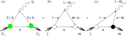
Figure 2: The covariant diagram (a) corresponds to the sum of the LF valence diagram (b) and the nonvalence diagram (c). The large white and black blobs at the meson-quark vertices in (b) and (c) represent the ordinary LF wave function and the non-wave function vertex, respectively.

The covariant diagram in Fig. 2(a) for the transition form factors between pseudoscalar and vector mesons is in general equivalent to the sum of LF valence diagram (b) and the nonvalence diagram (c), where $\alpha=P_{2}^{+}/P_{1}^{+}=1-q^{+}/P_{1}^{+}$. From the covariant diagram of Fig. 2(a), the matrix element $\langle J^{\mu}_{V-A}\rangle_{h}\equiv\langle P_{2};1h|J^{\mu}_{V-A}|P_{1};00\rangle$ is given by

$$\langle J^{\mu}_{V-A}\rangle_{h}=ig_{1}g_{2}\int\frac{d^{4}k}{(2\pi)^{4}}\frac{S_{\Lambda_{1}}(P_{1}-k)S^{\mu}_{h}S_{\Lambda_{2}}(P_{2}-k)}{S_{m_{1}}S_{m}S_{m_{2}}},{}$$ (4)

where $g_{1}$ and $g_{2}$ are the normalization factors which can be fixed by requiring charge form factors of pseudoscalar and vector mesons to be unity at $q^{2}=0$, respectively. Following the previous work BCJ1 , we replaced the point gauge-boson vertex $\gamma^{\mu}(1-\gamma_{5})$ by a non-local(smeared) gauge-boson vertex $S_{\Lambda_{1}}(P_{1}-k)\gamma^{\mu}(1-\gamma_{5})S_{\Lambda_{2}}(P_{2}-k)$ to regularize the covariant fermion triangle loop in ($3+1$) dimensions, where $S_{\Lambda_{i}}(P_{i})=\Lambda^{2}_{i}/(P_{i}^{2}-{\Lambda_{i}}^{2}+i\varepsilon)$ and $\Lambda_{i}$ plays the role of momentum cut-off similar to the Pauli-Villars regularization. The rest of the denominators in Eq. (4) coming from the intermediate fermion propagators in the triangle loop diagram are given by

$$S_{m_{1}} = p_{1}^{2}-{m_{1}}^{2}+i\varepsilon,$$

$$S_{m} = k^{2}-m^{2}+i\varepsilon,$$

$$S_{m_{2}} = p_{2}^{2}-{m_{2}}^{2}+i\varepsilon,{}$$ (5)

where $m_{1}$, $m$, and $m_{2}$ are the masses of the constituents carrying the intermediate four-momenta $p_{1}=P_{1}-k$, $k$, and $p_{2}=P_{2}-k$, respectively.

The trace term in Eq. (4), $S^{\mu}_{h}$, is given by

$$S^{\mu}_{h}={\rm Tr}[(\not\!p_{2}+m_{2})\gamma^{\mu}(1-\gamma_{5})(\not\!p_{1}+m_{1})\gamma_{5}(-\not\!k+m)\epsilon^{*}\cdot\Gamma],{}$$ (6)

where the final state vector meson vertex operator $\Gamma^{\mu}$ is given by

$$\Gamma^{\mu}=\gamma^{\mu}-\frac{(P_{2}-2k)^{\mu}}{D}.$$ (7)

We shall analyze the three different cases of $D$-term,i.e.

$$(1)D_{\rm cov}(M_{V})=M_{V}+m_{2}+m,$$

$$(2)D_{\rm cov}(k\cdot P_{2})=\frac{[2k\cdot P_{2}+M_{V}(m_{2}+m)-i\epsilon]}{M_{V}},$$

$$(3)D_{LF}(M^{\prime}_{0})=M^{\prime}_{0}+m_{2}+m,$$ (8)

where the prime denotes the final state.

In our trace term calculation, we separate Eq. (6) into the on-mass-shell propagating part $S^{\mu}_{\rm on}$ and the off-mass-shell part $S^{\mu}_{\rm off}$,i.e.

$${}S^{\mu}_{h} = (S^{\mu}_{h})_{\rm on}+(S^{\mu}_{h})_{\rm off},$$ (9)

via

$${}\not\!p+m = (\not\!p_{\rm on}+m)+\frac{1}{2}\gamma^{+}(p^{-}-p^{-}_{\rm on}).$$ (10)

While the on-mass-shell part $(S^{\mu}_{h})_{\rm on}$ indicates that all three quarks are on their respective mass-shell,i.e. $k^{-}=k^{-}_{\rm on}$ and $p^{-}_{i}=p^{-}_{i\rm on}(i=1,2)$, the off-mass-shell part $(S^{\mu}_{h})_{\rm off}$ includes the term proportional to $(k^{-}-k^{-}_{\rm on})$ BCJ03 . The trace terms $(S^{+}_{h})_{V}$ and $(S^{+}_{h})_{A}$ in Eq. (6) for the vector and axial-vector currents are given by

$$(S^{+}_{h})_{V} = 4i\varepsilon^{+\mu\nu\alpha}\biggl{[}[m_{1}(p_{2\rm on})_{\mu}(k_{\rm on})_{\nu}-m_{2}(p_{1\rm on})_{\mu}(k_{\rm on})_{\nu}-m(p_{1\rm on})_{\mu}(p_{2\rm on})_{\nu}]\epsilon^{*}_{\alpha}-\frac{(p_{2}-k)\cdot\epsilon^{*}(h)}{D}(p_{1\rm on})_{\mu}(p_{2\rm on})_{\nu}(k_{\rm on})_{\alpha}\biggr{]}$$

$$(S^{+}_{h})_{A} = 4m_{1}[(k_{\rm on}\cdot\epsilon^{*})p^{+}_{2\rm on}+(p_{2\rm on}\cdot\epsilon^{*})k^{+}_{\rm on}-(p_{2\rm on}\cdot k_{\rm on})\epsilon^{*+}]-4m_{2}[(k_{\rm on}\cdot\epsilon^{*})p^{+}_{1\rm on}-(p_{1\rm on}\cdot\epsilon^{*})k^{+}_{\rm on}+(p_{1\rm on}\cdot k_{\rm on})\epsilon^{*+}]$$ (11)

$$+4m[(p_{2\rm on}\cdot\epsilon^{*})p^{+}_{1\rm on}+(p_{1\rm on}\cdot\epsilon^{*})p^{+}_{2\rm on}-(p_{1\rm on}\cdot p_{2\rm on})\epsilon^{*+}]-4m_{1}m_{2}m\epsilon^{*+}-4(k^{-}-k^{-}_{\rm on})m_{2}p^{+}_{1\rm on}\epsilon^{*+}$$

$$+4\frac{(p_{2}-k)\cdot\epsilon^{*}(h)}{D}\biggl{[}(p_{2\rm on}\cdot k_{\rm on}-m_{2}m)p^{+}_{1}+(p_{1\rm on}\cdot k_{\rm on}+m_{1}m)p^{+}_{2}-(p_{1\rm on}\cdot p_{2\rm on}+m_{1}m_{2})k^{+}$$

$$\hskip 85.35826pt+(k^{-}-k^{-}_{\rm on})p^{+}_{1\rm on}p^{+}_{2\rm on}\biggr{]}.$$

A different approach calculating Eq. (6) can be found in Refs Ja99 ; Ja03 where Jaus used the four-vector and tensor decompositions of the internal four-momentum $p_{1}$ including the lightlike four-vector $\omega$ in the trace terms,e.g. four-vector decomposition of $p_{1}$ is given by $p_{1\mu}=A^{(1)}_{1}P_{\mu}+A^{(1)}_{2}q_{\mu}+C^{(1)}_{1}\omega_{\mu}$, where $C$-type functions are $\omega$-dependent while $A$-type functions are $\omega$-independent. His main idea for the calculation of the trace term is to separate the term proportional to $N_{2}=k^{2}-m^{2}$ from the rest of the terms in the trace. The $\omega$-dependent $C$-type(and also $B$-type arising from the tensor decomposition of $p_{1\mu}p_{1\nu}$) functions include this $N_{2}$-term, e.g. $C^{(1)}_{1}=-N_{2}+Z_{2}(x,{\bf k}_{\perp})$. Although this $N_{2}$-term vanishes for the spectator quark with the momentum $k$ being on-mass-shell($k^{-}=k^{-}_{\rm on}$), it may give nonvanishing contribution if the spectator quark is off-mass-shell, i.e. $k^{-}=p^{-}_{1\rm on}$. If this happens, then the nonvanishing $N_{2}$-term contribution related to the zero-mode contribution should be included to obtain the Lorentz invariant form factor. Jaus discussed that the inclusion of the zero-mode(without involving higher Fock states or the nonvalence contributions) can be made by the replacement $N_{2}\to Z_{2}$,i.e. $C^{(1)}\doteq 0$. However, his $C^{(1)}\doteq 0$ prescription is valid only at the particular choice of the vector meson vertex operator $\Gamma^{\mu}$ in Eq. (7),e.g. $C^{(1)}\doteq 0$ is valid only for the $D_{\rm cov}(M_{V})$ in Eq. (II) but not for $D_{\rm cov}(k\cdot P_{2})$ and $D_{LF}(M^{\prime}_{0})$ as we shall show in the following sections. For the comparison with Jaus’s $N_{2}$-term prescription later on, we note that his $N_{2}$-term corresponds to our $(k^{-}-k^{-}_{\rm on})$-term via $N_{2}=k^{2}-m^{2}=k^{+}(k^{-}-k^{-}_{\rm on})+k^{2}_{\rm on}-m^{2}=k^{+}(k^{-}-k^{-}_{\rm on})$.

III Light-front calculation of the weak form factors

In the LF calculation of the weak form factors, we use ${\bf P}_{1\perp}=0$ frame with the (timelike) momentum transfer $q^{2}=(P_{1}-P_{2})^{2}$ given by

$${}q^{2}=q^{+}q^{-}-{\bf q}^{2}_{\perp}=(1-\alpha)\biggl{(}M^{2}_{1}-\frac{M^{2}_{2}}{\alpha}\biggr{)}-\frac{{\bf q}^{2}_{\perp}}{\alpha}.$$ (12)

We shall use only the plus component of the $V-A$ current for the calculations of LF valence[Fig. 2(b)] and nonvalence [Fig. 2(c)] diagrams.

III.1 Matrix elements of the weak current

In the valence region $0<k^{+}<P^{+}_{2}$, the pole $k^{-}=k^{-}_{\rm on}=(m^{2}+{\bf k}^{2}_{\perp}-i\varepsilon)/k^{+}$ (i.e., the spectator quark) is located in the lower half of the complex $k^{-}$-plane.

Thus, the Cauchy formula for the $k^{-}$-integration in Eq. (4) gives

$${}\langle J^{+}_{V-A}\rangle^{h}_{\rm val} = \frac{g_{1}g_{2}\Lambda^{2}_{1}\Lambda^{2}_{2}}{2(2\pi)^{3}}\int^{\alpha}_{0}\frac{dx}{x}\int d^{2}{\bf k}_{\perp}$$ (13)

$$\times\psi_{i}(x,{\bf k}_{\perp})(S^{+}_{h})_{\rm on}\psi_{f}(x^{\prime},{\bf k^{\prime}}_{\perp}),$$

where

$$\psi_{i}(x,{\bf k}_{\perp}) = \frac{1}{(1-x)^{2}(M^{2}_{1}-M^{2}_{0})(M^{2}_{1}-M^{2}_{\Lambda_{1}})},$$

$$\psi_{f}(x^{\prime},{\bf k^{\prime}}_{\perp}) = \frac{1}{(1-x^{\prime})^{2}(M^{2}_{2}-M^{\prime 2}_{0})(M^{2}_{2}-M^{\prime 2}_{\Lambda_{2}})},$$

and

$$M^{2}_{0} = \frac{{\bf k}^{2}_{\perp}+m^{2}_{1}}{1-x}+\frac{{\bf k}^{2}_{\perp}+m^{2}}{x},$$

$$M^{\prime 2}_{0} = \frac{{\bf k^{\prime}}^{2}_{\perp}+m^{2}_{2}}{1-x^{\prime}}+\frac{{\bf k^{\prime}}^{2}_{\perp}+m^{2}}{x^{\prime}},$$

$$M^{2}_{\Lambda_{1}} = M^{2}_{0}(m_{1}\to\Lambda_{1}),\;M^{\prime 2}_{\Lambda_{2}}=M^{\prime 2}_{0}(m_{2}\to\Lambda_{2}).$$ (15)

The final state momentum variables are given by ${\bf k^{\prime}}_{\perp}={\bf k}_{\perp}+x^{\prime}{\bf q}_{\perp}$ and $x^{\prime}=x/\alpha$. Note that the trace term in Eq. (13) includes only the on-mass-shell propagating part since the pole structure $k^{-}=k^{-}_{\rm on}$(or equivalently $N_{2}=0$) leads to the vanishing off-mass-shell contributions.

In the nonvalence region $P^{+}_{2}<k^{+}<P^{+}_{1}$, the poles at $k^{-}=k^{-}_{m_{1}}\equiv P^{-}_{1}+[m^{2}_{1}+({\bf k}_{\perp}-{\bf P}_{1\perp})^{2}-i\varepsilon]/(k^{+}-P^{+}_{1})$ (from the struck quark propagator) and $k^{-}=k^{-}_{\Lambda_{1}}\equiv P^{-}_{1}+[\Lambda^{2}_{1}+({\bf k}_{\perp}-{\bf P}_{1\perp})^{2}-i\varepsilon]/(k^{+}-P^{+}_{1})$ (from the smeared quark-photon vertex), are located in the upper half of the complex $k^{-}$-plane.

Thus, the Cauchy integration over $k^{-}$ in Eq. (4) gives

$$\langle J^{+}_{V-A}\rangle^{h}_{\rm nv}$$

$$=\frac{g_{1}g_{2}\Lambda^{2}_{1}\Lambda^{2}_{2}}{2(2\pi)^{3}(\Lambda^{2}_{1}-m^{2}_{1})}\int^{1}_{\alpha}\frac{dx}{xx^{\prime\prime}(1-x^{\prime\prime})(x-\alpha)}$$

$$\times\int d^{2}{\bf k}_{\perp}\biggl{\{}\frac{S^{+}_{h}(k^{-}_{\Lambda_{1}})}{(M^{2}_{1}-M^{2}_{\Lambda_{1}})(q^{2}-M^{2}_{\Lambda_{1}\Lambda_{2}})(q^{2}-M^{2}_{\Lambda_{1}m_{2}})}$$

$$\;\;\;\;-\frac{S^{+}_{h}(k^{-}_{m_{1}})}{(M^{2}_{1}-M^{2}_{0})(q^{2}-M^{2}_{m_{1}\Lambda_{2}})(q^{2}-M^{2}_{m_{1}m_{2}}))}\biggr{\}},$$ (16)

where

$$M^{2}_{\Lambda_{1}\Lambda_{2}} = \frac{{\bf k^{\prime\prime}}^{2}_{\perp}+\Lambda^{2}_{1}}{x^{\prime\prime}}+\frac{{\bf k^{\prime\prime}}^{2}_{\perp}+\Lambda^{2}_{2}}{1-x^{\prime\prime}},$$

$$M^{2}_{\Lambda_{1}m_{2}} = \frac{{\bf k^{\prime\prime}}^{2}_{\perp}+\Lambda^{2}_{1}}{x^{\prime\prime}}+\frac{{\bf k^{\prime\prime}}^{2}_{\perp}+m^{2}_{2}}{1-x^{\prime\prime}},$$

$$M^{2}_{m_{1}m_{2}} = \frac{{\bf k^{\prime\prime}}^{2}_{\perp}+m^{2}_{1}}{x^{\prime\prime}}+\frac{{\bf k^{\prime\prime}}^{2}_{\perp}+m^{2}_{2}}{1-x^{\prime\prime}},$$

$$M^{2}_{m_{1}\Lambda_{2}} = \frac{{\bf k^{\prime\prime}}^{2}_{\perp}+m^{2}_{1}}{x^{\prime\prime}}+\frac{{\bf k^{\prime\prime}}^{2}_{\perp}+\Lambda^{2}_{2}}{1-x^{\prime\prime}},$$ (17)

and

$$x^{\prime\prime} = \frac{1-x}{1-\alpha},\;{\bf k^{\prime\prime}}_{\perp}={\bf k}_{\perp}+x^{\prime\prime}{\bf q}_{\perp}.$$ (18)

The explicit forms of the trace terms $S^{+}_{h}(k^{-}_{m_{1}})$ and $S^{+}_{h}(k^{-}_{\Lambda_{1}})$ are given in the Appendix. In general, the trace terms in the nonvalence diagram include the off-mass-shell contributions(or equivalently $N_{2}\neq 0$),e.g. $S^{+}_{h}(k^{-}_{m_{1}})=(S^{+}_{h})_{\rm on}+(S^{+}_{h})_{\rm off}(k^{-}_{m_{1}})$.

III.2 Extraction of weak form factors

From Eqs. (2), (II) and (12), one obtains the relations between the current matrix elements and the weak form factors as follows

$${}\langle J^{+}_{V}\rangle^{h=1} = -\frac{P^{+}_{1}}{\sqrt{2}}\varepsilon^{+-xy}q^{L}g(q^{2}),$$

$$\langle J^{+}_{V}\rangle^{h=0} = 0,$$ (19)

for the vector current and

$${}\langle J^{+}_{A}\rangle^{h=1} = \frac{P^{+}_{1}q^{L}}{\alpha\sqrt{2}}\biggl{[}(1+\alpha)a_{+}(q^{2})+(1-\alpha)a_{-}(q^{2})\biggr{]},$$

$$\langle J^{+}_{A}\rangle^{h=0} = \frac{\alpha P^{+}_{1}}{M_{2}}f(q^{2})+\frac{\alpha P^{+}_{1}}{2M_{2}}\biggl{(}M^{2}_{1}-\frac{M^{2}_{2}}{\alpha^{2}}+\frac{{\bf q}^{2}_{\perp}}{\alpha^{2}}\biggr{)}$$ (20)

$$\times \biggl{[}(1+\alpha)a_{+}(q^{2})+(1-\alpha)a_{-}(q^{2})\biggr{]},$$

for the axial-vector current. Here, $q^{L}=q_{x}-iq_{y}$.

The extraction of weak form factors can be made in various ways. Among them, there are two popular ways of extracting the form factors, e.g. one can obtain the form factors (1) in the spacelike region using the $q^{+}=0$ frame and then analytically continue to the timelike region by changing ${\bf q}_{\perp}$ to $i{\bf q}_{\perp}$ in the form factor, or (2) in a direct timelike region using a $q^{+}>0$ frame.

In this work, we shall use both the $q^{+}=0$ frame ($q^{2}=-{\bf q}^{2}_{\perp}$) and the purely longitudinal momentum frame ($q^{+}>0$ and ${\bf q}_{\perp}=0$) where

$${}q^{2} = q^{+}q^{-}=(1-\alpha)\biggl{(}M^{2}_{1}-\frac{M^{2}_{2}}{\alpha}\biggr{)}.$$ (21)

For this particular choice of the purely longitudinal momentum frame, there are two solutions of $\alpha$ for a given $q^{2}$,i.e.

$${}\alpha_{\pm}=\frac{M_{2}}{M_{1}}\biggl{[}\frac{M^{2}_{1}+M^{2}_{2}-q^{2}}{2M_{1}M_{2}}\pm\sqrt{\biggl{(}\frac{M^{2}_{1}+M^{2}_{2}-q^{2}}{2M_{1}M_{2}}\biggr{)}^{2}-1}\biggr{]},$$ (22)

where the $+(-)$ sign in Eq. (22) corresponds to the daugther meson recoiling in the positive(negative) $z$-direction relative to the parent meson. At the zero recoil ($q^{2}=q^{2}_{\rm max}$) and the maximum recoil ($q^{2}=0$), $\alpha_{\pm}$ are respectively given by

$${}\alpha_{+}(q^{2}_{\rm max}) = \alpha_{-}(q^{2}_{\rm max})=\frac{M_{2}}{M_{1}},$$

$$\alpha_{+}(0) = 1,\;\;\alpha_{-}(0)=\biggl{(}\frac{M_{2}}{M_{1}}\biggr{)}^{2}.$$ (23)

The form factors should in principle be independent of the recoil directions ($\alpha_{\pm}$) if the nonvalence contributions are added to the valence ones.

While the form factor $g(q^{2})$ in the $q^{+}>0$ frame can be obtained directly from Eq. (III.2), the form factor $f(q^{2})$ can be obtained only after $a_{\pm}(q^{2})$ are calculated. To illustrate this, we define

$${}\langle J^{+}_{A}\rangle^{h=1}|_{\alpha=\alpha_{\pm}} \equiv \frac{P^{+}_{1}q^{L}}{\sqrt{2}}I^{+}_{A}(\alpha_{\pm}).$$ (24)

Then we obtain from Eq. (III.2)

$${}a_{+}(q^{2}) = \frac{\alpha_{+}(1-\alpha_{-})I^{+}_{A}(\alpha_{+})-\alpha_{-}(1-\alpha_{+})I^{+}_{A}(\alpha_{-})}{2(\alpha_{+}-\alpha_{-})},$$

$$a_{-}(q^{2}) = -\frac{\alpha_{+}(1+\alpha_{-})I^{+}_{A}(\alpha_{+})-\alpha_{-}(1+\alpha_{+})I^{+}_{A}(\alpha_{-})}{2(\alpha_{+}-\alpha_{-})},$$

and

$${}f(q^{2}) = \frac{M_{2}}{\alpha P^{+}_{1}}\langle J^{+}_{A}\rangle^{h=0}-\frac{1}{2}\biggl{(}M^{2}_{1}-\frac{M^{2}_{2}}{\alpha^{2}}\biggr{)}$$ (26)

$$\times\biggl{[}(1+\alpha)a_{+}(q^{2})+(1-\alpha)a_{-}(q^{2})\biggr{]}.$$

As can be seen from Eqs. (III.2) and (III.2), one should be careful in setting ${\bf q}_{\perp}=0$ to get the correct results in the purely longitudinal frame. One cannot simply set ${\bf q}_{\perp}=0$ from the start, but should set it to zero only after the form factors are extracted.

In the $q^{+}>0$ frame where ${\bf q}_{\perp}\neq 0$, the valence contribution to $g(q^{2})$ is given by

$$g_{\rm val}(q^{2}) = \frac{N}{8\pi^{3}}\int^{\alpha}_{0}\frac{dx}{x}\int d^{2}{\bf k}_{\perp}\;\psi_{i}\psi_{f}\biggl{\{}{\cal A}_{p}+\frac{{\bf k}_{\perp}\cdot{\bf q}_{\perp}}{{\bf q}^{2}_{\perp}}[\alpha(m_{1}-m)+(m-m_{2})]+\frac{2}{D}\biggl{[}{\bf k}^{2}_{\perp}-\frac{({\bf k}_{\perp}\cdot{\bf q}_{\perp})^{2}}{{\bf q}^{2}_{\perp}}\biggr{]}\biggr{\}},$$ (27)

where $N=g_{1}g_{2}\Lambda^{2}_{1}\Lambda^{2}_{2}$ and ${\cal A}_{p}=xm_{1}+(1-x)m$. The form factor $g^{DY}(q^{2})$ in $q^{+}=0$ (or Drell-Yan(DY)) frame is given by

$$g^{DY}(q^{2})=\lim_{\alpha\to 1}g_{\rm val}(q^{2}).$$ (28)

Our result for $g^{DY}(q^{2})$ is the same as the one obtained by Jaus(see Eq. (4.13) in Ja99 ). Note that one needs to replace $x$ by $(1-x)$ and ${\bf q}_{\perp}$ by $-{\bf q}_{\perp}$ between the two formulations to compare each other directly. The form factor $g(q^{2})$ is found to be free from the zero-mode contribution. The nonvalence contribution to $g(q^{2})$ in $q^{+}>0$ frame can be obtained from Eq. (LABEL:jnv) with the trace term given by Eq. (36).

The valence contribution to the matrix elements $I^{+}_{A}(\alpha)$ for $a_{\pm}(\alpha)$ in Eq. (III.2) is given by

$$(I^{+}_{A})_{\rm val}(\alpha) = \frac{2N}{8\pi^{3}}\int^{\alpha}_{0}\frac{dx}{x}\int d^{2}{\bf k}_{\perp}\;\psi_{i}\psi_{f}\biggl{\{}(1-2x^{\prime}){\cal A}_{p}+\frac{{\bf k}_{\perp}\cdot{\bf q}_{\perp}}{{\bf q}^{2}_{\perp}}[(\alpha-2x)(m_{1}-m)-(m_{2}+m)]$$ (29)

$$\hskip 28.45274pt-\frac{2}{x^{\prime}D}\biggl{(}x^{\prime}+\frac{{\bf k}_{\perp}\cdot{\bf q}_{\perp}}{{\bf q}^{2}_{\perp}}\biggr{)}\biggl{(}{\bf k}_{\perp}\cdot{\bf k^{\prime}}_{\perp}+{\cal A}_{p}[(1-x^{\prime})m-x^{\prime}m_{2}]\biggr{)}\biggr{\}}.$$

The form factor $a^{DY}_{+}(q^{2})$ in $q^{+}=0$ frame is given by

$$a^{DY}_{+}(q^{2})=\lim_{\alpha\to 1}\frac{(I^{+}_{A})_{\rm val}(\alpha)}{2}.$$ (30)

Our result of $a^{DY}_{+}(q^{2})$ is the same as the one obtained by Jaus(see Eq. (4.14) in Ja99 ). The form factor $a_{+}(q^{2})$ is also found to be free from the zero-mode contribution. The nonvalence contribution to $a_{+}(q^{2})$ in $q^{+}>0$ frame can be obtained from Eq. (LABEL:jnv) with the trace term given by Eq. (37).

To obtain the form factor $f(q^{2})$ in Eq. (26), we need to compute the matrix element involving the helicity zero,i.e. $\langle J^{+}_{A}\rangle^{h=0}$. The explicit form of the valence contribution to $\langle J^{+}_{A}\rangle^{h=0}$ is given by

$$\langle J^{+}_{A}\rangle^{h=0}_{\rm val} = -\frac{2N}{8\pi^{3}}\frac{P^{+}_{1}}{M_{2}}\int^{\alpha}_{0}\frac{dx}{xx^{\prime}}\int\;d^{2}{\bf k}_{\perp}\;\psi_{i}\psi_{f}\biggl{\{}{\cal A}_{p}[x^{\prime}(1-x^{\prime})M^{2}_{2}+m_{2}m+x^{\prime 2}{\bf q}^{2}_{\perp}]+{\bf k}^{2}_{\perp}(xm_{1}+m_{2}-xm)$$ (31)

$$+x^{\prime}{\bf k}_{\perp}\cdot{\bf q}_{\perp}[2x(m_{1}-m)+m_{2}+m]-\frac{(x^{\prime 2}M^{2}_{2}-{\bf k^{\prime}}^{2}_{\perp}-m^{2})}{D}\biggl{(}{\bf k}_{\perp}\cdot{\bf k^{\prime}}_{\perp}+{\cal A}_{p}[(1-x^{\prime})m-x^{\prime}m_{2}]\biggr{)}\biggr{\}}.$$

The form factor $f^{DY}(q^{2})$ in $q^{+}=0$ frame obtained from Eq. (III.2),i.e.

$${}f^{DY}(q^{2})=-(M^{2}_{1}-M^{2}_{2}+{\bf q}^{2}_{\perp})a^{DY}_{+}(q^{2})+\frac{M_{2}}{P^{+}_{1}}\lim_{\alpha\to 1}\langle J^{+}_{A}\rangle^{h=0}_{\rm val},$$ (32)

is explicitly given by

$$f^{DY}(q^{2}) = -\frac{N}{8\pi^{3}}\int^{1}_{0}\frac{dx}{x^{2}}\int\;d^{2}{\bf k}_{\perp}\;\psi_{i}\psi_{f}\biggl{\{}2{\bf k}^{2}_{\perp}(xm_{1}+m_{2}-xm)+2x{\bf k}_{\perp}\cdot{\bf q}_{\perp}[2x(m_{1}-m)+m_{2}+m]$$ (33)

$$\;+{\cal A}_{p}[x(1-2x)M^{2}_{1}+xM^{2}_{2}+2m_{2}m+x{\bf q}^{2}_{\perp}]+x[q\cdot P+{\bf q}^{2}_{\perp}][(1-2x)(m_{1}-m)-m_{2}-m]\frac{{\bf k}_{\perp}\cdot{\bf q}_{\perp}}{{\bf q}^{2}_{\perp}}$$

$$\;-\frac{2}{xD}\biggl{(}{\bf k}_{\perp}\cdot{\bf k}^{\prime}_{\perp}+{\cal A}_{p}[(1-x)m-xm_{2}]\biggr{)}\biggl{(}x[q\cdot P+{\bf q}^{2}_{\perp}][x+\frac{{\bf k}_{\perp}\cdot{\bf q}_{\perp}}{{\bf q}^{2}_{\perp}}]+x^{2}M^{2}_{2}-{\bf k}^{\prime 2}_{\perp}-m^{2}\biggr{)}\biggr{\}},$$

where $q\cdot P=M^{2}_{1}-M^{2}_{2}$. We should note that our result for $\lim_{\alpha\to 1}\langle J^{+}_{A}\rangle^{h=0}_{\rm val}$(i.e. $f^{DY}(q^{2})$) is different from the result obtained by the LF formalism discussed in the Appendix C of Ref.Ja03 (see,e.g. Eq. (C2) in Ja03 ). That formalismJa03 requires all quarks to be on their respective mass-shells and replaces the physical vector meson mass $M_{2}$ in Eq. (II) by the invariant meson mass $M^{\prime}_{0}$. However, our result is obtained by requiring only the struck quark($m_{2}$) to be on-mass-shell and using the physical vector meson mass $M_{2}$ in Eq. (II). The nonvalence contribution to $\langle J^{+}_{A}\rangle^{h=0}$ in $q^{+}>0$ frame can be obtained from Eq. (LABEL:jnv) with the trace term given by Eq. (A) in our Appendix.

We now determine whether $f(q^{2})$,i.e. $f^{DY}(q^{2})$, is free from the zero-mode. The zero-mode contribution to $\langle J^{+}_{A}\rangle^{h}$ is defined as

$$\langle J^{+}_{A}\rangle^{h}_{\rm z.m.}=\lim_{\alpha\to 1}\langle J^{+}_{A}\rangle^{h}_{\rm nv}.$$ (34)

To check if the zero-mode exists or not, we use the counting rule for the factors of the longitudinal momentum fraction in Eq. (LABEL:jnv),e.g. in the $q^{+}\to 0$ limit, the first term in Eq. (LABEL:jnv) becomes

$${}\langle J^{+}_{A}\rangle^{h}_{\rm z.m.} \sim \lim_{\alpha\to 1}\int^{1}_{\alpha}dx\frac{x(1-x)[x^{\prime\prime}(1-x^{\prime\prime})]^{2}}{xx^{\prime\prime}(1-x^{\prime\prime})(x-\alpha)}S^{+}_{h}(k^{-}_{\Lambda_{1}})[\cdots]$$ (35)

$$= \lim_{\alpha\to 1}\int^{1}_{\alpha}dx\frac{(1-x)^{2}}{(1-\alpha)^{2}}S^{+}_{h}(k^{-}_{\Lambda_{1}})[\cdots]$$

$$= \lim_{\alpha\to 1}\int^{1}_{0}dz(1-\alpha)(1-z)^{2}S^{+}_{h}(k^{-}_{\Lambda_{1}})[\cdots],$$

where the variable change $x=\alpha+(1-\alpha)z$ was made and the terms in $[\cdots]$ are regular in the $\alpha\to 1$(or equivalently $x\to 1$) limit. The second term in Eq. (LABEL:jnv) with $S^{+}_{h}(k^{-}_{m_{1}})$ has the same power counting of the longitudinal momentum fraction as the first term in Eq. (35).

From Eq. (35), one can determine the existence/non-existence of the zero-mode contribution to $f^{DY}(q^{2})$ by counting the factors of the longitudinal momentum fraction, specifically $(1-x)$-factors, in the trace terms $S^{+}_{h=0}(k^{-}_{\Lambda_{1}})$ and $S^{+}_{h=0}(k^{-}_{m_{1}})$. Note that both $k^{-}_{\Lambda_{1}}=k^{-}_{m_{1}}\sim p^{-}_{1\rm on}\sim 1/(1-x)$. Thus, from $(S^{+}_{h=0})_{A}$ in Eq. (II), the terms such as $(k^{-}-k^{-}_{\rm on})p^{+}_{1\rm on}$ are regular for the factor $(1-x)$. All other on-mass-shell terms are also regular for the same factor $(1-x)$. Thus, the only zero-mode suspected term is $(p_{2}-k)\cdot\epsilon^{*}(h=0)/D\sim 1/(1-x)D$.

The power counting of $(1-x)$ in $(S^{+}_{h=0})(k^{-}_{\Lambda_{1}})$ depends on the vector meson vertices (See Eq. (II)). We find that $(S^{+}_{h=0})(k^{-}_{\Lambda_{1}})$ is proportional to (1) $(1-x)^{-1}=[(1-\alpha)(1-z)]^{-1}$ for $D_{\rm cov}(M_{V})$, (2) $(1-x)^{0}$ for $D_{\rm cov}(k\cdot P_{2})$, and (3) $(1-x)^{-1/2}=[(1-\alpha)(1-z)]^{-1/2}$ for $D_{LF}(M^{\prime}_{0})$, respectively. These power-counting results show that the form factor $f^{DY}(q^{2})$ receives the zero-mode contribution only for the $D_{\rm cov}(M_{V})$ case but not for others. In fact, our power-counting should also hold in Jaus’s case,i.e. $N_{2}/D$ for the zero-mode limit goes to (1) $Z_{2}/D$ for $D_{\rm cov}(M_{V})$, (2) $(1-x)N_{2}\doteq 0$ for $D_{\rm cov}(k\cdot P_{2})$, and (3) $\sqrt{(1-x)}N_{2}\doteq 0$ for $D_{LF}(M^{\prime}_{0})$, respectively. On the other hand, Jaus Ja03 ; Ja99 used $N_{2}/D\doteq Z_{2}/D$ regardless of the $D$-terms and removed $C$-type functions as well as $B$-type functions. This explains how he reached the conclusion that the form factor $f(q^{2})$ receives the zero-mode contribution regardless of the vertices used in the model calculation. We have shown that his conclusion is correct for the case (1) (or $D_{\rm cov}(M_{V})$) but not for the cases (2)(or $D_{\rm cov}(k\cdot P_{2})$) and (3)(or $D_{LF}(M^{\prime}_{0})$). We now confirm our derivation through the numerical calculation in the next section.

IV Numerical results

In this section, we present the numerical results for the $B\to\rho$ transition form factors ($g(q^{2}),a_{+}(q^{2}),f(q^{2})$) in the three different cases of meson vertex discussed above. We perform our LF calculation in the two different reference frames, i.e. $q^{+}=0$ and purely longitudinal $q^{+}>0$ frames. We also compare our results with those obtained by Jaus Ja99 ; Ja03 . We do not aim at finding the best-fit parameters to describe the experimental data in this work. However, the essential findings from the generic structure of our model calculations are expected to apply also for the more realistic models, although the quantitative results would depend on the details of the model. The model parameters for $B$ and $\rho$ mesons are taken same as in Ref.BCJ03 : $M_{B}=5.28$ GeV, $M_{\rho}=0.771$ GeV, $m_{b}=4.9$ GeV, $\Lambda_{b}=10$ GeV, and $g_{B}=5.20$, as well as $m_{u}=m_{d}=0.43$ GeV, $\Lambda_{u(d)}=1.5$ GeV, and $g_{\rho}=5.13$.

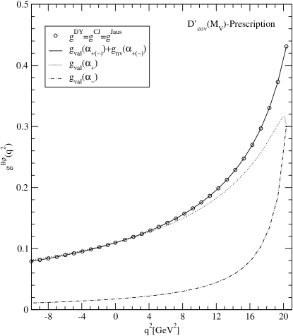
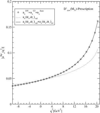
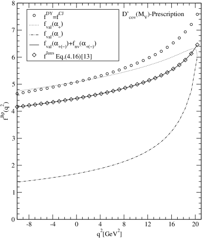
Figure 3: Weak form factors $g(q^{2}),a_{+}(q^{2})$ and $f(q^{2})$ for $B\to\rho$ transition obtained from the case of the vector meson vertex with $D_{\rm cov}(M_{V})=M_{V}+m_{2}+m$.

In Fig. 3, we present the weak form factors $g(q^{2}),a_{+}(q^{2})$ and $f(q^{2})$ for $B\to\rho$ transition obtained in the case of $D_{\rm cov}(M_{V})=M_{V}+m_{2}+m$,i.e. the case (1). The white circle represents the result in the $q^{+}=0$ frame obtained by the analytic continuation from spacelike to timelike $q^{2}$ region. We denote these form factors as $g^{\rm CJ}(q^{2}),a_{+}^{\rm CJ}(q^{2})$ and $f^{\rm CJ}(q^{2})$. For the case of $g$ form factor, we can present seperately $\alpha_{+}$ and $\alpha_{-}$ results for the valence contribution since the valence calculation in the purely longitudinal frame can be done either by $\alpha_{+}$ or by $\alpha_{-}$ independently. However, this is not the case for $a_{+}$ form factor as shown in Eq. (III.2). Thus, we do not separate the $\alpha_{+}$ result from $\alpha_{-}$ result for the form factor $a_{+}(q^{2})$. For the form factor $g(q^{2})$, the dotted and dot-dashed lines represent the valence results obtained in the purely longitudinal $q^{+}>0$ frame with $\alpha_{+}$ and $\alpha_{-}$, respectively. The solid line represents the full(=valence + nonvalence) result obtained from the purely longitudinal $q^{+}>0$ frame. As expected, the full result in $q^{+}>0$ frame is $\alpha_{+}$ and $\alpha_{-}$ independent. For the form factor $a_{+}(q^{2})$, the valence and full results are shown by the dotted and solid lines, respectively. In Fig. 3, we have also compared our results with the ones obtained from Jaus’s Eqs. (4.13), (4.14) and (4.16) in Ref. Ja99 for the form factors $g(q^{2}),a_{+}(q^{2})$, and $f(q^{2})$, respectively. For the form factors $g(q^{2})$ and $a_{+}(q^{2})$, our results from $q^{+}=0$ frame, i.e. $g^{\rm CJ}(q^{2})$ and $a^{\rm CJ}_{+}(q^{2})$, are equivalent to Jaus’s results of $g^{\rm Jaus}(q^{2})$ and $a^{\rm Jaus}_{+}(q^{2})$ since they do not include $B$ and $C$-type functions in the LF integral. Our results from $q^{+}=0$ frame are also in exact agreement with the full(valence + nonvalence) solutions obtained in the purely longitudinal $q^{+}>0$ frame. This shows that our full results of $g(q^{2})$ and $a_{+}(q^{2})$ are not only Lorentz invariant but also immune to the zero-mode contribution. For the form factor $f(q^{2})$, however, our result $f^{\rm CJ}(q^{2})$ in $q^{+}=0$ frame shows the existence of the zero-mode as explained by the counting rule in Sec.III. The zero-mode contribution to $f^{\rm CJ}(q^{2})$,i.e. the difference between the full solution(solid line) in $q^{+}>0$ frame and $f^{\rm CJ}(q^{2})$ in $q^{+}=0$ frame, is as large as 19$\%$ in the case (1). The zero-mode contribution to $f^{DY}(q^{2})$ in $q^{+}=0$ frame is distinguished from that appears in the purely longitudial $q^{2}=q^{+}q^{-}$ frame. In the purely longitudinal frame, the zero-mode contribution is a single point at $q^{2}=0$ as $q^{+}\to 0$(or equivalently $\alpha_{+}\to 1$), which can be quantified by the difference between $f_{\rm full}=f_{\rm val}(\alpha_{+})+f_{\rm nv}(\alpha_{+})$(solid line) and $f_{\rm val}(\alpha_{+})$(dotted line) at $q^{2}=0$,i.e. $f^{\rm z.m.}(0)=\lim_{\alpha_{+}\to 1}f_{\rm nv}(\alpha_{+})$. We thus distinguish the zero-mode contribution at $q^{+}=0$ from the usual nonvalence one at $q^{-}=0$(or equivalently $\alpha_{-}(0)$) CJ98 . Interestingly, however, Jaus’s result(diamond) is exactly the same as ours in $q^{+}>0$ frame. This indicates that his method of including the zero-mode contribution to $f(q^{2})$ is valid in the case (1)(or $D_{\rm cov}(M_{V})$) as we have discussed in the previous section using our power-counting method.

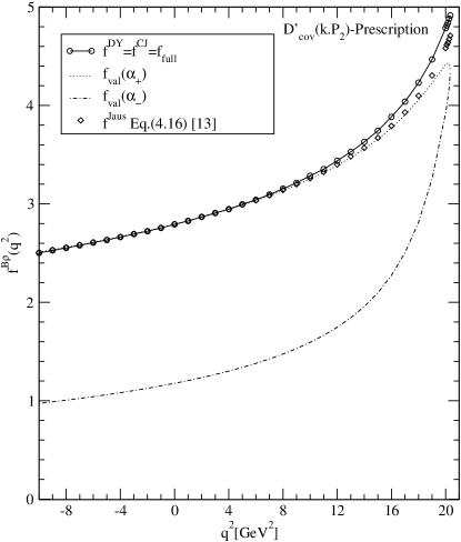
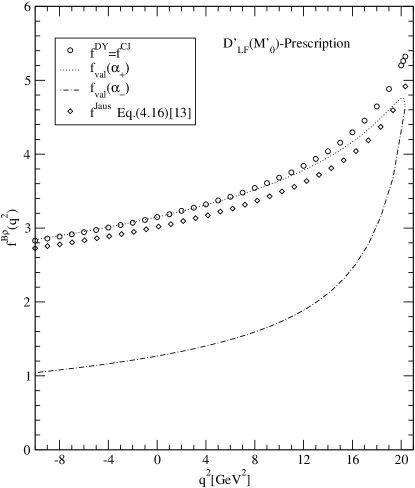
Figure 4: Weak form factor $f(q^{2})$ for $B\to\rho$ transition in the cases of the vector meson vertex with $D_{\rm cov}(k\cdot P_{2})$(left) and $D_{LF}(M^{\prime}_{0})$(right).

In Fig. 4, we present the form factor $f(q^{2})$ for $B\to\rho$ transition in the cases (2)(or $D_{\rm cov}(k\cdot P_{2})$(left)) and (3)(or $D_{LF}(M^{\prime}_{0})$(right)). For the manifestly covariant case (2), our result $f^{\rm CJ}(q^{2})$(circle) obtained in the $q^{+}=0$ frame is in an exact agreement with the full result(solid line) in the purely longitudinal $q^{+}>0$ frame. This shows that there is no zero-mode contribution to $f^{\rm CJ}(q^{2})$ for the vertex with $D_{\rm cov}(k\cdot P_{2})$. The difference between the full result and $f_{\rm val}(\alpha_{+})$(dotted line) or $f_{\rm val}(\alpha_{-})$(dot-dashed line) is not the zero-mode contribution but the nonvalence contribution as described in Fig. 3. Comparing Jaus’s result with ours, we find that $f^{\rm CJ}(q^{2})$ and $f^{\rm Jaus}(q^{2})$ coincide each other at $q^{2}=0$ but differ about $4\%$ at $q=q_{\rm max}$. This difference between Jaus’s and ours is caused by the different treatment of $N_{2}/D$ term as we have illustrated in the previous section(Sec.III). Now, in the case (3) with $D_{LF}(M^{\prime}_{0})$, we compared the result $f^{\rm CJ}(q^{2})$(circle) in the $q^{+}=0$ frame with the valence results obtained in the purely longitudinal $q^{+}>0$ frame with $\alpha_{+}$(dotted line) and $\alpha_{-}$(dot-dashed line), respectively. As we discussed in the previous section using the power-counting rule, the result $f^{\rm CJ}(q^{2})$ without the zero-mode contribution must be identical to the full result. Thus, the differences between $f^{\rm CJ}(q^{2})$ and the valence results(dotted line and dot-dashed line) in the $q^{+}>0$ frame exhibit the nonvalence contributions with $\alpha_{+}$ and $\alpha_{-}$, respectively. Also, the comparison between our full result($f^{\rm CJ}$) and Jaus’s result(diamond) indicate the more substantial(even at $q^{2}=0$) difference due to the different treatment of $N_{2}/D$ term in the case (3) than in the manifestly covariant case (2). For both cases of $D_{LF}(M^{\prime}_{0})$ and $D_{\rm cov}(k\cdot P_{2})$, we have confirmed that the two results(Jaus and CJ) exactly coincide if and only if we set $N_{2}/D\doteq 0$ in Jaus’s formulation.

V Conclusion

In this work, we have analyzed the zero-mode contribution to the weak transition form factors, in particular $f(q^{2})$, between pseudoscalar and vector mesons. For the phenomenologically accessible vector meson vertex $\Gamma^{\mu}=\gamma^{\mu}-(P_{2}-2k)^{\mu}/D$, we discussed the three typical cases of the $D$-term which may be also classified by the differences in the power-counting of the LF energy $k^{-}$,i.e.: (1) $D_{\rm cov}(M_{V})=M_{V}+m_{2}+m\sim(k^{-})^{0}$, (2) $D_{\rm cov}(k\cdot P_{2})=[2k\cdot P_{2}+(m_{2}+m)M_{V}-i\epsilon]/M_{V}\sim(k^{-})^{1}$, and (3) $D_{LF}(M^{\prime}_{0})=M^{\prime}_{0}+m_{2}+m\sim(k^{-})^{1/2}$. Our main idea to obtain the weak transition form factors is first to find if the zero-mode contribution exists or not for the given form factor using the power-counting method. If exists, then the separation of the on-mass-shell propagating part from the off-mass-shell part is useful since the off-mass-shell part is responsible for the zero-mode contribution. We found that the form factors $g(q^{2})$ and $a_{+}(q^{2})$ are immune to the zero-mode contribution in all three cases. However, the existence/non-existence of the zero-mode in the form factor $f(q^{2})$ depends on the cases. While the zero-mode contribution exists in the case (1) with $D_{\rm cov}(M_{V})$, the other two cases (2) and (3) with $D_{\rm cov}(k\cdot P_{2})$ and $D_{LF}(M^{\prime}_{0})$, respectively, are immune to the zero-mode contribution.

This contrasts to Jaus’s approach Ja99 ; Ja03 . Although Jaus and we both agree on the vanishing zero-mode contribution to the form factors $g(q^{2})$ and $a_{+}(q^{2})$, the two approaches led to different conclusions on the form factor $f(q^{2})$. While Jaus concluded that $f(q^{2})$ receives the zero-mode contribution for any $D$-term, we showed that the validity of his prescription on $N_{2}/D$-term is limited to the case (1) with $D_{\rm cov}(M_{V})$. This is also supported by our confirmation that the two approaches coincide if and only if $N_{2}/D\doteq 0$ (not by his presciption $N_{2}/D\doteq Z_{2}/D$) for the cases (2) and (3) with $D=D_{\rm cov}(k\cdot P_{2})$ and $D_{LF}(M^{\prime}_{0})$, respectively.

All of these findings stem from the fact that the zero-mode contribution to the form factor $f(q^{2})$ is absent if the denominator $D$ of the vector meson vertex $\Gamma^{\mu}=\gamma^{\mu}-(P_{V}-2k)^{\mu}/D$ contains the term proportional to the LF energy $(k^{-})^{n}$ with the power $n>0$. Since the phenomenologically accessible LFQM satisfies this condition $n>0$, only the valence contribution obtained in the $q^{+}=0$ frame is sufficient to provide the full results of the LFQM. This certainly benefits the hadron phenomenology.

Appendix A Trace terms in Eq. (LABEL:jnv)

To obtain the nonvalence contribution to each form factor in $q^{+}>0$ frame, we used the trace terms in Eq. (LABEL:jnv) which are summarized explicitly in this Appendix.

For $g_{\rm nv}(q^{2})$, we need the transverse polarization with the vector current. Thus, the trace term $(S^{+}_{h=+})_{\rm nv}(k^{-}_{\Lambda_{1}})$ for the vector current in Eq. (LABEL:jnv) is given by

$$[(S^{+}_{h=+})_{\rm nv}(k^{-}_{\Lambda_{1}})]_{V} = -\frac{2P^{+}_{1}}{\sqrt{2}}\varepsilon^{+-xy}\biggl{\{}q^{L}{\cal A}_{p}+k^{L}[(m-m_{2})+\alpha(m_{1}-m)]+\frac{2}{D}[{\bf k}^{2}_{\perp}q^{L}-({\bf k}_{\perp}\cdot{\bf q}_{\perp})k^{L}]\biggl{\}}.$$ (36)

The trace term $[(S^{+}_{h=+})_{\rm nv}(k^{-}_{m_{1}})]_{V}$ has the same form as the one in Eq. (36).

For $a_{+}(q^{2})_{\rm nv}$, we need the transverse polarization with the axial current. Thus, the trace term $(S^{+}_{h=+})_{\rm nv}(k^{-}_{\Lambda_{1}})$ for the axial current in Eq. (LABEL:jnv), is given by

$$[(S^{+}_{h=+})_{\rm nv}(k^{-}_{\Lambda_{1}})]_{A} = \frac{4P^{+}_{1}}{\sqrt{2}}\biggl{\{}(1-2x^{\prime})q^{L}{\cal A}_{p}+k^{L}[(\alpha-2x)(m_{1}-m)-(m_{2}+m)]-\frac{2(x^{\prime}q^{L}+k^{L})}{x^{\prime}D}$$ (37)

$$\times\biggl{(}{\bf k}_{\perp}\cdot{\bf k^{\prime}}_{\perp}+[(1-x^{\prime})m-x^{\prime}m_{2}]{\cal A}_{p}+x(1-x)(1-x^{\prime})(M^{2}_{1}-M^{2}_{\Lambda_{1}})\biggr{)}\biggr{\}}.$$

The trace term $[(S^{+}_{h=+})_{\rm nv}(k^{-}_{m_{1}})]_{A}$ can be obtained by the replacement $\Lambda_{1}\rightarrow m_{1}$ in Eq. (37).

For $f(q^{2})_{\rm nv}$, we need the longitudinal polarization with the axial current. Thus, the trace term $(S^{+}_{h=0})_{\rm nv}(k^{-}_{\Lambda_{1}})$ for the axial current in Eq. (LABEL:jnv) is given by

$$[(S^{+}_{h=0})_{\rm nv}(k^{-}_{\Lambda_{1}})]_{A} = -\frac{4P^{+}_{1}}{x^{\prime}M_{V}}\biggl{\{}{\cal A}_{p}[x^{\prime}(1-x^{\prime})M^{2}_{V}+m_{2}m+x^{\prime 2}{\bf q}^{2}_{\perp}]+{\bf k}^{2}_{\perp}(xm_{1}+m_{2}-xm)$$

$$+x^{\prime}{\bf k}_{\perp}\cdot{\bf q}_{\perp}[2x(m_{1}-m)+m_{2}+m]+x(1-x)m_{2}(M^{2}_{P}-M^{2}_{\Lambda_{1}})$$

$$-\frac{1}{(1-x)D}\biggl{(}(1-x)(x^{\prime}M^{2}_{V}-\alpha M^{2}_{P})+\alpha(\Lambda^{2}_{1}+{\bf k}^{2}_{\perp})-x^{\prime}(1-x){\bf q}^{2}_{\perp}$$

$$-2(1-x){\bf k}_{\perp}\cdot{\bf q}_{\perp}\biggr{)}\biggl{(}{\bf k}_{\perp}\cdot{\bf k^{\prime}}_{\perp}+[(1-x^{\prime})m-x^{\prime}m_{2}]{\cal A}_{p}+x(1-x)(1-x^{\prime})(M^{2}_{P}-M^{2}_{\Lambda_{1}})\biggr{)}\biggr{\}},$$

where $M_{P}=M_{1}$ and $M_{V}=M_{2}$. The trace term $[(S^{+}_{h=0})_{\rm nv}(k^{-}_{m_{1}})]_{A}$ can be obtained by the replacement $\Lambda_{1}\rightarrow m_{1}$ in Eq. (A).

References

- (1) M. V. Terent’ev, Yad. Fiz. 24, 207 (1976)[Sov. J. Nucl. Phys. 24, 106 (1976)]; V. B. Berestetsky and M. V. Terent’ev, ibid. 24, 1044 (1976)[24, 547 (1976)].
- (2) Z. Dziembowski and L. Mankiewicz, Phys. Rev. Lett. 58, 2175 (1987); Z. Dziembowski, Phys. Rev. D 37, 778 (1988).
- (3) P. L. Chung, F. Coester, and W. N. Polyzou, Phys. Lett. B 205, 545 (1988).
- (4) C.-R. Ji and S.R. Cotanch, Phys. Rev. D 41, 2319 (1990); C.-R. Ji, P.L. Chung, and S.R. Cotanch,ibid.45, 4214 (1992).
- (5) W. Jaus, Phys. Rev. D 41, 3394 (1990); Phys. Rev. D 44, 2851 (1991).
- (6) D. Melikhov, Phys. Rev. D 53, 2460 (1996); Phys. Lett. B 380, 363 (1996).
- (7) D. Melikhov and S. Simula, Phys. Rev. D 65, 094043 (2002).
- (8) H. Y. Cheng, C. Y. Cheung, and C. W. Hwang, Phys. Rev. D 55, 1559 (1997).
- (9) H.-M. Choi, and C.-R. Ji, Phys. Rev. D 59, 074015 (1999).
- (10) H.-M. Choi, and C.-R. Ji, Phys. Rev. D 56, 6010 (1997); Nucl. Phys. A 618, 291 (1997).
- (11) J.P.B.C. de Melo and T.Frederico, Phys. Rev. C 55, 2043 (1997)
- (12) S. J. Brodsky, H.-C. Pauli, and S. S. Pinsky, Phys. Rep. 301, 299(1998).
- (13) W. Jaus, Phys. Rev. D 60, 054026 (1999).
- (14) W. Jaus, Phys. Rev. D 67, 094010 (2003).
- (15) B. L. G. Bakker, H.-M. Choi, and C.-R. Ji, Phys. Rev. D 65, 116001 (2002).
- (16) B. L. G. Bakker, H.-M. Choi, and C.-R. Ji, Phys. Rev. D 67, 113007 (2003).
- (17) H.-M. Choi, and C.-R. Ji, Phys. Rev. D 70, 053015 (2004).
- (18) H.-Y. Cheng, C.-K. Chua, and C.-W. Hwang, Phys. Rev. D 69, 074025 (2004).
- (19) J. P. C. de Melo, J. H. Sales, T. Frederico, and P. U. Sauer, Nucl. Phys. A 631, 574C (1998).
- (20) T. Altomari and L. Wolfenstein, Phys. Rev. D 37, 681 (1988)
- (21) M. Wirbel, B.Stech and M.Bauer, Z.Phys.C29,637 (1985); M.Bauer and M.Wirbel, ibid. 42, 671 (1989).
- (22) B. L. G. Bakker, H.-M. Choi, and C.-R. Ji, Phys. Rev. D 63, 074014 (2001).
- (23) H.-M. Choi and C.-R. Ji, Phys. Rev. D 58, 071901(R) (1998).