x The Large Higgs Energy Region in Higgs Associated Top Pair Production at the Linear Collider

Abstract

The process $e^{+}e^{-}\to t\bar{t}H$ is considered in the kinematic end point region where the Higgs energy is close to its maximal energy. In perturbative QCD, using the loop expansion, the amplitudes are plagued by Coulomb singularities that need to be resummed. We show that the QCD dynamics in this end point region is governed by nonrelativistic heavy quarkonium dynamics, and we use a nonrelativistic effective theory to compute the Higgs energy distribution at leading and next-to-leading-logarithmic approximation in the nonrelativistic expansion. Updated umbers for the total cross section including the summations in the Higgs energy end point region are presented.

I Introduction

It is one of the most important tasks of future collider experiments to unravel in detail the mechanism of mass generation and electroweak symmetry breaking. Within the Standard Model of particle physics (SM) electroweak symmetry breaking is achieved by the Higgs mechanism which postulates the existence of an electrically neutral scalar field that interacts with all SM particles carrying non-zero hypercharge and weak isospin. The particle masses are then generated by the Higgs field vacuum expectation value $V=(\sqrt{2}\,G_{F})^{1/2}\approx 246$ GeV, $G_{F}$ being the Fermi constant, that arises through the Higgs self interactions. The mechanism also predicts that the Higgs field can be manifest as a massive, elementary, scalar Bose particle that can be produced in collider experiments. The mass of the Higgs boson is expected to lie between the current lower experimental limit of $114.4$ GeV LEPlimits and about $1$ TeV. Current analyses of electroweak precision observables yield a $95\%$ CL upper bound of $260$ GeV for the Higgs boson mass MHupperlimit . While a Higgs boson with a mass smaller than $1$ TeV can be found at the LHC, precise and model-independent measurements of its quantum numbers and couplings can be gained from the $e^{+}e^{-}$ Linear Collider TESLATDR ; ALCphysics ; ACFALCphysics .

An important prediction of the Higgs mechanism is that its Yukawa couplings to quarks $\lambda_{q}$ are related to the quark masses by $m_{q}=\lambda_{q}V$. This makes the measurement of the Yukawa coupling to the top quark particularly important since it can be expected that it will be determined with the highest precision among the Yukawa couplings, either through direct or indirect methods. At the $e^{+}e^{-}$ Linear Collider the top quark Yukawa coupling can be measured from top quark pair production associated with a Higgs boson, $e^{+}e^{-}\to t\bar{t}H$. This process is particulary suited for a light Higgs boson since the cross section is then large and the rate is dominated by the amplitudes describing Higgs radiation off the top or the antitop quark. Assuming an experimental precision at the percent level, QCD and electroweak radiative corrections need to be accounted for in the theoretical predictions.

Approximating the top quark and the Higgs boson as stable particles the Born cross section was already determined some time ago in Refs. Borneetth . For the ${\cal O}(\alpha_{s})$ QCD one-loop corrections a number of references in various approximations exist. An analysis for large energy and small Higgs masses can be found in Ref. Dawson1 , while a full computation of the numerically dominant virtual photon exchange contributions, where the Higgs is radiated exclusively from the top and antitop quark, was presented in Ref. Dawson2 . Finally, the full set of QCD corrections was given in Ref. Dittmaier1 . On the other hand, the full set of one-loop electroweak corrections was obtained in Refs. Belanger1 ; Denner1 and also in Refs. You1 . In Ref. Denner1 a detailed analysis of various differential distributions of the cross section $\sigma(e^{+}e^{-}\to t\bar{t}H)$ was given.

Figure 1: Typical constellation of momenta for the process $e^{+}e^{-}\to t\bar{t}H$ in the large Higgs energy end point region.

A particularly interesting kinematical phase space region is where the energy of the Higgs boson is large and close to its kinematic end point. In this end point region the $t\bar{t}$ pair is forced to become collinear and to fly opposite to the Higgs direction in order to maximize the momentum necessary to balance for the large Higgs momentum, see Fig. 1 for an illustration. The general relation between the Higgs energy $E_{H}$ and the $t\bar{t}$ invariant mass $Q^{2}=(k_{1}+k_{2})^{2}$ reads

$$E_{H}\,=\,\frac{1}{2\sqrt{s}}\,\left(s+m_{H}^{2}-Q^{2}\right)\,,$$ (1)

where $\sqrt{s}$ is the c.m. energy and $m_{H}$ the Higgs boson mass. Thus for large $E_{H}$ the $t\bar{t}$ invariant mass approaches $4m_{t}^{2}$ and the top quark pair is nonrelativistic in its center-of-mass system. Since a light Higgs boson having a mass below the $W^{+}W^{-}$ threshold is quite narrow and the hadronic Higgs decay final state factorizes to a very good approximation, the strong interactions between the $t\bar{t}$ pair and the hadronic Higgs final state can be neglected. Therefore, close to the Higgs energy end point, the $t\bar{t}$ QCD dynamics is exclusively governed by the nonrelativistic physics known from the process $e^{+}e^{-}\to t\bar{t}$ in the $t\bar{t}$ threshold region at $\sqrt{s}\approx 2m_{t}$ TTBARreview .

In this regime the so-called Coulomb singularities $\propto(\alpha_{s}/v)^{n}$, with $v=(1-4m_{t}^{2}/Q^{2})^{1/2}$ being the top quark relative velocity in the $t\bar{t}$ c.m. frame, arise in the amplitudes and render the perturbative expansion in the number of loops inapplicable. This singularity structure is most easily visible in the Higgs energy distribution, $d\sigma(e^{+}e^{-}\to t\bar{t}H)/dE_{H}$. While the Born distribution approaches zero for $E_{H}\to E_{H}^{\rm max}$, $d\sigma/dE_{H}\sim v$ Borneetth , the ${\cal O}(\alpha_{s})$ fixed-order perturbative corrections are proportional to $\alpha_{s}$ at the end point Dawson2 ; Dittmaier1 and the ${\cal O}(\alpha_{s}^{2})$ corrections even diverge like $\alpha_{s}^{2}/v$. In principle, the problem can be avoided by imposing a cut on the Higgs energy (or the $t\bar{t}$ invariant mass $Q^{2}$), but such a measure is unnecessary because there exists an elaborate technology from the threshold region in the process $e^{+}e^{-}\to t\bar{t}$ TTBARreview , that allows to sum the Coulomb singularities to all orders in $\alpha_{s}$ and to carry out a simultaneous expansion in $\alpha_{s}$ and $v$ using a nonrelativistic effective theory. Imposing a cut is also disadvantageous since the nonrelativistic portion of the $t\bar{t}H$ phase space increases for smaller c.m. energies or larger Higgs masses. Due to the large top quark SM width $\Gamma_{t}\approx 1.5$ GeV, which serves as an infrared cutoff, the corresponding QCD effective theory computations can be carried out with perturbative methods for all Higgs energies in the end point region. The effective theory also allows for a systematic summation of logarithmic terms $\propto(\alpha_{s}\ln v)^{n}$ to all orders in $\alpha_{s}$ using the velocity renormalization group LMR .

In this paper we compute the Higgs energy distribution $d\sigma/dE_{H}$ in the large Higgs energy end point region at leading-logarithmic (LL) and next-to-leading-logarithmic (NLL) order in the nonrelativistic expansion in the framework of ”velocity” nonrelativistic QCD (vNRQCD) using the conventions and notations of Refs. LMR ; amis ; amis2 ; HoangStewartultra ; hmst . We neglect NLL order effects coming from the top quark finite lifetime that were discussed recently in Ref. HoangReisser1 . Our analysis contributes to an improved understanding of uncertainties of higher order QCD corrections in the large Higgs energy region and is phenomenologically important for the total cross section if the $e^{+}e^{-}$ c.m.  energy is not too large.

The program of the paper is as follows: In Sec. II the ingredients of the effective theory that are necessary for the calculation at hand are presented. Within the effective theory framework the LL Higgs energy distribution in the large Higgs energy end point is calculated explicitly as an illustration in Sec. III. The computation of the NLL Higgs energy distribution including the numerical determination of the NLL matching conditions is outlined in Sec. IV. A numerical analysis of the results is performed in Section V, and Section VI contains the conclusion.

II Effective Theory Ingredients

In our calculations we employ vNRQCD (“velocity” NRQCD), an effective theory which describes the nonrelativistic dynamics of top quark pairs where the nonrelativistic scales $m_{t}v$ (momentum) and $m_{t}v^{2}$ (energy) are larger than the hadronization scale $\Lambda_{\rm QCD}$. It has become the standard convention to call the momentum scale “soft” and the energy scale “ultrasoft”. In the following we summarize the ingredients necessary for the description of the nonrelativistic $t\bar{t}$ dynamics at the NLL order approximation in the $t\bar{t}$ c.m. frame. For details on the conceptual aspects, concerning powercounting, the operator structure of the effective theory action, and renormalization we refer to Refs. LMR ; amis ; amis2 ; HoangStewartultra ; hmst .

The particle-antiparticle propagation is described by the terms in the effective theory Lagrangian that are bilinear in the top quark and antitop quark fields,

$${\mathcal{L}}(x) = \sum_{\mbox{\scriptsize\boldmath$p$}}\psi_{\mathbf{\mbox{\scriptsize\boldmath$p$}}}^{\dagger}(x)\biggl{\{}i\partial^{0}-{\mbox{\boldmath$p$}^{2}\over 2m_{t}}+\frac{i}{2}\Gamma_{t}-\delta m_{t}\biggr{\}}\psi_{\mathbf{\mbox{\scriptsize\boldmath$p$}}}(x)+(\psi_{\mathbf{\mbox{\scriptsize\boldmath$p$}}}(x)\to\chi_{\mathbf{\mbox{\scriptsize\boldmath$p$}}}(x))\,,$$ (2)

where the fields $\psi_{\mathbf{\mbox{\scriptsize\boldmath$p$}}}$ and $\chi_{\mathbf{\mbox{\scriptsize\boldmath$p$}}}$ destroy top and antitop quarks with soft three-momentum $p$ in the $t\bar{t}$ c.m.  frame and $\Gamma_{t}$ is the on-shell top quark decay width. The x-dependence of the fields describes ultrasoft ($\sim m_{t}v^{2}$) fluctuations while the labels $p$ refer to the soft ($\sim m_{t}v$) three-momentum of the quarks. The term $\delta m_{t}$ is a residual mass term that is specific to the top quark mass definition that is being used. In order to avoid the pole mass renormalon problem Aglietti1 ; Vcrenormalon we employ the 1S mass scheme Hoangupsilon ; HoangTeubnerdist with

$$\delta m_{t} = m_{\rm 1S}\,\left\{\,\Delta^{\mbox{\tiny LL}}+\Delta^{\mbox{\tiny NLL}}\,\right\}\,,$$ (3)

$$\Delta^{\mbox{\tiny LL}}(\nu) = \frac{a^{2}}{8}\,,$$ (4)

$$\Delta^{\mbox{\tiny NLL}}(\nu) = \frac{a^{3}}{8\pi\,C_{F}}\,\,\left[\,\beta_{0}\,\left(\ln\left(\frac{\nu}{a}\right)+1\right)+\frac{a_{1}}{2}\,\right]\,,$$ (5)

$$a \equiv -\frac{{\cal V}^{(s)}_{c}(\nu)}{4\pi}\,,$$ (6)

where $\beta_{0}=11/3C_{A}-4/3Tn_{f}$ is the one-loop QCD beta function, $a_{1}=31/9C_{A}-20/9Tn_{f}$ the coefficient of the one-loop correction to the effective Coulomb potential and $C_{A}=3,C_{F}=4/3,T=1/2$ are SU(3) group theoretical factors. For the number of light flavors we take $n_{f}=5$. The parameter $\nu$ is the dimension-zero vNRQCD renormalization scaling parameter used to describe the correlated running of soft and ultrasoft effects in the effective theory governed by the velocity renormalization group LMR . The resulting top/antitop propagator in the effective theory has the form

$$\frac{i}{p^{0}-{\mbox{\boldmath$p$}}^{2}/(2m_{t})+i\Gamma_{t}/2-\delta m_{t}}\,.$$ (7)

Up to NLL order the top-antitop quark pair interacts only through the effective Coulomb potential Fischler1 ; Billoire1 ,

$$\tilde{V}_{c}({\mbox{\boldmath$p$}},{\mbox{\boldmath$q$}}) = \frac{{\cal{V}}_{c}^{(s)}(\nu)}{{\mbox{\boldmath$k$}}^{2}}\,-\,\frac{4\pi C_{F}\,\alpha_{s}(m_{t}\nu)}{{\mbox{\boldmath$k$}}^{2}}\,\left\{\,\frac{\alpha_{s}(m_{t}\nu)}{4\pi}\,\left[\,-\beta_{0}\,\ln\Big{(}\frac{{\mbox{\boldmath$k$}}^{2}}{m_{t}^{2}\nu^{2}}\Big{)}+a_{1}\,\right]\,\right\}\,,$$

$${\cal V}_{c}^{(s)}(\nu) = -4\pi C_{F}\alpha_{s}(m_{t}\nu)\,,$$ (8)

where ${\mbox{\boldmath$k$}}={\mbox{\boldmath$p$}}-{\mbox{\boldmath$q$}}$ is the momentum transfer. The term ${\cal V}_{c}^{(s)}(\nu)$ is the color singlet Wilson coefficient of the 4-quark Coulomb potential operator. Here, $\nu=1$ corresponds to the hard scale at which the effective theory is matched to the full theory, and $\nu=v_{0}$, $v_{0}$ being of the order of the typical $t\bar{t}$ relative velocity, is the scale where the matrix elements are computed. The evolution of the Wilson coefficients from the matching scale down to the low-energy scale sums logarithms of the velocity to all orders and is governed by the velocity renormalization group equations LMR which are determined from the anomalous dimensions of the effective theory.

Top-antitop quark production in the nonrelativistic regime in the LL and NLL approximation in a ${}^{3}S_{1}$ spin triplet or a ${}^{1}S_{0}$ spin singlet state is described by the currents

$$J^{j}_{1,{\mbox{\scriptsize\boldmath$p$}}} = \psi_{{\mbox{\scriptsize\boldmath$p$}}}^{\dagger}\,\sigma_{j}(i\sigma_{2})\chi_{-{\mbox{\scriptsize\boldmath$p$}}}^{*}\,,$$

$$J_{0,{\mbox{\scriptsize\boldmath$p$}}} = \psi_{{\mbox{\scriptsize\boldmath$p$}}}^{\dagger}\,(i\sigma_{2})\chi_{-{\mbox{\scriptsize\boldmath$p$}}}^{*}\,,$$ (9)

where $c_{1,j}(\nu)$ and $c_{0}(\nu)$ are the corresponding Wilson coefficients. The currents do not run at LL order, but they have a non-trivial anomalous dimension at NLL order from UV divergences in effective theory two-loop vertex diagrams LMR ; HoangStewartultra ; Pineda1 . The NLL running of the Wilson coefficients reads

$$c_{1,j}(\nu) = c_{1,j}(1)\,\exp\left(f(\nu,2)\right)\,,$$

$$c_{0}(\nu) = c_{0}(1)\,\exp\left(f(\nu,0)\right)\,,$$ (10)

where

$$f(\nu,{\bf S^{2}}) = {}+a_{2}\,\pi\alpha_{s}(m_{t})\,\left(1-z\right){}+a_{3}\,\pi\alpha_{s}(m_{t})\ln(z)$$ (11)

$${}+a_{4}\,\pi\alpha_{s}(m_{t})\Big{[}\,1-z^{1-13C_{A}/(6\beta_{0})}\,\Big{]}+a_{5}\,\pi\alpha_{s}(m_{t})\Big{[}\,1-z^{1-2C_{A}/\beta_{0}}\,\Big{]}$$

$${}+a_{0}\,\pi\alpha_{s}(m_{t}))\Big{[}\,(z-1)-w^{-1}\ln(w)\,\Big{]}\,,$$

with

$$z=\frac{\alpha_{s}(m_{t}\,\nu)}{\alpha_{s}(m_{t})},\qquad\qquad w=\frac{\alpha_{s}(m_{t}\,\nu^{2})}{\alpha_{s}(m_{t}\,\nu)},$$

and

$$a_{2} = \frac{C_{F}[C_{A}\,C_{F}(9C_{A}-100C_{F})-\beta_{0}\,(26C_{A}^{2}+19C_{A}C_{F}-32C_{F}^{2})]}{26\,\beta_{0}^{2}\,C_{A}}\,,$$

$$a_{3} = \frac{C_{F}^{2}}{\beta_{0}^{2}\,(6\beta_{0}-13C_{A})(\beta_{0}-2C_{A})}\,\Big{\{}C_{A}^{2}(9C_{A}-100C_{F})+\beta_{0}\,C_{A}\Big{[}74C_{F}+C_{A}(13{\bf S^{2}}-42)\Big{]}$$

$$\qquad-6\beta_{0}^{2}\Big{[}2C_{F}+C_{A}({\bf S^{2}}-3)\Big{]}\,\Big{\}}\,,$$

$$a_{4} = \frac{24C_{F}^{2}(11C_{A}\!-\!3\beta_{0})(5C_{A}\!+\!8C_{F})}{13\,C_{A}(6\beta_{0}\!-\!13C_{A})^{2}},\quad a_{5}=\frac{C_{F}^{2}\big{[}C_{A}(15\!-\!14\,{\bf S^{2}})\!+\!\beta_{0}(4{\bf S^{2}}\!-\!3)\big{]}}{6(\beta_{0}\!-\!2C_{A})^{2}}\,,$$ (12)

$$a_{0} = -\frac{8\,C_{F}\,(C_{A}+C_{F})\,(C_{A}+2\,C_{F})}{3\beta_{0}^{2}}\,.$$ (13)

The term ${\bf S^{2}}$ is the square of the total $t\bar{t}$ spin. We take the convention where the matching conditions at $\nu=1$ only account for QCD effects, so at LL order we have $c_{1}(1)=c_{0}(1)=1$.

Through the optical theorem the $t\bar{t}$ production rate for a $t\bar{t}$ invariant mass $Q^{2}\approx 4m_{t}^{2}$ involves the imaginary part of the time-ordered product of the production and annihilation currents defined in Eqs. (9),

$${\cal A}_{1}^{lk}(Q^{2},m_{t},\nu) = i\,\sum\limits_{\mbox{\scriptsize\boldmath$p$},\mbox{\scriptsize\boldmath$p^{\prime}$}}\int\!d^{4}x\>e^{-i\hat{q}\cdot x}\>\Big{\langle}\,0\,\Big{|}\,T\,J^{l\dagger}_{1,{\mbox{\scriptsize\boldmath$p$}^{\prime}}}(0)J^{k}_{1,{\mbox{\scriptsize\boldmath$p$}}}(x)\Big{|}\,0\,\Big{\rangle}\,=\,2N_{c}\delta^{lk}\,G^{c}(a,v,m_{t},\nu)\,,\quad$$ (14)

$${\cal A}_{0}(Q^{2},m_{t},\nu) = i\,\sum\limits_{\mbox{\scriptsize\boldmath$p$},\mbox{\scriptsize\boldmath$p^{\prime}$}}\int\!d^{4}x\>e^{-i\hat{q}\cdot x}\>\Big{\langle}\,0\,\Big{|}\,T\,J^{\dagger}_{0,{\mbox{\scriptsize\boldmath$p$}^{\prime}}}(0)J_{0,{\mbox{\scriptsize\boldmath$p$}}}(x)\Big{|}\,0\,\Big{\rangle}\,=\,N_{c}\,G^{c}(a,v,m_{t},\nu)\,,$$ (15)

where $\hat{q}\equiv(\sqrt{Q^{2}}-2m_{t},0)$ and

$$v = \sqrt{\frac{\sqrt{Q^{2}}-2m_{t}-2\delta m_{t}+i\Gamma_{t}}{m_{t}}}\,,$$ (16)

is the c.m.  top quark relative velocity. The term $G^{c}$ is the zero-distance S-wave Coulomb Green function of the nonrelativistic Schrödinger equation with the potential in Eq. (8). At LL order (i.e. including only the first term on the RHS of Eq. (8) ) the Green function has a simple analytic form and reads (in dimensional regularization) hmst

$$G^{c}_{\rm LL}(a,v,m_{t},\nu) = \frac{m_{t}^{2}}{4\pi}\left\{\,i\,v-a\left[\,\ln\left(\frac{-i\,v}{\nu}\right)-\frac{1}{2}+\ln 2+\gamma_{E}+\psi\left(1\!-\!\frac{i\,a}{2\,v}\right)\,\right]\,\right\}$$ (17)

$$+\,\frac{m_{t}^{2}\,a}{4\pi}\,\,\frac{1}{4\,\epsilon}\,.$$

Explicit analytic expressions exist for the NLL order correction to $G^{c}$ coming from one insertion of the ${\cal O}(\alpha_{s}^{2})$ contributions to the effective Coulomb potential in Eq. (8) Penin1 . We use the numerical techniques and codes of the TOPPIC program developed in Ref. Jezabek1 (see also Ref. Strassler1 ) and determine an exact solution of the full NLL Schrödinger equation following the approach of Refs. hmst .

III Higgs Energy Distribution at LL Order

To illustrate the method of computing the Higgs energy distribution for large Higgs energies we start by considering the simplified case where the process is mediated through a virtual photon only. The amplitude for the process

$$e^{+}(k^{\prime})\,e^{-}(k)\to\,\gamma^{*}\,\to\,t(k_{1})\,\bar{t}(k_{2})\,H(p_{H})$$ (18)

in the full theory reads

$${\cal M}_{\gamma} = i\,\lambda_{t}\,\frac{4\pi Q_{e}Q_{t}\alpha}{s}\,\left[\,\bar{v}_{e^{+}}(k)\gamma_{\mu}u_{e^{-}}(k^{\prime})\,\right]$$ (19)

$$\times\,\left[\,\bar{u}_{t}(k_{1})\left(\frac{\mathchoice{\hbox to0.0pt{\hss$\displaystyle/$\hss\kern-5.03125pt}\hbox{$\displaystyle p$}}{\hbox to0.0pt{\hss$\textstyle/$\hss\kern-5.03125pt}\hbox{$\textstyle p$}}{\hbox to0.0pt{\hss$\scriptstyle/$\hss\kern-3.52188pt}\hbox{$\scriptstyle p$}}{\hbox to0.0pt{\hss$\scriptscriptstyle/$\hss\kern-2.51563pt}\hbox{$\scriptscriptstyle p$}}_{H}+\mathchoice{\hbox to0.0pt{\hss$\displaystyle/$\hss\kern-8.32085pt}\hbox{$\displaystyle k_{1}$}}{\hbox to0.0pt{\hss$\textstyle/$\hss\kern-8.32085pt}\hbox{$\textstyle k_{1}$}}{\hbox to0.0pt{\hss$\scriptstyle/$\hss\kern-5.86458pt}\hbox{$\scriptstyle k_{1}$}}{\hbox to0.0pt{\hss$\scriptscriptstyle/$\hss\kern-4.7604pt}\hbox{$\scriptscriptstyle k_{1}$}}+m_{t}}{(p_{H}+k_{1})^{2}-m_{t}^{2}}\gamma^{\mu}+\gamma^{\mu}\frac{-\mathchoice{\hbox to0.0pt{\hss$\displaystyle/$\hss\kern-5.03125pt}\hbox{$\displaystyle p$}}{\hbox to0.0pt{\hss$\textstyle/$\hss\kern-5.03125pt}\hbox{$\textstyle p$}}{\hbox to0.0pt{\hss$\scriptstyle/$\hss\kern-3.52188pt}\hbox{$\scriptstyle p$}}{\hbox to0.0pt{\hss$\scriptscriptstyle/$\hss\kern-2.51563pt}\hbox{$\scriptscriptstyle p$}}_{H}-\mathchoice{\hbox to0.0pt{\hss$\displaystyle/$\hss\kern-8.32085pt}\hbox{$\displaystyle k_{2}$}}{\hbox to0.0pt{\hss$\textstyle/$\hss\kern-8.32085pt}\hbox{$\textstyle k_{2}$}}{\hbox to0.0pt{\hss$\scriptstyle/$\hss\kern-5.86458pt}\hbox{$\scriptstyle k_{2}$}}{\hbox to0.0pt{\hss$\scriptscriptstyle/$\hss\kern-4.7604pt}\hbox{$\scriptscriptstyle k_{2}$}}+m_{t}}{(p_{H}+k_{2})^{2}-m_{t}^{2}}\right)\,v_{\bar{t}}(k_{2})\,\right]\,,$$

where

$$\lambda_{t} = \frac{e}{2s_{w}}\frac{m_{t}}{M_{W}}\,,$$ (20)

$e$ being the electric charge and $s_{w}$ ($c_{w}$) the sine (cosine) of the Weinberg angle. In the large Higgs energy region one has

$$E_{H} \approx E_{H}^{\rm max}\,=\,\frac{1}{2\sqrt{s}}\left(s+m_{H}^{2}-4m_{t}^{2}\right)$$

$$k_{1} \approx k_{2}\,\approx\,k_{t}\,=\,(E_{t},\mathbf{k}_{t})\,,$$

$$E_{t} \equiv \sqrt{m_{t}^{2}+|\mathbf{k}_{t}|^{2}}\,,\qquad\quad|\mathbf{k}_{t}|\,\equiv\,\frac{1}{2}\,\left(\frac{(s+m_{H}^{2}-4m_{t}^{2})^{2}}{4s}-m_{H}^{2}\right)^{1/2}\,,$$ (21)

where

$$s = (k+k^{\prime})^{2}\,,$$ (22)

and one can relate the effective theory top and antitop spinors in the $t\bar{t}$ c.m.  frame with the full theory spinors by a Lorentz boost,

$$u_{t}(k_{1}) = U(\mathbf{k}_{t})\,\left(\begin{array}[]{c}\psi_{{\mbox{\scriptsize\boldmath$p$}}}\\ 0\end{array}\right)\,=\,\left(\frac{E_{t}+m_{t}}{2m_{t}}\right)^{1/2}\,\left(\begin{array}[]{c}\psi_{{\mbox{\scriptsize\boldmath$p$}}}\\ \frac{\mbox{\scriptsize\boldmath$\sigma$}\mathbf{k}_{t}}{E_{t}+m_{t}}\psi_{{\mbox{\scriptsize\boldmath$p$}}}\end{array}\right)\,,$$ (27)

$$v_{\bar{t}}(k_{2}) = i\gamma^{2}\,\left[\,U(\mathbf{k}_{t})\,\left(\begin{array}[]{c}\chi_{-{\mbox{\scriptsize\boldmath$p$}}}\\ 0\end{array}\right)\,\right]^{*}\,=\,\left(\frac{E_{t}+m_{t}}{2m_{t}}\right)^{1/2}\,\left(\begin{array}[]{c}i\sigma_{2}\chi^{*}_{{\mbox{\scriptsize\boldmath$p$}}}\\ \frac{\mbox{\scriptsize\boldmath$\sigma$}\mathbf{k}_{t}}{E_{t}+m_{t}}(i\sigma_{2}\chi^{*}_{{\mbox{\scriptsize\boldmath$p$}}})\end{array}\right)\,,$$ (32)

where $p$ is the small residual top quark momentum in the $t\bar{t}$ c.m.  frame. Note that on the RHS’s shown in Eqs. (32) we have only kept the effective theory operators that are leading order in the expansion for $\mbox{\boldmath$p$}\ll m_{t}$ in the $t\bar{t}$ rest frame. This is sufficient for the matching computation at LL and NLL order. We also note that in the effective theory we describe the antitop quark by a positive energy spinor which makes the charge conjugation operation in the second equation necessary. In the large Higgs energy end point region the amplitude then reduces to the form

$${\cal M}_{\gamma}(E_{H}\approx E_{H}^{\rm max}) = i\,\lambda_{t}\,\frac{4\pi Q_{e}Q_{t}\alpha}{s}\,\Big{[}\,\bar{v}_{e^{+}}(k^{\prime})\,\gamma_{i}\,u_{e^{-}}(k)\,\Big{]}\,\Big{[}\,\psi_{{\mbox{\scriptsize\boldmath$p$}}}^{\dagger}\,\sigma_{j}(i\sigma_{2})\chi_{-{\mbox{\scriptsize\boldmath$p$}}}^{*}\,\Big{]}\,T^{ij}\,,$$

$$T^{ij} = \frac{2\sqrt{s}}{(p_{H}+k_{t})^{2}-m_{t}^{2}}\,\left[\,\frac{E_{t}}{m_{t}}\delta_{ij}-\frac{k_{t}^{i}k_{t}^{j}}{m_{t}(E_{t}+m_{t})}\,\right]\,.$$ (33)

We see that for virtual photon exchange the top-antitop pair is produced only in the spin triplet configuration. Without QCD corrections, the distribution in the large Higgs energy region then reads

$$d\sigma = \frac{(2m_{t})^{2}}{2s(2\pi)^{5}}\,\frac{1}{4}\sum_{\rm{spins}}\,\left|{\cal M}_{\gamma}(E_{H}\approx E_{H}^{\rm max})\right|^{2}\,\delta^{(4)}(k+k^{\prime}-k_{1}-k_{2}-p_{H})\,$$

$$\hskip 85.35826pt\times\,\delta_{+}(p_{H}^{2}-m_{H}^{2})\,\delta_{+}(k_{1}^{2}-m_{t}^{2})\,\delta_{+}(k_{2}^{2}-m_{t}^{2})\,d^{4}p_{H}\,d^{4}k_{1}\,d^{4}k_{2}\,$$

$$= \frac{\lambda_{t}^{2}\,Q_{e}^{2}\,Q_{t}^{2}\,\alpha^{2}}{8\pi s^{5/2}}\,L_{ij}\,T_{ik}\,T^{*}_{jl}\,\mbox{Im}\left[\tilde{\cal A}_{1}^{lk}((k+k^{\prime}-p_{H})^{2},m_{t})\right]\,$$

$$\hskip 85.35826pt\times\,\left[(1+x_{H}-4x_{t})^{2}-4x_{H}\right]^{1/2}\,dE_{H}\,d\Omega_{H}\,,$$

$$L_{ij} = 2s\left(\delta^{ij}-\frac{k^{i}k^{j}}{\mathbf{k}^{2}}\right)\,,$$ (34)

where $\delta_{+}$ indicates that in the on-shell condition only positive energies are accounted for. The term $\tilde{\cal A}_{1}^{lk}$ is the current correlator in Eq. (14) without QCD effects and for stable top quarks, $L_{ij}$ the lepton tensor and

$$x_{t} \equiv \frac{m_{t}^{2}}{s}\,,\qquad x_{H}\,\equiv\,\frac{m_{H}^{2}}{s}\,,\qquad x_{Z}\,\equiv\,\frac{m_{Z}^{2}}{s}\,.$$ (35)

In the large Higgs energy region, including the QCD effects coming from the Coulomb potential in Eq. (8) and the finite top quark lifetime, the LL result for the Higgs energy distribution reads

$$d\sigma = \frac{8\,N_{c}\,F^{\gamma}}{s^{3/2}\,m_{t}^{2}}\mbox{Im}\left[\,G_{\rm LL}^{c}(a,v,m_{t},\nu)\,\right]\,\left[(1+x_{H}-4x_{t})^{2}-4x_{H}\right]^{1/2}\,dE_{H}\,,$$

$$F^{\gamma} = \frac{\lambda_{t}^{2}\,Q_{e}^{2}\,Q_{t}^{2}\,\alpha^{2}}{3}\,\frac{(1-x_{H}+4x_{t})^{2}+8x_{t}}{(1+x_{H}-4x_{t})^{2}}\,.$$ (36)

If the virtual Z-exchange is accounted for, the computation is slightly more involved since we also have to account for the top pair production in the singlet spin state configuration and both correlators in Eqs. (14,15) are needed. Including the Wilson coefficient of the currents in Eqs. (10) as well, the result can be written in the form

$$\frac{d\sigma}{dE_{H}}(E_{H}\approx E_{H}^{\rm max}) = \frac{8\,N_{c}\,\left[(1+x_{H}-4x_{t})^{2}-4x_{H}\right]^{1/2}}{s^{3/2}\,m_{t}^{2}}\,\left(\,c^{2}_{0}(\nu)\,F^{Z}_{0}+c_{1}^{2}(\nu)\,F^{\gamma,Z}_{1}\,\right)\,$$ (37)

$$\hskip 28.45274pt\times\,\mbox{Im}\left[\,G^{c}(a,v,m_{t},\nu)\,\right]\,\,,$$

where

$$F_{1}^{\gamma,Z} = \frac{\alpha^{2}\lambda_{t}^{2}}{3}\,\frac{(1-x_{H}+4x_{t})^{2}+8x_{t}}{(1+x_{H}-4x_{t})^{2}}\,\left(\,Q_{e}^{2}Q_{t}^{2}+\frac{v_{t}^{2}\left(a_{e}^{2}+v_{e}^{2}\right)}{(1-x_{Z})^{2}}+\frac{2Q_{e}Q_{t}v_{e}v_{t}}{1-x_{Z}}\right)$$ (38)

$$+\,2\alpha^{2}g_{Z}\lambda_{t}\,\frac{(x_{t}x_{Z})^{1/2}(1-x_{H}+4x_{t})}{(1+x_{H}-4x_{t})(4x_{t}-x_{Z})(1-x_{Z})}\,\left(\frac{v_{t}^{2}\left(a_{e}^{2}+v_{e}^{2}\right)}{(1-x_{Z})}+Q_{e}Q_{t}v_{e}v_{t}\right)$$

$$+\,\frac{\alpha^{2}g_{Z}^{2}v_{t}^{2}\left(a_{e}^{2}+v_{e}^{2}\right)}{24}\,\frac{((1-x_{H}+4x_{t})^{2}+32x_{t})x_{Z}}{(4x_{t}-x_{Z})^{2}(1-x_{Z})^{2}}\,,$$

$$F_{0}^{Z} = \frac{\alpha^{2}g_{Z}^{2}a_{t}^{2}\left(a_{e}^{2}+v_{e}^{2}\right)}{24}\,\frac{(1-x_{H}+4x_{t})^{2}-16x_{t}}{(1-x_{Z})^{2}\,x_{Z}}\,,$$ (39)

and

$$v_{f}=\frac{T_{3}^{f}-2Q_{f}s_{w}^{2}}{2s_{w}c_{w}}\,,\qquad a_{f}=\frac{T_{3}^{f}}{2s_{w}c_{w}}\,,\qquad g_{Z}=\frac{e}{2s_{w}c_{w}}\,.$$ (40)

Here $Q_{f}$ is the charge for fermion $f$, and $T_{3}^{f}$ is the third component of weak isospin. In Fig. 2 it is shown that the singlet contribution governed by the coefficient $F_{0}^{Z}$ is negligible for c.m. energies around $500$ GeV. For larger c.m. energies it becomes more important, but remains smaller than the triplet contribution for all available energies. Figure 2 also illustrates that the triplet contribution, determined by the coefficient $F_{1}^{\gamma,Z}$, is dominated by the term proportional to the square of the Yukawa coupling $\lambda_{t}$. This term describes the effects of Higgs radiation off one of the top quarks.

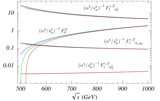
Figure 2: The singlet form factor $F_{0}^{Z}$ and the different contributions to the triplet form factor $F_{1}^{\gamma,Z}$ for $m_{H}=120$ GeV (respective upper lines), $m_{H}=140$ GeV (respective middles lines), and $m_{H}=160$ GeV (respective lower lines). Here, $F^{\gamma,Z}_{1,\lambda_{t}^{2}}$ refers to the contribution to $F_{1}^{\gamma,Z}$ which is proportional to $\lambda_{t}^{2}$, and $F^{\gamma,Z}_{1,\lambda_{t}\,g_{Z}}$ and $F^{\gamma,Z}_{1,g_{Z}^{2}}$ are defined analogously. The top mass is set to $m_{t}=180$ GeV and the other parameters are given in Eqs. (47).

We note that the NLL (${\cal O}(\alpha_{s})$) matching conditions for the three triplet Wilson coefficients $c_{1,j}$ depend on the $t\bar{t}$ spin configuration (i.e.  on $j$) since the kinematic situation for $t\bar{t}H$ production in the large Higgs energy end point is not invariant under separate rotations of the spin quantization axis. However, for our purposes it is sufficient to define a triplet Wilson coefficient that is averaged over the three spin configurations. Using such an averaged triplet Wilson coefficient the Higgs energy spectrum at NLL order can also be cast in the simple form of Eq. (37).

IV Matching Conditions at NLL Order

At NLL order, we need to account for the ${\cal O}(\alpha_{s}^{2})$ contributions to the Coulomb potential in Eq. (8), the NLL running of the coefficients $c_{1}$ and $c_{0}$ and their ${\cal O}(\alpha_{s})$ matching conditions at $\nu=1$. The latter QCD corrections are process specific and cannot be inferred from results obtained in earlier computations for the $t\bar{t}$ threshold in $e^{+}e^{-}\to t\bar{t}$.

Figure 3: Diagrams describing virtual one-loop QCD corrections in the Standard Model to compute the NLL matching conditions for the operators $J_{1,{\mbox{\scriptsize\boldmath$p$}}}$ and $J_{0,{\mbox{\scriptsize\boldmath$p$}}}$ that describe $t\bar{t}$ production for invariant masses $Q^{2}\approx 4m_{t}^{2}$. Self energy diagrams are implied.

Since we are interested in the region where $Q^{2}\approx 4m_{t}^{2}$ and we can neglect gluon exchange with the Higgs final state, we can apply the same nonrelativistic powercounting as the one known for the process $e^{+}e^{-}\to t\bar{t}$. Thus real gluon radiation, which is related to emission of gluons with energies of order $m_{t}v^{2}\sim m_{t}\alpha_{s}^{2}$ in the $t\bar{t}$ c.m. frame, is suppressed by a factor $\alpha_{s}\times(Q^{2}-4m_{t}^{2})/m^{2}\sim v^{3}$ (using the nonrelativistic counting $v\sim\alpha_{s}$). Therefore we only need to take into account the hard contributions contained in the virtual QCD corrections shown in Fig. 3. We have extracted the hard QCD corrections from the results for the Standard Model amplitude for $e^{+}e^{-}\to t\bar{t}H$ computed in Ref. Denner1 . The results of Ref. Denner1 were given in term of numerical codes for form factors to a number of standard matrix elements. We have computed the contributions of these form factors to $d\sigma/dE_{H}$ in the large Higgs energy region. To the result we have matched the corresponding expression for the ${\cal O}(\alpha_{s})$ corrections contained in the effective theory expression in Eq. (37) at $\mu=m_{t}$ ($\nu=1$). This allowed us to determine the ${\cal O}(\alpha_{s})$ matching conditions to $c_{0,1}$ numerically,

$$c_{0,1}(\nu=1)=1+\frac{C_{F}\alpha_{s}(m_{t})}{2}\,\delta c_{0,1}(\sqrt{s},m_{t},m_{H})\,.$$ (41)

$\delta c_{1}$		$\sqrt{s}$
$\quad m_{t}\quad$	$\quad m_{H}\quad$	$500$	$600$	$700$	$800$	$900$	$1000$
$175$	$120$	$-2.266(1)$	$-2.339(1)$	$-2.397(1)$	$-2.453(1)$	$-2.509(1)$	$-2.564(1)$
	$140$		$-2.339(1)$	$-2.401(1)$	$-2.459(1)$	$-2.516(1)$	$-2.572(1)$
	$160$		$-2.340(0)$	$-2.407(1)$	$-2.467(1)$	$-2.524(1)$	$-2.581(1)$
$180$	$120$	$-2.254(1)$	$-2.329(1)$	$-2.386(1)$	$-2.441(0)$	$-2.495(1)$	$-2.548(1)$
	$140$		$-2.327(1)$	$-2.389(1)$	$-2.446(1)$	$-2.501(1)$	$-2.555(1)$
	$160$		$-2.328(1)$	$-2.394(1)$	$-2.452(0)$	$-2.509(0)$	$-2.564(1)$

Table 1: Numerical values for the averaged spin triplet matching condition $\delta c_{1}(\sqrt{s},m_{t},m_{H})$ for typical values of $\sqrt{s}$, $m_{t}$ and $m_{H}$. The masses and energies are given in units of GeV.

$\delta c_{0}$		$\sqrt{s}$
$\quad m_{t}\quad$	$\quad m_{H}\quad$	$500$	$600$	$700$	$800$	$900$	$1000$
$175$	$120$	$-0.562(5)$	$-0.638(4)$	$-0.692(4)$	$-0.733(1)$	$-0.763(2)$	$-0.787(1)$
	$140$		$-0.636(3)$	$-0.691(4)$	$-0.732(3)$	$-0.762(2)$	$-0.786(1)$
	$160$		$-0.634(3)$	$-0.690(4)$	$-0.731(4)$	$-0.762(1)$	$-0.785(2)$
$180$	$120$	$-0.553(4)$	$-0.627(3)$	$-0.684(2)$	$-0.725(1)$	$-0.756(1)$	$-0.780(2)$
	$140$		$-0.625(4)$	$-0.682(4)$	$-0.725(4)$	$-0.755(2)$	$-0.780(2)$
	$160$		$-0.622(4)$	$-0.681(4)$	$-0.723(1)$	$-0.755(1)$	$-0.779(2)$

Table 2: Numerical values for the spin singlet matching condition $\delta c_{0}(\sqrt{s},m_{t},m_{H})$ for typical values of $\sqrt{s}$, $m_{t}$ and $m_{H}$. The masses and energies are given in units of GeV.

With this method the averaged triplet coefficient is obtained automatically. Since the numerical results of Ref. Denner1 are functions of the four-momenta of the initial and final state particles we were able to approach the large Higgs energy end point from several directions in the final state phase space in order to test the numerical stability and the independence of the result on the direction with which the end point is approached. For example, depending on the top-antitop quark c.m.  relative velocity $v$, the Higgs and the top and antitop quark four momenta (moving in the x-y plane to be definite) can be written as

$$p_{H} = (E_{H},0,k_{H},0)\,,$$

$$k_{1} = (E_{1},-|\mathbf{k}_{1}|\sin\theta,|\mathbf{k}_{1}|\cos\theta,0)\,,$$

$$k_{2} = (E_{2},-|\mathbf{k}_{2}|\sin(\bar{\theta}+\theta),|\mathbf{k}_{2}|\cos(\bar{\theta}+\theta),0)\,,$$ (42)

where

$$|\mathbf{k}_{i}| = \sqrt{E_{i}-m_{i}^{2}}\,,\qquad E_{H}\,=\,\frac{1}{2\sqrt{s}}\left(s+m_{H}^{2}-Q^{2}\right)\,,\qquad Q^{2}\,=\,\frac{4m_{t}^{2}}{1-v^{2}}\,,$$

$$E_{1} = \sqrt{s}-E_{H}-E_{2}\,,\qquad E_{2}\,=\,\frac{1}{2}\left(\sqrt{s}-E_{H}-\frac{\sqrt{s}}{2}\beta\right)\,,$$

$$\beta = \frac{x}{\sqrt{s}}\left(\frac{4(E_{H}^{2}-m_{H}^{2})\,(s-2\,\sqrt{s}\,E_{H}+m_{H}^{2}-4m_{t}^{2})}{(s-2\,\sqrt{s}\,E_{H}+m_{H}^{2})}\right)^{1/2}\,,$$

$$\bar{\theta} = \arccos\left[\,\frac{s+2m_{t}^{2}-2\,\sqrt{s}\,(E_{1}+E_{2})+2\,E_{1}\,E_{2}-m_{H}^{2}}{2|\mathbf{k}_{1}||\mathbf{k}_{2}|}\,\right]\,,$$

$$\theta = \arccos\left[\,\frac{E_{H}\,E_{1}-\sqrt{s}\,E_{1}+m_{t}^{2}+E_{1}\,E_{2}-|\mathbf{k}_{1}||\mathbf{k}_{2}|\,\cos\bar{\theta}}{|\mathbf{k}_{H}||\mathbf{k}_{1}|}\,\right]\,.$$ (43)

The variable $x$ can be chosen between $0$ and $1$ and interpolates between the two extreme situations $x=0$, which refers to the symmetric configuration where $E_{1}=E_{2}$, and $x=1$, which describes the situation where the top and antitop quarks move into the same direction having the maximal possible energy difference. We have extracted the functions $\delta c_{0,1}$ numerically in the limit $v\to 0$ and estimated the uncertainties from extrapolating to $v=0$ and from varying the variable $x$ between $0.1$ and $0.9$. For $x$ too close to zero or one the extraction procedure becomes unreliable due to numerical instabilities that develop in the code of Ref. Denner1 in these particular edges of the phase space. In order to identify the singlet and the triplet contributions in the full theory we used the helicity basis for the top and antitop spinors in the large Higgs energy end point where $k_{1}=k_{2}$ to construct the singlet and the three triplet $t\bar{t}$ spin configurations from the standard matrix elements given in Ref. Denner1 . The results (including our error estimate) for some representative values for $\sqrt{s}$, $m_{t}$ and $m_{H}$ are shown in Tab. 1 for $\delta c_{1}$ and in Tab. 2 for $\delta c_{0}$. In particular, for smaller c.m. energies we find that the absolute uncertainties for the singlet matching conditions are a few times larger than for the triplet matching conditions. This is a numerical effect that can be understood from the fact that for smaller c.m. energies the contributions coming from the singlet $t\bar{t}$ spin configuration are much smaller than those coming from the triplet spin configuration. In both cases, however, the relative uncertainties are well below 1%.

V Numerical Analysis

Figure 4: Higgs energy spectrum in the end point region at LL (dotted lines) and NLL (solid lines) order in the nonrelativistic expansion for the vNRQCD renormalization parameters $\nu=0.1,0.2,0.4$ and for $\sqrt{s}=600$ GeV, $m_{t}^{\rm 1S}=180$ GeV, $m_{H}=140$ GeV.

Figure 5: Higgs energy spectrum at LL (dotted lines) and NLL (solid lines) order in the nonrelativistic expansion for the vNRQCD renormalization parameters $\nu=0.1,0.2,0.4$ and at the Born level and at ${\cal O}(\alpha_{s})$ for $\mu=\sqrt{s},\sqrt{s}|v|$ for the parameters (a) $\sqrt{s}=500$ GeV, $m_{H}=120$ GeV, (b) $\sqrt{s}=550$ GeV, $m_{H}=140$ GeV, (c) $\sqrt{s}=600$ GeV, $m_{H}=140$ GeV, (d) $\sqrt{s}=700$ GeV, $m_{H}=140$ GeV. For all cases that top mass has been set to $m_{t}^{\rm 1S}=180$ GeV

$\sqrt{s}$ [GeV]	$m_{H}$ [GeV]	$\mbox{}\;\sigma(\mbox{Born})$ [fb]	$\mbox{}\;\sigma(\alpha_{s})$ [fb]	$\mbox{}\;\sigma(\mbox{NLL})$ [fb]	$\mbox{}\quad\frac{\sigma(\mbox{\tiny NLL})}{\sigma(\mbox{\tiny Born})}\quad\mbox{}$	$\mbox{}\quad\frac{\sigma(\mbox{\tiny NLL})}{\sigma(\alpha_{s})}\quad\mbox{}$	$\frac{\sigma(\mbox{\tiny NLL})_{|\beta|<0.2}}{\sigma(\alpha_{s})_{\beta<0.2}}$
$500$	$120$	$0.151$	$0.263$	$\quad 0.357(20)$	$2.362$	$1.359$	$1.78$
$550$	$120$	$0.984$	$1.251$	$\quad 1.342(37)$	$1.364$	$1.073$	$1.66$
$550$	$140$	$0.430$	$0.589$	$\quad 0.658(24)$	$1.530$	$1.117$	$1.68$
$550$	$160$	$0.134$	$0.207$	$\quad 0.254(12)$	$1.902$	$1.226$	$1.74$
$600$	$120$	$1.691$	$1.939$	$\quad 2.005(30)$	$1.185$	$1.034$	$1.66$
$600$	$140$	$1.014$	$1.203$	$\quad 1.259(24)$	$1.241$	$1.046$	$1.67$
$600$	$160$	$0.565$	$0.700$	$\quad 0.745(18)$	$1.319$	$1.065$	$1.68$
$700$	$120$	$2.348$	$2.454$	$\quad 2.485(13)$	$1.058$	$1.012$	$1.68$
$700$	$140$	$1.695$	$1.797$	$\quad 1.825(12)$	$1.077$	$1.016$	$1.69$
$700$	$160$	$1.210$	$1.303$	$\quad 1.328(11)$	$1.098$	$1.020$	$1.69$
$800$	$120$	$2.428$	$2.427$	$\quad 2.442(5)$	$1.006$	$1.006$	$1.73$
$800$	$140$	$1.880$	$1.893$	$\quad 1.908(5)$	$1.015$	$1.008$	$1.72$
$800$	$160$	$1.456$	$1.479$	$\quad 1.493(5)$	$1.025$	$1.009$	$1.72$
$900$	$120$	$2.290$	$2.229$	$\quad 2.237(6)$	$0.977$	$1.004$	$1.78$
$900$	$140$	$1.842$	$1.802$	$\quad 1.810(5)$	$0.982$	$1.005$	$1.78$
$900$	$160$	$1.489$	$1.463$	$\quad 1.471(3)$	$0.988$	$1.006$	$1.78$
$1000$	$120$	$2.087$	$1.997$	$\quad 2.002(8)$	$0.959$	$1.003$	$1.81$
$1000$	$140$	$1.721$	$1.651$	$\quad 1.656(7)$	$0.962$	$1.003$	$1.82$
$1000$	$160$	$1.429$	$1.375$	$\quad 1.380(5)$	$0.966$	$1.004$	$1.81$

Table 3: Collection of cross sections and K factors for various c.m. energies and Higgs masses and top quark mass $m_{t}^{\rm 1S}=180$ GeV.

In Fig. 4 the Higgs energy spectrum in the large energy end point region is displayed at LL (dashed lines) and NLL (solid lines) order in the nonrelativistic expansion for the vNRQCD renormalization parameters $\nu=0.1,0.2,0.4$ and for $\sqrt{s}=600$ GeV, $m_{t}^{\rm 1S}=180$ GeV, $m_{H}=140$ GeV, and

$$\begin{array}[]{ll}\Gamma_{t}=1.55~{}\mbox{GeV}\,,&\\ M_{Z}=91.1876~{}\mbox{GeV}\,,&\quad M_{W}=80.423~{}\mbox{GeV},\\ \alpha^{-1}=137.034\,,&\quad c_{w}=M_{W}/M_{Z}\,.\end{array}$$ (47)

At LL order the upper (lower) curve corresponds to $\nu=0.1$ ($0.4$), while at NLL order the upper (lower) curve corresponds to $\nu=0.2$ ($0.1$). The curves in Fig. 4 show the typical behavior of the nonrelativistic expansion for any choice of parameters. While the LL predictions have a quite large renormalization parameter dependence at the level of several tens of percent, the NLL results are stable. Here, the renormalization parameter variation is around 5%. The stabilization with respect to renormalization parameter variations at NLL order arises mainly from the inclusion of the ${\cal O}(\alpha_{s})$ QCD corrections to the Coulomb potential, Eq. (8). Moreover, the NLL curves lie considerably lower than the LL ones. This behavior is well known from the predictions for $e^{+}e^{-}\to t\bar{t}$ at threshold TTBARreview ; hmst and originates from the structure of the large negative ${\cal O}(\alpha_{s})$ QCD corrections to the Coulomb potential, Eq. (8), and from the sizable negative QCD corrections to the matching conditions in Eq. (41).

In principle this behavior is a point of concern because it could indicate that the renormalization parameter variation might be an inadequate method to estimate theoretical uncertainties. Fortunately, the top quark mass is sufficiently large such that the regions where the conventional fixed-order expansion (in powers of the strong coupling) and where the nonrelativistic expansion (described by the effective theory) can be applied are expected to overlap. In Figs. 5 the Higgs energy spectrum is displayed in the fixed-order expansion at the Born (dashed lines) and the ${\cal O}(\alpha_{s})$ level (solid lines) and in the nonrelativistic expansion at LL (dotted lines) and NLL order (solid lines). For the four panels we have chosen the parameters (a) $\sqrt{s}=500$ GeV, $m_{H}=120$ GeV, (b) $\sqrt{s}=550$ GeV, $m_{H}=140$ GeV, (c) $\sqrt{s}=600$ GeV, $m_{H}=140$ GeV, and (d) $\sqrt{s}=700$ GeV, $m_{H}=140$ GeV. For all cases we used $m_{t}^{\rm 1S}=180$ GeV as the top quark mass. The Born curves were obtained from the analytic results given in Ref. Dawson1 and the ${\cal O}(\alpha_{s})$ curves were obtained from the numerical program developed by Denner et al. in Ref. Denner1 . The two ${\cal O}(\alpha_{s})$ curves correspond to the renormalization scales $\mu=\sqrt{s}$ (lower curve) and $\mu=|\sqrt{s}v|$ (upper curve), where $v$ is the $t\bar{t}$ relative velocity defined in Eq. (16). The latter choice for the fixed-order renormalization scale is motivated by the fact that the relative momentum of the top pair is the scale that governs the Coulomb singularities contained in the fixed-order expansion close the large Higgs energy end point. This choice for the fixed-order renormalization scale is therefore the more appropriate one closer to the Higgs energy end point. For the nonrelativistic expansion the renormalization parameters $\nu=0.1,0.2,0.4$ were employed, as in Fig. 4. The results in Fig. 5a-d demonstrate that there is an overlap between the ${\cal O}(\alpha_{s})$ fixed-order prediction and the NLL nonrelativistic one in the region where the $t\bar{t}$ relative velocity is approximately 0.2. (The Higgs energy with $v=0.2$ is indicated in each panel by the solid vertical line.) The overlap improves for increasing c.m. energies or decreasing Higgs masses. This indicates that in the overlap regions the higher order contributions summed in the nonrelativistic prediction and the higher order relativistic corrections contained in the fixed-order result are both small. For smaller c.m. energies or increasing Higgs masses, on the other hand, the NLL nonrelativistic predictions tend to lie slightly above the ${\cal O}(\alpha_{s})$ fixed-order results (for $\mu=\sqrt{s}v$) illustrating the impact of the higher order corrections to each type of expansion. The discrepancy, however, remains comparable to the uncertainties estimated from the renormalization parameter variation of the NLL nonrelativistic prediction. We therefore conclude that the renormalization parameter variation of the NLL order nonrelativistic prediction should provide a realistic estimate of the theoretical uncertainties in the large Higgs energy region.

Finally, let us discuss the numerical impact of the nonrelativistic contributions in the large Higgs energy region on the total cross section. The results in Figs. 5 show that the summation of the Coulomb singularities and the logarithms of the top quark velocity lead to an enhancement of the cross section and that the portion of phase space where nonrelativistic effects are important increases for decreasing c.m. energy or increasing Higgs mass. In Tab. 3 the impact of the summations is analyzed numerically for various choices of the c.m. energy and the Higgs mass. For all cases the top quark mass $m_{t}^{\rm 1S}=180$ GeV was used. The other parameters are fixed as in Figs. 4 and 5 discussed earlier. In the table $\sigma(\mbox{Born})$ refers to the Born cross section and $\sigma(\alpha_{s})$ to the ${\cal O}(\alpha_{s})$ cross section in fixed-order perturbation theory using $\mu=\sqrt{s}$ as the renormalization scale, the choice employed in the analysis of Ref. Denner1 . All cross sections are given in fb units. The term $\sigma(\mbox{NLL})$ refers to the sum of the ${\cal O}(\alpha_{s})$ fixed-order cross section for $v>0.2$ using $\mu=\sqrt{s}v$ and the NLL nonrelativistic cross section for $|v|<0.2$ with the renormalization parameter $\nu=0.2$. The numbers for $\sigma(\mbox{NLL})$ represent the currently most complete predictions for the total cross section of the process $e^{+}e^{-}\to t\bar{t}H$ as far as QCD corrections are concerned. For the results for $\sigma(\mbox{NLL})$ we have also given our estimate for the theoretical error. For the fixed-order contribution ($v>0.2$) we have estimated the uncertainty by taking the maximum of the shifts obtained from varying $\mu$ in the ranges $[\sqrt{s},2\sqrt{s}]$, $[\sqrt{s},\sqrt{s}/2]$ and $[\sqrt{s}v,\sqrt{s}]$; for the nonrelativistic contribution in the end point we have assumed an uncertainty of 5% for all cases. For the errors given in Tab. 3 both uncertainties were added linearly.

The results show that the effect of the summations in the large Higgs energy region is particularly important for smaller c.m. energies and larger Higgs masses, when the portion of the phase space where the nonrelativistic expansion has to be applied is large. Here, the higher order summations contained in the nonrelativistic expansion can be comparable to the already sizable ${\cal O}(\alpha_{s})$ fixed-order corrections and enhance the cross section further. This is advantageous for top Yukawa coupling measurements for the lower c.m. energies that are accessible in the first phase of the International Linear Collider experiment. For higher c.m. energies the effect of the nonrelativistic summations of contributions from beyond ${\cal O}(\alpha_{s})$ is less pronounced and decreases to the one-percent level for c.m. energies above $700$ GeV, see column seven of Tab. 3. For all cases, except for very large c.m. energies around $1000$ GeV, however, the shift caused by the terms that are summed up in the nonrelativistic expansion exceeds the theoretical error. In the last column we have also displayed the ratio of the NLL nonrelativistic cross section for $|v|<0.2$ with $\nu=0.2$ and the ${\cal O}(\alpha_{s})$ fixed-order cross section for $v<0.2$ with $\mu=\sqrt{s}$ to illustrate the effect of the summation of QCD corrections beyond one loop that have to be carried out in the large Higgs energy region. Interestingly, the higher order summations lead to correction factors ranging between about $1.7$ and $1.8$ that are only very weakly dependent of the c.m. energy and the Higgs mass. This fact might prove useful for rough implementations of nonrelativistic $t\bar{t}$ effects in other high energy processes.

VI Conclusion

In this paper we have computed the Higgs energy distribution for the process $e^{+}e^{-}\to t\bar{t}H$ in the large Higgs energy end point region. Due to Coulomb singularities $\sim(\alpha_{s}/v)^{n}$ and logarithmic divergences $\sim(\alpha_{s}\ln v)^{n}$ that arise at higher order of conventional multiloop-perturbation theory in the large Higgs energy end point region, $v$ being the top velocity in the $t\bar{t}$ c.m. frame, usual fixed-order perturbation theory breaks down. We use the nonrelativistic effective theory vNRQCD to sum both types of singular terms and determine the Higgs energy distribution in the end point region at next-to-leading logarithmic order. While the Coulomb singularities are summed by solving the nonrelativistic equation of motion for the $t\bar{t}$ Green function, the logarithmic terms are summed using the renormalization group equations in the effective theory. We have compared the effective theory predictions for the Higgs energy spectrum with the ${\cal O}(\alpha_{s})$ fixed-order results from Ref. Denner1 and can show that the nonrelativistic and the fixed-order expansion (with the renormalization scale $\mu$ set of order $\sqrt{s}\,v$) have a region of overlap where $v$ is around $0.2$. For our next-to-leading logarithmic order effective theory prediction we estimate a theoretical error of 5%. The summations lead to an additional sizable enhancement of the total cross section compared to the positive ${\cal O}(\alpha_{s})$ fixed-order corrections and are particularly important for lower c.m. energies (or larger Higgs masses) where the portion of the phase space where the $t\bar{t}$ QCD dynamics is nonrelativistic is increased. For higher energies the effects decrease and reach the one percent level at c.m. energies around $700$ GeV. We have given updated predictions for the total cross section $\sigma(e^{+}e^{-}\to t\bar{t}H)$ combining our effective theory next-to-leading logarithmic prediction in the large Higgs energy region with the fixed-order ${\cal O}(\alpha_{s})$ results determined in Ref. Denner1 .

References

• (1) R. Barate et al. [ALEPH Collaboration], Phys. Lett. B 565, 61 (2003) [arXiv:hep-ex/0306033].
• (2) P. B. Renton, arXiv:hep-ph/0410177.
• (3) J. A. Aguilar-Saavedra et al. [ECFA/DESY LC Physics Working Group Collaboration], arXiv:hep-ph/0106315.
• (4) T. Abe et al. [American Linear Collider Working Group Collaboration], in Proc. of the APS/DPF/DPB Summer Study on the Future of Particle Physics (Snowmass 2001) ed. N. Graf, arXiv:hep-ex/0106057; T. Abe et al. [American Linear Collider Working Group], Linear Collider Physics Resource Book for Snowmass 2001 (SLAC, Stanford, CA, 2001) arXiv:hep-ex/0106056.
• (5) K. Abe et al. [ACFA Linear Collider Working Group Collaboration], arXiv:hep-ph/0109166.
• (6) K. J. F. Gaemers and G. J. Gounaris, Phys. Lett. B 77, 379 (1978); A. Djouadi, J. Kalinowski and P. M. Zerwas, Mod. Phys. Lett. A 7, 1765 (1992); A. Djouadi, J. Kalinowski and P. M. Zerwas, Z. Phys. C 54, 255 (1992).
• (7) S. Dawson and L. Reina, Phys. Rev. D 57, 5851 (1998) [arXiv:hep-ph/9712400].
• (8) S. Dawson and L. Reina, Phys. Rev. D 59, 054012 (1999) [arXiv:hep-ph/9808443].
• (9) S. Dittmaier, M. Kramer, Y. Liao, M. Spira and P. M. Zerwas, Phys. Lett. B 441, 383 (1998) [arXiv:hep-ph/9808433].
• (10) G. Belanger et al., Phys. Lett. B 571, 163 (2003) [arXiv:hep-ph/0307029].
• (11) A. Denner, S. Dittmaier, M. Roth and M. M. Weber, Nucl. Phys. B 680, 85 (2004) [arXiv:hep-ph/0309274].
• (12) Y. You, W. G. Ma, H. Chen, R. Y. Zhang, S. Yan-Bin and H. S. Hou, Phys. Lett. B 571, 85 (2003) [arXiv:hep-ph/0306036].
• (13) A. Djouadi, J. Kalinowski and M. Spira, Comput. Phys. Commun.  108, 56 (1998) [arXiv:hep-ph/9704448].
• (14) A. H. Hoang, arXiv:hep-ph/0204299; A. H. Hoang et al., Eur. Phys. J. directC 2, 1 (2000) [arXiv:hep-ph/0001286].
• (15) M.E. Luke, A.V. Manohar and I.Z. Rothstein, Phys. Rev.  D61, 074025 (2000) [arXiv:hep-ph/9910209].
• (16) A.V. Manohar and I.W. Stewart, Phys. Rev. D 62, 014033 (2000) [arXiv:hep-ph/9912226].
• (17) A.V. Manohar and I.W. Stewart, Phys. Rev.  D62, 074015 (2000) [arXiv:hep-ph/0003032].
• (18) A. H. Hoang and I. W. Stewart, Phys. Rev. D 67, 114020 (2003) [arXiv:hep-ph/0209340].
• (19) A. H. Hoang, A. V. Manohar, I. W. Stewart and T. Teubner, Phys. Rev. Lett.  86, 1951 (2001) [arXiv:hep-ph/0011254]; and Phys. Rev. D 65, 014014 (2002) [arXiv:hep-ph/0107144].
• (20) N. Brambilla, A. Pineda, J. Soto and A. Vairo, arXiv:hep-ph/0410047.
• (21) A. H. Hoang and C. J. Reisser, Phys. Rev. D71, 074022 (2005), arXiv:hep-ph/0412258.
• (22) U. Aglietti and Z. Ligeti, Phys. Lett. B 364, 75 (1995) [arXiv:hep-ph/9503209].
• (23) A. H. Hoang, M. C. Smith, T. Stelzer and S. Willenbrock, Phys. Rev. D 59, 114014 (1999) [arXiv:hep-ph/9804227]; M. Beneke, Phys. Lett. B 434, 115 (1998) [arXiv:hep-ph/9804241]; A. Pineda, PhD Thesis, Univ. Barcelona (1998).
• (24) A. H. Hoang, Z. Ligeti and A. V. Manohar, Phys. Rev. Lett.  82, 277 (1999) [arXiv:hep-ph/9809423]; A. H. Hoang, Z. Ligeti and A. V. Manohar, Phys. Rev. D 59, 074017 (1999) [arXiv:hep-ph/9811239].
• (25) A. H. Hoang and T. Teubner, Phys. Rev. D 60, 114027 (1999) [arXiv:hep-ph/9904468].
• (26) A. H.  Hoang, Phys. Rev. D 69, 034009 (2004) [arXiv:hep-ph/0307376].
• (27) W. Fischler, Nucl. Phys. B 129, 157 (1977).
• (28) A. Billoire, Phys. Lett. B92, 343 (1980).
• (29) A. Pineda, Phys. Rev. D 66, 054022 (2002) [arXiv:hep-ph/0110216].
• (30) A. A. Penin and A. A. Pivovarov, Phys. Lett. B 435, 413 (1998) [arXiv:hep-ph/9803363].
• (31) M. Jeżabek, J. H. Kühn and T. Teubner, Z. Phys.  C56, 653 (1992).
• (32) M. J. Strassler and M. E. Peskin, Phys. Rev.  D43, 1500 (1991).
• (33) S. Dawson, private communication.