Mesons and diquarks in the color neutral 2SC phase of dense cold quark matter

Abstract

The spectrum of meson and diquark excitations of dense color neutral cold quark matter is investigated in the framework of a 2-flavored Nambu–Jona-Lasinio type model, including a quark $\mu$- and color $\mu_{8}$ chemical potential. It was found out that in the color superconducting (2SC) phase, i.e. at $\mu>\mu_{c}=342$ MeV, $\mu_{8}$ aquires rather small values $\sim$ 10 MeV in order to ensure the color neutrality. In this phase the $\pi$- and $\sigma$ meson masses are evaluated around $\sim$ 330 MeV. The spectrum of scalar diquarks in the color neutral 2SC phase consists of a heavy ($\rm SU_{c}(2)$-singlet) resonance with mass $\sim$ 1100 MeV, four light diquarks with mass $3|\mu_{8}|$, and one Nambu –Goldstone boson which is in accordance with the Goldstone theorem. Moreover, in the 2SC phase there are five light stable particles as well as a heavy resonance in the spectrum of pseudo-scalar diquarks. In the color symmetric phase, i.e. for $\mu<\mu_{c}$, a mass splitting of scalar diquarks and antidiquarks is shown to arise if $\mu\neq 0$, contrary to the case of $\mu=0$, where the masses of scalar antidiquarks and diquarks are degenerate at the value $\sim$ 700 MeV. If the coupling strength in the pseudo-scalar diquark channel is the same as in the scalar diquark one (as for QCD-inspired NJL models), then in the color symmetric phase pseudo-scalar diquarks are not allowed to exist as stable particles.

I Introduction

Recent investigations, performed in the framework of perturbative QCD, show that at low temperatures and asymptotically high values of the quark chemical potential $\mu$ the dense baryonic matter is a color superconductor son . Evidently, at rather small values of $\mu$ a more adequate description of this phenomenon can be done with the help of different effective models, such as Nambu – Jona-Lasinio- (NJL) type field theories with four-fermionic interaction njl , etc. In such a way, on the basis of NJL-type models with two quark flavors it was shown that the color superconducting (2SC) phase might be yet present at rather small values of $\mu\sim 350$ MeV, i.e. at baryon densities only several times larger, than the density of ordinary nuclear matter (see reviews alford ; hs ). (For simplicity, throughout the paper we will study quark matter, composed from two quark flavors, i.e. up- and down quarks, only.) This is just the density of compact star cores. So, color superconductivity, which is eventually existing inside compact stars, might influence different observable astrophysical processes, and thus deserves to be studied in more details.

In the early NJL approach to color superconductivity skp ; bvy03 , the density of the color charge $Q_{8}$ was not constraint to zero in the 2SC ground state (the densities of other color charges $Q_{i}$, where $i=1,..,7$, are zero in this phase bh ) leading to a nonvanishing difference between the densities of red/green quarks and blue ones. In this case, the mesonic and diquark excitations of dense quark matter were considered in the framework of a simple two-flavored NJL model with a single quark chemical potential $\mu$ bekvy ; eky . In particular, it was shown that in the color asymmetric 2SC phase of this model does arise an abnormal number of three Nambu – Goldstone bosons (NG) instead of expected five , and $\pi$-mesons are stable excitations of its ground state with masses $\sim 300$ MeV. Besides, there are two light stable scalar diquark modes, whose masses are proportional to $\langle Q_{8}\rangle$, as well as one heavy scalar diquark resonance in the 2SC phase.

In reality, however, i.e. possibly in compact star cores or in relativistic heavy ion experiments, there are several physical constraints on the quark matter. The most evident one is its color neutrality, which means a vanishing of a bulk $Q_{i}$ color charges ($i=1,...,8$). Indeed, since the lump of quark matter, which might be created after heavy ion collisions, originated from color neutral objects and is surrounded by a color neutral medium, it is expected to be globally color neutral. To fulfill this requirement, usually the local color neutrality constraint is imposed by introducing several new chemical potentials, $\mu_{3}$, $\mu_{8}$, etc, into a NJL model hs ; mhuang ; zhuang . Otherwise, there will be produced a chromo-electric field resulting in the flow of color charges, so a homogeneous and color conducting quark medium with nonzero color charge densities is not allowed to be a stable one mhuang . (Recall, there is no need to add new chemical potentials into QCD. The point is that in the QCD 2SC ground state a nonzero value of the eightth gluon field component might be generated. Effectively, it is the $\mu_{8}$-chemical potential, so color neutrality is fulfilled automatically in the QCD approach rebhan .)

In the present paper, in contrast to our previous investigations bekvy ; eky , we study the mesonic and diquark excitations of color neutral quark matter in the framework of a simple two flavor NJL model at zero temperature. We consider both the case of rather small values of the quark chemical potential $\mu$ (the $SU_{c}(3)$ color symmetric (normal) phase), and the case of $\mu$-values, corresponding to the 2SC phase of the model. In addition, the properties of pseudo-scalar diquarks are also included into the consideration.

The paper is organized as follows. In Section II the thermodynamic potential as well as the effective action of the NJL model, extended by an additional color $\mu_{8}$-chemical potential term, is obtained in the one quark loop approximation. Further, in Section III, the gap equations and the phase structure of the model is investigated under the color neutrality constraint. Here the values of $\mu_{8}$ are obtained at which the 2SC phase is a color neutral one. Then, in the Sections IV, V, and VI, the masses of the $\pi$- and $\sigma$ mesons, scalar diquarks, and pseudo-scalar diquarks are considered, respectively. Finally, in the Appendix, the influence of the mixing between $\sigma$-meson and scalar diquarks on the $\sigma$-mass is discussed.

II The model and its effective action

In the original version of the NJL model njl the four-fermionic interaction of a proton $p$ and neutron $n$ doublet was considered, and the principle of dynamical chiral symmetry breaking was demonstrated. Later, the $(p,n)$-doublet was replaced by a doublet of colored up $u$ and down $d$ quarks, in order to describe phenomenologically the physics of light mesons ebvol ; volk ; hatsuda ; volkyud , diquarks ebka ; vog , as well as meson-baryon interactions ebjur ; reinh . In this sense the NJL model may be thought of as an effective theory for low energy QCD. (Of course, it is necessary to remember that in the NJL model, in contrast with QCD, quarks are not confined in the hardronic phase, which is a shortcoming of the model.) At present time the phenomenon of dynamical (chiral) symmetry breaking is one of the cornerstones of modern physics. So, this effect was studied in the framework of NJL-type models under the influence of external magnetic fields mir , in curved space-times odin , in spaces with nontrivial topology incera , etc. Formally, as it was mentioned above, quarks are presented in the mass spectrum of the model. So it is very suitable for the description of normal hot and/or dense quark matter hatsuda ; asakawa ; ebert ; klim in which, as it is known, quarks are not confined. NJL-type models still remain a simple but useful instrument for studying color superconducting quark matter at moderate densities alford ; hs ; skp ; bvy03 , where analytical and lattice computations in the framework of QCD are impossible.

We start from the following 2-flavor NJL Lagrangian, called for the description of interactions in the quark-antiquark, scalar diquark- as well as pseudo-scalar diquark channels at low and moderate energies and baryon densities (the consideration is performed in Minkovski space-time notation):

$$L_{q}=\bar{q}\Big{[}\gamma^{\nu}i\partial_{\nu}-m_{0}+\mu\gamma^{0}\Big{]}q+G\Big{\{}(\bar{q}q)^{2}+(\bar{q}i\gamma^{5}\vec{\tau}q)^{2}\Big{\}}+$$ (1)

$$+ \!\!\!\sum_{A=2,5,7}\Big{\{}H_{s}[\bar{q}^{C}i\gamma^{5}\tau_{2}\lambda_{A}q][\bar{q}i\gamma^{5}\tau_{2}\lambda_{A}q^{C}]+H_{p}[\bar{q}^{C}\tau_{2}\lambda_{A}q][\bar{q}\tau_{2}\lambda_{A}q^{C}]\Big{\}},$$

where $\mu>0$ is the quark chemical potential, the quark field $q\equiv q_{i\alpha}$ is a flavor doublet and color triplet as well as a four-component Dirac spinor, where $i=1,2$ (or $i=u,d$) and $\alpha=1,2,3$ (or $\alpha=r,g,b$). $q^{C}=C\bar{q}^{t}$, $\bar{q}^{C}=q^{t}C$ are charge-conjugated spinors, and $C=i\gamma^{2}\gamma^{0}$ is the charge conjugation matrix (symbol $t$ denotes the transposition operation). It is supposed that up and down quarks have equal current (bare) mass $m_{0}$. Furthermore, we use the notations $\tau_{a}$ for Pauli matrices, and $\lambda_{A}$ for antisymmetric Gell-Mann matrices in flavor and color space, respectively. Clearly, the Lagrangian $L_{q}$ is invariant under transformations from the color $\rm SU_{c}(3)$- as well as baryon $\rm U_{B}(1)$ groups. In addition, at $m_{0}=0$ this Lagrangian is symmetric under the chiral $\rm SU(2)_{L}\times SU(2)_{R}$ group (chiral transformations act on the flavor indices of quark fields only). Moreover, since $Q=I_{3}+B/2$, where $I_{3}=\tau_{3}/2$ is the generator of the third isospin component, $Q$ is the generator of the electric charge, and $B$ is the baryon charge generator, our system is symmetric under the electromagnetic group $\rm U_{Q}(1)$ as well. If the Lagrangian (1) is obtained from the QCD one-gluon exchange approximation, then $G:H_{s}:H_{p}=4:3:3$. However, in the present consideration we will not fix relations between coupling constants, so they are treated as free parameters. It is necessary to note also that at $\mu=0$ the Lagrangian (1) is invariant under the charge conjugation symmetry ($q\to q^{C}\equiv C\bar{q}^{t}$, $\bar{q}\to\bar{q}^{C}\equiv q^{t}C$) that is, however, spoiled by the chemical potential term.

Furtheron, the temperature is chosen to be zero throughout the paper. In this case there is a critical value $\tilde{\mu}_{c}$ of the chemical potential, such that at $\mu<\tilde{\mu}_{c}$ the color symmetric (normal) phase is realized in the system (evidently, the ground state of this phase is a color singlet). However, at $\mu>\tilde{\mu}_{c}$ one obtains a color superconducting (2SC) phase in which $\rm SU_{c}(3)$ is spontaneously broken down to $\rm SU_{c}(2)$. Only two quark colors, say red and green, participate in the gap formation in the 2SC phase, the blue quarks stay gapless. So the densities of red/green quarks, $n_{r,g}$, are equal in this phase, however the density $n_{b}$ of blue quarks is not equal to $n_{r,g}$, i.e. local color neutrality is broken. To restore local color neutrality in the 2SC phase of the model (1), usually an additional chemical potential term $\mu_{8}Q_{8}$ is introduced into the considerations hs , where $Q_{8}=\bar{q}\gamma^{0}T_{8}q$, and $T_{8}=$diag$(1,1,-2)=\sqrt{3}\lambda_{8}$ is the matrix in the color space. Hence,

$$L_{q}\to L=L_{q}+\mu_{8}Q_{8}.$$ (2)

If $\mu_{8}$ is an independent model parameter, then Lagrangian (2) is symmetric under the color $\rm SU_{c}(2)\times U_{\lambda_{8}}(1)$ group. However, if local color neutrality is imposed, then the chemical potential $\mu_{8}$ is not an independent parameter. Its value must be chosen in such a way that the ground state expectation value $\langle Q_{8}\rangle$ is identically equal to zero. Hence, $\mu_{8}$ depends on $\mu$ etc. For example, in the color symmetric phase, i.e. at $\mu<\mu_{c}$ (it will be shown in section III that in general case $\mu_{c}\neq$ $\tilde{\mu}_{c}$), where $\langle Q_{8}\rangle\equiv 0$ even in the theory (1), we have to put $\mu_{8}\equiv 0$. However $\mu_{8}$ has a nontrivial $\mu$-dependence at $\mu>\mu_{c}$ in order to supply the zero value of $\langle Q_{8}\rangle$. As a consequence, we see that the color symmetry group of the model (2) depends on $\mu$: at $\mu<\mu_{c}$ it is $\rm SU_{c}(3)$, whereas at $\mu>\mu_{c}$ it is the $\rm SU_{c}(2)\times U_{\lambda_{8}}(1)$ subgroup of $\rm SU_{c}(3)$ which is just the color symmetry group of the term $\mu_{8}Q_{8}$.

In the present paper we are going to study both the ground state properties of the system with Lagrangian $L$, and its mass spectrum in the quark-, meson- and diquark sectors. So, we have to obtain the thermodynamic potential $\Omega$ as well as the effective action of the model up to a second order in the bosonic degrees of freedom. To begin with, let us introduce the linearized version of Lagrangian $L$ that contains auxiliary bosonic fields:

$$\tilde{L}\displaystyle = \bar{q}\Big{[}\gamma^{\nu}i\partial_{\nu}+\mu\gamma^{0}+\mu_{8}T_{8}-\sigma-m_{0}-i\gamma^{5}\pi_{a}\tau_{a}\Big{]}q-\frac{1}{4G}\Big{[}\sigma\sigma+\pi_{a}\pi_{a}\Big{]}-\frac{1}{4H_{s}}\Delta^{s*}_{A}\Delta^{s}_{A}-\frac{1}{4H_{p}}\Delta^{p*}_{A^{\prime}}\Delta^{p}_{A^{\prime}}-$$ (3)

$$- \frac{\Delta^{s*}_{A}}{2}[\bar{q}^{C}i\gamma^{5}\tau_{2}\lambda_{A}q]-\frac{\Delta^{s}_{A}}{2}[\bar{q}i\gamma^{5}\tau_{2}\lambda_{A}q^{C}]-\frac{\Delta^{p*}_{A^{\prime}}}{2}[\bar{q}^{C}\tau_{2}\lambda_{A^{\prime}}q]-\frac{\Delta^{p}_{A^{\prime}}}{2}[\bar{q}\tau_{2}\lambda_{A^{\prime}}q^{C}],$$

where as well as in the following the summation over repeated indices $a=1,2,3$ and $A,A^{\prime}=2,5,7$ is implied. Lagrangians $L$ and $\tilde{L}$ are equivalent on the equations of motion for bosonic fields, from which it follows that

$$\sigma(x)=-2G(\bar{q}q),~{}~{}~{}\Delta^{s}_{A}(x)\!\! = \!\!-2H_{s}(\bar{q}^{C}i\gamma^{5}\tau_{2}\lambda_{A}q),~{}~{}~{}\Delta^{s*}_{A}(x)=-2H_{s}(\bar{q}i\gamma^{5}\tau_{2}\lambda_{A}q^{C}),$$

$$\pi_{a}(x)=-2G(\bar{q}i\gamma^{5}\tau_{a}q),~{}~{}~{}\Delta^{p}_{A^{\prime}}(x)\!\! = \!\!-2H_{p}(\bar{q}^{C}\tau_{2}\lambda_{A^{\prime}}q),~{}~{}~{}\Delta^{p*}_{A^{\prime}}(x)=-2H_{p}(\bar{q}\tau_{2}\lambda_{A^{\prime}}q^{C}).$$ (4)

One can easily see from (4) that mesonic fields $\sigma,\pi_{a}$ are real quantities, i.e. $(\sigma(x))^{\dagger}=\sigma(x),~{}~{}(\pi_{a}(x))^{\dagger}=\pi_{a}(x)$ (the superscript symbol $\dagger$ denotes the hermitian conjugation), but all diquark fields $\Delta^{s,p}_{A}$ are complex ones, so

$$(\Delta^{s}_{A}(x))^{\dagger}=\Delta^{s*}_{A}(x),~{}~{}~{}~{}~{}(\Delta^{p}_{A^{\prime}}(x))^{\dagger}=\Delta^{p*}_{A^{\prime}}(x).$$

Moreover, $\Delta^{s}_{A}$ and $\Delta^{p}_{A^{\prime}}$ are scalars and pseudo-scalars, correspondingly. Clearly, the real $\sigma$ and $\pi_{a}$ fields are color singlets, all scalar diquarks $\Delta^{s}_{A}$ form a color antitriplet $\bar{3}_{c}$ of the $\rm SU_{c}(3)$ group. The same is true for pseudo-scalar diquarks $\Delta^{p}_{A^{\prime}}$ which are also the components of an $\bar{3}_{c}$-multiplet of the color group. Evidently, in the $\rm SU_{c}(3)$-color symmetric phase (at $\mu<\mu_{c}$) all diquark fields must have zero ground state expectation values, i. e. $\langle\Delta^{s}_{A}\rangle=0$ and $\langle\Delta^{p}_{A^{\prime}}\rangle=0$. Otherwise, we have an indication that the ground state of the system is no more an $\rm SU_{c}(3)$-invariant one.

Lagrangian (3) provides us with a common footing for obtaining both the thermodynamic potential (TDP) and the mass spectrum for bosonic excitations. Indeed, in the one-fermion loop approximation, the effective action for the boson fields is expressed through the path integral over quark fields:

$$\exp(i{\cal S}_{\rm{eff}}(\sigma,\pi_{a},\Delta^{s,p}_{A},\Delta^{s,p*}_{A^{\prime}}))=N^{\prime}\int[d\bar{q}][dq]\exp\Bigl{(}i\int\tilde{L}\,d^{4}x\Bigr{)},$$

where

$${\cal S}_{\rm{eff}}(\sigma,\pi_{a},\Delta^{s,p}_{A},\Delta^{s,p*}_{A^{\prime}})=-\int d^{4}x\left[\frac{\sigma^{2}+\pi^{2}_{a}}{4G}+\frac{\Delta^{s}_{A}\Delta^{s*}_{A}}{4H_{s}}+\frac{\Delta^{p}_{A^{\prime}}\Delta^{p*}_{A^{\prime}}}{4H_{p}}\right]+\tilde{\cal S}_{\rm{eff}},$$ (5)

$N^{\prime}$ is a normalization constant. The quark contribution term $\tilde{\cal S}_{\rm{eff}}$ is here given by:

$$\exp(i\tilde{\cal S}_{\rm{eff}})=N^{\prime}\int[d\bar{q}][dq]\exp\Bigl{(}\frac{i}{2}\int\Big{[}\bar{q}D^{+}q+\bar{q}^{C}D^{-}q^{C}-\bar{q}Kq^{C}-\bar{q}^{C}K^{*}q\Big{]}d^{4}x\Bigr{)}.$$ (6)

In (6) we have used the following notations

$$D^{+}=i\gamma^{\nu}\partial_{\nu}-m_{0}+\hat{\mu}\gamma^{0}-\Sigma,~{}~{}~{}~{}~{}~{}~{}D^{-}=i\gamma^{\nu}\partial_{\nu}-m_{0}-\hat{\mu}\gamma^{0}-\Sigma^{t},~{}~{}~{}~{}~{}~{}~{}\Sigma=\sigma+i\gamma^{5}\pi_{a}\tau_{a},$$

$$\Sigma^{t}=\sigma+i\gamma^{5}\pi_{a}\tau^{t}_{a},~{}~{}~{}~{}~{}K^{*}=(\Delta^{p*}_{A}+i\Delta^{s*}_{A}\gamma^{5})\tau_{2}\lambda_{A},\qquad K=(\Delta^{p}_{A}+i\Delta^{s}_{A}\gamma^{5})\tau_{2}\lambda_{A},$$ (7)

where $D^{\pm}$ are nontrivial operators in the coordinate, spinor, color and flavor spaces. In the framework of the Nambu-Gorkov formalism, where quarks are composed into a bispinor $\Psi=\left({q\atop q^{C}}\right)$, it is possible to integrate in (6) over quark fields and obtain

$$\tilde{\cal S}_{\rm{eff}}(\sigma,\pi_{a},\Delta^{s,p}_{A},\Delta^{s,p*}_{A^{\prime}})=\frac{1}{2i}{\rm Tr}_{\{NGsfcx\}}\ln\left(\begin{array}[]{cc}D^{+}~{},&-K\\ -K^{*},&D^{-}\end{array}\right)\equiv\frac{1}{2i}{\rm Tr}_{\{NGsfcx\}}\ln Z.$$ (8)

Besides of an evident trace in the two-dimensional Nambu-Gorkov space (NG), the Tr-operation in (8) stands for calculating the trace in spinor- ($s$), flavor- ($f$), color- ($c$) as well as four-dimensional coordinate- ($x$) spaces, correspondingly.

Starting from (5)-(8), it is possible to define the thermodynamic potential $\Omega(\sigma,\pi_{a},\Delta^{s,p}_{A},\Delta^{s,p*}_{A^{\prime}})$ of the model:

$${\cal S}_{\rm{eff}}~{}\bigg{|}_{~{}\sigma,\pi_{a},\Delta^{s,p}_{A},\Delta^{s,p*}_{A^{\prime}}=\rm{const}}=-\Omega(\sigma,\pi_{a},\Delta^{s,p}_{A},\Delta^{s,p*}_{A^{\prime}})\int d^{4}x,$$ (9)

where, in the spirit of the mean-field approximation, all boson fields are supposed to be $x$-independent. It is well-known that ground state expectation values $\langle\sigma(x)\rangle\equiv\sigma^{o},~{}\langle\pi_{a}(x)\rangle\equiv\pi_{a}^{o},~{}\langle\Delta^{s,p}_{A}(x)\rangle\equiv\Delta^{s,po}_{A},~{}\langle\Delta^{s,p*}_{A^{\prime}}(x)\rangle\equiv\Delta^{s,p*o}_{A^{\prime}}$ are coordinates of the global minimum point of the thermodynamic potential $\Omega$, i.e. they form a solution of the gap equations (evidently, in our approach all ground state expectation values do not depend on coordinates $x$):

$$\frac{\partial\Omega}{\partial\pi_{a}}=0,~{}~{}~{}~{}~{}\frac{\partial\Omega}{\partial\sigma}=0,~{}~{}~{}~{}~{}\frac{\partial\Omega}{\partial\Delta^{s,p}_{A}}=0,~{}~{}~{}~{}~{}\frac{\partial\Omega}{\partial\Delta^{s,p*}_{A^{\prime}}}=0.$$ (10)

Let us make the following shift of bosonic fields in ${\cal S}_{\rm{eff}}$: $\sigma(x)\to\sigma(x)+\sigma^{o}$, $\pi_{a}(x)\to\pi_{a}(x)+\pi_{a}^{o}$, $\Delta^{s,p*}_{A}(x)\to\Delta^{s,p*}_{A}(x)+\Delta^{s,p*o}_{A}$, $\Delta^{s,p}_{A}(x)\to\Delta^{s,p}_{A}(x)+\Delta^{s,po}_{A}$, where $\sigma^{o},\pi^{o}_{a},\Delta^{s,po}_{A},\Delta^{s,p*o}_{A}$ have no coordinate dependency. In this case the matrix $Z$ from (8) is transformed in the following way:

$$Z\rightarrow\left(\begin{array}[]{cc}D^{+}_{o}~{},&-K_{o}\\ -K_{o}^{*}~{},&D^{-}_{o}\end{array}\right)-\left(\begin{array}[]{cc}\Sigma~{},&K\\ K^{*}~{},&\Sigma^{t}\end{array}\right)\equiv S_{0}^{-1}-\left(\begin{array}[]{cc}\Sigma~{},&K\\ K^{*}~{},&\Sigma^{t}\end{array}\right),$$ (11)

where $S_{0}$ is the quark propagator matrix in the Nambu-Gorkov representation, and

$$(K_{o},K^{*}_{o},D^{\pm}_{o},\Sigma_{o},\Sigma^{t}_{o})=(K,K^{*},D^{\pm},\Sigma,\Sigma^{t})~{}\bigg{|}_{~{}\sigma=\sigma^{o},\pi_{a}=\pi_{a}^{o},...}$$

Then, expanding the expression (5) up to a second order over the meson and diquark fields, we have

$${\cal S}_{\rm{eff}}(\sigma,\pi_{a},\Delta^{s,p}_{A},\Delta^{s,p*}_{A^{\prime}})={\cal S}_{\rm{eff}}^{(0)}+{\cal S}_{\rm{eff}}^{(2)}(\sigma,\pi_{a},\Delta^{s,p}_{A},\Delta^{s,p*}_{A^{\prime}})+\cdots,$$ (12)

where (due to the gap equations, the term linear over meson and diquark fields is absent in (12))

$${\cal S}_{\rm{eff}}^{(0)}=-\int d^{4}x\left[\frac{\sigma^{o}\sigma^{o}+\pi^{o}_{a}\pi^{o}_{a}}{4G}+\frac{\Delta^{so}_{A}\Delta^{s*o}_{A}}{4H_{s}}+\frac{\Delta^{po}_{A^{\prime}}\Delta^{p*o}_{A^{\prime}}}{4H_{p}}\right]-\frac{i}{2}{\rm Tr}_{\{NGscfx\}}\ln\left(S_{0}^{-1}\right)\equiv$$

$$~{}~{}~{}~{}~{}~{}~{}~{}~{}~{}~{}~{}~{}~{}~{}~{}~{}~{}~{}~{}~{}~{}~{}~{}~{}~{}~{}~{}~{}\equiv-\Omega(\sigma^{o},\pi^{o}_{a},\Delta^{s,po}_{A},\Delta^{s,p*o}_{A^{\prime}})\int d^{4}x,$$ (13)

$${\cal S}^{(2)}_{\rm{eff}}(\sigma,\pi_{a},\Delta^{s,p}_{A},\Delta^{s,p*}_{A^{\prime}})\!\!\!\! \!\!=-\int d^{4}x\left[\frac{\sigma^{2}+\pi^{2}_{a}}{4G}+\frac{\Delta^{s}_{A}\Delta^{s*}_{A}}{4H_{s}}+\frac{\Delta^{p}_{A^{\prime}}\Delta^{p*}_{A^{\prime}}}{4H_{p}}\right]+$$ (18)

$$~{}~{}~{}~{}~{}~{}~{}~{}~{}~{}~{}~{}~{}~{}~{}~{}~{}~{}~{}~{}~{}~{}+\frac{i}{4}{\rm Tr}_{\{NGscfx\}}\left\{S_{0}\left(\begin{array}[]{cc}\Sigma~{},&K\\ K^{*}~{},&\Sigma^{t}\end{array}\right)S_{0}\left(\begin{array}[]{cc}\Sigma~{},&K\\ K^{*}~{},&\Sigma^{t}\end{array}\right)\right\}.$$

In the following on the basis of the effective action ${\cal S}_{\rm{eff}}^{(2)}$ we will study the spectrum of meson/diquark excitations in the color superconducting phase of the NJL model under consideration. So, it is convenient to present the effective action (18) in the following form:

$${\cal S}^{(2)}_{\rm{eff}}={\cal S}^{(2)}_{\rm mesons}+{\cal S}^{(2)}_{\rm diquarks}+{\cal S}^{(2)}_{\rm mixed},$$ (19)

where

$${\cal S}^{(2)}_{\rm mesons}\!\!\!\! \!\!=-\int d^{4}x\frac{\sigma^{2}+\pi^{2}_{a}}{4G}+\frac{i}{4}{\rm Tr}_{scfx}\left\{S_{11}\Sigma S_{11}\Sigma+2S_{12}\Sigma^{t}S_{21}\Sigma+S_{22}\Sigma^{t}S_{22}\Sigma^{t}\right\},$$ (20)

$${\cal S}^{(2)}_{\rm diquarks}\!\!\!\! \!\!=-\int d^{4}x\left[\frac{\Delta^{s}_{A}\Delta^{s*}_{A}}{4H_{s}}+\frac{\Delta^{p}_{A^{\prime}}\Delta^{p*}_{A^{\prime}}}{4H_{p}}\right]+\frac{i}{4}{\rm Tr}_{scfx}\left\{S_{12}K^{*}S_{12}K^{*}+2S_{11}KS_{22}K^{*}+S_{21}KS_{21}K\right\},$$ (21)

$${\cal S}^{(2)}_{\rm mixed}\!\!\!\! \!\!=\frac{i}{2}{\rm Tr}_{scfx}\left\{S_{11}\Sigma S_{12}K^{*}+S_{21}\Sigma S_{11}K+S_{12}\Sigma^{t}S_{22}K^{*}+S_{21}KS_{22}\Sigma^{t}\right\},$$ (22)

and $S_{ij}$ are the matrix elements of the quark propagator matrix $S_{0}$, given in (11).

III Gap equations and color neutrality condition

Let us for a moment assume that in (2) the chemical potential $\mu_{8}$ is an independent parameter ($\neq 0$). Then, Lagrangian $L$ is invariant under the color $\rm SU_{c}(2)\times U_{\lambda_{8}}(1)$ symmetry group. Recall, that the phase structure of any theory is defined by a competition of its order parameters. In our case, the order parameters (ground state expectation values), $\langle\sigma(x)\rangle,~{}\langle\pi_{a}(x)\rangle,~{}\langle\Delta^{s}_{A}(x)\rangle,~{}\langle\Delta^{p}_{A^{\prime}}(x)\rangle$, are obtained from a solution of the gap equations (see the previous section). Since the consideration of the model (2) with a total set of order parameters is a very hard task, we shall assume that parity is conserved, i.e. $\langle\pi_{a}(x)\rangle=0,~{}\langle\Delta^{p}_{A^{\prime}}(x)\rangle=0$ (in the section VI.1 some arguments are presented, however, that at sufficiently high values of pseudo-scalar coupling $H_{p}$ parity might be spontaneously broken down), thus having to deal only with $\langle\sigma(x)\rangle$ and $\langle\Delta^{s}_{A}(x)\rangle$. In this case three different phases might exist in the model (2): i) In the first one, the normal phase, $\langle\Delta^{s}_{A}(x)\rangle=0$ for all $A=2,5,7$. In this phase the initial color symmetry remains intact. ii) The second one is a well-known 2SC phase with $\langle\Delta^{s}_{2}(x)\rangle\neq 0$ and $\langle\Delta^{s}_{5,7}(x)\rangle=0$. The ground state of this phase is invariant under $\rm SU_{c}(2)$-color symmetry. iii) Finally, there might exist a phase with $\langle\Delta^{s}_{2}(x)\rangle\neq 0$, $\langle\Delta^{s}_{5}(x)\rangle\neq 0$, and $\langle\Delta^{s}_{7}(x)\rangle=0$. (Note, the two phases ii) and iii) are not unitarily equivalent, since there are no color transformations from $\rm SU_{c}(2)\times U_{\lambda_{8}}(1)$ that connects the corresponding ground state expectation values.) However, since color neutrality cannot be achieved in the ground state of the form iii) (see bh ), throughout of our paper only two order parameters, $\langle\sigma(x)\rangle$ and $\langle\Delta^{s}_{2}(x)\rangle\equiv\Delta$, will be taken into account whereas other ones will be supposed to have zero expectation values, i.e. $\langle\pi_{a}(x)\rangle=0,~{}\langle\Delta^{p}_{A^{\prime}}(x)\rangle=0$, $\langle\Delta^{s}_{5,7}(x)\rangle=0$. So, below only the competition between the normal phase ( $\Delta=0$) and the 2SC one ( $\Delta\neq 0$) will be considered. As a result, one may deal with a thermodynamic potential $\Omega$ which depends on two variables $\Delta,\langle\sigma\rangle$ or, equivalently, $\Delta,m\equiv m_{0}+\langle\sigma\rangle$, only. Then, the expression for the thermodynamic potential $\Omega$ can be calculated with the help of (13) (see also, e.g., zhuang ):

$$\Omega(m,\Delta)=\frac{(m-m_{0})^{2}}{4G}+\frac{|\Delta|^{2}}{4H_{s}}-4\sum_{\pm}\int\frac{d^{3}q}{(2\pi)^{3}}|E_{\Delta}^{\pm}|-2\sum_{\pm}\int\frac{d^{3}q}{(2\pi)^{3}}|\breve{E}^{\pm}|,$$ (23)

where $E_{\Delta}^{\pm}=\sqrt{(E^{\pm})^{2}+|\Delta|^{2}}$, $E^{\pm}=E\pm\bar{\mu}$, $\breve{E}^{\pm}=E\pm\breve{\mu}$, $\bar{\mu}=\mu+\mu_{8}$, $\breve{\mu}=\mu-2\mu_{8}$, $E=\sqrt{\vec{q}^{2}+m^{2}}$. Since the integrals in the right hand side of (23) are ultraviolet divergent, we regularize them and the other divergent integrals below by implementing a three-dimensional cutoff $\Lambda$. The resulting gap equations look like:

$$\frac{\Delta}{4H_{s}}=4i\Delta\int\frac{d^{4}q}{(2\pi)^{4}}\Big{\{}\frac{1}{q_{0}^{2}-(E_{\Delta}^{+})^{2}}+\frac{1}{q_{0}^{2}-(E_{\Delta}^{-})^{2}}\Big{\}}=2\Delta\int\frac{d^{3}q}{(2\pi)^{3}}\Big{\{}\frac{1}{E_{\Delta}^{+}}+\frac{1}{E_{\Delta}^{-}}\Big{\}},$$ (24)

$$\frac{m-m_{0}}{2G}=4im\sum_{\pm}\int\frac{d^{4}q}{(2\pi)^{4}}\frac{1}{E}\Big{\{}\frac{\breve{E}^{\pm}}{q_{0}^{2}-(\breve{E}^{\pm})^{2}}\Big{\}}+8im\sum_{\pm}\int\frac{d^{4}q}{(2\pi)^{4}}\frac{1}{E}\Big{\{}\frac{E^{\pm}}{q_{0}^{2}-(E_{\Delta}^{\pm})^{2}}\Big{\}}.$$ (25)

In (24), (25) as well as in other expressions, containing four-dimensional momentum integrals, $q_{0}$ is shorthand for $q_{0}+i\varepsilon\cdot{\rm sign}(q_{0})$, where $\varepsilon\to 0_{+}$. This prescription correctly implements the roles of $\mu$, $\mu_{8}$ as chemical potentials and preserves the causality of the theory (see, e.g. chodos ).

Now, let us impose the local color neutrality requirement on the ground state of the model. It means that the quantity $\mu_{8}$ takes such values that the density of the 8-color charge $\langle Q_{8}\rangle\equiv-\partial\Omega/\partial\mu_{8}$ equals zero for arbitrary fixed values of other model parameters. So, we have the following local color neutrality constraint:

$$\langle Q_{8}\rangle=-\frac{\partial\Omega}{\partial\mu_{8}}\equiv 4\int\frac{d^{3}q}{(2\pi)^{3}}\Big{\{}\frac{E^{+}}{E_{\Delta}^{+}}-\frac{E^{-}}{E_{\Delta}^{-}}-\frac{\breve{E}^{+}}{|\breve{E}^{+}|}+\frac{\breve{E}^{-}}{|\breve{E}^{-}|}\Big{\}}=0.$$ (26)

The system of eqs. (24)-(26) has two different solutions. As we have already discussed after (2), the first one (with $\Delta=0$, $\mu_{8}=0$) corresponds to the $\rm SU(3)_{c}$-symmetric phase of the model (normal phase), the second one (with $\Delta\neq 0$ and $\mu_{8}\neq 0$) to the 2SC phase. As usual, solutions of these equations give local extrema of the thermodynamic potential $\Omega(m,\Delta)$ (23), so one should also check which of them corresponds to the absolute minimum of $\Omega$. Having found the solution corresponding to the stable state of quark matter (the absolute minimum of $\Omega$), we obtained the behavior of the gaps $m$, $\Delta$ as well as the $\mu_{8}$ vs. the quark chemical potential $\mu$ (see Figs 1,2). (Note, in all numerical calculations of the paper we use the parameter set

$$G=5.86~{}{\rm GeV}^{-2},~{}~{}~{}~{}~{}\Lambda=618~{}{\rm MeV},~{}~{}~{}~{}~{}m_{0}=5.67~{}{\rm MeV},~{}~{}~{}~{}~{}H_{s}=3G/4$$ (27)

that leads in the framework of the NJL model to the well-known vacuum phenomenological values of the pion weak-decay constant $F_{\pi}=92.4$ MeV, pion mass $M_{\pi}=140$ MeV, and chiral quark condensate $\langle\bar{q}q\rangle=-(245~{}\mbox{MeV})^{3}$. The relation between $H_{s}$ and $G$ in (27) is induced, e.g., by the structure of QCD four-quark vertices in the one-gluon exchange approximation.) The region $\mu<\mu_{c}=342$ MeV is the domain of $\rm SU_{c}(3)$-color symmetric quark matter because $\Omega$ in this case is minimized by $m\neq 0$ and $\Delta=0$, $\mu_{8}=0$. For $\mu>\mu_{c}$, the solution with $m\neq 0$, $\Delta\neq 0$ and $\mu_{8}\neq 0$, corresponding to the 2SC phase, gives the global minimum of $\Omega$, and thereby the color superconducting phase is favored. The transition between these two phases is of the first-order, which is characterized by a discontinuity in the behavior of $m$ and $\Delta$ vs. $\mu$ (see Fig. 1). Finally, remark that the critical value $\tilde{\mu}_{c}$ of the quark chemical potential was calculated in the framework of the model (1) as well. In terms of the parameter set (27) we have $\tilde{\mu}_{c}=350$ MeV bekvy ; eky , i.e. in the color neutral quark matter the transition to the 2SC phase occurred at slightly less values of the quark chemical potentials.

Similarly to huang , it is possible to find the following expressions for the matrix elements $S_{ij}$ of the quark propagator matrix $S_{0}$:

$$S_{11}=\int\!\frac{d^{4}q}{(2\pi)^{4}}e^{-iq(x-y)}\left\{\frac{q_{0}-E^{+}}{q_{0}^{2}-(E_{\Delta}^{+})^{2}}\gamma^{0}\bar{\Lambda}_{+}+\frac{q_{0}+E^{-}}{q_{0}^{2}-(E_{\Delta}^{-})^{2}}\gamma^{0}\bar{\Lambda}_{-}\right\}P^{(c)}_{12}+$$

$$~{}~{}~{}~{}~{}~{}~{}~{}~{}~{}~{}~{}~{}~{}~{}~{}~{}+\int\!\frac{d^{4}q}{(2\pi)^{4}}e^{-iq(x-y)}\left\{\frac{\gamma^{0}\bar{\Lambda}_{+}}{q_{0}+\breve{E}^{+}}+\frac{\gamma^{0}\bar{\Lambda}_{-}}{q_{0}-\breve{E}^{-}}\right\}P^{(c)}_{3},$$ (28)

$$S_{22}=\int\!\frac{d^{4}q}{(2\pi)^{4}}e^{-iq(x-y)}\left\{\frac{q_{0}-E^{-}}{q_{0}^{2}-(E_{\Delta}^{-})^{2}}\gamma^{0}\bar{\Lambda}_{+}+\frac{q_{0}+E^{+}}{q_{0}^{2}-(E_{\Delta}^{+})^{2}}\gamma^{0}\bar{\Lambda}_{-}\right\}P^{(c)}_{12}+$$

$$~{}~{}~{}~{}~{}~{}~{}~{}~{}~{}~{}~{}~{}~{}~{}~{}~{}+\int\!\frac{d^{4}q}{(2\pi)^{4}}e^{-iq(x-y)}\left\{\frac{\gamma^{0}\bar{\Lambda}_{+}}{q_{0}+\breve{E}^{-}}+\frac{\gamma^{0}\bar{\Lambda}_{-}}{q_{0}-\breve{E}^{+}}\right\}P^{(c)}_{3},$$ (29)

$$S_{21}=-i\Delta^{*}\tau_{2}\lambda_{2}\int\!\frac{d^{4}q}{(2\pi)^{4}}e^{-iq(x-y)}\left\{\frac{\gamma^{5}\bar{\Lambda}_{+}}{q_{0}^{2}-(E_{\Delta}^{+})^{2}}+\frac{\gamma^{5}\bar{\Lambda}_{-}}{q_{0}^{2}-(E_{\Delta}^{-})^{2}}\right\},$$ (30)

$$S_{12}=-i\Delta\tau_{2}\lambda_{2}\int\!\frac{d^{4}q}{(2\pi)^{4}}e^{-iq(x-y)}\left\{\frac{\gamma^{5}\bar{\Lambda}_{+}}{q_{0}^{2}-(E_{\Delta}^{-})^{2}}+\frac{\gamma^{5}\bar{\Lambda}_{-}}{q_{0}^{2}-(E_{\Delta}^{+})^{2}}\right\},$$ (31)

where $\bar{\Lambda}_{\pm}=\frac{1}{2}(1\pm\frac{\gamma^{0}(\vec{\gamma}\vec{q}-m)}{E})$, and $P^{(c)}_{12}={\rm diag}(1,1,0)$, $P^{(c)}_{3}={\rm diag}(0,0,1)$ are the projectors on the red/green and blue directions in the color space, correspondingly.

The poles of the matrix elements (III)-(31) of the quark propagator give the dispersion laws, i.e. the momentum dependence of energy, for quarks in a medium. Thus, we have $E_{\Delta}^{-}$ for the energy of red/green quarks and $E_{\Delta}^{+}$ for the energy of red/green antiquarks. Moreover, the energy of blue quarks (antiquarks) is equal to $\breve{E}^{-}$ ($\breve{E}^{+}$). It is clear from Figs 1,2 that in the 2SC phase, i.e. at $\mu>\mu_{c}$, we have $(\mu+\mu_{8})>m$, $(\mu-2\mu_{8})>m$. Then, in this phase the quantity $E$ can reach both the value $(\mu+\mu_{8})$ (the Fermi energy for red/green quarks) and the value $(\mu-2\mu_{8})$ (the Fermi energy for blue quarks). In this case, in order to create a red/green quark in the 2SC phase, a minimal amount of energy (the gap) equal to $|\Delta|$ at the Fermi level ($E=\mu+\mu_{8}$) is required. Similarly, there is no energy cost to create a blue quark at its Fermi level $E=\mu-2\mu_{8}$, i.e. blue quarks are gapless in the 2SC phase. In the normal phase of the model, i.e. at $\mu<\mu_{c}$, the minimal energy $(m-\mu)$ is needed for the creation of a quark of any color. Note, both in the 2SC and normal phases of the model the minimal energy required for a quark creation differs from the minimal energy required for the creation of an antiquark of the same color. This fact reflects the breaking of charge conjugation symmetry in the presence of chemical potentials.

Without loss of generality, we will assume throughout the paper that $\Delta$ is a real nonnegative quantity. Given the explicit expression for the quark propagator $S_{0}$, in the next sections we will calculate two-point (unnormalized) correlators of meson and diquark fluctuations over the ground state in the one-loop (mean-field) approximation and find their masses.

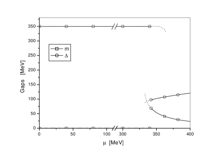
Figure 1: The constituent quark mass $m$ vs $\mu$ and color gap $\Delta$ vs $\mu$ under local color neutrality constraint.

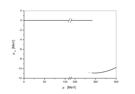
Figure 2: The behaviour of $\mu_{8}$ vs $\mu$ in the model (2) when local color neutrality is imposed.

IV Masses of the $\pi$- and $\sigma$-mesons

It turns out that the ${\cal S}^{(2)}_{\rm mixed}$ -part (22) of the effective action is composed from $\sigma(x)$, $\Delta^{s}_{2}(x)$ and $\Delta^{s*}_{2}(x)$ fields only. So it provides us with nondiagonal matrix elements $\Gamma_{\sigma X}$ ($X=\Delta^{s*}_{2},\Delta^{s}_{2}$) of the inverse propagator matrix of $\sigma$, $\Delta^{s*}_{2}$, and $\Delta^{s}_{2}$. Moreover, each term in ${\cal S}^{(2)}_{\rm mixed}$ is proportional to $\Delta$ or $\Delta^{*}$ as well as to the constituent quark mass $m$ (see Appendix). Hence, in the color symmetric phase ($\Delta=0$) there is no mixing between $\sigma$-meson and diquark $\Delta^{s}_{2}$ at all. The parameter $m$ is small (or even equals zero if $m_{0}=0$) in the 2SC phase, so we ignore for simplicity the $\sigma$-$\Delta^{s}_{2}$ mixing effect in this phase, too. As a result, in order to get the masses of mesons we use only the effective action (20) which has the form ${\cal S}^{(2)}_{\rm mesons}={\cal S}^{(2)}_{\rm\sigma\sigma}+{\cal S}^{(2)}_{\rm\pi\pi}$, where

$${\cal S}^{(2)}_{\rm\sigma\sigma}\!\!\!\! \!\!=-\int d^{4}x\frac{\sigma^{2}}{4G}+\frac{i}{4}{\rm Tr}_{scfx}\left\{S_{11}\sigma S_{11}\sigma+2S_{12}\sigma S_{21}\sigma+S_{22}\sigma S_{22}\sigma\right\}\equiv$$ (32)

$$~{}~{}~{}~{}~{}~{}~{}~{}~{}~{}~{}~{}~{}~{}~{}~{}~{}~{}~{}~{}~{}\equiv-\frac{1}{2}\int d^{4}ud^{4}v~{}\sigma(u)\Gamma(u-v)\sigma(v),$$

$${\cal S}^{(2)}_{\rm\pi\pi}\!\!\!\! \!\!=-\int d^{4}x\frac{\pi^{2}_{a}}{4G}+\frac{i}{4}{\rm Tr}_{scfx}\left\{S_{11}(i\gamma^{5}\pi_{a}\tau_{a})S_{11}(i\gamma^{5}\pi_{b}\tau_{b})+2S_{12}(i\gamma^{5}\pi_{a}\tau_{a}^{t})S_{21}(i\gamma^{5}\pi_{b}\tau_{b})+\right.$$ (33)

$$\left.+S_{22}(i\gamma^{5}\pi_{a}\tau_{a}^{t})S_{22}(i\gamma^{5}\pi_{b}\tau_{b}^{t})\right\}\equiv-\frac{1}{2}\int d^{4}ud^{4}v~{}\pi_{k}(u)\Pi_{kl}(u-v)\pi_{l}(v).$$

In these formulae $\Gamma(x-y)$ is the inverse propagator of $\sigma$-mesons, and $\Pi_{ab}(x-y)$ is the (diagonal) matrix of the inverse $\pi$-meson propagator. Evidently, that

$$\Gamma(x-y)=-\frac{\delta^{2}{\cal S}^{(2)}_{\sigma\sigma}}{\delta\sigma(y)\delta\sigma(x)},~{}~{}~{}~{}~{}~{}\Pi_{ab}(x-y)=-\frac{\delta^{2}{\cal S}^{(2)}_{\pi\pi}}{\delta\pi_{b}(y)\delta\pi_{a}(x)}.$$ (34)

Next, using in (32)-(33) the expressions (III)-(31) for the matrix elements $S_{ij}$, it is possible to obtain with the help of relations (34) the functions $\Gamma(x-y)$, $\Pi_{ab}(x-y)$, and then their momentum space representations, $\Gamma(p)$, $\Pi_{ab}(p)$, correspondingly. The zeros of these functions determine the particle and antiparticle dispersion laws, i.e. the relations between their energy and three-momenta. In the present paper, we are mainly interested in the investigation of the modification of meson and diquark masses in dense and cold color neutral quark matter. In this case, the particle mass is defined as the value of its energy in the rest frame, $\vec{p}=0$ (see, e.g., eky ; ruivo ), where the calculation of inverse propagators for $\sigma$- and $\pi$-mesons is significantly simplified. Indeed, in the rest frame it is possible to get:

$$\Pi_{ab}(p_{0})=\frac{\delta_{ab}}{2G}-8\delta_{ab}\int\frac{d^{3}q}{(2\pi)^{3}}\frac{E_{\Delta}^{+}E_{\Delta}^{-}+E^{+}E^{-}+\Delta^{2}}{E_{\Delta}^{+}E_{\Delta}^{-}}\frac{E_{\Delta}^{+}+E_{\Delta}^{-}}{(E_{\Delta}^{+}+E_{\Delta}^{-})^{2}-p_{0}^{2}}-$$

$$\qquad-16\delta_{ab}\int\frac{d^{3}q}{(2\pi)^{3}}\frac{\theta(E-\breve{\mu})E}{4E^{2}-p_{0}^{2}}\equiv\delta_{ab}\Pi(p_{0}),$$ (35)

$$\Gamma(p_{0})=\Gamma_{0}(p_{0}^{2})+\Gamma_{1}(p_{0}^{2}),$$ (36)

$$\Gamma_{0}(p_{0}^{2})=\frac{1}{2G}-8\int\frac{d^{3}q}{(2\pi)^{3}}\,\frac{\vec{q}^{2}}{E^{2}}\,\frac{E_{\Delta}^{+}E_{\Delta}^{-}+E^{+}E^{-}+\Delta^{2}}{E_{\Delta}^{+}E_{\Delta}^{-}}\,\frac{E_{\Delta}^{+}+E_{\Delta}^{-}}{(E_{\Delta}^{+}+E_{\Delta}^{-})^{2}-p_{0}^{2}}-16\int\frac{d^{3}q}{(2\pi)^{3}}\,\frac{\vec{q}^{2}}{E}\,\frac{\theta(E-\breve{\mu})}{4E^{2}-p_{0}^{2}},$$ (37)

$$\Gamma_{1}(p_{0}^{2})=16\Delta^{2}m^{2}\int\frac{d^{3}q}{(2\pi)^{3}E^{2}}\,\left\{\frac{1}{E_{\Delta}^{+}[p_{0}^{2}-4(E_{\Delta}^{+})^{2}]}+\frac{1}{E_{\Delta}^{-}[p_{0}^{2}-4(E_{\Delta}^{-})^{2}]}\right\},$$ (38)

where the same notations as in (23) were used. The zeros of the functions (35), (36) give us the masses of $\pi$- and $\sigma$-mesons, respectively (see Fig. 3). We see that in the 2SC phase the masses of the sigma- and pi-meson are about 300 MeV. Moreover, the pion is a stable particle in this phase (only electroweak decay channels are allowed). This conclusion is supported by the following arguments. It is clear that the first and the second integrals in (35) are analytical functions in the whole complex $p_{0}^{2}$ plane, except the cuts $E_{\rm min}^{2}<p_{0}^{2}<\infty$ and $(2\breve{\mu})^{2}<p_{0}^{2}<\infty$, respectively (here $E_{\rm min}=\sqrt{(\bar{\mu}-m)^{2}+|\Delta|^{2}}+\sqrt{(\bar{\mu}+m)^{2}+|\Delta|^{2}}$ is the minimum of the expression $E_{\Delta}^{-}+E_{\Delta}^{+}$, which is taken at the point $|\vec{p}|=0$). Evidently, $E_{\rm min}$ corresponds to the threshold for the pion decay into a red-green quark-antiquark pair, whereas $2\breve{\mu}$ corresponds to the threshold for the pion decay into a blue quark-antiquark pair. It is easily seen from Fig. 3 that in the 2SC phase the pion mass is less than the values of these two thresholds. Because there are no other singularities in (35) corresponding to different channels of the pion decay, we can conclude that in the 2SC phase the pion is a stable particle.

The neglection of the mixing between the $\sigma$-meson and $\Delta^{s}_{2}$-scalar diquark also results in a stable $\sigma$-meson. However, if the mixing is taken into account, then in the 2SC phase the $\sigma$-meson is a resonance, decaying into a pair of quarks, whose width is a rather small quantity, i.e. about 30 MeV (see Appendix).

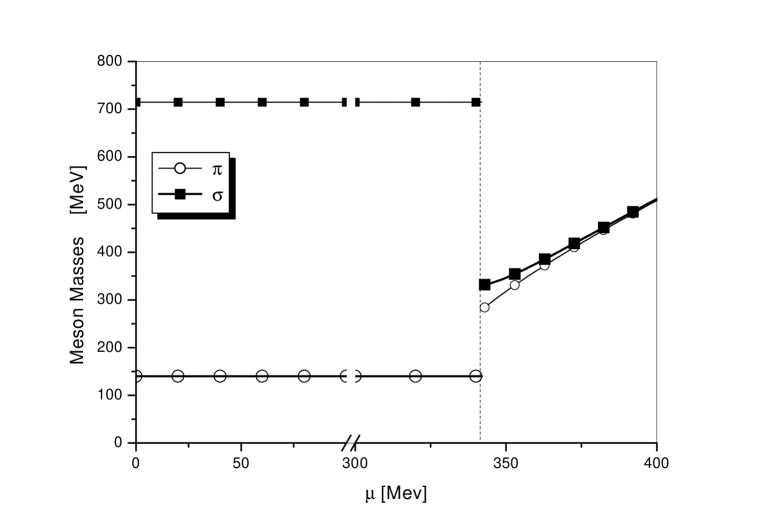
Figure 3: The masses of the $\sigma$-meson and pion as functions of $\mu$, when mixing of $\sigma$ and $\Delta^{s}_{2}$ is neglected.

V Masses of scalar diquarks

As in the previous section, we will ignor for simplicity the term ${\cal S}^{(2)}_{\rm mixed}$ (22), which mixes $\sigma$ and $\Delta^{s*}_{2},\Delta^{s}_{2}$ diquarks, in the effective action (19). In this case, in order to obtain the masses of diquarks, we need to analyze the term ${\cal S}^{(2)}_{\rm diquarks}$ (21) only. It can be easily presented in the following form

$${\cal S}^{(2)}_{\rm diquarks}=\sum_{A=2,5,7}\Big{\{}{\cal S}^{(2)}_{\rm s~{}AA}+{\cal S}^{(2)}_{\rm p~{}AA}\Big{\}},$$ (39)

where labels $s,p$ denote the contributions from scalar- and pseudo-scalar diquark fields, correspondingly, and

$${\cal S}^{(2)}_{\rm s~{}AA}\!\!\!\! \!\!=-\int d^{4}x\frac{\Delta^{s}_{A}\Delta^{s*}_{A}}{4H_{s}}+\frac{i}{2}{\rm Tr}_{scfx}\left\{S_{11}i\Delta^{s}_{A}\gamma^{5}\tau_{2}\lambda_{A}S_{22}i\Delta^{s*}_{A}\gamma^{5}\tau_{2}\lambda_{A}\right\},$$ (40)

$${\cal S}^{(2)}_{\rm p~{}AA}\!\!\!\! \!\!=-\int d^{4}x\frac{\Delta^{p}_{A}\Delta^{p*}_{A}}{4H_{p}}+\frac{i}{2}{\rm Tr}_{scfx}\left\{S_{11}\Delta^{p}_{A}\tau_{2}\lambda_{A}S_{22}\Delta^{p*}_{A}\tau_{2}\lambda_{A}\right\},$$ (41)

for fixed $A=5,7$, and

$${\cal S}^{(2)}_{\rm s~{}22}\!\!\!\! \!\!=-\int d^{4}x\frac{\Delta^{s}_{2}\Delta^{s*}_{2}}{4H_{s}}+\frac{i}{4}{\rm Tr}_{scfx}\left\{S_{12}i\Delta^{s*}_{2}\gamma^{5}\tau_{2}\lambda_{2}S_{12}i\Delta^{s*}_{2}\gamma^{5}\tau_{2}\lambda_{2}+\right.$$ (42)

$$\left.~{}~{}~{}~{}~{}~{}~{}~{}+2S_{11}i\Delta^{s}_{2}\gamma^{5}\tau_{2}\lambda_{2}S_{22}i\Delta^{s*}_{2}\gamma^{5}\tau_{2}\lambda_{2}+S_{21}i\Delta^{s}_{2}\gamma^{5}\tau_{2}\lambda_{2}S_{21}i\Delta^{s}_{2}\gamma^{5}\tau_{2}\lambda_{2}\right\},$$

$${\cal S}^{(2)}_{\rm p~{}22}\!\!\!\! \!\!=-\int d^{4}x\frac{\Delta^{p}_{2}\Delta^{p*}_{2}}{4H_{p}}+\frac{i}{4}{\rm Tr}_{scfx}\left\{S_{12}\Delta^{p*}_{2}\tau_{2}\lambda_{2}S_{12}\Delta^{p*}_{2}\tau_{2}\lambda_{2}+\right.$$ (43)

$$\left.~{}~{}~{}~{}~{}~{}~{}~{}~{}~{}~{}~{}~{}~{}+2S_{11}\Delta^{p}_{2}\tau_{2}\lambda_{2}S_{22}\Delta^{p*}_{2}\tau_{2}\lambda_{2}+S_{21}\Delta^{p}_{2}\tau_{2}\lambda_{2}S_{21}\Delta^{p}_{2}\tau_{2}\lambda_{2}\right\}.$$

It follows from (39)-(43) that there is no mixing between scalar- and pseudo-scalar diquarks. Moreover, scalar diquarks (or pseudo-scalar ones), as such, are not mixed to one another. Starting from the above formulae, we will find the inverse propagators of diquarks which migth be introduced by the following way ($A=2,5,7$):

$${\cal S}^{(2)}_{s~{}AA}=-\frac{1}{2}\sum_{X,Y}\int d^{4}ud^{4}v~{}X(u)\Gamma^{As}_{XY}(u-v)Y(v),$$ (44)

$${\cal S}^{(2)}_{p~{}AA}=-\frac{1}{2}\sum_{P,Q}\int d^{4}ud^{4}v~{}P(u)\Gamma^{Ap}_{PQ}(u-v)Q(v),$$ (45)

where (for each fixed value of $A$) $X(x),Y(x)=\Delta^{s}_{A}(x),\Delta^{s*}_{A}(x)$, $P(x),Q(x)=\Delta^{p}_{A}(x),\Delta^{p*}_{A}(x)$ and $\Gamma^{As}_{XY}(z)$ or $\Gamma^{Ap}_{PQ}(z)$ are matrix elements of the $2\times 2$ inverse propagator matrix for $\Delta^{s}_{A}(x),\Delta^{s*}_{A}(x)$- or $\Delta^{p}_{A}(x),\Delta^{p*}_{A}(x)$-fields, respectively. Given diquark propagators, it is possible then to obtain the masses of diquarks.

V.1 Scalar diquarks in the 2SC phase ($\Delta\neq 0$, $\mu_{8}\neq 0$)

In the present section, using (44) for different $A=2,5,7$, we will study step-by-step the masses of scalar diquark excitations in the 2SC phase of the model (2), when the color neutrality condition is taken into account. Let us begin with the $\Delta^{s}_{5}$ -$\Delta^{s*}_{5}$ diquark sector. It follows from (44) at $A=5$ that

$$\Gamma^{5s}_{XY}(x-y)=-\frac{\delta^{2}{\cal S}^{(2)}_{s~{}55}}{\delta Y(y)\delta X(x)}$$ (46)

(recall, $X,Y=\Delta^{s}_{5}(x),\Delta^{s*}_{5}(x)$ in the case under consideration). Note also that $\Gamma^{5s}(z)$ is a symmetric matrix, i.e. $\Gamma^{5s}_{XY}(z)=\Gamma^{5s}_{YX}(-z)$. It is clear from (44) and (46) that $\Gamma^{5s}_{\Delta^{s}_{5}\Delta^{s}_{5}}(z)=\Gamma^{5s}_{\Delta^{s*}_{5}\Delta^{s*}_{5}}(z)=0$, and this matrix has nonzero elements of the form (in the momentum space representation):

$$\Gamma^{5s}_{\Delta^{s*}_{5}\Delta^{s}_{5}}(p)=\frac{1}{4H_{s}}-i{\rm Tr}_{sc}\int\frac{d^{4}q}{(2\pi)^{4}}\left\{S_{11}(q+p)i\gamma^{5}\lambda_{5}S_{22}(q)i\gamma^{5}\lambda_{5}\right\},$$ (47)

$$\Gamma^{5s}_{\Delta^{s}_{5}\Delta^{s*}_{5}}(p)=\frac{1}{4H_{s}}-i{\rm Tr}_{sc}\int\frac{d^{4}q}{(2\pi)^{4}}\left\{S_{22}(q+p)i\gamma^{5}\lambda_{5}S_{11}(q)i\gamma^{5}\lambda_{5}\right\},$$ (48)

where the Fourier-transformed expressions $S_{11}(q)$, $S_{22}(q)$ can be easily determined from (III), (29). It follows from (47)-(48) that $\Gamma^{5s}_{\Delta^{s*}_{5}\Delta^{s}_{5}}(-p)=$ $\Gamma^{5s}_{\Delta^{s}_{5}\Delta^{s*}_{5}}(p)$. Since we are interested in diquark masses, it is necessary to use the rest frame in (47)-(48), i.e. $p=(p_{0},0,0,0)$ (see also eky ; ruivo ). In this case the calculation of matrix elements (47)-(48) is greatly simplified, and mass excitations are connected with the zeros of the quantity ${\rm det}~{}\Gamma^{5s}(p_{0})$ in the $p_{0}^{2}$-plane. So, we have

$$\Gamma^{5s}_{\Delta^{s*}_{5}\Delta^{s}_{5}}(p_{0})=\frac{1}{4H_{s}}-4i\int\frac{d^{4}q}{(2\pi)^{4}}\left\{\frac{q_{0}+E^{+}}{(p_{0}+q_{0}+\breve{E}^{+})(q_{0}^{2}-(E_{\Delta}^{+})^{2})}+\frac{q_{0}-E^{-}}{(p_{0}+q_{0}-\breve{E}^{-})(q_{0}^{2}-(E_{\Delta}^{-})^{2})}\right\}.$$ (49)

The $p_{0},q_{0}$-dependency in the integrand of (49) is presented in an evident form. Other quantities in (49), such as $E^{\pm}$ etc, depend on $|\vec{q}|$ only. The expression (49) is valid both for $\Delta=0$ and $\Delta\neq 0$. For the case $\Delta\neq 0$, i.e. in the color superconducting phase, it is possible to use the gap equation (24) in order to eliminate the coupling constant $H_{s}$ from this formula. In this way we find:

$$\Gamma^{5s}_{\Delta^{s*}_{5}\Delta^{s}_{5}}(p_{0})=4i(p_{0}-3\mu_{8})\int\frac{d^{4}q}{(2\pi)^{4}}\left\{\frac{1}{(p_{0}+q_{0}+\breve{E}^{+})(q_{0}^{2}-(E_{\Delta}^{+})^{2})}+\frac{1}{(p_{0}+q_{0}-\breve{E}^{-})(q_{0}^{2}-(E_{\Delta}^{-})^{2})}\right\}\equiv$$

$$~{}~{}~{}~{}~{}~{}~{}\equiv 2(p_{0}-3\mu_{8})H(p_{0}),~{}~{}~{}~{}~{}~{}~{}~{}~{}~{}~{}~{}~{}\Gamma^{5s}_{\Delta^{s}_{5}\Delta^{s*}_{5}}(p_{0})=-2(p_{0}+3\mu_{8})H(-p_{0}).$$ (50)

The last equation in (50) is due to the relation $\Gamma^{5s}_{\Delta^{s*}_{5}\Delta^{s}_{5}}(-p_{0})=$ $\Gamma^{5s}_{\Delta^{s}_{5}\Delta^{s*}_{5}}(p_{0})$. Recall, in (50) $q_{0}+p_{0}$ and $q_{0}$ are shorthands for $(p_{0}+q_{0})+i\varepsilon\cdot{\rm sign}(p_{0}+q_{0})$ and $q_{0}+i\varepsilon\cdot{\rm sign}(q_{0})$, where $\varepsilon\to 0_{+}$ (see also comment after formula (25)). Performing in (50) the $q_{0}$-integration, one obtains

$$H(p_{0})=\int\frac{d^{3}q}{(2\pi)^{3}}\left\{\frac{\theta(\breve{E}^{+})}{(p_{0}+\breve{E}^{+}+E_{\Delta}^{+})E_{\Delta}^{+}}\!\!\right. + \!\!\frac{\theta(-\breve{E}^{+})}{(p_{0}+\breve{E}^{+}-E_{\Delta}^{+})E_{\Delta}^{+}}+\frac{\theta(\breve{E}^{-})}{(p_{0}-\breve{E}^{-}-E_{\Delta}^{-})E_{\Delta}^{-}}+$$ (51)

$$\left.+\frac{\theta(-\breve{E}^{-})}{(p_{0}-\breve{E}^{-}+E_{\Delta}^{-})E_{\Delta}^{-}}\right\}.$$

Now, with the help of (50) one easily gets the expression for the determinant of the inverse propagator matrix $\Gamma^{5s}(p_{0})$ in the rest frame:

$${\rm det}\Gamma^{5s}(p_{0})=\Gamma^{5s}_{\Delta^{s*}_{5}\Delta^{s}_{5}}(p_{0})\Gamma^{5s}_{\Delta^{s}_{5}\Delta^{s*}_{5}}(p_{0})\equiv-4(p_{0}^{2}-9\mu_{8}^{2})H(p_{0})H(-p_{0}).$$ (52)

The diquark squared mass spectrum in the $\Delta^{s}_{5}$-sector of the theory is defined by zeros of the det$\Gamma^{5s}(p_{0})$ in the $p_{0}^{2}$-plane. Evidently, the point $p_{0}^{2}=9\mu_{8}^{2}$ is the solution of the equation det$\Gamma^{5s}(p_{0})=0$. Let us suppose that some nonzero point $p_{0}=-M^{s}_{D}$ is the zero of the function $H(p_{0})$, i.e. $H(-M^{s}_{D})=0$. Then, at $p_{0}=M^{s}_{D}$ the determinant (52) is also equal to zero, so the point $p_{0}^{2}=(M^{s}_{D})^{2}$ is another zero of ${\rm det}\overline{\Gamma^{5s}}(p_{0})$ in the $p_{0}^{2}$-plane, and the second bosonic excitation of this sector has nonzero mass $M^{s}_{D}$. It follows from (51) and (26) that $H(p_{0})$ is proportional to $\langle Q_{8}\rangle$ at the point $p_{0}=3\mu_{8}$. Namely, $H(3\mu_{8})\equiv-\langle Q_{8}\rangle\big{/}(4\Delta^{2})$. Since $\langle Q_{8}\rangle$ is zero due to the constraint (26), we may conclude that $M^{s}_{D}=3|\mu_{8}|$. Hence, in the $\Delta^{s}_{5}$-sector of the model there are two real bosonic excitations with equal masses $M^{s}_{D}\equiv 3|\mu_{8}|$.

The similar is true for the $\Delta^{s}_{7}$-sector of the model, so in the whole $\Delta^{s}_{5},\Delta^{s}_{7}$-sector of the NJL model that is under the color neutrality constraint there are four massive scalar excitations with equal masses $M^{s}_{D}\equiv 3|\mu_{8}|$. These particles form two real antidoublets of the $\rm SU_{c}(2)$-group, or one complex antidoublet.

Consider now the diquark excitations of the 2SC ground state in the $\Delta^{s}_{2}$-$\Delta^{s*}_{2}$ sector of the model. In this case, the matrix $\Gamma^{2s}(p_{0})$ (the momentum representation for the inverse propagator matrix at $\vec{p}=0$, i.e. in the rest frame) has the following structure:

$$\Gamma^{2s}_{\Delta^{s}_{2}\Delta^{s}_{2}}(p_{0}) = \Gamma^{2s}_{\Delta^{s*}_{2}\Delta^{s*}_{2}}(p_{0})=4\Delta^{2}I_{0}(p_{0}^{2}),~{}~{}~{}~{}~{}~{}~{}\Gamma^{2s}_{\Delta^{s}_{2}\Delta^{s*}_{2}}(p_{0})=\Gamma^{2s}_{\Delta^{s*}_{2}\Delta^{s}_{2}}(-p_{0})=$$ (53)

$$= (4\Delta^{2}-2p_{0}^{2})I_{0}(p_{0}^{2})+4p_{0}I_{1}(p_{0}^{2}),$$

where

$$I_{0}(p_{0}^{2})=\int\frac{d^{3}q}{(2\pi)^{3}}\frac{1}{E_{\Delta}^{+}[4(E_{\Delta}^{+})^{2}-p_{0}^{2}]}+\int\frac{d^{3}q}{(2\pi)^{3}}\frac{1}{E_{\Delta}^{-}[4(E_{\Delta}^{-})^{2}-p_{0}^{2}]},$$ (54)

$$I_{1}(p_{0}^{2})=\int\frac{d^{3}q}{(2\pi)^{3}}\frac{E^{+}}{E_{\Delta}^{+}[4(E_{\Delta}^{+})^{2}-p_{0}^{2}]}-\int\frac{d^{3}q}{(2\pi)^{3}}\frac{E^{-}}{E_{\Delta}^{-}[4(E_{\Delta}^{-})^{2}-p_{0}^{2}]}.$$ (55)

The mass spectrum is defined by the equation

$${\rm det}\Gamma^{2s}(p_{0})\equiv 4p_{0}^{2}\big{\{}(p_{0}^{2}-4\Delta^{2})I_{0}^{2}(p_{0}^{2})-4I_{1}^{2}(p_{0}^{2})\big{\}}=0.$$ (56)

In the $p_{0}^{2}$-plane this equation has an evident zero, corresponding to a Nambu–Goldstone boson, $p_{0}^{2}=0$. Detailed investigation, similar to that from eky , shows that on the second Riemann sheet of $p_{0}^{2}$ there is another zero of (56) which corresponds to a heavy resonance. Its mass $M$ and width $\Gamma$ are depicted in the Fig. 4.

As a result, we conclude that in the 2SC phase there are four light real scalar diquark excitations with mass $3|\mu_{8}|$, and one Nambu–Goldstone boson, which appears due to a spontaneous breaking of the $\rm SU_{c}(2)\times U_{\lambda_{8}}(1)$ color symmetry down to $\rm SU_{c}(2)$. Moreover, a heavy scalar diquark resonance, which is an $\rm SU_{c}(2)$-singlet, is also presented in the mass spectrum of the model at $\mu>\mu_{c}=342$ MeV (see Fig. 4).

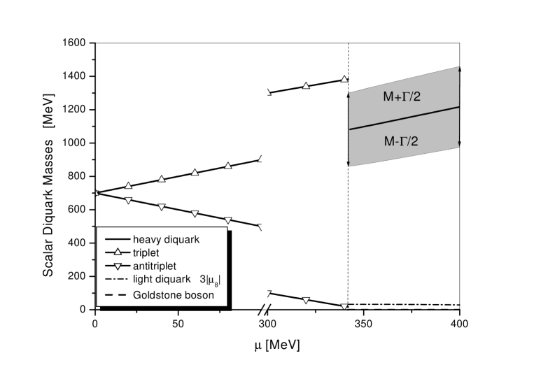
Figure 4: The masses of diquarks. At $\mu<\mu_{c}=342$ MeV, six diquark states are splitted into a (color)triplet of heavy states with mass $M_{\Delta^{*}}$ and an anti-triplet of light states with mass $M_{\Delta}$ (see (59)). In the 2SC phase ($\mu>\mu_{c}$), one observes the Numbu–Goldstone boson, four light diquarks with the mass $3|\mu_{8}|$, and a heavy singlet state with the mass $M$ (solid line). The shaded rectangular displays the width $\Gamma$ of the heavy singlet resonance; its upper border is half-width higher than the mass and the bottom border is half-width lower.

V.2 Scalar diquarks in the normal phase ($\Delta=0$, $\mu_{8}=0$)

In the $\rm SU_{c}(3)$-symmetric phase ($\mu<\mu_{c}$) the diquark gap $\Delta$ is zero and the three complex diquark fields $\Delta^{s}_{A}(x)$ ($A=2,5,7$) are not mixed with other fields in the second order effective action of the model. Moreover, at $\Delta=0$, as it is easily seen from the color neutrality constraint (26), we have $\mu_{8}=0$. So, in order to study the diquark masses, it is enough to consider, e.g., the $\Delta^{s}_{5}$-diquark sector. In this phase the determinant of the inverse propagator matrix $\Gamma^{5s}(p_{0})$ looks like (we use the rest frame, where $\vec{p}=0$)

$${\rm det}\Gamma^{5s}(p_{0})=\Gamma^{5s}_{\Delta^{s*}_{5}\Delta^{s}_{5}}(p_{0})\Gamma^{5s}_{\Delta^{s}_{5}\Delta^{s*}_{5}}(p_{0})=\Gamma^{5s}_{\Delta^{s*}_{5}\Delta^{s}_{5}}(p_{0})\Gamma^{5s}_{\Delta^{s*}_{5}\Delta^{s}_{5}}(-p_{0}),$$ (57)

where $\Gamma^{5s}_{\Delta^{s*}_{5}\Delta_{5}}(p_{0})$ is presented in (49). (Note, the last equality in formula (52) for ${\rm det}\Gamma^{5s}(p_{0})$ in the 2SC phase is based on the usage of a non trivial solution $\Delta\neq 0$ of the gap equation (24). So, in the normal $\rm SU_{c}(3)$-symmetric phase, where $\Delta=0$, it is not valid.) Taking into account the relation $m>\mu$ that is realized in the normal phase only (see Fig. 1), we see that $E\equiv\sqrt{\vec{q}^{2}+m^{2}}>\mu$ and, as a consequence, $E^{\pm}>0$ are fulfilled in this phase. So, one can easily integrate in (49) over $q_{0}$ and obtain the following expression that is suitable only for $\rm SU_{c}(3)$-symmetric phase:

$$\Gamma^{5s}_{\Delta^{s*}_{5}\Delta^{s}_{5}}(p_{0})=\frac{1}{4H_{s}}-16\int\frac{d^{3}q}{(2\pi)^{3}}\frac{E}{4E^{2}-(p_{0}+2\mu)^{2}}\equiv\frac{1}{4H_{s}}-F_{s}(\epsilon),$$ (58)

where $\epsilon=(p_{0}+2\mu)^{2}$. Clearly, the diquark mass spectrum is defined by the equation ${\rm det}\Gamma^{5s}(p_{0})=0$, or by zeros of (58), where the function $F_{s}(\epsilon)$ is analytical in the whole complex $\epsilon$-plane, except for the cut $4m^{2}<\epsilon$ along the real axis. (In general, $F_{s}(\epsilon)$ is defined on a complex Riemann surface which is to be described by several sheets. However, a direct numerical computation based on eq. (58) gives its values on the first sheet only (we use the parameter set (27)). To find a value on the rest of the Riemann surface, a special procedure of continuation is needed.) The numerical analysis of (58) on the first Riemann sheet shows that the equation $\Gamma^{5s}_{\Delta^{s*}_{5}\Delta_{5}}(p_{0})=0$ has a root ($\epsilon_{0}$) on the real axis ($0<\epsilon_{0}<4m^{2}$), providing us with the following massive diquark modes which are the solutions of the eq. (57)

$$(M^{s}_{\Delta})^{2}=(1.998m-2\mu)^{2},~{}~{}~{}~{}~{}(M^{s}_{\Delta^{*}})^{2}=(1.998m+2\mu)^{2}.$$ (59)

We relate $M^{s}_{\Delta}$ in (59) to the mass of the diquark with the baryon number $B=2/3$ and $M^{s}_{\Delta^{*}}$ to the mass of the antidiquark with $B=-2/3$. (Qualitatively, a similar behavior of diquark and antidiquark masses vs. $\mu$ was obtained in ratti in the NJL model with two-colored quarks.) The difference between diquark and antidiquark masses in (59) is explained by the absence of a charge conjugation symmetry in the presence of a chemical potential.

Finally, due to the underling color $\rm SU(3)_{c}$ symmetry, the previous statement is valid also for $\Delta^{*}_{5},\Delta_{5}$ and $\Delta^{*}_{7},\Delta_{7}$. As a result, we have a color antitriplet of diquarks with the mass $M^{s}_{\Delta}$ (59) as well as a color triplet of antidiquarks with the mass $M^{s}_{\Delta^{*}}$. The results of numerical computations are presented in Fig. 4 for $\mu<\mu_{c}=342$ MeV.

Recall that in our analysis, we have used the constraint $H_{s}=3G/4$, thereby fixing the constant $H_{s}$ through $G$. It is useful, however, to discuss now the influence of $H_{s}$ on diquark masses. Indeed, it is clear from (58) that the root $\epsilon_{0}$ lies inside the interval $0<\epsilon_{0}<4m^{2}$ only if $H_{s}^{*}<H_{s}<H_{s}^{**}$, where $H_{s}^{*}$ and $H_{s}^{**}$ are defined by

$$H_{s}^{*} \equiv \frac{1}{4F_{s}(4m^{2})}=\frac{\pi^{2}}{4\left[\Lambda\sqrt{m^{2}+\Lambda^{2}}+m^{2}\ln((\Lambda+\sqrt{m^{2}+\Lambda^{2}})/m)\right]},$$

$$H_{s}^{**} \equiv \frac{1}{4F_{s}(0)}=\frac{\pi^{2}}{4\left[\Lambda\sqrt{m^{2}+\Lambda^{2}}-m^{2}\ln((\Lambda+\sqrt{m^{2}+\Lambda^{2}})/m)\right]}=\frac{3mG}{2(m-m_{0})}.$$ (60)

In this case, there are stable diquarks and antidiquarks in the color symmetric phase. The behavior of their masses qualitatively resembles that given by eqs. (59). For a rather weak interaction in the diquark channel ($H_{s}<H_{s}^{*}$), $\epsilon_{0}$ runs onto the second Riemann sheet, and unstable diquark modes (resonances) appear. Unlike this, a sufficiently strong interaction in the diquark channel ($H_{s}>H_{s}^{**}$) pushes $\epsilon_{0}$ towards the negative semi-axis, i. e. $(p_{0}+2\mu)^{2}<0$. The latter indicates a tachyon singularity in the diquark propagator, evidencing that the $\rm SU_{c}(3)$-color symmetric ground state is not stable. Indeed, at a very large $H_{s}$, as it has been shown in ek at $H_{p}=0$, the color symmetry is spontaneously broken even at a vanishing chemical potential. We guess that this result remains true at rather small values of $H_{p}$ ($H_{p}<H_{s}$) as well, justifying the above mentioned tachyon singularity of the diquark propagator.

VI Masses of pseudo-scalar diquarks

It is clear from (39) that in the framework of the NJL model (2) pseudo-scalar diquarks are not mixing with each other as well as with meson- and scalar diquark fields. So, to get their masses, we will start from the general expression (45) for the inverse propagator matrices of pseudo-scalar diquarks.

VI.1 Pseudo-scalar diquarks in the 2SC phase ($\Delta\neq 0$, $\mu_{8}\neq 0$)

In the 2SC phase there is an $\rm SU(2)_{c}$ symmetry between $\Delta^{p}_{5}$-$\Delta^{p*}_{5}$ and $\Delta^{p}_{7}$-$\Delta^{p*}_{7}$ sectors, so it is enough to study an inverse propagator, e.g., in one of these sectors. For $A=5$ it follows from (45) that

$$\Gamma^{5p}_{PQ}(x-y)=-\frac{\delta^{2}{\cal S}^{(2)}_{p~{}55}}{\delta Q(y)\delta P(x)},$$ (61)

where $P(x),Q(x)$ = $\Delta^{p}_{5}(x),\Delta^{p*}_{5}(x)$. Further, using the evident expression (41) for ${\cal S}^{(2)}_{p~{}55}$, one can obtain the matrix elements (61) in the rest frame, $\vec{p}=0$, of the momentum space representation

$$\Gamma^{5p}_{\Delta^{p*}_{5}\Delta^{p}_{5}}(p_{0})=\frac{1}{4H_{p}}+4\int\frac{d^{3}q}{(2\pi)^{3}}\left\{\frac{m^{2}}{E^{2}}\Big{[}\frac{(\breve{E}^{-}-p_{0}+E^{+})\theta(-\breve{E}^{-})}{(p_{0}-\breve{E}^{-})^{2}-(E_{\Delta}^{+})^{2}}-\frac{E^{+}-E_{\Delta}^{+}}{2(p_{0}-\breve{E}^{-}-E_{\Delta}^{+})E_{\Delta}^{+}}-\right.$$

$$~{}~{}~{}~{}~{}~{}~{}~{}-\frac{(\breve{E}^{+}+p_{0}+E^{-})\theta(\breve{E}^{+})}{(p_{0}+\breve{E}^{+})^{2}-(E_{\Delta}^{-})^{2}}+\frac{E^{-}+E_{\Delta}^{-}}{2(p_{0}+\breve{E}^{+}-E_{\Delta}^{-})E_{\Delta}^{-}}\Big{]}+\frac{\vec{q}^{2}}{E^{2}}\Big{[}\frac{(E^{+}-\breve{E}^{+}-p_{0})\theta(\breve{E}^{+})}{(p_{0}+\breve{E}^{+})^{2}-(E_{\Delta}^{+})^{2}}-$$

$$~{}~{}~{}~{}~{}~{}~{}~{}\left.-\frac{E^{+}-E_{\Delta}^{+}}{2(p_{0}+\breve{E}^{+}-E_{\Delta}^{+})E_{\Delta}^{+}}+\frac{(\breve{E}^{-}-p_{0}-E^{-})\theta(-\breve{E}^{-})}{(p_{0}-\breve{E}^{-})^{2}-(E_{\Delta}^{-})^{2}}+\frac{E^{-}+E_{\Delta}^{-}}{2(p_{0}-\breve{E}^{-}-E_{\Delta}^{-})E_{\Delta}^{-}}\Big{]}\right\},$$ (62)

$\Gamma^{5p}_{\Delta^{p}_{5}\Delta^{p*}_{5}}(p)=\Gamma^{5p}_{\Delta^{p*}_{5}\Delta^{p}_{5}}(-p)$, and $\Gamma^{5p}_{\Delta^{p}_{5}\Delta^{p}_{5}}(p)=$ $\Gamma^{5p}_{\Delta^{p*}_{5}\Delta^{p*}_{5}}(p)=0$. Let $\frac{1}{4H_{p}}=\frac{1}{4H_{s}}+\eta$. Then, using for $\frac{1}{4H_{s}}$ the gap equation (24) (recall, in the 2SC phase $\Delta\neq 0$), we obtain from (62) (transforming the multiplier before the second square bracket in (62) as $\vec{q}^{2}/E^{2}=1-m^{2}/E^{2}$):

$$\Gamma^{5p}_{\Delta^{p*}_{5}\Delta^{p}_{5}}(p_{0})=\eta+2(p_{0}-3\mu_{8})H(p_{0})+m^{2}\widetilde{H}(p_{0}),$$ (63)

where $H(p_{0})$ is defined in (51). Since in the 2SC phase $m<<\Delta$ (or $m$ even a zero if $m_{0}=0$), we ignore the last term in (63) (due to this reason an explicit form of $\widetilde{H}(p_{0})$ is not presented here) and obtain in this way the following expression for the determinant of the matrix $\Gamma^{5p}(p_{0})$:

$${\rm det}\Gamma^{5p}(p_{0})=\Gamma^{5p}_{\Delta^{p*}_{5}\Delta^{p}_{5}}(p_{0})\Gamma^{5p}_{\Delta^{p}_{5}\Delta^{p*}_{5}}(p_{0})=\Gamma^{5p}_{\Delta^{p*}_{5}\Delta^{p}_{5}}(p_{0})\Gamma^{5p}_{\Delta^{p*}_{5}\Delta^{p}_{5}}(-p_{0})=$$

$$\Big{[}\eta+2(p_{0}-3\mu_{8})H(p_{0})\Big{]}\Big{[}\eta-2(p_{0}+3\mu_{8})H(-p_{0})\Big{]}\approx\Big{[}\eta+2(p_{0}-3\mu_{8})^{2}\beta\Big{]}\Big{[}\eta+2(p_{0}+3\mu_{8})^{2}\beta\Big{]},$$ (64)

where $\beta=dH(p_{0})/dp_{0}|_{p_{0}=3\mu_{8}}$. In the last relation in (64) we have expanded the function $H(p_{0})$ into a Taylor-series of $p_{0}$ at the point $p_{0}=3\mu_{8}$, and took into account that $H(3\mu_{8})$ equals zero under the color neutrality constraint (see the end of section V.1). Solving in this approximation the equation ${\rm det}\Gamma^{5p}(p_{0})=0$, it is possible to find pseudo-scalar diquark excitations with two different masses:

$$M^{p}_{D1}=\Big{|}~{}3\mu_{8}+\sqrt{-\eta/(2\beta)}~{}\Big{|},~{}~{}~{}~{}~{}~{}~{}~{}~{}~{}~{}~{}~{}~{}M^{p}_{D2}=\sqrt{-\eta/(2\beta)}-3\mu_{8}.$$ (65)

Since $\beta<0$ (as is easily seen from (51)), we conclude from formulae (65) that at $\eta>0$ both $M^{p}_{D1}$ and $M^{p}_{D2}$ are real (positive) quantities, suggesting that these pseudo-scalars are stable particles at $H_{p}\leq H_{s}$. (The case $\eta<0$, which corresponds to an unstable 2SC ground state, will be discussed in details below, after (70).) The similar is true in the $\Delta^{p}_{7}$-$\Delta^{p*}_{7}$ sector of the model, so in the whole $\Delta^{p}_{5}$-$\Delta^{p*}_{5}$, $\Delta^{p}_{7}$-$\Delta^{p*}_{7}$ sector of the NJL model which is under the color neutrality constraint there are four massive pseudoscalar excitations: two of them form an $\rm SU_{c}(2)$-antidoublet with mass $M^{p}_{D1}$, another two particles form an $\rm SU_{c}(2)$-antidoublet with mass $M^{p}_{D2}$.

Now let us consider the 2SC ground state excitations in the $\Delta^{p}_{2}$-$\Delta^{p*}_{2}$ sector. In this case, starting from the effective action (43), it is possible to obtain the inverse propagator matrix $\Gamma^{2p}$ which is defined by the relation (45). In the rest frame, where $p=(p_{0},0,0,0)$, its Fourier-transformed matrix elements look like

$$\Gamma^{2p}_{\Delta^{p*}_{2}\Delta^{p}_{2}}(p_{0})=\frac{1}{4H_{p}}-4i\int\frac{d^{4}q}{(2\pi)^{4}}\left\{\frac{2m^{2}}{E^{2}}\cdot\frac{p_{0}+q_{0}-E^{+}}{(p_{0}+q_{0})^{2}-(E_{\Delta}^{+})^{2}}\cdot\frac{q_{0}-E^{-}}{q_{0}^{2}-(E_{\Delta}^{-})^{2}}+\right.$$

$$~{}~{}~{}~{}~{}\left.+\frac{\vec{q}^{2}}{E^{2}}\Big{[}\frac{p_{0}+q_{0}-E^{+}}{(p_{0}+q_{0})^{2}-(E_{\Delta}^{+})^{2}}\cdot\frac{q_{0}+E^{+}}{q_{0}^{2}-(E_{\Delta}^{+})^{2}}+\frac{p_{0}+q_{0}+E^{-}}{(p_{0}+q_{0})^{2}-(E_{\Delta}^{-})^{2}}\cdot\frac{q_{0}-E^{-}}{q_{0}^{2}-(E_{\Delta}^{-})^{2}}\Big{]}\right\},$$ (66)

$$\Gamma^{2p}_{\Delta^{p}_{2}\Delta^{p*}_{2}}(p_{0})=\Gamma^{2p}_{\Delta^{p*}_{2}\Delta^{p}_{2}}(-p_{0}),~{}~{}~{}~{}~{}~{}~{}~{}~{}~{}~{}~{}\Gamma^{2p}_{\Delta^{p}_{2}\Delta^{p}_{2}}(p_{0})=\Gamma^{2p}_{\Delta^{p*}_{2}\Delta^{p*}_{2}}(p_{0})=-4\Delta^{2}\mathbb{P}(p_{0}),$$

$$\mathbb{P}(p_{0})=\int\frac{d^{4}q}{i(2\pi)^{4}}\left\{\frac{2m^{2}}{E^{2}}\cdot\frac{1}{(p_{0}+q_{0})^{2}-(E_{\Delta}^{+})^{2}}\cdot\frac{1}{q_{0}^{2}-(E_{\Delta}^{-})^{2}}+\right.$$

$$\left.+\frac{\vec{q}^{2}}{E^{2}}\Big{[}\frac{1}{(p_{0}+q_{0})^{2}-(E_{\Delta}^{+})^{2}}\cdot\frac{1}{q_{0}^{2}-(E_{\Delta}^{+})^{2}}+\frac{1}{(p_{0}+q_{0})^{2}-(E_{\Delta}^{-})^{2}}\cdot\frac{1}{q_{0}^{2}-(E_{\Delta}^{-})^{2}}\Big{]}\right\}.$$ (67)

Using in (66)-(67) the substitution $\frac{1}{4H_{p}}=\frac{1}{4H_{s}}+\eta$ and then eliminating the coupling constant $H_{s}$ in favor of another model parameters (with the help of the gap equation (24)), we obtain after $q_{0}$-integrations:

$$\mathbb{P}(p_{0})=I_{0}(p_{0}^{2})+m^{2}A(p_{0}),~{}~{}~{}~{}~{}\Gamma^{2p}_{\Delta^{p*}_{2}\Delta^{p}_{2}}(p_{0})=\eta+(4\Delta^{2}-2p_{0}^{2})I_{0}(p_{0}^{2})+4p_{0}I_{1}(p_{0}^{2})+m^{2}B(p_{0}),$$ (68)

where $I_{0}(p_{0}^{2})$ and $I_{1}(p_{0}^{2})$ are presented in (54) and (55), respectively. The last terms in each of expressions (68) are proportional to $m^{2}$. In the 2SC phase the constituent quark mass $m$ is a vanishingly small quantity (or it is exactly zero if the current quark mass vanishes, $m_{0}=0$) as compared with $\Delta$, etc (see Fig. 1), so we will ignore the contributions of these terms in the matrix elements (66)-(67). Thus, there is no need to have explicit expressions for the functions $A(p_{0})$ and $B(p_{0})$ from (68). In this approximation the determinant of the inverse propagator matrix $\Gamma^{2p}(p_{0})$ looks like:

$${\rm det}\Gamma^{2p}(p_{0})=\Gamma^{2p}_{\Delta^{p*}_{2}\Delta^{p}_{2}}(p_{0})\Gamma^{2p}_{\Delta^{p}_{2}\Delta^{p*}_{2}}(p_{0})-\Gamma^{2p}_{\Delta^{p}_{2}\Delta^{p}_{2}}(p_{0})\Gamma^{2p}_{\Delta^{p*}_{2}\Delta^{p*}_{2}}(p_{0})=$$

$$=\Big{[}\eta-2p_{0}^{2}I_{0}(p_{0}^{2})\Big{]}\Big{[}\eta-2(p_{0}^{2}-4\Delta^{2})I_{0}(p_{0}^{2})\Big{]}-16p_{0}^{2}I^{2}_{1}(p_{0}^{2}).$$ (69)

Obviously, at $\eta=0$ the equation ${\rm det}\overline{\Gamma^{2p}}(p_{0})=0$ coincides with eq. (56) and has the same solutions. The first one, $p_{0}^{2}=0$, corresponds to a stable massless pseudo-scalar excitation, the second one lies in the second Riemann sheet of the variable $p_{0}^{2}$. So it is a heavy pseudo-scalar resonance and its mass and width are represented in the Fig. 4. At small nonzero values of $\eta$ it is reasonable to suppose that the equation ${\rm det}\overline{\Gamma^{2p}}(p_{0})=0$ has a root lying on the second Riemann sheet of $p_{0}^{2}$ as well. It might be considered as a weak disturbance of the resonance solution of this equation at $\eta=0$, so its mass and width behavior vs $\mu$ are qualitatively the same as on the Fig. 4. Another solution of this equation, $p_{0}^{2}=(M_{D3}^{p})^{2}$, should not be significantly different from the solution $p_{0}^{2}=0$ at $\eta=0$. So, in searching of $(M_{D3}^{p})^{2}$, one can expand the expression (69) into a Taylor-series of $p_{0}^{2}=0$:

$$(M_{D3}^{p})^{2}=\frac{\eta(\eta+8\Delta^{2}a)}{16b^{2}+2a(\eta+8\Delta^{2}a)+2\eta(a-4\Delta^{2}a^{\prime})},$$ (70)

where $a=I_{0}(0)$, $b=I_{1}(0)$, $a^{\prime}=I_{0}^{\prime}(0)$. Note that both the heavy resonance and stable excitation with mass squared (70) in the pseudo-scalar diquark channel are singlets with respect to $\rm SU_{c}(2)$. Since $a>0$, the expression (70) is a positive one at rather small and positive values of $\eta$. However, at sufficiently small, but negative values of $\eta$, it is a negative quantity, i.e. a tachyonic pseudo-diquark excitation appeared in the model. This fact indicates the instability of the 2SC ground state with $\langle\Delta^{s}_{2}(x)\rangle=\Delta$, $\langle\Delta^{s}_{5}(x)\rangle=0$, $\langle\Delta^{s}_{7}(x)\rangle=0$, and $\langle\Delta^{p}_{A}(x)\rangle=0$. Perhaps, in this case, i.e. at $H_{p}>H_{s}$, the phase with nonzero ground state expectation values of pseudo-scalar diquarks, $\langle\Delta^{p}_{A}(x)\rangle\neq 0$, should be realized.

As a result, we have shown that in the 2SC phase of the NJL model (2) there are five stable diquark excitations in the pseudo-scalar channel. They form a singlet as well as two antidoublets (in the case $H_{p}<H_{s}$) of the $\rm SU_{c}(2)$ group with masses presented in (70) and (65), correspondingly. Moreover, there is also a heavy resonance that is $\rm SU_{c}(2)$-singlet with mass about 1100 MeV in this channel.

VI.2 The case of normal phase ($\Delta=0$, $\mu_{8}=0$, $m\neq 0$)

Suppose that we are in the $\rm SU_{c}(3)$-symmetric (normal) phase of our model, where $\Delta=0$. As it is easily seen from the color neutrality constraint (26), in this phase $\mu_{8}=0$. Moreover, here $\breve{E}^{\pm}=E^{\pm}=E\pm\mu>0$, since in this phase $m>\mu$ (see Fig. 1 at $\mu<\mu_{c}$). Then, without loss of generality, it is sufficient to study the mass spectrum, e.g., in the sector of $\Delta^{p}_{5}$-$\Delta^{p*}_{5}$ diquarks. For the normal phase we have from (62):

$$\Gamma^{5p}_{\Delta^{p*}_{5}\Delta^{p}_{5}}(p_{0})=\frac{1}{4H_{p}}-16\int\frac{d^{3}q}{(2\pi)^{3}}\frac{\vec{q}^{2}}{E}\frac{1}{4E^{2}-(p_{0}+2\mu)^{2}}\equiv\frac{1}{4H_{p}}-F_{p}(\epsilon),$$ (71)

where $\epsilon=(p_{0}+2\mu)^{2}$ and the function $F_{p}(\epsilon)$ is increasing on the interval $(-\infty,4m^{2})$. Moreover, it is analytical in the whole complex $\epsilon$-plane, except for the cut $4m^{2}<\epsilon$ along the real axis. The masses of pseudo-scalar diquarks are defined by the equation

$${\rm det}\Gamma^{5p}(p_{0})=\Gamma^{5ps}_{\Delta^{p*}_{5}\Delta^{p}_{5}}(p_{0})\Gamma^{5p}_{\Delta^{p}_{5}\Delta^{p*}_{5}}(p_{0})=\Gamma^{5p}_{\Delta^{p*}_{5}\Delta^{p}_{5}}(p_{0})\Gamma^{5p}_{\Delta^{p*}_{5}\Delta^{p}_{5}}(-p_{0})=0,$$ (72)

i.e. by zeros $\epsilon_{0}$ of the matrix element (71) such that $0<\epsilon_{0}<4m^{2}$ or lying in the second Riemann sheet of the complex variable $\epsilon$. (The first one correspond to masses of stable excitations, the second one – to masses of resonances.) In the present consideration we restrict ourselves to looking only for stable pseudo-scalar diquarks. It is clear that there is a single zero $\epsilon_{0}$ of (71), obeying the condition $0<\epsilon_{0}<4m^{2}$, if and only if the coupling constant $H_{p}$ is constrained by the relation $H^{*}_{p}<H_{p}<H_{p}^{**}$, where

$$H^{*}_{p}=\frac{1}{4F_{p}(4m^{2})}=\frac{\pi^{2}}{4\left[\Lambda\sqrt{m^{2}+\Lambda^{2}}-m^{2}\ln((\Lambda+\sqrt{m^{2}+\Lambda^{2}})/m)\right]},$$

$$H^{**}_{p}=\frac{1}{4F_{p}(0)}=\frac{\pi^{2}\Lambda\sqrt{m^{2}+\Lambda^{2}}}{4\left[3m^{2}\Lambda^{2}+\Lambda^{4}-3m^{2}\Lambda\sqrt{m^{2}+\Lambda^{2}}\ln((\Lambda+\sqrt{m^{2}+\Lambda^{2}})/m)\right]}.$$ (73)

(Note, $H^{*}_{p}=H^{**}_{s}$ from (60).) In this case the masses of stable pseudo-scalar diquarks and antidiquarks are the following

$$(M^{p}_{\Delta})^{2}=(\sqrt{\epsilon_{0}}-2\mu)^{2},~{}~{}~{}~{}~{}~{}(M^{p}_{\Delta^{*}})^{2}=(\sqrt{\epsilon_{0}}+2\mu)^{2},$$ (74)

respectively. (The mass splitting in (74) is again explained by the absence of a charge conjugation symmetry in the presence of a chemical potential.) It follows from the underling color $\rm SU(3)_{c}$ symmetry of the normal phase that at $H^{*}_{p}<H_{p}<H_{p}^{**}$ there is indeed a color antitriplet of pseudo-scalar diquarks with the mass $M^{p}_{\Delta}$ as well as a color triplet of pseudo-scalar antidiquarks with the mass $M^{p}_{\Delta^{*}}$ (see (74)). For other regions of the $H_{p}$-values, stable pseudo-scalar diquark excitations of the $\rm SU_{c}(3)$-color symmetric ground state are forbidden. For a rather weak interaction in this channel ($H_{p}<H_{p}^{*}$), $\epsilon_{0}$ runs onto the second Riemann sheet, and unstable pseudo-scalar diquark modes (resonances) appear. Unlike this, a sufficiently strong interaction in this channel ($H_{p}>H_{p}^{**}$) pushes $\epsilon_{0}$ towards the negative semi-axis, i. e. $(p_{0}+2\mu)^{2}<0$. The later indicates a tachyonic singularity in the pseudo-scalar diquark propagator, evidencing that the $\rm SU(3)_{c}$ color symmetric ground state is not stable. In this case we guess that a parity-breaking color superconducting phase is realized in which the ground state expectation values of pseudo-scalar diquarks are not zero, $\langle\Delta^{p}_{A}(x)\rangle\neq 0$.

Finally, a few words about diquarks in the particular case (recall, $\mu<\mu_{c}$), $H_{s}=H_{p}\equiv H$, which corresponds to a NJL model inspired by a one-gluon exchange approximation in QCD. In this case we see that if $0<H<H_{s}^{*}$, then both scalar- and pseudo-scalar diquarks are resonances. If $H_{s}^{*}<H<H_{s}^{**}$, then in the normal phase, including the case $\mu=0$, only scalar diquarks are stable, but pseudo-scalar ones are unstable particles. For larger values of $H$ the normal phase is unstable in itself, since either or both scalar diquark propagator (at $H_{s}^{**}=H_{p}^{*}<H<H_{p}^{**}$) and pseudo-scalar one (at $H_{p}^{**}<H$) have tachyonic singularities. Hence, one can conclude that at $H_{s}=H_{p}\equiv H$ scalar diquarks are allowed to exist, at $H_{s}^{*}<H<H_{s}^{**}$, as stable excitations of the normal phase. Pseudo-scalar diquarks in this phase are always unstable particles (resonances).

VII Summary and discussion

In our previous papers bekvy ; eky , the masses of mesons and diquarks, surrounded by moderately dense quark matter, were investigated in the framework of NJL model (1) at $H_{p}=0$, and the color neutrality constraint was missed, for simplicity. In the present paper, we have calculated the mass spectrum of meson and diquark excitations in the color neutral cold dense quark matter. We started from a low-energy Nambu–Jona-Lasinio type effective model (2) for quarks of two flavors, with a quark chemical potential $\mu$ and extended by including the chemical potential $\mu_{8}$ of the 8th color charge. Moreover, the interaction in the pseudo-scalar diquark channel was taken into account, in addition. We considered only the interplay between normal- and 2SC phases. This is a quite reasonable assumption in the framework of the model (1). Then, it was shown that in the presence of color neutrality the transition to the 2SC phase occurred at a somewhat smaller value of the quark chemical potential ($\mu_{c}=342$ MeV) than without this constraint ($\mu_{c}=350$ MeV).

It was proved in the present paper that in both models (1) and (2), i.e. with or without a color neutrality constraint, the $\sigma$-meson is mixed with the scalar diquark $\Delta_{2}^{s}$ in the 2SC phase. In the previous paper eky this mixing was ignored in the consideration of the $\sigma$-meson mass. At first, we have found that, if $\sigma$-$\Delta_{2}^{s}$ mixing is ignored as in eky , then the color neutrality requirement does not change qualitatively the properties of $\pi$- and $\sigma$-mesons, obtained in the framework of NJL model (1) without the $\mu_{8}$ term. This is an expected result, since both models (1) and (2) have an identical chiral symmetry. Hence, at small values of $\mu_{8}$ (see Fig. 2) the meson masses aquire small corrections as well (compare Fig. 2 from eky and Fig. 3 of our present paper). It follows from our consideration that in this case (without mixing) both $\sigma$- and $\pi$-meson are stable particles in the 2SC phase with masses of about 340 Mev (Fig. 3). However, if mixing is taken into account, then in the 2SC phase the $\sigma$-meson is a resonance, decaying into a pair of quarks with a rather small width $\sim$ 30 MeV (see Appendix). As far as we know, the properties of $\pi$- and $\sigma$-mesons in the 2SC phase have not been discussed in the literature before.

Moreover, the properties of scalar diquarks in the 2SC phase are changed drastically, when the color neutrality condition is imposed. Indeed, for the model (1) we have found in the 2SC phase an anomalous number of three Nambu-Goldstone (NG) bosons, the $\rm SU_{c}(2)$-antidoublet of light diquarks, and a heavy resonance that is an $\rm SU_{c}(2)$-singlet bekvy ; eky . Contrary, our present investigation shows that in the model (2) the scalar diquark sector of the 2SC phase contains two real $\rm SU_{c}(2)$-antidoublets of light excitations with the same mass $3|\mu_{8}|$, one Nambu-Goldstone boson, and a heavy resonance with mass about 1100 MeV (see Fig. 4). To understand such a sharp difference in scalar diquark masses, predicted by these two models, it is necessary to compare their color symmetries. The first model, Lagrangian (1), is invariant under $\rm SU_{c}(3)$. However, in the second model (2) this symmetry is broken explicitly, due to the presence of the $\mu_{8}$-term, to the subgroup $\rm SU_{c}(2)\times U_{\lambda_{8}}(1)$. Then, in the 2SC phase, where the ground state is an $\rm SU_{c}(2)$ invariant for both models (here $\langle\Delta^{s}_{2}(x)\rangle\neq 0$, $\langle\Delta^{s}_{5,7}(x)\rangle=0$), we have spontaneous breaking of the above mentioned symmetries. As a consequence, there are five broken symmetry generators and an abnormal number of three NG bosons for the model (1) (the explanation of this fact is presented in details in bekvy ). On the other hand, for the model (2) we have in the 2SC phase only one broken $U_{\lambda_{8}}$-symmetry generator, resulting in a single NG boson.

The properties of the pseudo-scalar diquarks in the 2SC phase depend essentially on the relation between coupling constants $H_{s}$ and $H_{p}$. First, note that at $H_{p}>H_{s}$ the 2SC phase is an unstable one due to a negative mass squared (70) of an $\rm SU_{c}(2)$-singlet pseudo-scalar mode (tachyonic instability). At $H_{p}<H_{s}$ the pseudo-scalar excitations of this channel form in the 2SC phase two real stable $\rm SU_{c}(2)$-antidoublets with different masses (65) as well as the stable light $\rm SU_{c}(2)$-singlet with mass (70), and a heavy resonance with mass $\sim$ 1100 MeV.

We have also found that the antidiquark masses exceed those of the diquarks in the normal $\rm SU_{c}(3)$ symmetric phase (for $\mu<\mu_{c}\approx 342$ MeV). This splitting of the masses is explained by the violation of $C$-parity (charge conjugation) in the presence of a chemical potential. In contrast, at $\mu=0$ the model is $C$-invariant and all diquarks and antidiquarks of the same parity have an identical mass. It follows from our investigation that stable quark pair formation occurs in the scalar channel at a weaker coupling strength than in the pseudo-scalar one. Indeed, if the parameter set of the model is fixed by the relations (27), then in the normal phase scalar diquarks are stable particles (with masses about 700 MeV at $\mu=0$), since in this case $H_{s}^{*}<H_{s}=3G/4<H_{s}^{**}$ (see (60)). However, only at sufficiently high values of $H_{p}$, i.e. at $H_{s}^{**}=H_{p}^{*}<H_{p}<H_{p}^{**}$ (see (73)), stable pseudo-scalar diquarks might exist in the normal phase. On the other hand, if $H_{p}<H_{s}=3G/4$, then in the normal phase pseudo-scalar diquarks are resonances, decaying into two quarks. If $\mu$ exceeds the critical value $\mu_{c}$ and the system passes to the 2SC phase at $H_{p}<H_{s}=3G/4$, then five of six pseudo-scalar diquarks aquire stability. Really, in the 2SC phase, in contrast to the normal one, all particles move inside the medium, so their decay might be prohibited by a Pauli blocking principle (Mott effect). Suppose that $H_{p}=H_{s}\equiv H$ (in this case the NJL model is inspired by a one-gluon exchange approximation in QCD). Then at $H<H_{s}^{**}$ the normal phase is a stable one, but at $H>H_{s}^{**}$ a tachyonic instability appears, so the normal phase is destroyed (see the section V.2). We have shown for this particular case that in the normal phase there might exist stable scalar diquarks, however pseudo-scalar diquark modes are always unstable excitations.

Of course, all observable particles render themselves as colorless objects in the hadronic phase, and the diquarks are expected to be confined, as they are no $\rm SU(3)_{c}$ color singlets. Nevertheless, one may look at our and other related results on diquark masses as an indication of the existence of rather strong quark-quark correlations inside baryons, which might help to explain baryon dynamics. Some lattice simulations reveal strong attraction in the diquark channel wk with a diquark mass $\sim$600 MeV. Recently, in jw , the mass and extremely narrow width, as well as other properties, of the pentaquark $\Theta^{+}$ were explained just on the assumption that it is composed of an antiquark and two highly correlated $ud$-pairs. At present time, the nature of the mechanism which may entail strong attraction of quarks in diquark channels is actively discussed both in the nonperturbative QCD and in other models (see, e.g., ripka and references therein).

For simplicity, we have studied the masses of the one-particle excitations of the color neutral quark matter. Similar investigations can be performed both in the color neutral and $\beta$-equilibrated two-flavor NJL model, where electric charge neutrality is required in addition, so one more (electric charge) chemical potential $\mu_{Q}$ must be introduced. In this case, for some range of the coupling constant $H_{s}$ the gapless 2SC phase (g2SC) is realized (see, e.g., hs , where the particular case $H_{p}=0$ of the NJL model (1) was considered). In contrast to the ordinary 2SC phase, two additional gapless quark excitations then appeared in the g2SC phase, but its meson and diquark mass spectrum, presumably, will not changed qualitatively. Our belief is based on the structure of the ground state expectation values of scalar diquarks in the g2SC phase, i.e. $\langle\Delta^{s}_{2}(x)\rangle\equiv\Delta\neq 0$, $\langle\Delta^{s}_{5,7}(x)\rangle=0$. This is expected to be identical to that of our present consideration when only the color neutrality of the quark matter is taken into account.

Appendix A Correction to the $\sigma$-meson mass

In section IV the numerical values for the $\sigma$-meson mass $M_{\sigma}$ was obtained in the assumption that the mixing of $\sigma$ with $\Delta_{2}^{s}$ is absent. Moreover, we have shown in this approach that the $\sigma$-meson is a stable particle in the 2SC phase. Now let us prove that a deeper investigation of the $\sigma$-meson mass, based on the inclusion of the mixing between $\sigma$ and $\Delta_{2}^{s}$, results in the conclusion that in the 2SC phase $\sigma$ is a resonance, having a small decay width into a quark pair.

Indeed, starting from the total number of effective actions (22), (32), and (42) it is possible to find the 3$\times$3 inverse propagator matrix ${\cal G}^{-1}$ of $\sigma$-, $\Delta_{2}^{s}$-, and $\Delta_{2}^{s*}$ fields. In the center of mass frame of the momentum space representation ($\vec{p}=0$) it has the following form in the 2SC phase:

$${\cal G}^{-1}(p_{0})=\left(\begin{array}[c]{lll}\Gamma(p_{0})~{},&\Gamma_{\sigma\Delta^{s}_{2}}(p_{0}),&\Gamma_{\sigma\Delta^{s*}_{2}}(p_{0})\\ \Gamma_{\Delta^{s}_{2}\sigma}(p_{0}),&\Gamma_{\Delta^{s}_{2}\Delta^{s}_{2}}^{2s}(p_{0}),&\Gamma_{\Delta^{s}_{2}\Delta^{s*}_{2}}^{2s}(p_{0})\\ \Gamma_{\Delta^{s*}_{2}\sigma}(p_{0}),&\Gamma_{\Delta^{s*}_{2}\Delta^{s}_{2}}^{2s}(p_{0}),&\Gamma_{\Delta^{s*}_{2}\Delta^{s*}_{2}}^{2s}(p_{0})\end{array}\right),$$ (78)

where

$$\Gamma_{\sigma\Delta^{s}_{2}}(p_{0}) = \Gamma_{\Delta^{s*}_{2}\sigma}(p_{0})=\Gamma_{\sigma\Delta^{s*}_{2}}(-p_{0})=\Gamma_{\Delta^{s}_{2}\sigma}(-p_{0})=$$ (79)

$$= 4m\Delta\int\frac{d^{3}q}{(2\pi)^{3}}\left\{\frac{2E^{+}+p_{0}}{EE_{\Delta}^{+}[4(E_{\Delta}^{+})^{2}-p_{0}^{2}]}+\frac{2E^{-}-p_{0}}{EE_{\Delta}^{-}[4(E_{\Delta}^{-})^{2}-p_{0}^{2}]}\right\}.$$

Other matrix elements from (78) are presented in (36) and (53). Note that the matrix elements (79), mixing $\sigma$ with $\Delta_{2}^{s}$ and $\Delta_{2}^{s*}$, are proportional to the dynamical quark mass $m$. So, in the 2SC phase both $m$ and these matrix elements may be considered as small quantities (see Fig. 1). The mass spectrum is defined by the equation ${\rm det}({\cal G}^{-1}(p_{0}))=0$, which has a rather complicated form (note, ${\rm det}({\cal G}^{-1}(p_{0}))$ is an even function vs $p_{0}$, i.e. it depends on $p_{0}^{2}$):

$$F(p_{0}^{2})\Gamma_{0}(p_{0}^{2})=m^{2}\Delta^{2}f(p_{0}^{2}),$$ (80)

where

$$F(p_{0}^{2})=\Gamma^{2s}_{\Delta^{s}_{2}\Delta^{s}_{2}}\Gamma^{2s}_{\Delta^{s*}_{2}\Delta^{s*}_{2}}-\Gamma^{2s}_{\Delta^{s*}_{2}\Delta^{s}_{2}}\Gamma^{2s}_{\Delta^{s}_{2}\Delta^{s*}_{2}}~{}~{},~{}~{}~{}~{}~{}m^{2}\Delta^{2}f(p_{0}^{2})=\Gamma_{\Delta_{2}\sigma}\Gamma_{\sigma\Delta_{2}}\Gamma^{2s}_{\Delta^{*}_{2}\Delta^{*}_{2}}+\Gamma_{\sigma\Delta^{*}_{2}}\Gamma_{\Delta^{*}_{2}\sigma}\Gamma^{2s}_{\Delta_{2}\Delta_{2}}-$$

$$~{}~{}~{}~{}~{}~{}~{}~{}~{}~{}~{}~{}~{}~{}~{}~{}-\Gamma_{\sigma\Delta_{2}}\Gamma_{\Delta^{*}_{2}\sigma}\Gamma^{2s}_{\Delta_{2}\Delta^{*}_{2}}-\Gamma_{\sigma\Delta^{*}_{2}}\Gamma_{\Delta_{2}\sigma}\Gamma^{2s}_{\Delta^{*}_{2}\Delta_{2}}-F(p_{0}^{2})\Gamma_{1}(p_{0}^{2}),$$ (81)

and the functions $\Gamma_{0}$, $\Gamma_{1}$ are defined in (37), (38). In the $p_{0}^{2}$-plane the equation (80) has three solutions. One of them corresponds to a Nambu-Goldstone boson, $p_{0}^{2}=0$. The other two we denote as $(p_{0}^{2})_{\Delta}$ and $(p_{0}^{2})_{\sigma}$. Since $m$ is a small quantity, the right hand side (RHS) of (80) can be considered as a small perturbation. Then the solution $(p_{0}^{2})_{\sigma}$ (as well as $(p_{0}^{2})_{\Delta}$) can be constructed in the framework of a perturbative expansion, based on the smallness of the RHS of (80). In the zeroth order we have $F(p_{0}^{2})\Gamma_{0}(p_{0}^{2})=0$, so $(p_{0}^{2})^{(0)}_{\sigma}=M_{\sigma}^{2}$, where $M_{\sigma}$ is the zero of the function $\Gamma_{0}(p_{0}^{2})$ and is graphically represented in Fig. 3. One can easily obtain the first perturbative correction

$$(p_{0}^{2})_{\sigma}=M_{\sigma}^{2}+\frac{m^{2}\Delta^{2}f(M_{\sigma}^{2})}{F(M_{\sigma}^{2})\Gamma^{{}^{\prime}}_{0}(M_{\sigma}^{2})}+\cdots$$ (82)

and so on. Now let us put our attention on the fact that $f(p_{0}^{2})$ and $F(p_{0}^{2})$ are analytical functions in the whole complex $p_{0}^{2}$-plane except the cut, composed from all real points such that $4\Delta^{2}<p_{0}^{2}<\infty$. (In the rest of the real $p_{0}^{2}$-axis $f(p_{0}^{2})$ and $F(p_{0}^{2})$ take real values.) Through the cut these functions can be analytically continued to the second Riemann sheet. In our case $M_{\sigma}\approx 350$ MeV and $\Delta\sim 100$ MeV, so $M_{\sigma}^{2}\in(4\Delta^{2},\infty)$, i.e. it lies on the cut. Hence, both $f(M_{\sigma}^{2})$ and $f(M_{\sigma}^{2})$ have imaginary parts, and the solution (82) lies in the second Riemann sheet. It means that $(p_{0}^{2})_{\sigma}$ corresponds to a resonance in the mass spectrum. Numerical estimates show that the width of this resonance is a rather small quantity, less than 30 MeV.

Similar corrections can be easily performed for the heavy scalar diquark resonance mass, corresponding to another solution $(p_{0}^{2})_{\Delta}$ of the equation (80).

References

- (1) D. T. Son, Phys. Rev. D59, 094019 (1999); T. Schäfer and F. Wilczek, Phys. Rev. D60, 114033 (1999); D. K. Hong, V. A. Miransky, I. A. Shovkovy and L. C. Wijewardhana, Phys. Rev. D61, 056001 (2000); R. D. Pisarski and D. H. Rischke, Phys. Rev. D61, 074017 (2000); W. E. Brown, J. T. Liu and H.-C. Ren, Phys. Rev. D61, 114012 (2000).
- (2) Y. Nambu and G. Jona-Lasinio, Phys. Rev. 124, 246 (1961).
- (3) R. Rapp, T. Schäfer, E. V. Shuryak and M. Velkovsky, Ann. Phys. 280, 35 (2000); M. Alford, Ann. Rev. Nucl. Part. Sci. 51, 131 (2001); G. Nardulli, Riv. Nuovo Cim. 25N3, 1 (2002); M. Buballa, Phys. Rept. 407, 205 (2005).
- (4) M. Huang, hep-ph/0409167; I. A. Shovkovy, nucl-th/0410091.
- (5) T. M. Schwarz, S. P. Klevansky and G. Papp, Phys. Rev. C60, 055205 (1999); J. Berges and K. Rajagopal, Nucl. Phys. B538, 215 (1999); M. Sadzikowski, Mod. Phys. Lett. A16, 1129 (2001); D. Ebert et al., Phys. Rev. D65, 054024 (2002).
- (6) D. Blaschke, M. K. Volkov and V. L. Yudichev, Eur. Phys. J. A17, 103 (2003).
- (7) M. Buballa and I. A. Shovkovy, hep-ph/0508197.
- (8) D. Blaschke, D. Ebert, K. G. Klimenko, M. K. Volkov and V. L. Yudichev, Phys. Rev. D70, 014006 (2004).
- (9) D. Ebert, K. G. Klimenko and V. L. Yudichev, Phys. Rev. C72, 015201 (2005).
- (10) M. Alford and K. Rajagopal, JHEP 0206, 031 (2002); A. W. Steiner, S. Reddy and M. Prakash, Phys. Rev. D66, 094007 (2002).
- (11) M. Huang, P. Zhuang and W. Chao, Phys. Rev. D67, 065015 (2003).
- (12) A. Gerhold and A. Rebhan, Phys. Rev. D68, 011502 (2003).
- (13) D. Ebert and M. K. Volkov, Yad. Fiz. 36, 1265 (1982); Z. Phys. C16, 205 (1983); M. K. Volkov, Annals Phys. 157, 282 (1984); D. Ebert and H. Reinhardt, Nucl. Phys. B271, 188 (1986); D. Ebert, H. Reinhardt and M. K. Volkov, Progr. Part. Nucl. Phys. 33, 1 (1994).
- (14) M. K. Volkov, Fiz. Elem. Chast. Atom. Yadra 17, 433 (1986).
- (15) T. Hatsuda and T. Kunihiro, Phys. Rept. 247, 221 (1994); S. P. Klevansky, Rev. Mod. Phys. 64, 649 (1992).
- (16) M. K. Volkov and V. L. Yudichev, Phys. Part. Nucl. 32S1, 63 (2001).
- (17) D. Ebert, L. Kaschluhn and G. Kastelewicz, Phys. Lett. B264, 420 (1991).
- (18) U. Vogl, Z. Phys. A337, 191 (1990); U. Vogl and W. Weise, Progr. Part. Nucl. Phys. 27, 195 (1991).
- (19) D. Ebert and L. Kaschluhn, Phys. Lett. B297, 367 (1992); D. Ebert and T. Jurke, Phys. Rev. D58, 034001 (1998); L. J. Abu-Raddad et al., Phys. Rev. C66, 025206 (2002).
- (20) H. Reinhardt, Phys. Lett. B244, 316 (1990); N. Ishii, W. Benz and K. Yazaki, Phys. Lett. B301, 165 (1993); C. Hanhart and S. Krewald, ibid. B344, 55 (1995).
- (21) V. P. Gusynin, V. A. Miransky and I. A. Shovkovy, Phys. Lett. B349, 477 (1995); A. S. Vshivtsev, K. G. Klimenko and B. V. Magnitsky, JETP Lett. 62, 283 (1995); A. S. Vshivtsev, M. A. Vdovichenko and K. G. Klimenko, Phys. Atom. Nucl. 63, 470 (2000); D. Ebert et al, Phys. Rev. D61, 025005 (2000); T. Inagaki, D. Kimura and T. Murata, Prog. Theor. Phys. 111, 371 (2004); E. J. Ferrer, V. de la Incera and C. Manuel, hep-ph/0503162.
- (22) T. Inagaki, T. Muta and S. D. Odintsov, Prog. Theor. Phys. Suppl. 127, 93 (1997); E. V. Gorbar, Phys. Rev. D61, 024013 (2000); Yu. I. Shilnov and V. V. Chitov, Phys. Atom. Nucl. 64, 2051 (2001).
- (23) D. K. Kim and I. G. Koh, Phys. Rev. D51, 4573 (1995); A. S. Vshivtsev, M. A. Vdovichenko and K. G. Klimenko, J. Exp. Theor. Phys. 87, 229 (1998); K. G. Klimenko, hep-ph/9809218; A. S. Vshivtsev et al, Phys. Atom. Nucl. 61, 479 (1998); E. J. Ferrer, V. de la Incera and V. P. Gusynin, Phys. Lett. B455, 217 (1999); E. J. Ferrer and V. de la Incera, hep-ph/0408229.
- (24) M. Asakawa and K. Yazaki, Nucl. Phys. A504, 668 (1989); P. Zhuang, J. Hüfner and S. P. Klevansky, Nucl. Phys. A576, 525 (1994).
- (25) D. Ebert, Yu. L. Kalinovsky, L. Münchow and M. K. Volkov, Int. J. Mod. Phys. A8, 1295 (1993).
- (26) M. Buballa, Nucl. Phys. A611, 393 (1996); A. S. Vshivtsev, V. Ch. Zhukovsky and K. G. Klimenko, JETP 84, 1047 (1997); D. Ebert and K. G. Klimenko, Nucl. Phys. A728, 203 (2003); B. R. Zhou, Commun. Theor. Phys. 40, 669 (2003).
- (27) A. Chodos, K. Everding and D. A. Owen, Phys. Rev. D42, 2881 (1990).
- (28) M. Huang, P. Zhuang and W. Chao, Phys. Rev. D65, 076012 (2002); Z. G. Wang, S. L. Wan and W. M. Yang, hep-ph/0508302.
- (29) J. B. Kogut et al, Nucl. Phys. B582, 477 (2000); P. Costa, M. C. Ruivo, C. A. de Sousa and Yu. L. Kalinovsky, Phys. Rev. C70, 025204 (2004).
- (30) V. A. Miransky, I. A. Shovkovy and L. C. R. Wijewardhana, Phys. Rev. D62, 085025 (2000).
- (31) C. Ratti and W. Weise, Phys. Rev. D70, 054013 (2004).
- (32) V. Ch. Zhukovsky, V. V. Khudyakov, K. G. Klimenko et al., JETP Lett. 74, 523 (2001); hep-ph/0108185.
- (33) I. Wetzorke and F. Karsch, hep-lat/0008008.
- (34) R. Jaffe and F. Wilczek, Phys. Rev. Lett. 91, 232003 (2003).
- (35) M. Cristoforetti, P. Faccioli, G. Ripka and M. Traini, Phys. Rev. D71, 114010 (2005).
- (36) L. He, M. Jin, and P. Zhuang, hep-ph/0504148.