Density perturbations from both the inflaton and the curvaton

Abstract

We consider a supersymmetric grand unified model which leads to hybrid inflation and solves the strong CP and $\mu$ problems via a Peccei-Quinn symmetry, with the Peccei-Quinn field acting as a curvaton generating together with the inflaton the curvature perturbation. The model yields an isocurvature perturbation too of mixed correlation with the adiabatic one. Two choices of parameters are confronted with the Wilkinson microwave anisotropy probe and other cosmic microwave background radiation data. For the choice giving the best fitting, the curvaton contribution to the amplitude of the adiabatic perturbation must be smaller than $67\%$ at $95\%$ confidence level and the best-fit power spectra are dominated by the adiabatic inflaton contribution. This case is disfavored relative to the pure inflaton scale-invariant case with odds of 50 to 1. For the second choice, the adiabatic mode is dominated by the curvaton, but this case is strongly disfavored relative to the pure inflaton case (with odds of $10^{7}$ to 1). Thus, in this model, the perturbations must be dominated by the adiabatic component from the inflaton.

1 INTRODUCTION

The usual assumption [1, 2] in inflationary cosmology is that the density perturbation is generated solely by the slowly rolling inflaton field and is, thus, expected to be purely adiabatic and Gaussian. However, lately, the alternative possibility [3, 4] that the adiabatic density perturbations originate from the inflationary perturbations of some other “curvaton” field which is also light during inflation has attracted much attention. In this case, appreciable isocurvature perturbations [4, 5] in the densities of the various components of the cosmic fluid as well as significant non-Gaussianity can arise. The main reason for advocating this curvaton hypothesis is that it makes [6] the task of constructing viable inflationary models much easier, since it liberates us from the restrictive requirement that the inflaton is responsible for the curvature perturbation.

The standard curvaton hypothesis [3, 4], which insists that the total curvature perturbation originates solely from the curvaton, can also be quite restrictive and not so natural. Indeed, in this case, one needs to impose [6] an upper bound on the inflationary scale in order to ensure that the perturbation from the inflaton is negligible. This bound can be quite strong if the slow-roll parameter $\epsilon$ is small. Moreover, in generic models, one expects that all the scalars which are essentially massless during inflation contribute to the total curvature perturbation. So, in the presence of a curvaton, it is natural to assume that the adiabatic density perturbation is partly due to this field and partly to the inflaton. Finally, the recent measurements on the cosmic microwave background radiation (CMBR) by the Wilkinson microwave anisotropy probe (WMAP) satellite [7] have considerably strengthened [8, 9, 10] the bound on the isocurvature perturbation. Thus, the viability of many curvaton models is in doubt.

We, thus, take [11] a more liberal and natural attitude allowing a significant part of the total curvature perturbation to originate from the inflaton. We can then hopefully relax the tension between curvaton models and the WMAP data without losing the main advantage of the curvaton hypothesis, which is that it facilitate the construction of viable inflationary models.

2 THE PARTICLE PHYSICS MODEL

In order to explore this possibility, we take [11] the concrete supersymmetric (SUSY) grand unified theory (GUT) model of Ref. [12], which is based on the left-right symmetric gauge group $G_{LR}={\rm SU}(3)_{c}\times{\rm SU}(2)_{L}\times{\rm SU}(2)_{R}\times{\rm U}(1)_{B-L}$. This model leads [12] naturally to standard SUSY hybrid inflation [13, 14], which is the most promising inflationary scenario. It also solves simultaneously the strong CP and $\mu$ problems via a Peccei-Quinn (PQ) symmetry. The PQ field, which breaks spontaneously the PQ symmetry, can act as curvaton (see Ref. [15]).

The ${\rm SU}(2)_{L}$ doublet left-handed quark and lepton superfields are denoted by $q_{i}$ and $l_{i}$ respectively, whereas the ${\rm SU}(2)_{R}$ doublet antiquark and antilepton superfields by $q_{i}^{c}$ and $l^{c}_{i}$ respectively ($i$=1,2,3 is the family index). The electroweak Higgs superfield $h$ belongs to a bidoublet $(1,2,2)_{0}$ representation of $G_{LR}$. The breaking of $G_{LR}$ to the standard model gauge group $G_{\rm SM}$, at a superheavy scale $M\sim 10^{16}~{}{\rm{GeV}}$, is achieved through the superpotential

$$\delta W_{1}=\kappa S(l_{H}^{c}\bar{l}_{H}^{c}-M^{2}),$$ (1)

where $l_{H}^{c}$, $\bar{l}_{H}^{c}$ is a conjugate pair of ${\rm SU}(2)_{R}$ doublet left-handed Higgs superfields with $B-L$ charges equal to $1,-1$ respectively, and $S$ is a gauge singlet left-handed superfield. The dimensionless coupling constant $\kappa$ and the mass parameter $M$ are made real and positive by rephasing the fields. The SUSY minima of the scalar potential lie on the D-flat direction $l_{H}^{c}=\bar{l}_{H}^{c*}$ at $\langle S\rangle=0$, $|\langle l_{H}^{c}\rangle|=|\langle\bar{l}_{H}^{c}\rangle|=M$. The model also contains two extra gauge singlet left-handed superfields $N$ and $\bar{N}$ for solving [16] the $\mu$ problem via a PQ symmetry, which also solves the strong CP problem. They have the following superpotential couplings:

$$\delta W_{2}=\frac{\lambda N^{2}\bar{N}^{2}}{2m_{P}}+\frac{\beta N^{2}h^{2}}{2m_{P}},$$ (2)

where $\lambda$ and $\beta$ are dimensionless coupling constants (made real and positive) and $m_{\rm P}\simeq 2.44\times 10^{18}~{}{\rm GeV}$ is the reduced Planck mass.

The model possesses three global ${\rm U}(1)$ symmetries, namely an anomalous PQ symmetry ${\rm U}(1)_{\rm PQ}$, a non-anomalous R symmetry ${\rm U}(1)_{R}$, and the baryon number symmetry ${\rm U}(1)_{B}$. The PQ and R charges of the various superfields are

$$PQ:~{}q^{c},l^{c},S,l_{H}^{c},\bar{l}_{H}^{c}(0),h,\bar{N}(1),q,l,N(-1);$$

$$R:~{}h,l_{H}^{c},\bar{l}_{H}^{c},\bar{N}(0),q,q^{c},l,l^{c},N(1/2),S(1).$$ (3)

The superpotential in Eq. (1) leads [13, 14] naturally to the standard SUSY realization of hybrid inflation [17]. The inflationary path is a built-in classically flat valley of minima at $l_{H}^{c}=\bar{l}_{H}^{c}=0$ and for $|S|$ greater than a critical (instability) value $S_{c}=M$. The constant tree-level potential energy density $\kappa^{2}M^{4}$ on this path can cause inflation as well as SUSY breaking leading [14] to one-loop radiative corrections which provide a logarithmic slope along this path necessary for driving the system towards the vacua.

The scalar potential $V_{\rm PQ}$ for the PQ symmetry breaking is derived from the first term in the right hand side (RHS) of Eq. (2) and, after soft SUSY breaking mediated by minimal supergravity, is [16]

$$\frac{1}{2}m_{3/2}^{2}\phi^{2}\left(1-\frac{|A|\lambda\phi^{2}}{8m_{3/2}m_{P}}+\frac{\lambda^{2}\phi^{4}}{16m_{3/2}^{2}m_{P}^{2}}\right),$$ (4)

where $m_{3/2}\sim 1~{}{\rm TeV}$ is the gravitino mass and $A$ is the dimensionless coefficient of the soft SUSY breaking term corresponding to the first term in the RHS of Eq. (2). Here, the phases of $A$, $N$ and $\bar{N}$ are adjusted and $|N|$, $|\bar{N}|$ are taken equal so that $V_{\rm PQ}$ is minimized. Moreover, rotating $N$ on the real axis by a R transformation, we defined the canonically normalized real scalar PQ field $\phi=2N$. For $|A|>4$, $V_{\rm PQ}$ has a local minimum at $\phi=0$ and absolute minima at

$$\langle\phi\rangle^{2}\equiv f_{a}^{2}=\frac{2}{3\lambda}\left(|A|+\sqrt{|A|^{2}-12}\right)m_{3/2}m_{\rm P}$$ (5)

with $f_{a}$ being the axion decay constant. Substituting this vacuum expectation value (VEV) into the second term in the RHS of Eq. (2), we obtain a $\mu$ term with

$$\mu=\frac{\beta f_{a}^{2}}{4m_{\rm P}}\sim m_{3/2},$$ (6)

as desired [18]. Note that the potential $V_{\rm PQ}$ in Eq. (4) should be shifted [15] by adding to it the constant

$$V_{0} = \frac{m_{3/2}^{3}m_{\rm P}}{108\lambda}\left(|A|+\sqrt{|A|^{2}-12}\right)$$ (7)

$$\times\left[|A|\left(|A|+\sqrt{|A|^{2}-12}\right)-24\right]$$

so that it vanishes at its absolute minima.

3 THE PQ FIELD EVOLUTION

In the early universe, the PQ potential can acquire sizable corrections from the SUSY breaking caused by the presence of a finite energy density [13, 19, 20]. These corrections are particularly important during inflation and the subsequent inflaton oscillations. We will ignore the $A$ term type corrections [20]. To leading order, we then just obtain a correction $\delta m_{\phi}^{2}=\gamma^{2}H^{2}$ (assumed to be positive) to the ${\rm mass}^{2}$ of the curvaton, where $H$ is the Hubble parameter and the dimensionless constant $\gamma$ can have different values during inflation and inflaton oscillations. We assume that $\delta m_{\phi}^{2}$ is (somewhat) suppressed, which can be [21] the case for specific (no-scale like) Kähler potentials. For simplicity, during inflation where the cancellation of $\delta m_{\phi}^{2}$ can, in principle, be “naturally” arranged to be exact (see fourth paper in Ref. [21]), we take $\gamma=0$. During inflaton oscillations, on the other hand, we choose $\gamma=0.1$.

After reheating, the universe is radiation dominated and, thus, $H\simeq 1/2t\leq 1/2t_{\rm reh}=\Gamma_{\rm infl}/2$, where $t$ is the cosmic time and $t_{\rm reh}=\Gamma_{\rm infl}^{-1}$ the time at reheating with $\Gamma_{\rm infl}$ being the inflaton decay width. The reheat temperature $T_{\rm reh}$ is [2]

$$T_{\rm reh}=\left(\frac{45}{2\pi^{2}g_{*}}\right)^{\frac{1}{4}}(\Gamma_{\rm infl}m_{\rm P})^{\frac{1}{2}},$$ (8)

where $g_{*}$ is the effective number of massless degrees of freedom ($g_{*}=228.75$ for the MSSM spectrum). It should satisfy [22] the gravitino constraint: $T_{\rm reh}\leq 10^{9}~{}{\rm GeV}$. The PQ potential can acquire temperature corrections too both during the era of inflaton oscillations (from the so-called “new” radiation [23] emerging from the decaying inflaton) and certainly after reheating. It has been shown [15], however, that these corrections are always subdominant and can be ignored.

The full effective scalar potential for the PQ field in the early universe is given by

$$V_{\rm PQ}^{\rm eff}=V_{\rm PQ}+\frac{1}{2}\gamma^{2}H^{2}\phi^{2}+V_{0},$$ (9)

whereas the full effective scalar potential $V$ relevant for our analysis is obtained by adding to $V_{\rm PQ}^{\rm eff}$ the potential for standard SUSY hybrid inflation (see e.g. Ref. [2]). The evolution of $\phi$ is generally governed by the classical equation of motion

$$\ddot{\phi}+3H\dot{\phi}+V^{\prime}=0,$$ (10)

where overdots and primes denote derivation with respect to $t$ and the PQ field $\phi$ respectively. This equation holds [24] during inflation for the mean field in a region of fixed size bigger than the de Sitter horizon provided that the quantum fluctuations of $\phi$ do not overshadow its classical kinetic energy. This requires [25] that the value $\phi_{f}$ of $\phi$ at the end of inflation exceeds a certain value $\phi_{Q}$ given by

$$V^{\prime}\sim\frac{3H_{\rm infl}^{3}}{2\pi},$$ (11)

where $H_{\rm infl}$ is the almost constant Hubble parameter during inflation. We exclude the “quantum regime” (i.e. $\phi_{f}<\phi_{Q}$), where the calculation of the curvaton spectral index is not [11] so clear.

For $\phi$ to receive a super-horizon spectrum of perturbations from inflation and thus be able to act as curvaton, we must make sure that this field is effectively massless, i.e. $V^{\prime\prime}\leq H^{2}$, during (at least) the last $50-60$ inflationary e-foldings. This requirement, which also guarantees that $\phi$ is slowly rolling during the relevant part of inflation and emerges with vanishing velocity at the end of inflation, yields an upper bound on $\phi_{f}$.

The subsequent evolution of $\phi$ during inflaton oscillations is given by Eq. (10) with $H=2/3t$. One finds [15] that, depending on the value of $\phi_{f}$, the PQ system eventually enters into damped oscillations about either the trivial (local) minimum of $V_{\rm PQ}$ at $\phi=0$ or one of its PQ (absolute) minima at $\phi=\pm f_{a}$. Of course, values of $\phi_{f}$ leading to the trivial minimum must be excluded.

The damped oscillations of $\phi$ continue even after reheating, where $H$ becomes equal to $1/2t$, until $\phi$ decays via the second coupling in the RHS of Eq. (2) into a pair of Higgsinos provided that their mass $\mu$ does not exceed half of the mass $m_{\phi}$ of $\phi$ (see Ref. [15]), which is equal to

$$\frac{m_{3/2}}{\sqrt{3}}\left(|A|^{2}-12\right)^{\frac{1}{4}}\left(|A|+\left(|A|^{2}-12\right)^{\frac{1}{2}}\right)^{\frac{1}{2}}$$ (12)

and is independent of $\lambda$. The decay time of the PQ field is $t_{\phi}=\Gamma_{\phi}^{-1}$, where $\Gamma_{\phi}$ is its decay width, which has been found [15] to be given by

$$\Gamma_{\phi}=\frac{\beta^{2}f_{a}^{2}}{8\pi m_{\rm P}^{2}}m_{\phi}.$$ (13)

Note that the coherently oscillating PQ field could evaporate [26] as a result of scattering with particles in the thermal bath before it decays into Higgsinos. However, one can show [15] that, in our model, this does not happen.

4 THE CURVATURE PERTURBATION

The perturbation $\delta\phi$ acquired by $\phi$ during inflation evolves at subsequent times and, when $\phi$ settles into damped quadratic oscillations about the PQ vacua, yields a stable perturbation in the energy density of this field. After the PQ field decays, this perturbation is transferred to radiation, which also carries a curvature perturbation from the inflaton. So, the total curvature perturbation is of mixed origin.

The total curvature perturbation on unperturbed hypersurfaces is given by

$$\zeta=\frac{\delta\rho}{3(\rho+p)},$$ (14)

where $\rho$ and $p$ are the total energy density and pressure, and $\delta\rho$ the total density perturbation. After the curvaton decay, it becomes [5]

$$\zeta=(1-f)\zeta_{i}+f\zeta_{c},$$ (15)

where $\zeta_{i}=\delta\rho_{r}/4\rho_{r}$ and $\zeta_{c}=\delta\rho_{\phi}/3\rho_{\phi}$ are the partial curvature perturbations on spatial hypersurfaces of constant curvature from the inflaton and the curvaton respectively at the curvaton decay with $\rho_{r}$ and $\rho_{\phi}$ being the radiation and $\phi$ energy densities respectively, and $\delta\rho_{r}$ and $\delta\rho_{\phi}$ the corresponding perturbations. Also,

$$f=\frac{3\rho_{\phi}}{3\rho_{\phi}+4\rho_{r}}$$ (16)

evaluated at the time of the curvaton decay, and $\zeta_{c}=2\delta\phi_{0}/3\phi_{0}$, where $\phi_{0}$ is the amplitude of the quadratic oscillations of $\phi$ and $\delta\phi_{0}$ the perturbation in $\phi_{0}$ originating from the perturbation $\delta\phi_{f}$ in $\phi_{f}$ at the end of inflation.

The comoving curvature perturbation $\mathcal{R}_{\rm rad}$, for super-horizon scales, is given by

$$(1-f)A_{i}\left(\frac{k}{H_{0}}\right)^{\nu_{i}}\hat{a}_{i}+fA_{c}\left(\frac{k}{H_{0}}\right)^{\nu_{c}}\hat{a}_{c},$$ (17)

where $k$ is the comoving (present physical) wave number, $H_{0}=100h~{}\rm{km}~{}\rm{sec}^{-1}~{}\rm{Mpc}^{-1}$ is the present Hubble parameter and $\hat{a}_{i}$, $\hat{a}_{c}$ are independent normalized Gaussian random variables. Also, $A_{i}$ and $A_{c}$ are, respectively, the amplitudes of $-\zeta_{i}$ and $-\zeta_{c}$ at $k=H_{0}$, and $\nu_{i}$ and $\nu_{c}$ are the spectral tilts of the inflaton and curvaton respectively. The corresponding spectral indices are $n_{i}=1+2\nu_{i}$ and $n_{c}=1+2\nu_{c}$. We do not consider running of the spectral indices, since this is negligible in our model.

The amplitude $A_{i}$ of the partial curvature perturbation from the inflaton is [12]

$$A_{i}=\left(\frac{2N_{Q}}{3}\right)^{\frac{1}{2}}\left(\frac{M}{m_{\rm P}}\right)^{2}x_{Q}^{-1}y_{Q}^{-1}\Lambda(x_{Q}^{2})^{-1}$$ (18)

with

$$\Lambda(z)=(z+1)\ln(1+z^{-1})+(z-1)\ln(1-z^{-1}),$$ (19)

$$y_{Q}^{2}=\int_{x_{f}^{2}}^{x_{Q}^{2}}\frac{dz}{z}\Lambda(z)^{-1},~{}y_{Q}\geq 0~{}.$$ (20)

Here, $N_{Q}$ is the number of e-foldings suffered by our present horizon during inflation, $x_{Q}=S_{Q}/M$ with $S_{Q}$ being the value of $|S|$ when our present horizon crosses outside the inflationary horizon, and $x_{f}=S_{f}/M$ with $S_{f}$ being the value of $|S|$ at the end of inflation.

The slow-roll parameters for the inflaton are [2]

$$\epsilon_{i}=\left(\frac{\kappa^{2}m_{\rm P}}{8\pi^{2}M}\right)^{2}z\Lambda(z)^{2},$$ (21)

$$\eta_{i} = 2\left(\frac{\kappa m_{\rm P}}{4\pi M}\right)^{2}\Big{[}(3z+1)\ln(1+z^{-1})$$ (22)

$$+(3z-1)\ln(1-z^{-1})\Big{]},$$

where $z=x^{2}$ with $x=|S|/M$. In the presence of the curvaton, the slow-roll conditions take the form $\epsilon,|\eta_{i}|\leq 1$, where

$$\epsilon\equiv-\frac{\dot{H}}{H^{2}}=\epsilon_{i}+\epsilon_{c}$$ (23)

with

$$\epsilon_{c}=\frac{1}{2}m_{\rm P}^{2}\left(\frac{V^{\prime}}{V}\right)^{2}$$ (24)

and $x_{f}$ corresponds to $\eta_{i}=-1$. For $\kappa\ll 1$, $x_{f}$ is “infinitesimally” close to unity and we can put $x_{f}=1$ in Eq. (20). For larger values of $\kappa$, inflation can terminate well before reaching the instability point at $x=1$.

Finally, $\kappa$, $N_{Q}$ are given by [2]

$$\kappa=\frac{2\pi}{\sqrt{N_{Q}}}~{}y_{Q}~{}\frac{M}{m_{\rm P}},$$ (25)

$$N_{Q}\simeq 55.9+\frac{2}{3}\ln\frac{\kappa^{\frac{1}{2}}M}{10^{15}~{}{\rm GeV}}+\frac{1}{3}\ln\frac{T_{\rm reh}}{10^{9}~{}{\rm GeV}}$$ (26)

and $n_{i}=1-6\epsilon+2\eta_{i}\simeq 1+2\eta_{i}$, where $\epsilon$ and $\eta_{i}$ are evaluated at the time $t_{*}$ when our present horizon scale crosses outside the inflationary horizon.

To calculate the amplitude $A_{c}$ of the partial curvature perturbation from the curvaton, we take the perturbation $\delta\phi_{*}=(H_{*}/2\pi)\hat{a}_{c}$ acquired by $\phi$ from inflation at $t_{*}$ ($H_{*}$ is the value of $H$ at $t_{*}$) and follow its evolution until the end of inflation, where we find $\delta\phi_{f}$. To this end, we consider the equation of motion for $\phi$ during inflation (see Eq. (10)) in the slow-roll approximation, which holds for the curvaton too:

$$3H\dot{\phi}+V^{\prime}=0.$$ (27)

Taking a small perturbation $\delta\phi$ of $\phi$, this gives

$$3H\delta\dot{\phi}+3H^{\prime}\delta\phi\dot{\phi}+V^{\prime\prime}\delta\phi=0,$$ (28)

which using Eq. (27) and the Friedmann equation, becomes

$$\delta\dot{\phi}+H(-\epsilon_{c}+\eta_{c})\delta\phi=0,$$ (29)

where

$$\eta_{c}=m_{\rm P}^{2}\frac{V^{\prime\prime}}{V}.$$ (30)

Integration of Eq. (29) from $t_{*}$ until the end of inflation (at time $t_{f}$) yields

$$\delta\phi_{f}=\frac{H_{*}}{2\pi}\,\hat{a}_{c}\exp{\int_{0}^{N_{Q}}(\epsilon_{c}-\eta_{c})dN},$$ (31)

where we used the relation $dN=-Hdt$ for the number of e-foldings $N(k)=N_{Q}+\ln(H_{0}/k)$ suffered by the scale $k^{-1}$ during inflation.

For each $\phi_{f}$, we construct the perturbed field $\phi_{f}+\delta\phi_{f}$. We then follow the evolution of $\phi_{f}$ and $\phi_{f}+\delta\phi_{f}$ until the time $t_{\phi}$ of the curvaton decay and evaluate $\delta\rho_{\phi}/\rho_{\phi}$ at this time. The amplitude $A_{c}$ is given by

$$A_{c}\,\hat{a}_{c}=\frac{1}{3}\frac{\delta\rho_{\phi}}{\rho_{\phi}}.$$ (32)

We have found numerically that the perturbation $\delta\phi_{0}$ in the amplitude of the oscillating curvaton at $t_{\phi}$ is proportional to $\delta\phi_{f}$. So $\zeta_{c}$ has the same spectral tilt as $\delta\phi_{f}$, which can be found from Eq. (31):

$$\nu_{c}\equiv\frac{d\ln A_{c}}{d\ln k}=-\epsilon-\epsilon_{c}+\eta_{c},$$ (33)

where we used the relation $d\ln k=Hdt$, and $\epsilon$, $\epsilon_{c}$ and $\eta_{c}$ are evaluated at $t_{*}$. The curvaton spectral index is $n_{c}=1-2\epsilon-2\epsilon_{c}+2\eta_{c}\simeq 1+2\eta_{c}$.

5 ISOCURVATURE PERTURBATIONS

At reheating, gravitinos are thermally produced and decay well after the big bang nucleosynthesis (BBN) into a particle and a sparticle, which subsequently turns into a (stable) lightest sparticle (LSP) contributing to the relic abundance of cold dark matter (CDM) in the universe. For simplicity, we assume that there are no thermally produced LSPs. Baryons are produced via a primordial leptogenesis [27] occurring [28] at reheating. So, both the LSPs and the baryons originate from reheating and, thus, inherit the partial curvature perturbation of the inflaton, i.e.

$$\zeta_{\rm LSP}=\zeta_{B}=\zeta_{i}.$$ (34)

The isocurvature perturbation of the LSPs and the baryons is then

$$\mathcal{S}_{{\rm LSP}+B}\equiv 3(\zeta_{{\rm LSP}+B}-\zeta)=3f(\zeta_{i}-\zeta_{c}),$$ (35)

where $\zeta_{{\rm LSP}+B}=\zeta_{\rm LSP}=\zeta_{B}$ is the partial curvature perturbation of the LSPs and the baryons and we used Eq. (15). Here, we assume that the curvature perturbation in radiation ($\zeta_{\gamma}$) practically coincides with the total curvature perturbation. This corresponds to a negligible neutrino isocurvature perturbation, which is [5] the case provided that leptogenesis takes place well before the curvaton decays or dominates the energy density. Applying the definitions which follow Eq. (17), $\mathcal{S}_{{\rm LSP}+B}$ becomes equal to

$$-3fA_{i}\left(\frac{k}{H_{0}}\right)^{\nu_{i}}\hat{a}_{i}+3fA_{c}\left(\frac{k}{H_{0}}\right)^{\nu_{c}}\hat{a}_{c}.$$ (36)

The model contains axions which can also contribute to CDM. They are produced at the QCD phase transition well after the curvaton decay and carry an isocurvature perturbation

$$\mathcal{S}_{a}=A_{a}\left(\frac{k}{H_{0}}\right)^{\nu_{a}}\hat{a}_{a},$$ (37)

where $A_{a}$ is its amplitude at the present horizon scale, $\nu_{a}$ its spectral tilt (giving the spectral index $n_{a}=1+2\nu_{a}$) and $\hat{a}_{a}$ a normalized Gaussian random variable independent from $\hat{a}_{i}$ and $\hat{a}_{c}$.

The amplitude $A_{a}$ is given by [15]

$$A_{a}=\frac{H_{*}}{\pi|\theta|\phi_{*}},$$ (38)

where $\theta$ is the initial misalignment angle, i.e. the phase of the complex PQ field during inflation, and $\phi_{*}$ is the value of $\phi$ at $t_{*}$. In our case, $\theta$ lies [15] in the interval $[-\pi/6,\pi/6]$ and is determined from the total CDM abundance $\Omega_{\rm CDM}h^{2}$ which is the sum of the relic abundance [29]

$$\Omega_{\rm LSP}h^{2}\simeq 0.0074\left(\frac{m_{\rm LSP}}{200~{}{\rm GeV}}\right)\left(\frac{T_{\rm reh}}{10^{9}~{}{\rm GeV}}\right)$$ (39)

of the LSPs and the relic axion abundance [30]

$$\Omega_{a}h^{2}\simeq\theta^{2}\left(\frac{f_{a}}{10^{12}~{}{\rm GeV}}\right)^{1.175}.$$ (40)

Here $\Omega_{j}=\rho_{j}/\rho_{c}$ with $\rho_{j}$ being the present energy density of the $j$th species and $\rho_{c}$ the present critical energy density of the universe, and $m_{\rm LSP}$ is the LSP mass. The spectral tilt $\nu_{a}$ is evaluated by observing [11] that $A_{a}$ depends on the scale only through $H_{*}/\phi_{*}$. We find

$$\nu_{a}=-\epsilon+\frac{m_{\rm P}}{\phi_{*}}\frac{V^{\prime}}{V}m_{\rm P}=-\epsilon+\frac{m_{\rm P}}{\phi_{*}}\sqrt{2\epsilon_{c}},$$ (41)

where the $\epsilon$ and $\epsilon_{c}$ are evaluated at $t_{*}$. The axion spectral index is $n_{a}\simeq 1+2m_{\rm P}\sqrt{2\epsilon_{c}}/\phi_{*}$.

Combining Eqs. (36) and (37), we find that the total isocurvature perturbation is [15]

$$\mathcal{S}_{\rm rad}=\frac{\Omega_{{\rm LSP}+B}}{\Omega_{m}}\mathcal{S}_{{\rm LSP}+B}+\frac{\Omega_{a}}{\Omega_{m}}\mathcal{S}_{a},$$ (42)

where we used the definitions $\Omega_{{\rm LSP}+B}\equiv\Omega_{\rm LSP}+\Omega_{B}$ and $\Omega_{m}\equiv\rho_{m}/\rho_{c}=\Omega_{{\rm LSP}+B}+\Omega_{a}$ with $\rho_{m}$ being the total matter density at present.

6 THE CMBR POWER SPECTRUM

We will now calculate the total CMBR angular power spectrum $C_{\ell}$ at the customarily used [31] pivot scale $k_{\rm P}=0.05~{}{\rm Mpc^{-1}}$. We thus define the amplitudes of the partial curvature perturbations from the inflaton ($A_{{\rm P},i}$) and the curvaton ($A_{{\rm P},c}$), and the amplitude of the isocurvature perturbation in the axions ($A_{{\rm P},a}$) at $k=k_{\rm P}$:

$$A_{{\rm P},i}=A_{i}\left(\frac{k_{\rm P}}{H_{0}}\right)^{\nu_{i}},~{}A_{{\rm P},c}=A_{c}\left(\frac{k_{\rm P}}{H_{0}}\right)^{\nu_{c}},$$

$$A_{{\rm P},a}=A_{a}\left(\frac{k_{\rm P}}{H_{0}}\right)^{\nu_{a}}.$$ (43)

The amplitude squared of the adiabatic perturbation at $k_{\rm P}$ is then given by

$$R^{2}=\langle\mathcal{R}_{\rm rad}\mathcal{R}_{\rm rad}\rangle=R_{i}^{2}+R_{c}^{2},$$ (44)

where $\mathcal{R}_{\rm rad}$ is evaluated at $k_{\rm P}$, and the inflaton ($R_{i}^{2}$) and curvaton ($R_{c}^{2}$) contributions to $R^{2}$ are

$$R_{i}^{2}=(1-f)^{2}A_{{\rm P},i}^{2}~{}~{}{\rm and}~{}~{}R_{c}^{2}=f^{2}A_{{\rm P},c}^{2}.$$ (45)

The curvaton fractional contribution to $R$ is

$$F^{\rm ad}_{c}=\frac{R_{c}}{R}.$$ (46)

The amplitude squared of the isocurvature perturbation at $k_{\rm P}$ is found from Eq. (42) to be

$$S^{2}=\langle\mathcal{S}_{\rm rad}\mathcal{S}_{\rm rad}\rangle=S_{i}^{2}+S_{c}^{2}+S_{a}^{2},$$ (47)

where

$$S_{i}^{2}=9f^{2}\left(\frac{\Omega_{{\rm LSP}+B}}{\Omega_{m}}\right)^{2}A_{{\rm P},i}^{2},$$

$$S_{c}^{2}=9f^{2}\left(\frac{\Omega_{{\rm LSP}+B}}{\Omega_{m}}\right)^{2}A_{{\rm P},c}^{2},$$

$$S_{a}^{2}=\left(\frac{\Omega_{a}}{\Omega_{m}}\right)^{2}A_{{\rm P},a}^{2}$$ (48)

are, respectively, the inflaton, curvaton, and axion contributions to this amplitude squared. The cross correlation between the adiabatic and isocurvature perturbation at $k_{\rm P}$ is

$$C=\langle\mathcal{R}_{\rm rad}\mathcal{S}_{\rm rad}\rangle=C_{i}+C_{c},$$ (49)

where

$$C_{i}=-R_{i}S_{i}~{}~{}{\rm and}~{}~{}C_{c}=R_{c}S_{c}$$ (50)

are the contributions from the inflaton and the curvaton respectively. The axions do not contribute to the cross correlation (and the amplitude of the adiabatic perturbation). Also, the isocurvature perturbation from the inflaton is fully anti-correlated with the corresponding adiabatic perturbation, whereas the isocurvature perturbation from the curvaton is fully correlated with the adiabatic perturbation from it. So the overall correlation is mixed. It is thus useful to define [32] the dimensionless cross correlation $\cos\Delta$ and the entropy-to-adiabatic ratio $B$ at $k_{\rm P}$:

$$\cos\Delta=\frac{C}{RS}~{}~{}{\rm and}~{}~{}B=\frac{S}{R}.$$ (51)

The total CMBR power spectrum is given, in the notation of Ref. [33], by the superposition

$$C_{\ell}=C_{\ell}^{\rm ad}+C_{\ell}^{\rm is}+C_{\ell}^{\rm cc},$$ (52)

where

$$C_{\ell}^{\rm ad}=R_{i}^{2}C_{\ell}^{{\rm ad},n_{i}}+R_{c}^{2}C_{\ell}^{{\rm ad},n_{c}},$$ (53)

$$C_{\ell}^{\rm is}=S_{i}^{2}C_{\ell}^{{\rm is},n_{i}}+S_{c}^{2}C_{\ell}^{{\rm is},n_{c}}+S_{a}^{2}C_{\ell}^{{\rm is},n_{a}},$$ (54)

$$C_{\ell}^{\rm cc}=C_{i}C_{\ell}^{{\rm cc},n_{i}}+C_{c}C_{\ell}^{{\rm cc},n_{c}}.$$ (55)

These relations hold for the temperature (TT), E-polarization and temperature-polarization (TE) cross correlation angular power spectra.

As an indicative (approximate) criterion to get a first rough feeling on the possible compatibility of our model with the data, we apply the cosmic microwave background explorer (COBE) constraint [34] on the TT power spectrum $C^{\rm TT}_{\ell}$:

$$\ell(\ell+1)C^{\rm TT}_{\ell}/2\pi\big{|}_{\ell=10}\approx 1.05\times 10^{-10}$$ (56)

with

$$C^{\rm TT}_{\ell} = \frac{2\pi^{2}}{25}\big{[}(R_{i}^{2}+4S_{i}^{2}-4C_{i})f(n_{i},\ell)$$ (57)

$$+(R_{c}^{2}+4S_{c}^{2}-4C_{c})f(n_{c},\ell)$$

$$+4S_{a}^{2}f(n_{a},\ell)\big{]},$$

which is accurate to about $10-20\%$ in the Sachs-Wolfe (SW) plateau, i.e. for $\ell\leq 20$ (see e.g. Ref. [33]). Here the function $f(n,\ell)$ is equal to

$$(\eta_{0}k_{\rm P})^{1-n}\frac{\Gamma(3-n)\Gamma(\ell-\frac{1}{2}+\frac{n}{2})}{2^{3-n}\Gamma^{2}(2-\frac{n}{2})\Gamma(\ell+\frac{5}{2}-\frac{n}{2})}$$ (58)

with $\eta_{0}=2H_{0}^{-1}\simeq 8.33\times 10^{3}~{}{\rm Mpc}$ being the present conformal time.

7 NUMERICAL CALCULATIONS

7.1 The evolution of the curvaton

We are now ready to proceed to the numerical study of the evolution of the PQ field during and after inflation. To this end, we fix $\kappa$ in the superpotential $\delta W_{1}$ in Eq. (1). Then, for any given value of $A_{i}$, we solve Eqs. (18), (25) and (26), where $x_{f}$ is the solution of $\eta_{i}=-1$ with $\eta_{i}$ given by Eq. (22) and $T_{\rm reh}$, which enters Eq. (26), is taken equal to $10^{9}~{}{\rm GeV}$ by saturating the gravitino bound [22]. We thus determine the mass parameter $M$, which is the $G_{LR}$-breaking VEV. Subsequently, we find the (almost constant) inflationary Hubble parameter $H_{\rm infl}=\kappa M^{2}/\sqrt{3}m_{\rm P}$.

For any given $A_{i}$, we take a value $\phi_{f}$ of $\phi$ at the end of inflation (at $t_{f}=2/3H_{\rm infl}$). We then solve the slow-roll classical equation of motion for the field $\phi$ during inflation going backwards in time ($t\leq t_{f}$) by taking $m_{3/2}=300~{}{\rm GeV}$, $|A|=5$ and a fixed $\lambda$ ($\sim 10^{-4}$) in the PQ potential. Finally, we put $\gamma=0$ during inflation. We find that, as we move backwards in time, $\phi$ increases and becomes infinite at a certain moment. The number of e-foldings elapsed from this moment until the end of inflation is finite providing an upper bound $N_{\rm max}$ on the number of e-foldings which is compatible with $\phi=\phi_{f}$ at $t_{f}$.

To understand this behavior, we approximate the potential $V$ by $V\simeq\lambda^{2}\phi^{6}/32m_{\rm P}^{2}$, which holds for $\phi\rightarrow\infty$. The slow-roll equation for $\phi$ during inflation can then be solved analytically yielding

$$\phi\simeq\frac{\phi_{f}}{\left(1+\frac{\lambda^{2}\phi_{f}^{4}}{4m_{\rm P}^{2}H_{\rm infl}}\Delta t\right)^{\frac{1}{4}}},$$ (59)

where $\Delta t=t-t_{f}\leq 0$. As $\Delta t\rightarrow\Delta t_{\rm min}\equiv-4m_{\rm P}^{2}H_{\rm infl}/\lambda^{2}\phi_{f}^{4}$, $\phi\rightarrow\infty$, which implies that the maximal number of e-foldings allowed for a given $\phi_{f}$ is $N_{\rm max}\simeq-H_{\rm infl}\Delta t_{\rm min}=4m_{\rm P}^{2}H_{\rm infl}^{2}/\lambda^{2}\phi_{f}^{4}$.

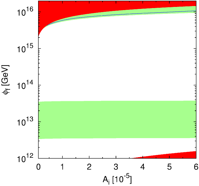
Figure 1: The two green/lightly shaded bands in the $A_{i}-\phi_{f}$ plane which lead to the PQ vacua at $t_{\phi}$ for $\kappa=3\times 10^{-3}$, $\lambda=10^{-4}$ (model A). The white (not shaded) areas lead to the trivial vacuum and are thus excluded. The upper red/dark shaded area is excluded by the requirement that, at $t_{*}$, $V^{\prime\prime}\leq H_{\rm infl}^{2}$, while the lower one corresponds to the quantum regime. The blue/solid line shows the values of $A_{i}$, $\phi_{f}$ which approximately reproduce the correct value of the CMBR large scale temperature anisotropy, as measured by COBE.

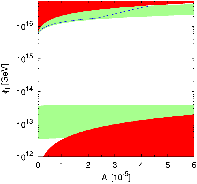
Figure 2: The two green/lightly shaded bands in the $A_{i}-\phi_{f}$ plane which lead to the PQ vacua at $t_{\phi}$ for $\kappa=3\times 10^{-2}$, $\lambda=10^{-4}$ (model B). The notation is the same as in Fig. 1.

We must first require that $N_{\rm max}\geq N_{Q}$. The time $t_{*}$ is then found from $N_{Q}=H_{\rm infl}(t_{f}-t_{*})$. Furthermore, we demand that, at $t_{*}$, $V^{\prime\prime}\leq H_{\rm infl}^{2}$, which ensures that this inequality holds for all times between $t_{*}$ and $t_{f}$. This guarantees that $\phi$ is effectively massless during inflation and can act as curvaton. It also justifies the use of the slow-roll approximation and ensures that the velocity of $\phi$ at the end of inflation is negligible. This masslessness requirement yields an upper bound on $\phi_{f}$ for every $A_{i}$ and fixed $\kappa$ and $\lambda$. The excluded region in the $A_{i}-\phi_{f}$ plane for fixed $\kappa$ and $\lambda$ is depicted as a red/dark shaded area in the upper part of this plane. In Figs. 1 and 2, we show this upper red/dark shaded area for $\kappa=3\times 10^{-3}$, $\lambda=10^{-4}$ (model A) and $\kappa=3\times 10^{-2}$, $\lambda=10^{-4}$ (model B) respectively. The lower red/dark shaded area corresponds to the quantum regime and is also excluded.

We start from any given $\phi_{f}$ at $t_{f}$ not excluded by the above considerations and assume zero time derivative of $\phi$ at $t_{f}$. We then follow the evolution of $\phi$ for $t\geq t_{f}$ by solving the equation of motion in Eq. (10) with $H=2/3t$ for $t_{f}\leq t\leq t_{\rm reh}$ and $H=1/2(t-t_{\rm reh}/4)$ for $t_{\rm reh}\leq t\leq t_{\phi}$. The time of reheating $t_{\rm reh}$ is found from Eq. (8) with $g_{*}=228.75$ and the curvaton decay time $t_{\phi}$ from Eq. (13) with $\beta$ from Eq. (6), where we put $\mu=300~{}{\rm GeV}$. We take $\gamma=0.1$ after the end of inflation. We find that, for fixed $\kappa$ and $\lambda$, there exist two bands in the $A_{i}-\phi_{f}$ plane leading to the PQ vacua at $t_{\phi}$. They are depicted as an upper and a lower green/lightly shaded band (see Figs. 1 and 2). The white (not shaded) areas in the $A_{i}-\phi_{f}$ plane lead to the false (trivial) minimum at $\phi=0$ and thus must be excluded.

7.2 The calculation of $C_{\ell}$

For any fixed $\kappa$ and $\lambda$, we take a grid of values of $A_{i}$ and $\phi_{f}$ which span the corresponding upper or lower green/lightly shaded band. For each point on this grid, we consider $\phi_{f}$ and its perturbed value $\phi_{f}+\delta\phi_{f}$ and follow the evolution of both these fields until curvaton decay (at $t_{\phi}$), where we evaluate the amplitude of $\delta\rho_{\phi}/\rho_{\phi}$. The amplitude $A_{c}$ is then given by Eq. (32). For the Monte Carlo (MC) analysis, we use $A_{i}$ and $A_{c}$ (rather than $A_{i}$ and $\phi_{f}$) as base parameters and limit our grid to $A_{i}\leq 6\times 10^{-5}$. The indices $n_{i}$ and $n_{c}$ for each point on the grid are found from Eqs. (21) and (22) applied at $x=x_{Q}$, and Eqs. (24), (30) and (33) applied at $t_{*}$. The fraction $f$ in Eq. (16) is evaluated at $t_{\phi}$. The amplitude $A_{a}$ of the isocurvature perturbation in the axions is calculated from Eq. (38) with the initial misalignment angle $\theta$ evaluated, for any given total CDM abundance $\Omega_{\rm CDM}h^{2}=\Omega_{\rm LSP}h^{2}+\Omega_{a}h^{2}$, by using Eqs. (39) and (40) with $m_{\rm LSP}=200~{}{\rm GeV}$. For our choice of parameters, the LSP relic abundance is fixed ($\simeq 0.0074$). The spectral index for axions is found from Eq. (41).

In summary, for any fixed $\kappa$ and $\lambda$, we take a grid in the variables $A_{i}$ and $A_{c}$ covering the upper or lower green/lightly shaded band. For any $\Omega_{B}h^{2}$ and $\Omega_{a}h^{2}$, we then calculate the amplitudes squared of the adiabatic and isocurvature perturbations from Eqs. (44), (45) and Eqs. (47), (48) respectively, the cross correlation amplitude from Eqs. (49), (50) and the total CMBR TT and TE power spectra via Eqs. (52)$-$(55). The curvaton fractional contribution to the adiabatic amplitude $F^{\rm ad}_{c}$, the dimensionless cross correlation $\cos\Delta$ and the entropy-to-adiabatic ratio $B$ are found from Eqs. (46) and (51). In computing $M$, $A_{c}$ and $A_{a}$, we fix the present Hubble parameter to the Hubble space telescope (HST) central value $H_{0}=72~{}\rm{km}~{}\rm{sec}^{-1}~{}\rm{Mpc}^{-1}$ [35], which has an impact less than 3% on our results. Clearly, we do allow $H_{0}$ to vary in the MC analysis.

Before deploying the full MC machinery to derive constraints on the parameters, it is instructive to obtain a first rough idea about the viability of our model by using the approximate expressions in Eqs. (57) and (58) for the temperature SW plateau and requiring that the COBE constraint in Eq. (56) is fulfilled. To this end, we take $\Omega_{B}h^{2}=0.0224$ and $\Omega_{\rm CDM}h^{2}=0.1126$, which are the best-fit values from WMAP [7]. We find that the COBE constraint cannot be satisfied in the lower green/lightly shaded band in the $A_{i}-\phi_{f}$ plane for any $\kappa$ and $\lambda$. The reason is that the relatively low values of $\phi_{*}$ in this band combined with the sizable relic abundance of the axions leads to an unacceptably large axion contribution to the RHS of Eq. (57). In the upper green/lightly shaded band in the $A_{i}-\phi_{f}$ plane, on the contrary, the COBE constraint is easily satisfied. The resulting solution is depicted by a blue/solid line (see Figs. 1 and 2).

7.3 The MC analysis

We proceed to the full MC analysis confronting the predictions of our model with the CMBR data. We use a version of the Markov chain MC package cosmomc [36] as described in Ref. [37]. The adiabatic and isocurvature CMBR transfer functions are computed in two successive calls similarly to Ref. [38]. For fixed $\kappa$ and $\lambda$, the initial conditions are fully specified by $A_{i}$ and $A_{c}$. The MC sampling takes as free parameters the $A_{i}$ and $A_{c}$, the present baryon and axion abundances $\omega_{B}\equiv\Omega_{B}h^{2}$ and $\omega_{a}\equiv\Omega_{a}h^{2}$, the present dimensionless Hubble parameter $h$, and the redshift $z_{r}$ at which the reionization fraction is a half. All other derived quantities are computed from the above parameter set. In particular, the total CDM abundance is $\omega_{\rm CDM}\equiv\Omega_{\rm CDM}h^{2}=\omega_{\rm LSP}+\omega_{a}$, where $\omega_{\rm LSP}\equiv\Omega_{\rm LSP}h^{2}\approx 0.0074={\rm constant}$. Also, since we take flat cosmologies only, the cosmological constant energy density $\Omega_{\Lambda}$ (in units of $\rho_{c}$) is a derived parameter, i.e. $\Omega_{\Lambda}=1-(\omega_{\rm CDM}+\omega_{B})/h^{2}$. The gravitational waves are negligible. In summary, for fixed $\kappa$ and $\lambda$, our parameter space is six dimensional:

$$\{\omega_{B},\omega_{a},h,z_{r},A_{i},A_{c}\}.$$ (60)

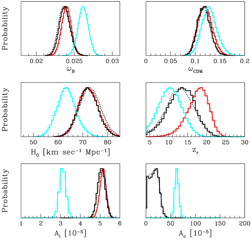
Figure 3: 1D marginalized posterior distribution for model A (black solid line) and model B (cyan/light gray solid line) with only the upper green/lightly shaded bands included. The red/medium gray line is for the pure inflaton case with $n_{i}=1$, plotted here for comparison. Model A is quite close to the pure inflaton case. Model B displays a preference for non-zero curvaton contribution. Its quality of fit is, however, poorer. We also display as dotted smoothed curves the values of the mean posterior. All the curves are normalized at their peak value.

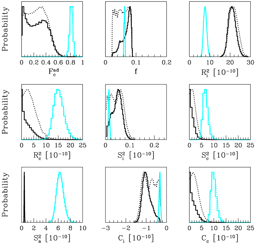
Figure 4: As in Fig. 3, but for (most of) the derived parameters (the pure inflaton model is not included). The adiabatic amplitude in model B is dominated by the curvaton ($F_{c}^{\rm ad}\approx 0.8$).

We compare the predicted CMBR TT and TE power spectra to the WMAP first-year data [7] with the routine for computing the likelihood supplied by the WMAP team [39]. At a smaller angular scale, we add the cosmic background imager (CBI) [40] and the decorrelated arcminute cosmology bolometer array receiver (ACBAR) [41] band powers as well. We use flat top-hat priors on the base parameters

$$\omega_{B},\omega_{a},z_{r},A_{i},A_{c}.$$ (61)

The limits of the top-hat priors do not matter for parameter estimation, as long as the posterior density is negligible near the limits. However, the prior range of the accessible parameter space plays an important role in computing the Bayes factor for model testing. We limit the maximum range of $h$ by imposing a top-hat prior $0.40<h<1.00$ and we use the HST result [35]

$$L^{\rm HST}\propto\exp\left(\frac{h-h_{0}}{2\sigma}\right)^{2},$$ (62)

where $h_{0}=0.72$ and $\sigma=0.08$, by multiplying the likelihood function for the CMBR data by the above Gaussian likelihood. By trying different priors, we find [11] that the broad lines of the constraints for the PQ model are robust with respect to the choice of non-informative priors.

We will examine in some detail the models A and B, which are representative cases of the two possible behavior patterns of our PQ model. We first consider the upper green/lightly shaded band of these models. The 1-dimensional (1D) marginalized posterior distributions for the base and most of the derived parameters are plotted, respectively, in Figs. 3 and 4.

In the upper band of model A, the power spectra are dominated by the adiabatic inflaton contribution. The quality of the fit, as expressed by the maximum likelihood, is slightly better than for the pure inflaton case with $n_{i}=1$, which is not surprising since the curvaton contribution plays a modest role. The CMBR data yield the bound $A_{c}<43.2\times 10^{-5}$ at $95\%$ confidence level. The total TT power on large scales is slightly larger than the pure adiabatic part, which increases the height of the SW plateau relative to the height of the first adiabatic peak. This mimics the impact of a larger $z_{r}$, and explains why model A prefers a later reionization than the pure inflaton case.

The upper band of model B exhibits a preference for a non-vanishing curvaton amplitude with very high significance ($A_{c}=62.8\pm 10.4$). The overall quality of the fit is though worse than for model A (upper band) because this model does not reproduce with enough precision the shape of the first acoustic peak. Furthermore, this model shows a preference for a rather high baryon abundance ($\omega_{B}\approx 0.026$), which is in strong tension with the value indicated by BBN together with observations of the light elements abundance, which typically yields $\omega_{B}\approx 0.020\pm 0.002$ [42].

For the lower band of model A, the quality of the best fit is poor, whereas the lower band of model B is incapable of producing a spectrum in reasonable agreement with the data. Thus, the lower bands of these models are excluded.

So far we have derived parameter constraints for models A and B from the data. The next question is to compare the upper bands of these two models with the pure inflaton scale-invariant model and decide which of these three models is most favored by data. Model comparison is a different issue than parameter extraction and it can very well be that it arrives at a different conclusion. Indeed, it can be that the estimated value of a parameter under a model $\mathcal{M}_{1}$ is far from the null value predicted by model $\mathcal{M}_{2}$, but $\mathcal{M}_{1}$ is disfavored against $\mathcal{M}_{2}$ by Bayesian model testing. This is the case for $A_{c}$ in model B (upper band) compared to the pure inflaton model.

To apply Bayesian model testing, we compute the Bayes factor $B$ for models A and B (upper bands) comparing each of them to the pure inflaton model with $n_{i}=1$. We find [11] that $\ln B=-3.9$ and $-17.1$ in the two cases respectively. Thus, model A (upper band) is disfavored against the pure inflaton model with odds of $50$ to $1$, while model B (upper band) with odds of $10^{7}$ to $1$. So, model B (upper band), which predicts a non-zero curvaton contribution to the adiabatic perturbation, is strongly disfavored. On the contrary, model A (upper band), which does not require such a contribution, is only mildly disfavored. However, in view of the fact that it addresses many issues lying outside the scope of the pure inflaton model, such as the strong CP and $\mu$ problems, the generation of the BAU and the nature of CDM, we can by no means reject it.

8 CONCLUSIONS

We studied a SUSY GUT model solving the strong CP and $\mu$ problems via a PQ symmetry and leading to standard hybrid inflation. The PQ field acts as curvaton contributing to the curvature perturbation together with the inflaton. The model predicts isocurvature perturbation too of mixed correlation with the adiabatic one. We confronted the predictions of the model with the CMBR data from WMAP, CBI and ACBAR and found that a non-zero curvaton contribution to the adiabatic perturbation is not favored.

References

- [1] A.R. Liddle and D.H. Lyth, Cosmological inflation and large-scale structure, Cambridge Univ. Press, Cambridge, 2000.
- [2] G. Lazarides, Lect. Notes Phys. 592 (2002) 351 [hep-ph/0111328]; hep-ph/0204294.
- [3] S. Mollerach, Phys. Rev. D 42 (1990) 313; A.D. Linde and V. Mukhanov, ibid. 56 (1997) 535.
- [4] D.H. Lyth and D. Wands, Phys. Lett. B 524 (2002) 5; T. Moroi and T. Takahashi, ibid. 522 (2001) 215; 539 (2002) 303(E).
- [5] D.H. Lyth, C. Ungarelli and D. Wands, Phys. Rev. D 67 (2003) 023503.
- [6] K. Dimopoulos and D.H. Lyth, Phys. Rev. D 69 (2004) 123509.
- [7] C.L. Bennett et al., Astrophys. J. Suppl. 148 (2003) 1; G. Hinshaw et al., ibid. 148 (2003) 135; A. Kogut et al., ibid. 148 (2003) 161; D.N. Spergel et al., ibid. 148 (2003) 175.
- [8] H.V. Peiris et al., Astrophys. J. Suppl. 148 (2003) 213.
- [9] C. Gordon and A. Lewis, Phys. Rev. D 67 (2003) 123513; P. Crotty, J. García-Bellido, J. Lesgourgues and A. Riazuelo, Phys. Rev. Lett. 91 (2003) 171301; M. Bucher, J. Dunkley, P.G. Ferreira, K. Moodley and C. Skordis, ibid. 93 (2004) 081301; K. Moodley, M. Bucher, J. Dunkley, P.G. Ferreira and C. Skordis, Phys. Rev. D 70 (2004) 103520.
- [10] C. Gordon and K.A. Malik, Phys. Rev. D 69 (2004) 063508; M. Beltrán, J. García-Bellido, J. Lesgourgues and A. Riazuelo, ibid. 70 (2004) 103530.
- [11] G. Lazarides, R. Ruiz de Austri and R. Trotta, Phys. Rev. D 70 (2004) 123527.
- [12] G. Lazarides and N.D. Vlachos, Phys. Lett. B 459 (1999) 482; G. lazarides, hep-ph/9905450.
- [13] E.J. Copeland, A.R. Liddle, D.H. Lyth, E.D. Stewart and D. Wands, Phys. Rev. D 49 (1994) 6410.
- [14] G. Dvali, Q. Shafi and R. Schaefer, Phys. Rev. Lett. 73 (1994) 1886.
- [15] K. Dimopoulos, G. Lazarides, D. Lyth and R. Ruiz de Austri, J. High Energy Phys. 05 (2003) 057.
- [16] G. Lazarides and Q. Shafi, Phys. Rev. D 58 (1998) 071702.
- [17] A.D. Linde, Phys. Lett. B 259 (1991) 38; Phys. Rev. D 49 (1994) 748.
- [18] J.E. Kim and H.P. Nilles, Phys. Lett. B 138 (1984) 150.
- [19] M. Dine, W. Fischler and D. Nemeschansky, Phys. Lett. B 136 (1984) 169; G.D. Coughlan, R. Holman, P. Ramond and G.G. Ross, ibid. 140 (1984) 44.
- [20] M. Dine, L. Randall and S. Thomas, Phys. Rev. Lett. 75 (1995) 398; Nucl. Phys. B 458 (1996) 291.
- [21] E.D. Stewart, Phys. Rev. D 51 (1995) 6847; M.K. Gaillard, H. Murayama and K.A. Olive, Phys. Lett. B 355 (1995) 71; M.K. Gaillard, D.H. Lyth and H. Murayama, Phys. Rev. D 58 (1998) 123505; C. Panagiotakopoulos, Phys. Lett. B 459 (1999) 473; R. Jeannerot, S. Khalil and G. Lazarides, J. High Energy Phys. 07 (2002) 069.
- [22] J.R. Ellis, J.E. Kim and D.V. Nanopoulos, Phys. Lett. B 145 (1984) 181; J.R. Ellis, D.V. Nanopoulos and S. Sarkar, Nucl. Phys. B 259 (1985) 175; J.R. Ellis, G.B. Gelmini, J.L. Lopez, D.V. Nanopoulos and S. Sarkar, ibid. 373 (1992) 399.
- [23] R.J. Scherrer and M.S. Turner, Phys. Rev. D 31 (1985) 681 .
- [24] K. Dimopoulos and D.H. Lyth, private communication.
- [25] K. Dimopoulos, D.H. Lyth, A. Notari and A. Riotto, J. High Energy Phys. 07 (2003) 053.
- [26] R. Allahverdi, B.A. Campbell and J.R. Ellis, Nucl. Phys. B 579 (2000) 355; A. Anisimov and M. Dine, ibid. 619 (2001) 729.
- [27] M. Fukugita and T. Yanagida, Phys. Lett. B 174 (1986) 45.
- [28] G. Lazarides and Q. Shafi, Phys. Lett. B 258 (1991) 305; G. Lazarides, R.K. Schaefer and Q. Shafi, Phys. Rev. D 56 (1997) 1324.
- [29] M. Kawasaki and T. Moroi, Prog. Theor. Phys. 93 (1995) 879.
- [30] M.S. Turner, Phys. Rev. D 33 (1986) 889.
- [31] E.J. Copeland, I.J. Grivell and A.R. Liddle, astro-ph/ 9712028.
- [32] L. Amendola, C. Gordon, D. Wands and M. Sasaki, Phys. Rev. Lett. 88 (2002) 211302.
- [33] R. Trotta, astro-ph/0410115.
- [34] M. Tegmark and A.J.S. Hamilton, astro-ph/9702019.
- [35] W.L. Freedman et al., Astrophys. J. 553 (2001) 47.
- [36] http://cosmologist.info/cosmomc/.
- [37] A. Lewis and S. Bridle, Phys. Rev. D 66 (2002) 103511.
- [38] J. Väliviita and V. Muhonen, Phys. Rev. Lett. 91 (2003) 131302.
- [39] L. Verde et al., Astrophys. J. Suppl. 148 (2003) 195.
- [40] T.J. Pearson et al., Astrophys. J. 591 (2003) 556.
- [41] J.H. Goldstein et al., Astrophys. J. 599 (2003) 773; C.-l. Kuo et al., ibid. 600 (2004) 32; http://cosmologist.info/ACBAR.
- [42] S. Burles, K.M. Nollett and M.S. Turner, Phys. Rev. D 63 (2001) 063512.