Quark-model study of few-baryon systems

Abstract

We review the application of non-relativistic constituent quark models to study one, two and three non-strange baryon systems. We present results for the baryon spectra, potentials and observables of the NN, N$\Delta$, $\Delta\Delta$ and NN${}^{*}(1440)$ systems, and also for the binding energies of three non-strange baryon systems. We make emphasis on observable effects related to quark antisymmetry and its interplay with quark dynamics.

1 Introduction

Hadron physics, ranging from particle to nuclear physics, aims to a precise and consistent description of hadronic structure and interactions. This is a formidable task that can only be ideally accomplished within the framework of the Standard Model of the strong and electroweak interactions. The strong interaction part, Quantum Chromodynamics (QCD), should give account of the main bulk of hadronic data but in its current state of development this objective seems far from being attainable. This has motivated the formulation of alternative descriptions, based on QCD and/or phenomenology, which restrict their study to a particular set of hadronic systems and are able to reproduce the data and to make useful testable predictions. In this sense non-relativistic constituent quark models incorporating chiral potentials provide undoubtedly the most successful, consistent and universal microscopic description of the baryon spectrum and the baryon-baryon interaction altogether. Therefore they are ideal frameworks to analyze few-baryon systems. The purpose of this review article is to report the progress made in the last years in this analysis. But first to put these models in perspective we shall start by recalling the main aspects of the different approaches in hadron physics. Then we shall present the historical development of chiral constituent quark models emphasizing their connection to phenomenology and their plausible relation to the basic theory.

QCD [1] is nowadays accepted as the basic theory to describe the hadrons and their strong interactions. QCD is a renormalizable quantum field theory of quarks and gluons based on a local gauge principle on the group $SU(3)_{Colour}$. Apart from this local symmetry the QCD Lagrangian has also, for massless quarks, a global $SU(n)\times SU(n)$ ($n$: number of quark flavours) chiral symmetry that appears to be spontaneously broken in nature. Other relevant properties of QCD are related to the running of the quark-gluon coupling constant: for high momenta (i.e., high momentum transfers as compared to the QCD scale, $\Lambda_{\rm QCD}$) the coupling tends to vanish and the quarks are essentially free, a property named asymptotic freedom; for low momenta the coupling becomes strong, a property known as infrared slavery. As a consequence of this behaviour a solution of the theory is only attainable, perturbatively, at high momenta. In the low-momentum regime one has to resort to non-perturbative calculation methods (sum rules, instanton based calculations,…) of limited applicability or to reformulations of the theory from which to approach the exact solution. Thus lattice QCD has been developed in the hope of getting from it the exact solution by a limiting procedure from the discrete lattice space to the continuum. However progress in making precise, detailed predictions of the physical states of the theory is slow (due in part to the enormous computer capacity required) [2].

Alternatively effective field theory approaches have been proposed: from the action and measure of QCD one can integrate out the irrelevant degrees of freedom in the momentum region under consideration to obtain a more tractable field theory with the same $S$ matrix. This procedure, used with notable precision at high momenta where the smallness of the coupling constant makes feasible to calculate the effective Lagrangian, cannot be pursued with the same precision at low momenta. Such a difficulty can be overcome by the application of a celebrated, though unproven, theorem by Weinberg [3] which states that one should write the most general Lagrangian, constructed from the accessible degrees of freedom in the momentum region under consideration, which satisfies the relevant symmetries of the theory. This is the scheme used in Chiral Perturbation Theory [4] which has been successful in the study of low momentum hadron (in particular meson) physics.

Other approaches take limits of QCD and generate from them systematic expansions to get corrections. Among them we shall briefly comment on the Heavy Quark Effective Theory (HQET) [5], the Non-Relativistic QCD (NRQCD) [6] and the $1/N_{c}$ approach [7, 8].

For physical systems with a heavy quark, interacting with light quarks and gluons carrying a momentum of order $\Lambda_{\rm QCD}$, an appropriate limit of QCD involves taking the heavy quark mass going to infinity, $m_{Q}\rightarrow\infty$ (HQET). In this limit the strong interactions of the heavy quark become independent of its mass and spin. These heavy flavour and spin symmetries, not present in QCD, lead to model independent relations that allow for instance the description of exclusive decays in terms of a few parameters. Corrections are obtained from an expansion in terms of $1/m_{Q}$, the inverse of the heavy quark mass.

When more than one heavy quark is present in the system (for example in quarkonia) the heavy quark kinetic energy, treated as a small correction in HQET, cannot be treated as a perturbation. For such systems the appropriate limit of QCD to examine is the $c\rightarrow\infty$ limit (or $v/c\rightarrow 0$ in quarkonia, being $v$ the relative heavy quark velocity and $c$ the speed of light). The resulting field theory is called Non-Relativistic QCD. An expansion in terms of $1/c$ is done. NRQCD has improved the understanding of the decays and production of quarkonia.

The $1/N_{c}$ approach is the limit of QCD when the number of colours $N_{c}$ tends to infinity. An expansion in terms of $1/N_{c}$, the inverse of the number of colours, is performed. Remarkably, large $N_{c}$ QCD reduces smoothly to an effective field theory of non-interacting mesons to leading order. Baryons emerge as solitons in this weakly coupled phase of mesons. This is the base of topological models where baryons are constructed from non-linear meson fields in chiral Lagrangians (Skyrme model [9], chiral soliton model [10],…)

At a much more phenomenological level model building has been extremely useful to provide a classification of hadronic data and to make predictions. Though the connection with QCD is not clearly established and there is not a sound systematics to obtain corrections, models provide simple physical pictures which connect the phenomenological regularities observed in the hadron data with the underlying structure.

Historically the first model of hadron structure, a non-relativistic quark model, appeared in the nineteen sixties right after Gell-Mann and Zweig [11, 12] introduced the quarks as the members of the triplet representation of $SU(3)_{Flavour}$ from which the hadron representations could be constructed. The lack of observation of free quarks in nature seemed to indicate their strong binding inside hadrons. Dalitz [13] performed a quark model analysis of hadronic data based on flavour. This analysis seemed to point out some possible inconsistencies with the Spin-Statistic theorem. The introduction of colour [14, 15], a new degree of freedom for the quarks, saved the consistency and led to the formulation of QCD. The other way around QCD provided from its infrared slavery property some justification for coloured quark confinement inside colour singlet hadrons. Moreover an interquark colour potential was derived by de Rújula, Georgi and Glashow [16] from the one-gluon exchange (OGE) diagram in QCD, and applied in an effective manner to reproduce energy splittings in hadron spectroscopy.

In the 70’s the potentialities of quark model calculations in hadronic physics were established. The non-relativistic quark model was formulated under the assumption that the hadrons are colour singlet non relativistic bound states of constituent quarks with phenomenological effective masses and interactions.

Non-relativistic quark models incorporating effective OGE and confinement potentials provided in the heavy meson sector a very good description of the charmonium and bottomonium spectra [17, 18]. The reasonable results obtained when applied to the light baryon sector [19] were somewhat surprising since according to the size of the baryons ($\sim$ 0.8 fm) and the mass of the light constituent quarks employed ($m_{u}=m_{d}\simeq$ 300 MeV) the quark velocities were close to $c$ and the non-relativistic treatment could hardly be justified. In the spirit of quark potential model calculations this pointed out that the effectiveness of the parameters of the potential could be taking, at least partially into account in an implicit form, some relativistic corrections. Years later the low-lying states of the meson [20] and baryon spectra [21] were reasonably reproduced with a unique set of parameter values.

On the same line relativistic quark models started to be developed. The bag model [22] considered asymptotically free quarks confined into a space-time tube through field boundary conditions. Chiral symmetry was incorporated through current conservation at the boundary associated to the presence of a meson cloud [23]. Hadron spectra and properties were calculated. However, despite the very intuitive image the bag model provided of a nucleon as a quark core surrounded by a meson cloud, calculations had to face the technical difficulty of separating the center of mass motion, an endemic problem in all relativistic quark models.

Mid-way between non-relativistic and relativistic treatments semirelativistic quark models, where the relativistic expression for the kinetic energy was used in the Schrödinger equation, were explored [24].

At the same time there were attempts to study the hadron-hadron interaction within the non-relativistic quark model framework [25]. It was soon realized that the colour structure of the OGE interquark potential could provide an explanation for the nucleon-nucleon (NN) short-range repulsion [26]. This encouraged several groups to undertake the ambitious project of describing the NN interaction from the quark-quark (confinement+OGE) potential [27, 28, 29, 30, 32, 33, 31] by using the resonating group method or Born-Oppenheimer techniques. According to the expectations a quantitative explanation for the short-range NN repulsion was found. However, for the medium and long-range parts of the NN interaction, though $(q\overline{q})$ and $(q\overline{q})^{2}$ excitations generated by off-shell terms of the Fermi-Breit piece of the OGE were considered so that the NN potential became attractive in the $0.8-1.5$ fm range, the attraction was too weak to bind the deuteron or to fit the extreme low-energy $S$-wave scattering [34].

To remedy this hybrid quark models [35, 36] containing both, interquark (confinement+OGE) and interbaryon long-range one-pion and medium range one-sigma, or two-pion exchange potentials, were introduced. Although these models were efficient to reproduce scattering and bound state data it was compelling, for the sake of consistency, to find a justification for these interbaryon potentials at the quark level. By considering that they could be due to (chiral) meson clouds surrounding the nucleons quark core, and pursuing the philosophy initiated in [16] of trying to incorporate into the quark potential model the dynamics and symmetries of QCD, an implementation of chiral symmetry at the quark potential level was needed.

To accomplish this task the progress in the understanding of the connection between quark potential models and the basic theory was of great help. Manohar and Georgi [37] argued that the scale associated to confinement in a hadron ($\Lambda_{\rm CON}\sim$ 100$-$300 MeV) being smaller than the one associated to chiral symmetry breaking $(\Lambda\sim$ 1 GeV) would drive to a picture where quarks, gluons and pions coexisted in a region of momentum. Using an effective field theory approach they obtained a model where constituent quarks (with a mass generated through chiral symmetry breaking) and gluons interacted via conventional colour couplings while quarks and pions did via a non-linear sigma model. By the same time Diakonov, Petrov and Yu got similar results concerning chiral symmetry breaking from a picture of the QCD vacuum as a dilute gas of instantons [38, 39].

The effect of incorporating to the simple (confinement+OGE) model a one-pion exchange (OPE) potential at the quark level started to be analyzed. It was realized that the OPE potential gave rise to a NN short-range repulsion [40] to be added to the OGE one. As a consequence the quark-gluon coupling constant needed to fit the data got nicely reduced from its former effective value ($>$1) to a value ($<$1) much more according to the perturbative derivation of the OGE from QCD. The same conclusion came out from the OPE contribution to the $\Delta-$N mass difference [41]. On the other hand the OPE potential generated, at large internucleonic distances, a NN conventional pion exchange interaction as needed. Nonetheless at the medium range it did not provide enough NN attraction to fit the data.

The introduction of sigma as well as pion exchanges between the quarks, in the form dictated by a Nambu-Goldstone realization of chiral symmetry within the linear sigma model, allowed to overcome this problem. Thus, the first non-relativistic constituent quark model of the NN interaction incorporating a chiral $SU(2)\times SU(2)$ potential came out [42, 43]. NN phase shifts (with the exception of $P$-waves) and deuteron properties were satisfactorily described. Furthermore, reasonable, though not precise, hadron spectra were predicted with the very same model (i.e. with the same set of parameters fitted from the NN interaction) [42, 44]. This model has been usually referred in the literature as chiral constituent quark model (CCQM). We shall maintain this logo hereforth.

Later on a $SU(3)\times SU(3)$ chiral quark model where constituent quarks interact only through pseudoscalar Goldstone bosons (GBE) was developed to describe very successfully the baryon spectra [45]. However its application to the NN interaction revealed a too strong tensor force, generated from the $\pi$-exchange, and the absence of the necessary medium-range attraction [46]. When properly implemented with the one-gluon exchange and scalar $SU(3)\times SU(3)$ Goldstone boson interactions, these models were successfully applied to the NN and nucleon-hyperon interactions [47, 48].

The significant role played by the semirelativistic kinematics in the GBE model to fit the spectroscopy encouraged the implementation of a relativistic treatment in the CCQM. When done [49] a pretty nice description of the non-strange baryon spectra was obtained as well.

The success in the description of the non-strange baryon spectroscopy and the NN interaction in a consistent manner makes the CCQM to be a powerful tool to treat, in a parameter-free way and on the same footing, other baryon-baryon interactions. This consistent treatment is mandatory in the study of few-baryon systems due to the intertwined role of nucleons and resonances in them. In this article we review the application of non-relativistic constituent quark models to obtain the energy spectra of hadrons and the baryon-baryon effective potentials (we will not consider baryon form-factors or amplitudes for weak, electromagnetic or strong decays since they are very sensitive to relativity [50]). Though most of the results will refer to the CCQM, results from other models will be included for completeness. The order of the presentation is the following. In section 2 the derivation of the chiral part of the quark-quark potential from an effective Lagrangian, incorporating spontaneous chiral symmetry breaking, is detailed. A one-gluon exchange potential, giving account of the residual (perturbative) colour interaction, completes the quark-quark potential whose parameters are fitted from the NN interaction and the non-strange baryon spectrum. In order to be able to generate a baryon-baryon potential from the quark-quark one and to deepen the understanding of the role played by quark antisymmetry, a variational two-baryon wave function is introduced in section 3. A detailed explanation of the NN short-range repulsion based on the interplay between quark antisymmetry and dynamics is presented. The baryon-baryon potential for NN, N$\Delta$, $\Delta\Delta$ and NN^∗(1440) channels are constructed in section 4 and section 5. Comparison to experimental data, when available, and to other model results, are shown. A coupled channel calculation for the NN system above the pion threshold is reported. In section 6 a thorough study of the non-strange baryon spectrum is carried out. Some related comments on the first experimental candidate for an exotic baryon, the $\Theta^{+}$ resonance, are also included. Consistency of the baryon spectrum wave functions with the variational baryon-baryon wave functions is shown. Section 7 is devoted to the search for unstable two- and three-baryon resonances. A more complete calculation for the triton binding energy is presented. Finally in section 8 we summarize the main results and conclusions.

2 The chiral constituent quark model.

2.1 The quark-quark potential

In non-relativistic quark models quark colour confinement inside colour singlet hadrons is taken for granted. Though confinement has not been rigorously derived from QCD, lattice calculations show in the so-called quenched approximation (only valence quarks) an interquark potential linearly increasing with the interquark distance [51]. This potential can be physically interpreted in a picture in which the quarks are linked with a one-dimensional colour flux tube or string and hence the potential is proportional to the distance between the quarks,

$$V_{\rm{CON}}({\vec{r}}_{ij})=-a_{c}\,{\vec{\lambda}}_{i}\cdot{\vec{\lambda}}_{j}\,r_{ij},$$ (2.1)

where $a_{c}$ is the confinement strength, the ${\vec{\lambda}}$’s are the $SU(3)$ colour matrices, and the colour structure prevents from having confining interaction between colour singlets [52]. Hadron sizes correspond to a scale of confinement $\Lambda_{\rm CON}\sim$ 100$-$300 MeV. On the other hand low-lying hadron masses are much bigger than light quark (up and down) current masses in QCD. So when dealing with hadrons one can reasonably assume as a good approximation the light quarks to be massless.

In the limit of zero light-quark masses the QCD Lagrangian is invariant under the chiral transformation $SU(2)_{L}\otimes SU(2)_{R}$. This symmetry would imply the existence of chiral partners, that is, for each low-lying hadron there would exist another one with equal mass and opposite parity . This is not observed in nature what points out to a spontaneous chiral symmetry breaking in QCD. As a consequence, the current quarks get dressed becoming constituent quarks and Goldstone bosons are generated [55]. Would the whole process be exact, one would end up with massless Goldstone bosons exchanged between the constituent quarks. In the real world chiral symmetry is only an approximate symmetry so one ends up with low-mass bosons (with masses related to the quark masses) exchanged between the constituents.

The picture of the QCD vacuum as a dilute medium of instantons [38, 39] explains nicely the spontaneous chiral symmetry breaking, which is the most important non-perturbative phenomenon for hadron structure at low momenta. Quarks interact with fermionic zero modes of the individual instantons in the medium and therefore the propagator of a light quark gets modified and quarks acquire a momentum dependent mass which drops to zero for momenta higher than the inverse of the average instanton size $\overline{\rho}$. The momentum dependent quark mass acts as a natural cutoff of the theory. In the domain of momenta $q<1/\overline{\rho}$, a simple chiral invariant Lagrangian can be derived as [38]

$$L=\overline{\psi}(\rmi\gamma^{\mu}\partial_{\mu}-MU^{\gamma_{5}})\psi$$ (2.2)

where $U^{\gamma_{5}}=\exp(i\vec{\pi}\cdot\vec{\tau}\gamma_{5}/f_{\pi})$. $\vec{\pi}$ denotes a Goldstone pseudoscalar field, $f_{\pi}$ is the pion decay constant, and $M$ is the constituent quark mass. The momentum dependence of the constituent quark mass can be obtained from the theory. It has been effectively parametrized as $M(q^{2})=m_{q}F(q^{2})$ [41, 43] with

$$F(q^{2})=\left[\frac{\Lambda^{2}}{\Lambda^{2}+q^{2}}\right]^{\frac{1}{2}}$$ (2.3)

where $\Lambda$ is the chiral symmetry breaking scale, $\Lambda\sim 1/\overline{\rho}$ and $m_{q}=M(q^{2}=0)\approx$ 350 MeV. We shall call hereforth $m_{q}$ the constituent quark mass. $U^{\gamma_{5}}$ can be expanded in terms of boson fields as,

$$U^{\gamma_{5}}=1+\frac{\rmi}{f_{\pi}}\gamma^{5}\vec{\tau}\cdot\vec{\pi}-\frac{1}{2f_{\pi}^{2}}\vec{\pi}\cdot\vec{\pi}+...$$ (2.4)

The first term generates the constituent quark mass and the second gives rise to a pseudoscalar (PS) one-boson exchange interaction between quarks. The main contribution of the third term comes from the two-pion exchange which is usually simulated by means of a scalar (S) exchange. From the non-relativistic approximation of the Lagrangian one can generate in the static approximation the quark-meson exchange potentials:

$$V_{\rm{PS}}({\vec{r}}_{ij})={1\over 3}\,\alpha_{\rm{ch}}{\Lambda^{2}\over\Lambda^{2}-m_{\rm{PS}}^{2}}\,m_{\rm{PS}}\,\Biggr{\{}\left[\,Y(m_{\rm{PS}}\,r_{ij})-{\Lambda^{3}\over m_{\rm{PS}}^{3}}\,Y(\Lambda\,r_{ij})\right]{\vec{\sigma}}_{i}\cdot{\vec{\sigma}}_{j}+$$

$$\left[H(m_{\rm{PS}}\,r_{ij})-{\Lambda^{3}\over m_{\rm{PS}}^{3}}\,H(\Lambda\,r_{ij})\right]S_{ij}\Biggr{\}}\,{\vec{\tau}}_{i}\cdot{\vec{\tau}}_{j}\,,$$ (2.5)

$$V_{\rm{S}}({\vec{r}}_{ij})=-\alpha_{\rm{ch}}\,{4\,m_{q}^{2}\over m_{\rm{PS}}^{2}}{\Lambda^{2}\over\Lambda^{2}-m_{\rm{S}}^{2}}\,m_{\rm{S}}\,\left[Y(m_{\rm{S}}\,r_{ij})-{\Lambda\over{m_{\rm{S}}}}\,Y(\Lambda\,r_{ij})\right]\,,$$ (2.6)

where the $i$ and $j$ indices are associated with $i$ and $j$ quarks respectively, ${\vec{r}}_{ij}$ stands for the interquark distance, $\alpha_{\rm{ch}}$ is the chiral coupling constant, the ${\vec{\sigma}}$’s (${\vec{\tau}}$’s) are the spin (isospin) quark Pauli matrices. $m_{\rm PS}$ and $m_{\rm S}$ are the masses of the pseudoscalar and scalar Goldstone bosons, respectively. $S_{ij}\,=\,3\,({\vec{\sigma}}_{i}\cdot{\hat{r}}_{ij})({\vec{\sigma}}_{j}\cdot{\hat{r}}_{ij})\,-\,{\vec{\sigma}}_{i}\cdot{\vec{\sigma}}_{j}$ is the quark tensor operator and $Y(x)$ and $H(x)$ are the standard Yukawa functions defined by $Y(x)=\rme^{-x}/x$ and $H(x)=(1+3/x+3/x^{2})Y(x)$.

For $q^{2}\gg\Lambda^{2}$ one expects QCD perturbative effects playing a role. They mimic the gluon fluctuations around the instanton vacuum and are taken into account through the OGE potential [16]. From the non-relativistic reduction of the one-gluon-exchange diagram in QCD for point-like quarks one gets

$$V_{\rm{OGE}}({\vec{r}}_{ij})={1\over 4}\,\alpha_{s}\,{\vec{\lambda}}_{i}\cdot{\vec{\lambda}}_{j}\Biggl{\{}{1\over r_{ij}}-{1\over{4\,m^{2}_{q}}}\,\biggl{[}1+{2\over 3}{\vec{\sigma}}_{i}\cdot{\vec{\sigma}}_{j}\biggr{]}\,\,{{\rme^{-r_{ij}/r_{0}}}\over{r_{0}^{2}\,\,r_{ij}}}-{3\over{4m^{2}_{q}\,r^{3}_{ij}}}\,S_{ij}\Biggr{\}}\,,$$ (2.7)

where $\alpha_{s}$ is an effective strong coupling constant. Let us realize that the contact term involving a Dirac $\delta(\vec{r})$ that comes out in the deduction of the potential has been regularized in the form

$$\delta(\vec{r}\,)\,\rightarrow\,{1\over{4\pi r_{0}^{2}}}\,\,{{\rme^{-r/r_{0}}}\over r}\,,$$ (2.8)

where $r_{0}$ is a regularization parameter giving rise to the second term of (2.7). This avoids to get an unbound baryon spectrum when solving the Schrödinger equation [56].

Thus the quark-quark interaction has the form,

$$V_{qq}(\vec{r}_{ij})=V_{\rm{CON}}(\vec{r}_{ij})+V_{\rm{OGE}}(\vec{r}_{ij})+V_{\rm{PS}}(\vec{r}_{ij})+V_{\rm{S}}(\vec{r}_{ij})\,.$$ (2.9)

Such a model has an immediate physical interpretation. In the intermediate region, between the scale at which the chiral flavour symmetry is spontaneously broken, $\Lambda\sim$ 0.8 GeV, and the confinement scale, $\Lambda_{\rm CON}\sim$ 0.2 GeV, QCD is formulated in terms of an effective theory of constituent chiral quarks interacting through the Goldstone modes associated with the spontaneous breaking of chiral symmetry. For $q^{2}\gg\Lambda^{2}$ gluon exchange is also important.

It is worthwhile to note that vector meson-exchange potentials ($\rho$, $\omega$) are not considered. The problem of unifying the quark exchange and meson exchange in the nuclear force has been a matter of discussion [57]. It has been shown that the pseudoscalar ($\pi$) and scalar ($\sigma$) meson-exchange terms can be simply added to the quark-exchange terms without risk of double counting. However, the vector-meson exchanges ($\rho$, $\omega$), which play an important role in meson-exchange models at the baryon level need some care. In baryonic one-boson exchange models, the $\omega$-meson provides the short-range repulsion of the NN interaction. In chiral constituent quark models this task is taken over by the antisymmetrization effects on the pseudoscalar exchange combined with OGE. Besides, the $\rho$-meson reduces the strength of the tensor pseudoscalar interaction, the same effect that is obtained from the quark-exchange terms of the pseudoscalar potential as has been checked in charge-exchange reactions [58].

2.2 Model parameters

In the spirit of quark model calculations the parameters in the potentials have an effective character. A rough estimate of the values of the parameters can be made based on general arguments. It is well established that the NN interaction at long-range is governed by the one-pion exchange. Therefore, to reproduce accurately this piece of the NN interaction, one is forced to identify the mass of the pseudoscalar field with the physical pion mass. The mass of the scalar field, the one-sigma exchange (OSE), is obtained by the PCAC relation [59]

$$m_{\rm{PS}}^{2} = m_{\pi}^{2}$$ (2.10)

$$m_{\rm{S}}^{2} = m^{2}_{\rm{PS}}+4m^{2}_{q}\,.$$

As the pseudoscalar field is identified with the pion, the $\alpha_{\rm ch}$ coupling constant should reproduce the long-range OPE interaction. If two nucleons are separated enough, the central part of $V_{\rm PS}$, the pseudoscalar interaction between quarks, generates an interaction between nucleons of the form,

$$V_{\rm{PS}}(R)=\frac{1}{3}\,\alpha_{\rm{ch}}\,G\,\,{\Lambda^{2}\over{\Lambda^{2}-m_{\pi}^{2}}}\frac{\rme^{-m_{\pi}R}}{R}\left(\frac{5}{3}\right)^{2}(\vec{\sigma}_{N}\cdot\vec{\sigma}_{N})(\vec{\tau}_{N}\cdot\vec{\tau}_{N})$$ (2.11)

where $R$ is the interbaryon distance and $G$ depends on the nucleon wave function. Comparing with the standard one-pion-exchange internucleon potential,

$$V_{\rm{OPE}}(R)=\frac{1}{3}\,\frac{f_{\pi\rm{NN}}^{2}}{4\pi}\,{\Lambda^{2}\over{\Lambda^{2}-m_{\pi}^{2}}}\frac{\rme^{-m_{\pi}R}}{R}(\vec{\sigma}_{N}\cdot\vec{\sigma}_{N})(\vec{\tau}_{N}\cdot\vec{\tau}_{N})$$ (2.12)

where the same form factor has been used at the quark and baryon levels, and using a harmonic oscillator wave function for the nucleon in terms of quarks (see next section), one finally obtains [60],

$$\alpha_{\rm{ch}}=\left(\frac{3}{5}\right)^{2}\frac{f_{\pi\rm{NN}}^{2}}{4\pi}\,\,\rme^{-\frac{b^{2}m_{\pi}^{2}}{2}}\,=\,\left(3\over 5\right)^{2}{g_{\pi\rm{NN}}^{2}\over{4\pi}}{m_{\pi}^{2}\over{4m_{N}^{2}}}\,\rme^{-\frac{b^{2}m_{\pi}^{2}}{2}}\,.$$ (2.13)

This gives the chiral coupling constant $\alpha_{\rm ch}$ in terms of the $\pi$NN coupling constant, taken to be $f_{\pi\rm{NN}}^{2}/4\pi=0.078$ [61], and $b$. Usual values in the literature for $b$ range between 0.4 and 0.6 fm. The most stringent determination, $b=$ 0.518 fm, was done in reference [62] by means of a simultaneous study of $S$-wave NN phase shifts and deuteron properties (see section 5). As it will be discussed, this value turns out to be consistent with the solution of the baryon spectra as a three-body problem in terms of the interaction (2.9) [44]. The value of $\alpha_{\rm ch}$ is then $\alpha_{\rm ch}=$0.0269.

The tensor force is mainly due to the pion interaction. Therefore, the value of $\Lambda$ can be fixed examining a process dominated by the tensor term. Such a reaction could be the $pp\to n\Delta^{++}$ because, at high momenta, more than $90\,\%$ of the interaction corresponds to the tensor part. The calculation of reference [58] suggests for $\Lambda$ a value close to 4.2 fm ^-1.

The value of $\alpha_{s}$ is estimated from the $\Delta-$N mass difference. In the chiral constituent quark model there are contributions not only from spin-spin term of the OGE but also from the pseudoscalar interaction, the latter contributing approximately half of the total mass difference. The rest is attributed to the OGE, and the value of $\alpha_{s}$ is adjusted to reproduce the experimental $\Delta-$N mass difference. This gives $\alpha_{s}\sim 0.4-0.5$ for $r_{0}=0.25$ fm, a standard value of $r_{0}$ within the stability region for the $\Delta-$N mass difference (see section 6.2.4).

The constituent quark mass $m_{q}$ is an effective parameter whose value is conventionally chosen in the range of 300 MeV, using in general smaller values for the study of the NN interaction and bigger ones for one-baryon properties. From the proton and neutron magnetic moments in the impulse approximation one gets $m_{q}=350$ MeV. From NN scattering the quark mass value should be close to one third of the nucleon mass $m_{q}\sim 1/3m_{N}\sim 313$ MeV. In this way a correct relation between the momentum and kinetic energy is guaranteed [27].

Table 1: Quark model parameters.

$m_{q}$	$b$	$\alpha_{s}$	$a_{c}$	$\alpha_{\rm{ch}}$	$r_{0}$	$m_{\rm{S}}$	$m_{\rm{PS}}$	$\Lambda$
(MeV)	(fm)		(MeV fm-1)		(fm)	(fm-1)	(fm-1)	(fm-1)
313	0.518	0.485	67.0	0.0269	0.25	3.42	0.7	4.2

Finally, regarding $a_{c}$ we should first notice that the contribution of confinement to the force between two baryons is very small (zero for quadratic confining, see section 3.2). Hence its value is only constrained by the requirement of having a confining ($a_{c}>0$) and not a deconfining ($a_{c}<0$) interaction. This can be guaranteed through the nucleon mass stability condition $\left.\partial M_{N}(b)/\partial b\right|_{b=0.518}=0$. Concerning its specific value we can resort to the baryon spectrum which is strongly dependent on it (see section 6). We quote in table 1 the standard value derived from the baryon spectrum analysis. Some caution is necessary when comparing the strength of the confining potential to other values given in the literature. First, one should be aware of the specific form used for the confining interaction, if the colour Gell-Mann matrices are used or not (a factor $-8/3$ is in the way). Second, when scalar potentials between quarks are used, as it is the case of the chiral constituent quark model, smaller values of $a_{c}$ than in pure OGE models are obtained.

The standard values of the parameters used in the chiral constituent quark model is resumed in table 1.

3 The non-strange two-baryon system

3.1 The two-baryon wave function: quark Pauli blocking

The calculation of the interaction between two baryons requires the knowledge of the two-baryon wave function and therefore that of a single baryon in terms of quarks. Single baryon wave functions have been calculated using different methods available in the literature to solve the three-body problem (see section 6). Although the resulting wave functions have an involved structure, it has been shown that for the baryon-baryon interaction they can be very well approximated by harmonic oscillator eigenfunctions [44]. For the non-strange baryons we are going to consider: N, $\Delta$ and N^∗(1440), the total wave function of a single baryon can be explicitly written as the product of three wave function components: spatial, spin-isospin, and colour space respectively,

$$|\Phi_{B}\rangle=\phi(\vec{r}_{1},\vec{r}_{2},\vec{r}_{3};\vec{R})\otimes\chi_{ST}\otimes\xi_{C}\,,$$ (3.1)

where $\vec{r}_{i}$ is the position of quark $i$ and $\vec{R}$ denotes the center of mass coordinate of the baryon. The symmetrization postulate requires the wave function to be antisymmetric. Explicitly,

$$\Phi_{\rm N}({\vec{r}}_{1},{\vec{r}}_{2},{\vec{r}}_{3};\vec{R})=\prod_{n=1}^{3}\left({\frac{1}{\pi b^{2}}}\right)^{3/4}\rme^{-{\frac{(\vec{r}_{n}-\vec{R})^{2}}{2b^{2}}}}\otimes[3]_{S=1/2,T=1/2}\otimes[1^{3}]_{C}\,,$$ (3.2)

$$\Phi_{\Delta}({\vec{r}}_{1},{\vec{r}}_{2},{\vec{r}}_{3};\vec{R})=\prod_{n=1}^{3}\left({\frac{1}{\pi b^{2}}}\right)^{3/4}\rme^{-{\frac{(\vec{r}_{n}-\vec{R})^{2}}{2b^{2}}}}\otimes[3]_{S=3/2,T=3/2}\otimes[1^{3}]_{C}\,,$$ (3.3)

$$\Phi_{{\rm N}^{*}(1440)}({\vec{r}}_{1},{\vec{r}}_{2},{\vec{r}}_{3};\vec{R})=\left(\sqrt{2\over 3}\phi_{1}-\sqrt{1\over 3}\phi_{2}\right)\otimes[3]_{S=1/2,T=1/2}\otimes[1^{3}]_{C}\,,$$ (3.4)

where $[3]_{ST}$ stands for a completely symmetric $SU(4)$ spin-isospin wave function and $[1^{3}]_{C}$ for a completely antisymmetric $SU(3)$ colour wave function [63], and

$$\phi_{1}({\vec{r}}_{1},{\vec{r}}_{2},{\vec{r}}_{3};\vec{R})={\sqrt{2}\over 3}\left({\frac{1}{\pi b^{2}}}\right)^{9/4}\sum_{k=1}^{3}\left[{\frac{3}{2}}-{\frac{(\vec{r}_{k}-\vec{R})^{2}}{b^{2}}}\right]\prod_{i=1}^{3}\rme^{-{\frac{(\vec{r}_{i}-\vec{R})^{2}}{2b^{2}}}},$$ (3.5)

$$\phi_{2}({\vec{r}}_{1},{\vec{r}}_{2},{\vec{r}}_{3};\vec{R})=-{2\over 3}\left(1\over\pi^{9\over 4}b^{13\over 2}\right)\sum_{j<k=1}^{3}(\vec{r}_{j}-\vec{R})\cdot(\vec{r}_{k}-\vec{R})\prod_{i=1}^{3}\rme^{-{\frac{(\vec{r}_{i}-\vec{R})^{2}}{2b^{2}}}}.$$ (3.6)

Once single baryon wave functions have been constructed, one can proceed to study the two-baryon wave functions. Again the symmetrization postulate forces the wave function of a system of $n$ identical quarks to be totally antisymmetric under the exchange of any two of them. As single baryon wave functions are already antisymmetric, there is an important simplification to construct two-baryon wave functions: one needs the antisymmetrizer for a system of six identical particles but already clustered in two antisymmetric groups. The antisymmetrizer can then be written as [64]

$${\cal A}={1\over N}\left(1-\sum_{i=1}^{3}\sum_{j=4}^{6}P_{ij}\right)(1-{\cal P})\,,$$ (3.7)

where $P_{ij}$ is the operator that exchanges particles $i$ and $j$, ${\cal P}$ exchanges the two clusters, and $N$ is a normalization constant. $P_{ij}$ can be explicitly written as the product of permutation operators in colour ($C$), spin-isospin ($ST$) and spatial ($O$) spaces,

$$P_{ij}=P^{C}_{ij}\;P^{ST}_{ij}\;P^{O}_{ij}\,.$$ (3.8)

Taking into account that any two-baryon state can be decomposed in a symmetric plus an antisymmetric part under the exchange of the baryon quantum numbers, one can write for a definite symmetry (specified by $f$ even or odd) and projecting onto a partial wave to make clear the effect of the exchange operator [65, 66]:

$$\Psi_{B_{1}B_{2}}^{LST}({\vec{R}}) = {\frac{{\cal A}}{\sqrt{1+\delta_{B_{1}B_{2}}}}}\sqrt{\frac{1}{2}}\Biggr{\{}\left[\Phi_{B_{1}}\left(123;{-{\frac{{\vec{R}}}{2}}}\right)\Phi_{B_{2}}\left(456;{\frac{{\vec{R}}}{2}}\right)\right]_{LST}$$ (3.9)

$$+ (-1)^{f}\,\left[\Phi_{B_{2}}\left(123;{-{\frac{{\vec{R}}}{2}}}\right)\Phi_{B_{1}}\left(456;{\frac{{\vec{R}}}{2}}\right)\right]_{LST}\Biggr{\}}\,,$$

where $S$, $T$ and $L$ correspond to the total spin, isospin and orbital angular momentum of the two-baryon system. ${\cal A}$ is the six-quark antisymmetrizer described above. The action of ${\cal P}$, appearing in the antisymmetrizer, on a state with definite quantum numbers $LST$ is given by,

$${\cal P}\;\left[\Phi_{B_{1}}\left(123;{-{\frac{{\vec{R}}}{2}}}\right)\Phi_{B_{2}}\left(456;{\frac{{\vec{R}}}{2}}\right)+(-1)^{f}\,\Phi_{B_{2}}\left(123;{-{\frac{{\vec{R}}}{2}}}\right)\Phi_{B_{1}}\left(456;{\frac{{\vec{R}}}{2}}\right)\right]_{LST}$$

$$=\left[\Phi_{B_{1}}\left(456;{-{\frac{{\vec{R}}}{2}}}\right)\Phi_{B_{2}}\left(123;{\frac{{\vec{R}}}{2}}\right)+(-1)^{f}\,\Phi_{B_{2}}\left(456;{-{\frac{{\vec{R}}}{2}}}\right)\Phi_{B_{1}}\left(123;{\frac{{\vec{R}}}{2}}\right)\right]_{LST}$$

$$\hbox to0.0pt{\hss${}={}$}(-)^{L+S_{1}+S_{2}+T_{1}+T_{2}-S-T+f}\left[\Phi_{B_{1}}\left(123;{-{\frac{{\vec{R}}}{2}}}\right)\Phi_{B_{2}}\left(456;{\frac{{\vec{R}}}{2}}\right)\right.$$

$$\hbox to0.0pt{\hss${}+{}$}\left.(-1)^{f}\,\Phi_{B_{2}}\left(123;{-{\frac{{\vec{R}}}{2}}}\right)\Phi_{B_{1}}\left(456;{\frac{{\vec{R}}}{2}}\right)\right]_{LST}\,.$$ (3.10)

Then, due to the $(1-{\cal P})$ factor in equation (3.7), the wave function vanishes unless:

$$L+S_{1}+S_{2}-S+T_{1}+T_{2}-T+f={\rm odd}\,.$$ (3.11)

For non-identical baryons this relation indicates the symmetry $f$ associated to a given set of values $LST$. The non-possible symmetries correspond to forbidden states. For identical baryons, $B_{1}=B_{2}$, such as nucleons (note that $f$ has to be even in order to have a non-vanishing wave function), one recovers the well-known selection rule $L+S+T={\rm odd}$.

Certainly, the effect of quark substructure goes beyond the $(1-{\cal P})$ factor appearing in the antisymmetrizer and it also appears through the quark permutation operator $P_{ij}$, whose effect can be analyzed in part in a simple way through the norm of the two-baryon system. This is a measure of the overlapping between the two baryons and it shows out the consequences of the Pauli principle. The norm of a two-baryon system $B_{1}B_{2}$ is defined as,

$${\cal N}^{LSTf}_{B_{1}B_{2}}(R)=\left\langle\Psi_{B_{1}B_{2}}^{L\,S\,T}({\vec{R}})\mid\Psi_{B_{1}B_{2}}^{L\,S\,T}({\vec{R}})\right\rangle\,.$$ (3.12)

Making use of the wave function (3.9) one obtains:

$${\cal N}^{LSTf}_{B_{1}B_{2}}(R)={\cal N}_{L}^{\rm di}(R)-C(S,T,f;B_{1}B_{2})\;{\cal N}^{\rm ex}_{L}(R)\,,$$ (3.13)

where ${\cal N}_{L}^{\rm di}(R)$ and ${\cal N}^{\rm ex}_{L}(R)$ refer to the direct and exchange kernels, respectively. The direct kernel corresponds to the identity operator appearing in the antisymmetrizer, while the exchange kernel arises from the $P_{ij}$ operator. $C(S,T,f;B_{1}B_{2})$ is a spin-isospin coefficient defined as follows,

$$C(S,T,f;B_{1}B_{2})={3\over 1+\delta_{B_{1}B_{2}}}\;\left[\langle{B_{1}(123)B_{2}(456)|P_{ij}^{ST}|B_{1}(123)B_{2}(456)}\rangle_{ST}\right.$$

$$\hbox to0.0pt{\hss${}+{}$}\left.(-1)^{f}\langle{B_{1}(123)B_{2}(456)|P_{ij}^{ST}|B_{2}(123)B_{1}(456)}\rangle_{ST}\right]\,.$$ (3.14)

These spin-isospin coefficients, summarized in table 2, determine the degree of Pauli attraction or repulsion as we will see later on. Let us note that for the NN^∗(1440) system, being the N^∗(1440) spin-isospin wave function completely symmetric, the spin-isospin coefficients are the same as for the NN case. The explicit expressions of the direct and exchange kernels depend on the baryons considered. For the NN, N$\Delta$ and $\Delta\Delta$ cases (the NN^∗(1440) system is much more involved [67] and will be discussed below) the norm kernels are given by,

$$\eqalign{{\cal N}_{L}^{\rm di}(R)&=4\pi\,\exp{\left({-{3\over 4}{R^{2}\over b^{2}}}\right)}\;\imath_{L}\left({3\over 4}{R^{2}\over b^{2}}\right)\\ {\cal N}_{L}^{\rm ex}(R)&=4\pi\,\exp{\left({-{3\over 4}{R^{2}\over b^{2}}}\right)}\;\imath_{L}\left({R^{2}\over 4b^{2}}\right)}$$ (3.15)

where $\imath_{L}$ are the modified spherical Bessel functions.

Table 2: Spin, isospin coefficients. “+” (“$-$”) refers to $f$ even (odd).

• $(S,T,f)$	$C(S,T,f;{\rm NN})$	$C(S,T,f;{\rm N}\Delta)$	$C(S,T,f;\Delta\Delta)$
  (0,0,+)	$7/9$		${1/3}$
  (0,1,+),(1,0,+)	$-1/27$		${1/9}$
  (0,2,+),(2,0,+)			$-{1/3}$
  (0,3,+),(3,0,+)			${-1}$
  (1,1,+)	$31/81$	${31/27}$	${1/27}$
  (1,1,$-$)		${1}$
  (1,2,+),(2,1,+)		${1/9}$	$-1/9$
  (1,2,$-$),(2,1,$-$)		${-1/3}$
  (1,3,+),(3,1,+)			$-{1/3}$
  (2,2,+)		${7/3}$	${1/3}$
  (2,2,$-$)		${1}$
  (2,3,+),(3,2,+)			${1}$
  (3,3,+)			${3}$

To examine the physical content of $\cal{N}$, it is convenient to take the limit of the distance between the baryons approaching zero, $R\to 0$,

$${\cal N}^{LSTf}_{B_{1}B_{2}}(R)\rightarrow 4\pi\left(1-{3\over 4}{R^{2}\over b^{2}}\right){1\over 1\cdot 3\cdots(2L+1)}\left({R^{2}\over 4b^{2}}\right)^{L}\times\Biggr{\{}[3^{L}-C(S,T,f;B_{1}B_{2})]$$

$$\hbox to0.0pt{\hss${}+{}$}{1\over 2(2L+3)}\left({R^{2}\over 4b^{2}}\right)^{2}\times[3^{L+2}-C(S,T,f;B_{1}B_{2})]+\cdots\Biggr{\}}\,.$$ (3.16)

Of significant interest are those cases where

$$3^{L}=C(S,T,f;B_{1}B_{2})\,,$$ (3.17)

because it implies that the overlapping of the two-baryon wave function behaves as $R^{2L+4}$ instead of the centrifugal barrier behaviour $R^{2L}$, indicating that quark Pauli blocking occurs, the available spin-isospin-colour degrees of freedom saturate and then some quarks are Pauli expelled to higher orbits. This suppression in the overlapping of the two-clusters, that may be a source of short-range repulsion, is not present at baryonic level in those cases where $B_{1}\neq B_{2}$, because of the distinguishability of baryons. Looking at table 2 we differentiate the following cases:

• In the NN system there are not Pauli blocked channels.

• In the N$\Delta$ system some partial waves present quark Pauli blocking, those corresponding to $(S,T)=(1,1)$ and $(2,2)$, with orbital angular momentum $L=0$ ($f=$ odd). Pauli blocking will translate into a strong short-range repulsion that can be checked experimentally looking at $\pi d$ elastic scattering [68]. We will return to this point in section 4.2.2.

• In the $\Delta\Delta$ system, the spin-isospin coefficients fulfill equation (3.17) for the cases $(S,T)=(2,3)$ and $(3,2)$ both with orbital angular momentum $L=0$ ($f=$ even). It is also important to mention the existence of quark Pauli blocking for a channel with $L\neq 0$ which is a characteristic feature of the $\Delta\Delta$ interaction, this corresponds to $(S,T)=(3,3)$ with orbital angular momentum $L=1$ ($f=$ even). In a group theory language,

  $$\eqalign{\Psi_{\Delta\Delta}[^{5}S_{2}(T=3)]=&[2^{3}]_{C}\,[42]_{O}\,[51]_{ST}\,=\Psi_{\Delta\Delta}[^{7}S_{3}(T=2)]\\ \Psi_{\Delta\Delta}[^{7}P_{2,3,4}(T=3)]&=\,[2^{3}]_{C}[33]_{O}[6]_{ST}}$$ (3.18)

  showing the absence of the lower energy spatial states ($[6]_{O}$ for $(S,T)=(2,3)$ and $[51]_{O}$ for $(S,T)=(3,3)$) forbidden by the symmetrization postulate.

Figure 1: NN^∗(1440) overlapping for $L=0$ partial waves.

As previously said, for the NN^∗(1440) system the calculation is much more involved. For the most interesting cases, those where there is no centrifugal barrier, and in the limit $R\rightarrow 0$ one obtains [67]:

$${\cal N}_{\rm{NN}^{*}(1440)}^{L=0,STf}(R)\rightarrow 4\pi\left\{1-{1\over 3}\left[5+2(-)^{f}\right]C(S,T,f;\rm{NN})\right\}+{\cal O}(R^{4})\,.$$ (3.19)

Quark Pauli blocked channels would correspond to $f$=odd and $C(S,T,f;\rm{NN})$=1, or $f$=even and $C(S,T,f;\rm{NN})$=3/7. From the values given in table 2 it is clear that there are no Pauli blocked channels. However, looking at figure 1 one can see how in those $S$-wave channels forbidden in the NN case, $(S,T)=(0,0),(1,1)$, the overlapping gets suppressed as compared to the allowed channels $(S,T)=(1,0),(0,1)$. This is a remnant of the near to identity similarity of N and N^∗(1440), and it will have an important influence when deriving the NN^∗(1440) interaction.

3.2 NN short-range repulsion

As said above, there is no quark Pauli blocking in the NN system. Therefore the short-range repulsion experimentally observed requires a different microscopic explanation. More than twenty years ago a NN short-range repulsion was derived from an interplay between quark antisymmetry and OGE quark dynamics [26, 30, 27, 32, 33]. The origin of the NN short-range repulsion was understood in a simple and intuitive manner in terms of the energy degeneracy induced by the color magnetic hamiltonian between the different spatial symmetries in the two-baryon wave function [69]. Later on, the need to incorporate chiral potentials (OPE and OSE) in the description of the NN interaction forced a revision of the role played by the OGE dynamics and brought forth a new understanding of the short-range repulsion at the microscopic level.

To settle this process let us first revise the OGE based explanation to establish the notation and physical arguments. In a group theory language, a completely antisymmetric six-quark state asymptotically describing two free nucleons in relative $S$-wave is given [for spin-isospin $(S,T)=(0,1)$ or $(1,0)$] by [31],

$$\Psi_{6q}(R\to\infty)=\sqrt{1\over 9}\,\Psi_{\{6\}}+\sqrt{8\over 9}\,\Psi_{\{42\}}\,,$$ (3.20)

where

$$\Psi_{\{6\}}\, \equiv \,[2^{3}]_{C}\,\,[6]_{O}\,\,[33]_{ST}\,,$$

$$\Psi_{\{42\}}\, \equiv \,{1\over\sqrt{2}}\,\,[2^{3}]_{C}\,\,[42]_{O}\,\left([33]_{ST}\,-\,[51]_{ST}\right)\,,$$ (3.21)

the subindex $C$, $O$ or $ST$ indicating the colour, spatial or spin-isospin representation respectively. This six-quark wave function expressed in terms of the baryon-baryon basis would contain two-nucleon, two-delta and two-baryon coloured-octet states. Concerning the spatial part, $L=0$ may be obtained not only from six quarks in $0s$ states ($[6]_{O}$), but also from four quarks in $0s$ states plus two quarks in excited $p$ waves ($[42]_{O}$). When the distance goes to zero the $\{42\}$ configuration represents an excited state. In fact, if we assume all quarks in a harmonic oscillator potential of angular frequency $\omega$, their wave functions will be given by

$$\eta_{0s}({\vec{r}})\, = \,\left({1\over{\pi b^{2}}}\right)^{3/4}\,\,\rme^{-r^{\,2}/2b^{2}}\,,$$

$$\eta_{0p}({\vec{r}}\,)\, = \,{1\over\sqrt{3}}\,\sum_{m=-1}^{1}\,\left({8\over{3\sqrt{\pi}}}\right)^{1/2}{1\over{b^{5/2}}}\,r\,\rme^{-r^{2}/2b^{2}}\,Y_{1m}({\hat{r}})\,,$$ (3.22)

where we have assumed equal probability for all the third angular momentum components of the $\ell=1$ quark orbital excited state $\eta_{0p}({\vec{r}}\,)$. The excitation energy is then given by,

$$\Delta_{\rm ho}\,\equiv\,\left[E_{\{42\}}-E_{\{6\}}\right]_{\rm ho}\,=\,2\,\hbar\,\omega\,\equiv\,{{2\,\hbar^{2}}\over{3\,b^{2}\,m_{q}}}\,,$$ (3.23)

the $[6]_{O}$ being the lowest in energy. This situation may be changed due to a particular dynamics. Let us for example analyze the case of the interaction via the OGE of reference [29] ,

$$V_{\rm OGE}({\vec{r}}_{ij})={1\over 4}\,\alpha_{s}\,{\vec{\lambda}}_{i}\cdot{\vec{\lambda}}_{j}\Biggl{\{}{1\over r_{ij}}-{{2\,\pi}\over{3\,m^{2}_{q}}}\,{\vec{\sigma}}_{i}\cdot{\vec{\sigma}}_{j}\,\delta({\vec{r}}_{ij})\Biggr{\}}\,,$$ (3.24)

where the values of the parameters are taken to reproduce the $\Delta-$N mass difference: $\alpha_{s}=1.39$, $m_{q}=300\,\,{\rm MeV}$ and $b=0.6\,\,{\rm fm}$. One can estimate the contribution of this interaction to the energy of the $\Psi_{\{42\}}$ or $\Psi_{\{6\}}$ configurations. First of all, taken into account that

$$\sum_{i<j}{\vec{\lambda}}_{i}\cdot{\vec{\lambda}}_{j}\,=\,{1\over 2}\left[\,\left(\sum_{i}\vec{\lambda}_{i}\right)^{2}\,-\,\sum_{i}\vec{\lambda}_{i}^{2}\,\right]\,=\,{1\over 2}\left(\sum_{i}\vec{\lambda}_{i}\right)^{2}\,-\,{8\over 3}\,n\,,$$ (3.25)

where $n$ is the number of particles, it is clear that quite approximately ($1/r_{ij}$ has been substituted by an average value) the Coulomb-like term of $V_{\rm OGE}$ does not contribute to the $\{42\}-\{6\}$ splitting since $\left(\sum_{i}\vec{\lambda}_{i}\right)^{2}$ vanishes for a colour singlet. Hence, only the colour magnetic part (the term depending on the $\delta$ function) has to be evaluated. Following reference [69], the matrix element for the $\{6\}$ configuration [for $(S,T)=(1,0)$] is,

$$<\Psi_{\{6\}}\mid-\,\sum_{i<j}c_{ij}\,({\vec{\lambda}}_{i}\cdot{\vec{\lambda}}_{j})({\vec{\sigma}}_{i}\cdot{\vec{\sigma}}_{j})\mid\Psi_{\{6\}}>={{8c_{1}}\over 3}=\,{D\over 6}\,=\,48.83\,\,{\rm MeV}\,,$$ (3.26)

where the radial function $c_{ij}$ is easily identified from (3.24) and $c_{1}$ is calculated trough

$$c_{1}\equiv c_{ij}^{0s,0s}=<\eta_{0s}({\vec{r}}_{i})\eta_{0s}({\vec{r}}_{j})\mid\,c_{ij}\mid\eta_{0s}({\vec{r}}_{i})\eta_{0s}({\vec{r}}_{j})>={\alpha_{s}\over{12\sqrt{2\pi}b^{3}m_{q}^{2}}}={D\over 16},$$ (3.27)

$D$ standing for the $\Delta-$N mass difference ($D=293\,\,{\rm MeV}$). Similarly, for the $\{42\}$ configuration

$$<\,\Psi_{\{42\}}\,\mid\,-\,\sum_{i<j}\,c_{ij}\,({\vec{\lambda}}_{i}\cdot{\vec{\lambda}}_{j})({\vec{\sigma}}_{i}\cdot{\vec{\sigma}}_{j})\,\mid\,\Psi_{\{42\}}\,>\,=\,-{{55c_{2}}\over 3}\,=\,-235.63\,\,{\rm MeV}\,,$$ (3.28)

where $c_{2}$ is the average two-quark interaction strength for the $[42]_{O}$ state,

$$c_{2}={1\over 15}\left[6\,c_{ij}^{0s,0s}+8\,c_{ij}^{0s,0p}+c_{ij}^{0p,0p}\right]={379\over 540}\,c_{1}\,,$$ (3.29)

6, 8 and 1 denoting the number of the corresponding pairs. Finally one obtains $\Delta_{\rm OGE}\equiv\left[E_{\{42\}}-E_{\{6\}}\right]_{\rm OGE}\,=\,-284.46\,\,{\rm MeV}$. The different character of the colour magnetic Hamiltonian for both configurations makes this difference to compensate the harmonic oscillator energy difference, $\Delta_{\rm ho}=240.36\,\,{\rm MeV}$, the $[42]_{O}$ spatial symmetry becoming the lowest in energy and almost degenerate with the $[6]_{O}$. If the two spatial symmetry states are energy degenerate then for two free nucleons ($R\to\infty$ in Eq. (3.20)) the $[42]_{O}$ dominates. To make the physics clear let us for a moment argue as if we had only the spatial $[42]_{O}$ symmetry (our results are not modified if the $[6]_{O}$ symmetry is included). At zero distance between the two nucleons the spatial $[42]_{O}$ symmetry implies a $2\hbar\omega$ excitation in an oscillator basis. If the two nucleons are moved apart, in each nucleon the three quarks are in a spatially symmetric state and thus the configuration corresponds to a $0\hbar\omega$ excitation. The $2\hbar\omega$ energy has therefore to be in the relative motion. This means that for an $S$-wave the relative motion must have a node and thus cannot be described by a $0s$ but instead by a $1s$ relative wave function. In the asymptotic part of the wave function such a zero implies a phase shift as the one given by a hard-core potential [70].

Similar results are obtained with other OGE potentials. For example, using the parameters of reference [32] one obtains $-291.08\,\,{\rm MeV}$ for the energy difference between the $\{42\}$ and $\{6\}$ configurations, while the harmonic oscillator energy gap is in this case $296.68\,\,{\rm MeV}$. Once again the colour magnetic interaction produces a mixing of the symmetry states and a short-range repulsion.

This explanation had to be revised in chiral constituent quark models where, in addition to the OGE, there are pseudoscalar and scalar Goldstone-boson exchanges between quarks. As a consequence the value of $\alpha_{s}$, which drives the OGE energy gap between the $\{42\}$ and $\{6\}$ configurations, is significantly reduced (due to the pseudoscalar contribution to the $\Delta-$N mass difference) and correspondingly an energy degeneracy from the OGE is not attained.

As a matter of fact if we recalculate the contribution of the OGE with the parameters of table 1, we obtain

$$<\,\Psi_{\{6\}}\,\mid\,-\,\sum_{i<j}\,c_{ij}\,({\vec{\lambda}}_{i}\cdot{\vec{\lambda}}_{j})({\vec{\sigma}}_{i}\cdot{\vec{\sigma}}_{j})\,\mid\,\Psi_{\{6\}}\,>\,=\,24.21\,\,{\rm MeV}\,,$$

$$<\,\Psi_{\{42\}}\,\mid\,-\,\sum_{i<j}\,c_{ij}\,({\vec{\lambda}}_{i}\cdot{\vec{\lambda}}_{j})({\vec{\sigma}}_{i}\cdot{\vec{\sigma}}_{j})\,\mid\,\Psi_{\{42\}}\,>\,=\,-116.78\,\,{\rm MeV}\,.$$ (3.30)

Again, the colour magnetic interaction reduces the energy difference between the $\{42\}$ and $\{6\}$ configurations $\Delta_{{\rm OGE}}\,=\,-140.99\,\,{\rm MeV}$, but the reduction of the energy gap is much smaller than the harmonic oscillator energy difference $\Delta_{\rm ho}\,=\,309.10\,\,{\rm MeV}$ (note that the value of $b$ in the CCQM is different than in pure OGE models). To go further let us analyze the OPE and OSE contributions.

For the OPE potential (2.5), the calculation of the corresponding spin-isospin matrix elements for a $SU(4)$ irreducible representation is done in references [71, 72]. The contribution of the OPE to the $\{6\}$ configuration is,

$$<\Psi_{\{6\}}\mid\sum_{i<j}d_{ij}({\vec{\sigma}}_{i}\cdot{\vec{\sigma}}_{j})({\vec{\tau}}_{i}\cdot{\vec{\tau}}_{j})\mid\Psi_{\{6\}}>=11\,d_{1}=-{22\over 3}{\alpha_{\rm ch}\over{\sqrt{2\pi}b^{3}m_{\pi}^{2}}}\,,$$ (3.31)

where $d_{1}=d_{ij}^{0s,0s}$ and the radial function $d_{ij}$ can be identified from (2.5). For the $\{42\}$ component we have,

$$<\,[42]_{O}\,\,[33]_{ST}\,\mid\,\sum_{i<j}\,d_{ij}\,({\vec{\sigma}}_{i}\cdot{\vec{\sigma}}_{j})({\vec{\tau}}_{i}\cdot{\vec{\tau}}_{j})\,\mid\,[42]_{O}\,\,[33]_{ST}\,>\,=\,11\,\,d\,,$$

$$<\,[42]_{O}\,\,[51]_{ST}\,\mid\,\sum_{i<j}\,d_{ij}\,({\vec{\sigma}}_{i}\cdot{\vec{\sigma}}_{j})({\vec{\tau}}_{i}\cdot{\vec{\tau}}_{j})\,\mid\,[42]_{O}\,\,[51]_{ST}\,>\,=\,35\,\,d\,,$$ (3.32)

where

$$d={1\over 15}\left[6\,d_{ij}^{0s,0s}+8\,d_{ij}^{0s,0p}+d_{ij}^{0p,0p}\right]\,.$$ (3.33)

Then, from equation (3.21)

$$<\,\Psi_{\{42\}}\,\mid\,\sum_{i<j}\,d_{ij}\,({\vec{\sigma}}_{i}\cdot{\vec{\sigma}}_{j})({\vec{\tau}}_{i}\cdot{\vec{\tau}}_{j})\,\mid\,\Psi_{\{42\}}\,>\,=\,23\,\,d\,=\,-335.34\,\,{\rm MeV}.$$ (3.34)

It is clear from the above expressions that differently than in the OGE case, the OPE contribution has the same sign for both configurations. Regarding the energy gap between the spatial symmetries, one gets $\Delta_{\rm OPE}\equiv\left[E_{\{42\}}-E_{\{6\}}\right]_{\rm OPE}\,=-68.62\,\,{\rm MeV}$. For the scalar potential (2.6) we get $\Delta_{\rm OSE}\equiv\left[E_{\{42\}}-E_{\{6\}}\right]_{\rm OSE}\,=133.11\,\,{\rm MeV}$, its effect being just the opposite to the OGE one.

Therefore, in chiral constituent quark models three effects conspire against the energy degeneracy of the spatial symmetry states. First, the small value of $\alpha_{s}$ which lowers the contribution of the OGE. Second, the partial cancellation between the OPE contributions to the $\{42\}$ and $\{6\}$ configurations, and third the cancelling effect of the OPE+OSE potential with respect to the OGE. Putting all together one obtains $\Delta_{\rm OGE}+\Delta_{\rm OPE}+\Delta_{\rm OSE}\,=-76.56\,\,{\rm MeV}$ which, differently than in the OGE models of references [29] and [32], is much smaller than the harmonic oscillator energy difference, $\Delta_{\rm ho}=309.10\,\,{\rm MeV}$.

Although the perturbative separate one-channel calculation carried out should be only considered as a valuable hint (see for instance Ref. [33] for configuration mixing effects) the results obtained make plausible to conclude that in chiral constituent quark models there is not enough energy degeneracy to account for the NN short-range strong repulsion as a node produced by the $[42]_{O}$ spatial symmetry.

Certainly this result depends on the value of the regularization cut-off mass $\Lambda$, that as has been explained controls the pion/gluon rate. The dependence on the cut-off mass $\Lambda$ of the energy gap $\left[E_{\{42\}}-E_{\{6\}}\right]$ generated by the OPE and OSE is presented in table 3. One finds a small dependence of the results on small variations of $\Lambda$ around reasonable values. It is worth to point out that the strong correlation among all the parameters does not allow for independent variations of them [73]. The strong coupling constant $\alpha_{s}$ has to be recalculated for each value of $\Lambda$ to reproduce the $\Delta-$N mass difference. The new contribution of the OGE is also given in table 3.

Table 3: Variation of the energy difference in MeV between the $\{42\}$ and $\{6\}$ configurations. The harmonic oscillator energy gap is $\Delta_{\rm ho}=309.10\,\,{\rm MeV}$.

• $\Lambda$ (fm-1)	$\Delta_{\rm OSE}$	$\Delta_{\rm OPE}$	$\Delta_{\rm OGE}$	$\Delta_{\rm OGE}+\Delta_{\rm OPE}+\Delta_{\rm OSE}$
  3.7	123.72	$-$64.21	$-$152.40	$-$92.89
  4.2	133.11	$-$68.62	$-$140.99	$-$76.50
  4.7	140.98	$-$71.98	$-$131.13	$-$62.13
  5.2	147.49	$-$74.77	$-$122.39	$-$49.67
  5.7	152.98	$-$77.07	$-$115.98	$-$40.07
  6.2	157.65	$-$79.07	$-$110.15	$-$31.57

Since explicit NN calculations have shown that chiral constituent quark models have enough short-range repulsion to reproduce the experimental data [43, 41, 74] the question that immediately arises is where does the short-range repulsion come from?. To look for the origin of this repulsive character of the interaction one should go beyond the energy difference and calculate the specific contribution of the interaction for each symmetry. In order to see the repulsive or attractive character of each term of the potential in both spatial configurations one has to subtract twice (one for each nucleon) the corresponding nucleon self-energy, given by

$$\eqalign{{\cal E}_{\rm OGE}&=\,\left\langle N|V_{\rm OGE}|N\right\rangle=\,-8c_{1}\,=\,-72.63\,\,{\rm MeV}\,,\\ {\cal E}_{\rm OPE}&=\,\left\langle N|V_{\rm OPE}|N\right\rangle=\,15d_{1}\,=\,-311.40\,\,{\rm MeV}\,,\\ {\cal E}_{\rm OSE}&=\,\left\langle N|V_{\rm OSE}|N\right\rangle=\,3e_{1}\,=\,-66.90\,\,{\rm MeV}\,,}$$ (3.35)

where $e_{1}=e_{ij}^{0s,0s}$, and $e_{ij}$ is easily identified from Eq. (2.6). One then obtains for the $\{6\}$ configuration,

$${\rm E}_{\{6\}}^{{\rm OGE}+{\rm OPE}+{\rm OSE}}\,=\,(169.47\,+\,486.95\,-\,200.70)\,\,{\rm MeV}\,=\,455.72\,\,{\rm MeV}\,,$$ (3.36)

and for the $\{42\}$,

$${\rm E}_{\{42\}}^{{\rm OGE}+{\rm OPE}+{\rm OSE}}\,=\,(28.48\,+\,418.33\,-\,67.65)\,\,{\rm MeV}\,=\,379.16\,\,{\rm MeV}\,.$$ (3.37)

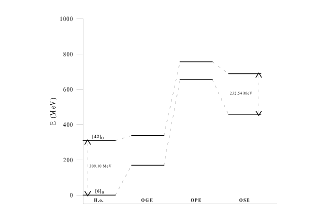
Figure 2: Contribution of the different pieces of the interaction to the energies of the $[42]_{O}$ and $[6]_{O}$ spatial symmetries. Energies are given at R=0.

The chiral potential produces strong repulsion in both cases due mainly to the OPE. In figure 2 it can be seen the effect of the different terms of the interaction. The OGE, repulsive in both configurations, reduces the energy difference whereas the OSE, attractive in both configurations, increases it. The OPE produces a strong repulsion in both symmetries. The net effect is an energy difference of about the same value obtained in the harmonic oscillator but with an additional repulsion in both symmetries originated mainly by quark antisymmetry on the OPE. Therefore, in this type of models the NN $S$-wave hard-core like behaviour should be mainly attributed to the strong repulsion in the $[6]_{O}$ spatial configuration (more precisely there is a compromise between repulsion and kinetic energy difference in both configurations giving rise to some configuration mixing).

These simple images of the origin of the NN short-range repulsion are confirmed by means of explicit RGM or Born-Oppenheimer calculations of the NN relative motion based on OGE [26, 30, 27, 32, 33] or OGE plus Goldstone boson exchanges [42, 43, 74, 47]. Such calculations have been done considering explicitly the NN and $\Delta\Delta$ components (explicit hidden color-hidden color states were considered in Refs. [32, 33]) and the mixing induced between them by the different interactions.

4 The baryon-baryon potential

It has become clear in the last years the major role played by baryonic resonances, in particular the low-lying nucleonic resonances $\Delta$(1232) and N^∗(1440), in many electromagnetic and strong reactions that take place in nucleons and nuclei. This justifies the current experimental effort to study nucleon resonances in several facilities: TJNAF with a specific experimental program of electroexcitation of resonances, WASA in Uppsala to study ${\rm NN}\rightarrow{\rm NN}\pi\pi$ reactions, etc. In this context the knowledge of the interaction involving resonances derived in a consistent way is of great relevance. The interaction between the nucleon and a resonance has been usually written as a straightforward extension of some pieces of the NN potential modifying the coupling constants extracted from their decay widths. Though this procedure can be appropriate for the very long-range part of the interaction, it is under suspicion at least for the short-range part for which the detailed structure of baryons may determine to some extent the form of the interaction. It seems therefore convenient to proceed to a derivation, besides the NN potential which will serve to fix the quark potential parameters, of the $\rm{NN}\rightarrow\rm{NR}$ (R : resonance), $\rm{NR}\rightarrow\rm{NR}$, and $\rm{RR}\rightarrow\rm{RR}$ interactions based on the more elementary quark-quark interaction. The main comparative advantage of the quark treatment comes out from the fact that as all the basic interactions are at the quark level, the parameters of each vertex (coupling constants, cut-off masses,…) are independent of the baryon to which the quarks belong, what makes its generalization to any other non-strange baryonic system straightforward. The other way around, the comparison of its predictions to the experimental data available serves as a stringent test of the quark potential model.

The derivation of the dynamics of a two-baryon system from the dynamics of its constituents is a tough six-body problem whose solution cannot be exactly obtained even for the non-relativistic case. This forces the use of approximate calculation methods. In the literature two methods have been mainly used to get baryonic interactions from the dynamics of the constituents: the resonating group method (RGM) and the Born-Oppenheimer (BO) approximation. We resume their most relevant aspects.

4.1 Calculation methods

4.1.1 Resonating group method potential

The RGM [75], widely used in nuclear physics to study the nucleus-nucleus interaction, can be straightforwardly applied to study the baryon-baryon interaction in the quark model. It allows, once the Hilbert space for the six-body problem has been fixed, to treat the inter-cluster dynamics in an exact way.

The formulation of the RGM for a system of two baryons, $B_{1}$ and $B_{2}$, starts from the wave function of the six-quark system expressed in terms of the Jacobi coordinates of the baryons. Then, the spatial part factorizes in a product of two three-quark cluster wave functions and the relative motion wave function of the two clusters so that,

$$\Psi_{B_{1}B_{2}}={\cal A}\;[\varphi(\vec{P})\;\phi_{B_{1}}(\vec{p}_{\xi_{B_{1}}})\;\phi_{B_{2}}(\vec{p}_{\xi_{B_{2}}})\;\chi_{B_{1}B_{2}}^{ST}\xi_{C}[2^{3}]\,],$$ (4.1)

where ${\cal A}$ is the six-quark antisymmetrizer, $\varphi(\vec{P})$ is the relative motion wave function of the two clusters, $\phi_{B_{i}}(\vec{p}_{\xi_{B_{i}}})$ is the internal momentum wave function of baryon $B_{i}$, and $\xi_{B_{i}}$ are the Jacobi coordinates of the baryon $B_{i}$. $\chi_{B_{1}B_{2}}^{ST}$ denotes the spin-isospin wave function of the two-baryon system coupled to spin $S$ and isospin $T$, and, finally, $\xi_{C}[2^{3}]$ is the product of two colour singlets.

The dynamics of the system is governed by the Schrödinger equation:

$$({\cal H}-E_{T})|\Psi>=0\ \ \ \Rightarrow\ \ \ <\delta\Psi|({\cal H}-E_{T})|\Psi>=0,$$ (4.2)

where

$${\cal H}=\sum_{i=1}^{6}{\vec{p_{i}}^{2}\over 2m_{q}}+\sum_{i<j=1}^{6}V_{qq}(\vec{r}_{ij})-T_{\rm CM}\,,$$ (4.3)

$T_{\rm CM}$ being the center of mass kinetic energy, $V_{qq}$ the quark-quark interaction, $\vec{p_{i}}$ the trimomentum of quark $i$, and $m_{q}$ the constituent quark mass. In equation (4.2) the variations are performed on the unknown relative motion wave function $\varphi(\vec{P})$. Assuming harmonic oscillator wave functions for $\phi_{B_{i}}$ equation (4.2), after the integration of the internal degrees of freedom of both clusters, can be written in the following way [76],

$$\left({\vec{P}^{2}\over 2\mu}-E\right)\varphi(\vec{P})+\int\left(V_{D}(\vec{P},\vec{P}_{i})+W_{\rm EX}(\vec{P},\vec{P}_{i})\right)\varphi(\vec{P})d\vec{P}_{i}=0\,,$$ (4.4)

where $E=E_{T}-E_{B_{1}}-E_{B_{2}}=E_{T}-E_{in}$, $E_{in}$ being the internal energy of the two-body system and $V_{D}(\vec{P},\vec{P}_{i})$ and $W_{\rm EX}(\vec{P},\vec{P}_{i})$ are the direct and exchange RGM kernels, respectively. $V_{D}$ contains the effect of the interaction between baryonic clusters whereas $W_{\rm EX}$ gives account of the quark exchanges between clusters coming from the identity of quarks. They are evaluated in detail in reference [77].

Note that if we do not mind how $V_{D}$ and $W_{\rm EX}$ were derived microscopically, equation (4.4) can be regarded as a general single channel equation of motion including an energy-dependent non-local potential given by the sum of $V_{D}$ and $W_{\rm EX}$. This is the RGM baryon-baryon potential.

4.1.2 Born-Oppenheimer potential

The BO method, also known as adiabatic approximation, has been frequently employed for the study of the nuclear force from the microscopic degrees of freedom [25, 78]. It is based on the assumption that quarks move inside the clusters much faster than the clusters themselves. Then one can integrate out the fast degrees of freedom assuming a fixed position for the center of each cluster obtaining in this way a local potential depending on the distance between the centers of mass of the clusters. The potential is defined in the following way [79],

$$V_{B_{1}B_{2}(L\,S\,T)\rightarrow B_{3}B_{4}(L^{\prime}\,S^{\prime}\,T)}(R)={\cal V}_{L\,S\,T}^{L^{\prime}\,S^{\prime}\,T}(R)\,-\,{\cal V}_{L\,S\,T}^{L^{\prime}\,S^{\prime}\,T}(\infty)\,,$$ (4.5)

where

$${\cal V}_{L\,S\,T}^{L^{\prime}\,S^{\prime}\,T}(R)\,=\,\frac{{\left\langle\Psi_{B_{1}B_{2}}^{L^{\prime}\,S^{\prime}\,T}(\vec{R})\mid\sum_{i<j=1}^{6}V_{qq}({\vec{r}_{ij}})\mid\Psi_{B_{3}B_{4}}^{L\,S\,T}(\vec{R})\right\rangle}}{\sqrt{\left\langle\Psi_{B_{1}B_{2}}^{L^{\prime}\,S^{\prime}\,T}(\vec{R})\mid\Psi_{B_{1}B_{2}}^{L^{\prime}\,S^{\prime}\,T}(\vec{R})\right\rangle}\sqrt{\left\langle\Psi_{B_{3}B_{4}}^{L\,S\,T}(\vec{R})\mid\Psi_{B_{3}B_{4}}^{L\,S\,T}(\vec{R})\right\rangle}}\,,$$ (4.6)

with $\Psi_{B_{i}B_{j}}^{L\,S\,T}(\vec{R})$ given by equation (3.9). The subtraction of ${\cal V}_{L\,S\,T}^{L^{\prime}\,S^{\prime}\,T}(\infty)$ assures that no internal cluster energies enter in the baryon-baryon interacting potential.

4.2 Results

Both methods permit to evaluate the influence of the Pauli principle at the quark level on properties of the baryon-baryon interaction. The main conceptual difference between the resulting interactions is that the BO potential is local while the RGM one is non-local,

$$\eqalign{V^{\rm RGM}_{B_{1}B_{2}\to B_{3}B_{4}}&\equiv V^{\rm RGM}_{B_{1}B_{2}\to B_{3}B_{4}}(R,R^{\prime})\\ V^{\rm BO}_{B_{1}B_{2}\to B_{3}B_{4}}&\equiv V^{\rm BO}_{B_{1}B_{2}\to B_{3}B_{4}}(R)\,.}$$

This means that the $T$ matrix calculated solving a Lippmann-Schwinger equation has a different off-shell behaviour and thus will give different results, the larger the difference the more the particles of the system under consideration explore the off-shell region.

Figure 3: Different diagrams contributing to the NN interaction.

In both cases the calculation of a baryonic potential from the quark dynamics involves, due to the antisymmetry operator, the calculation of many different diagrams that are depicted in figure 3 for the case of the NN interaction. The direct terms are represented by diagrams (a) and (b), whereas quark-exchange terms correspond to diagrams (c)$-$(g). The number in square brackets corresponds to the number of equivalent diagrams that can be constructed (it counts the number of quark pairs which are equivalent to the pair $ij$ singled out in the figure). Diagram (a) cancels almost exactly with the self-energy term ${\cal V}_{L\,S\,T}^{L^{\prime}\,S^{\prime}\,T}(\infty)$, it gives a small contribution at short-range. Diagram (b) generates the asymptotic behaviour of the interaction. The relevance of the quark-exchange terms, diagrams (c)$-$(g), depends on the overlap of the baryon wave functions. They are responsible for the short-range structure of the quark-model-based potential and they vanish when the two baryons do not overlap. Next we present results for the NN, N$\Delta$, $\Delta\Delta$, and NN^∗(1440) systems.

4.2.1 The NN interaction

      

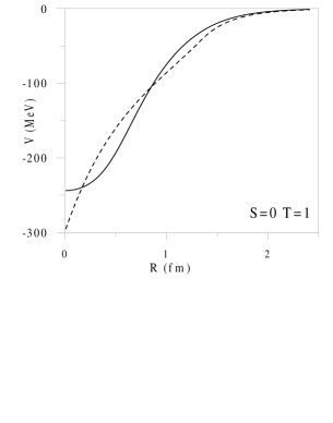
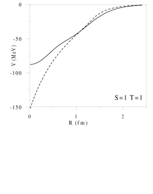
Figure 4: NN OSE potential for two different spin-isospin channels. The dashed line represents the parametrization used in reference [41]. The solid line represents the chiral constituent quark model result [43].

Given the huge amount of experimental data available on the NN system, a detailed calculation of the scattering phase shifts and bound state properties will be presented in section 5. We use this section to discuss qualitative important aspects of the NN interaction that are naturally described in chiral constituent quark models. Let us first mention that the identity of quarks gives rise to the well-known selection rule L+S+T=odd (see section 3.1)

By construction the chiral quark pion potential reproduces the NN long-range interaction (section 2.2). It has been already discussed in section 3.2 how the quark substructure of the nucleon allows to understand the short-range behaviour of the $S$-wave NN interaction. Concerning the medium-range attraction, figure 4 shows the scalar potential obtained in the chiral constituent quark model [43] as compared to a parametrization at baryonic level used in reference [41] to fit the NN experimental data. While at baryonic level different coupling constants are used: $g^{2}_{\sigma\rm{NN}}/4\pi=$ 3.7 for $(S,T)=(0,1)$ and $g^{2}_{\sigma\rm{NN}}/4\pi=$ 1.9 for $(S,T)=(1,1)$, the quark model result is obtained in both cases from the same chiral quark coupling constant. Moreover, the deuteron binding energy is also reproduced [62], while the scalar coupling constant used at baryonic level in this case is once more a different one, $g^{2}_{\sigma\rm{NN}}/4\pi=$ 2.55 [81].

Another important feature of chiral constituent quark models is that although asymptotically the spin-isospin structure of the different terms of the baryon-baryon potential is the same as the corresponding terms of the quark-quark one, at short distances quark exchange generates a rather involved spin-isospin structure. This is due to the antisymmetrization operator, that can be factorized as ${\cal A}\equiv(1-9P_{36})(1-{\cal P})$. When the quark spin-isospin operators are transformed algebraically to find the corresponding baryonic operators different structures are generated [64]. Taking into account that $P^{ST}_{36}={1\over 4}(1+\vec{\sigma}_{3}\cdot\vec{\sigma}_{6})(1+\vec{\tau}_{3}\cdot\vec{\tau}_{6})$, the effective NN interaction can be decomposed as follows,

$$V_{\rm NN}^{(S,T)}=V_{0}(R)+V_{1}(R)\,{\vec{\sigma}}_{B_{1}}\cdot{\vec{\sigma}}_{B_{2}}+V_{2}(R)\,{\vec{\tau}}_{B_{1}}\cdot{\vec{\tau}}_{B_{2}}+V_{3}(R)\,{\vec{\sigma}}_{B_{1}}\cdot{\vec{\sigma}}_{B_{2}}\,{\vec{\tau}}_{B_{1}}\cdot{\vec{\tau}}_{B_{2}}\,,$$ (4.7)

where $V_{i}(R)$ are functions of the interbaryon distance $R$, and $\vec{\sigma}_{B_{i}}$ ($\vec{\tau}_{B_{i}}$) are the spin (isospin) baryonic operators. The $V_{i}(R)$ functions can be obtained from the calculated potential for the different $(S,T)$ channels,

$$\eqalign{V_{0}(R)&={1\over 16}\left[V_{\rm NN}^{(0,0)}(R)+3V_{\rm NN}^{(0,1)}(R)+3V_{\rm NN}^{(1,0)}(R)+9V_{\rm NN}^{(1,1)}(R)\right]\\ V_{1}(R)&={1\over 16}\left[-V_{\rm NN}^{(0,0)}(R)+V_{\rm NN}^{(0,1)}(R)-3V_{\rm NN}^{(1,0)}(R)+3V_{\rm NN}^{(1,1)}(R)\right]\\ V_{2}(R)&={1\over 16}\left[-V_{\rm NN}^{(0,0)}(R)-3V_{\rm NN}^{(0,1)}(R)+V_{\rm NN}^{(1,0)}(R)+3V_{\rm NN}^{(1,1)}(R)\right]\\ V_{3}(R)&={1\over 16}\left[V_{\rm NN}^{(0,0)}(R)-V_{\rm NN}^{(0,1)}(R)-V_{\rm NN}^{(1,0)}(R)+V_{\rm NN}^{(1,1)}(R)\right]}\,.$$

The decomposition (4.7) comes out from any spin-isospin structure of the quark-quark potential. In figure 5 the spin-isospin independent, $V_{0}$, and the spin-isospin dependent, $V_{1}$, $V_{2}$ and $V_{3}$, terms generated by the OSE potential are shown. The main component of the interaction is, as expected, scalar and attractive, however a small spin-isospin dependence appears. This dependence is a completely new feature with respect to the usual scalar exchange at baryon level and may play a significant role in the understanding of different reactions such as the $p(\alpha,\alpha^{\prime})$ or $p(d,d^{\prime})$ [82].

      

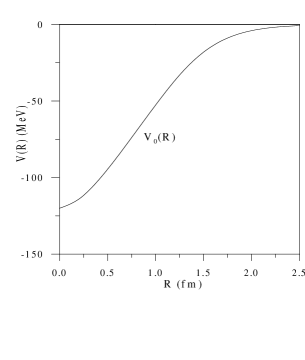
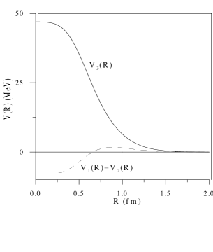
Figure 5: Spin-isospin independent part ($V_{0}$) and spin-isospin dependent parts ($V_{1}$, $V_{2}$, and $V_{3}$) of the OSE potential.

The same decomposition can be applied to the OPE. In this case, the relative strength of the spin-isospin dependent and the tensor terms at the baryonic level is largely reduced with respect to the quark level case, equation (2.5). This allows for a simultaneous explanation of the $p(p,\Delta^{++})n$ and $p(n,p)n$ reactions [58] what is difficult to get when using baryonic meson-exchange potentials [83].

4.2.2 The N$\Delta$ interaction

The inclusion of N$\Delta$ intermediate states has been considered as a possible improvement of NN interaction models at intermediate energies for a long time [84, 85, 86]. The N$\Delta$ interaction has been usually described by means of baryonic meson-exchange models [87] or parametrized by phenomenological potentials [88, 68, 89] with coupling constants and cut-off masses not well determined due to the lack of sufficient experimental information about the N$\Delta$ system.

  

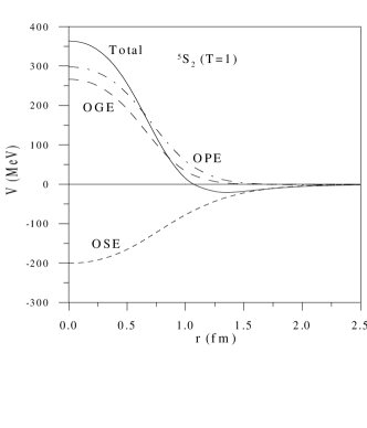
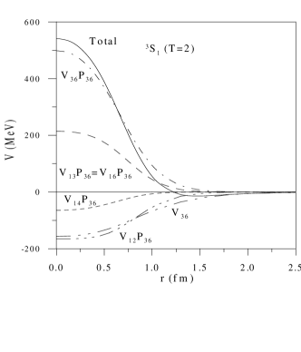
Figure 6: ${}^{5}S_{2}(T=1)$ and ${}^{3}S_{1}(T=2)$ N$\Delta$ potentials.

  

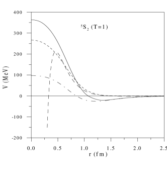
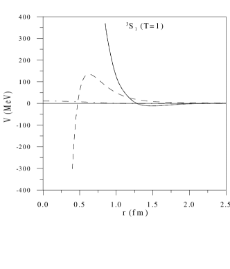
Figure 7: ${}^{5}S_{2}(T=1)$ and ${}^{3}S_{1}(T=1)$ N$\Delta$ potentials. The solid line represents the quark-model based result, the dashed-dotted line the contribution of the OGE and the dotted line that of the OPE+OSE (indistinguishable of the total potential for the ${}^{3}S_{1}(T=1)$ partial wave). The dashed line corresponds to the baryonic meson-exchange potential of reference [87].

Since the $\Delta$ is not a stable particle but rather a $\pi$N resonance, one must establish what it is understood by the N$\Delta$ interaction. The $\Delta$ is considered as an elementary particle, being the coupling to the $\pi$N continuum the responsible for its width [90]. The vicinity of a nucleon modifies the properties of the $\Delta$, because they can exchange particles between each other, eventually a virtual boson. This exchange, which looks like the interaction between two stable particles is what is considered as the N$\Delta$ interaction. The modification by the coupling to the continuum ($\Delta$ width) should be implemented when treating any particular problem.

At the quark level, the N$\Delta$ interaction has been derived in the chiral constituent quark model [66] and used to study the NN system above the pion threshold [91]. Figure 6 shows the N$\Delta$ potential calculated for two partial waves of different isospin, ${}^{5}S_{2}\,(T=1)$ and ${}^{3}S_{1}\,(T=2)$. In one case the contribution of the different terms of the potential has been separated. As in the other case this separation is qualitatively similar, the contribution of the different diagrams of figure 3 is presented. The effect of quark antisymmetrization can be extracted by comparing the total potential with the term $V_{36}$ [diagram (b) in figure 3], the only significant one that does not include quark exchanges. All the exchange diagrams do not appreciably contribute beyond 1.5 fm, where the overlap of the nucleon and $\Delta$ wave functions is negligible. Above this distance the interaction is driven by the $V_{36}$ term and it equals the total interaction. In general, we see how the $V_{12}\,P_{36}$ term [diagram (c)] generates additional attraction and it is the $V_{36}\,P_{36}$ term [diagram (d)] the main responsible for the short-range repulsion. The behaviour of the other diagrams depends on the partial wave considered.

               

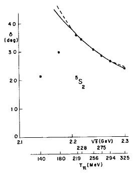
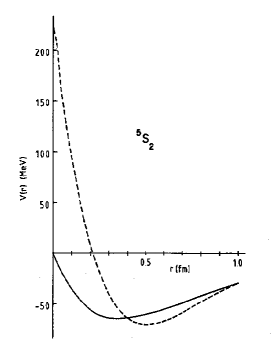
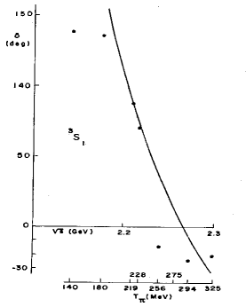
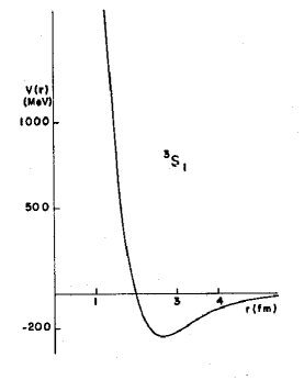
Figure 8: ${}^{3}S_{1}(T=1)$ and ${}^{5}S_{2}(T=1)$ N$\Delta$ phase shifts and separable potentials of reference [68].

 

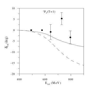
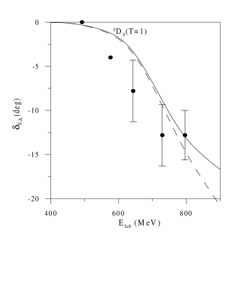
Figure 9: ${}^{3}P_{0}(T=1)$ and ${}^{5}D_{0}(T=1)$ N$\Delta$ phase shifts. The solid line represents the quark model results and the dashed line those of the baryonic meson-exchange model of reference [87]. Experimental data are from reference [92].

In section 3.1 the presence of N$\Delta$ quark Pauli blocked channels, specifically the ${}^{3}S_{1}(T=1)$ and ${}^{5}S_{2}(T=2)$ was discussed. In figure 7 we can see how quark Pauli blocking, existing in the ${}^{3}S_{1}(T=1)$ partial wave, translates into a strong short-range repulsion, while this behaviour is not observed for non-Pauli blocked partial waves as it is the case for the ${}^{5}S_{2}(T=1)$ channel. The strong repulsion is due to the combined effect of the fast decrease of the norm of the six-quark wave function when $R\to 0$ with the presence of non-vanishing direct terms in the potential. Actually, the repulsion manifests itself through the direct contribution of the OPE and OSE potentials. Let us note that if there were no direct contributions, i.e., only quark-exchange diagrams contributed then the resulting behaviour would be quite different since the quark-exchange terms go to zero with the same power of $R$ as the norm.

For the sake of comparison we have also plotted in figure 7 the result for the baryonic meson-exchange model of reference [87]: the strong short-range repulsion does not appear. The only possibility to simulate it would be the use of large cut-off masses, but this would produce instabilities in the short-range part of the interaction. Moreover, the baryonic model gives the same structure in both partial waves, the only difference between them being a spin-isospin factor.

In figure 8, a separable N$\Delta$ potential reproducing the phase shifts (dots in figure 8) obtained from the experimental $\pi d$ elastic cross section is shown [68]. One can infer a hard-core in the ${}^{3}S_{1}(T=1)$ partial wave from the rapidly varying phase shifts changing sign for a pion energy of 219 MeV and a smooth behaviour for the ${}^{5}S_{2}(T=1)$ partial wave. This behaviour is quite similar to the one predicted by the chiral constituent quark model (see figure 7). When not considering the quark substructure a baryon-baryon hard-core has to be introduced by hand to reproduce the experimental data [88, 89].

Nevertheless, potentials are not observable quantities and one should use them to calculate phase shifts to be compared to data, whose extraction is still a matter of controversy. There are a few N$\Delta$ channels which are susceptible of being parametrized in terms of phase shifts. In figure 9 we plot the quark-model result for two uncoupled isospin one N$\Delta$ partial waves, ${}^{3}P_{0}$ and ${}^{5}D_{0}$. Although the error bars are still big, quark-model results agree reasonably well with the experimental data, whereas the baryonic meson-exchange predictions, due to its unsmooth character at short distances [91], are far from the data in the ${}^{3}P_{0}$ case.

4.2.3 The $\Delta\Delta$ interaction

  

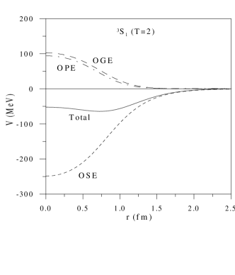
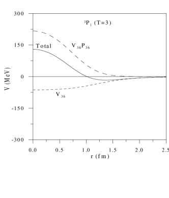
Figure 10: ${}^{3}S_{1}(T=2)$ and ${}^{3}P_{1}(T=3)$ $\Delta\Delta$ potential.

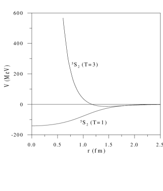
Figure 11: ${}^{5}S_{2}(T=3)$ and ${}^{5}S_{2}(T=1)$ $\Delta\Delta$ potential.

The effect of $\Delta\Delta$ components has been considered when studying NN phase shifts at intermediate energies and deuteron properties at the baryon level [93, 94]. This treatment suffers from the same shortcomings mentioned in the N$\Delta$ case.

At the quark level the two identical baryon selection rule, L+S+T=odd, comes out from quark antisymmetrization. From the chiral constituent quark model potential the $\Delta\Delta$ interaction has been derived in reference [71]. The potential obtained is drawn in figure 10 for two partial waves of different isospin, ${}^{3}S_{1}(T=2)$ and ${}^{3}P_{1}(T=3)$. In one of them the contribution of the different exchanges has been separated and in the other the contribution of the dominant diagrams showed in figure 3 are depicted. As can be seen, the dominant terms are diagrams (b) and (d), the others giving almost a negligible contribution. In both cases the direct contribution, diagram (b), (only generated by quark-meson exchanges) is attractive, while the effect of the quark-exchange diagram (d) (due to quark antisymmetry) is to generate repulsion. Beyond 1.5 fm, the interaction is driven by the $V_{36}$ term that equals the total interaction.

Table 4: Character of the $\Delta\Delta$ interaction obtained in references [79, 95], reference [98], and reference [71]. The ($\star$) denotes those channels where a bound state would be favoured.

• $(S,T)$	Refs. [79, 95]	Ref. [98]	Ref. [71]
  (0,1)	Attractive	$-$	Attractive ($\star$)
  (0,3)	Weakly repulsive	Attractive	Weakly repulsive
  (1,0)	Attractive	Repulsive	Attractive ($\star$)
  (2,3)	Repulsive	$-$	Repulsive
  (3,0)	Attractive ($\star$)	Attractive ($\star$)	Weakly attractive
  (3,2)	Repulsive	$-$	Repulsive

According to the discussion in section 3.1, the ${}^{5}S_{2}(T=3)$, ${}^{7}S_{3}(T=2)$, and ${}^{7}P_{2,3,4}(T=3)$ channels correspond to quark Pauli blocked states. We compare in figure 11 the $\Delta\Delta$ potential for two $S$ waves, a Pauli blocked channel, ${}^{5}S_{2}(T=3)$, and a non-Pauli blocked one, ${}^{5}S_{2}(T=1)$. While the last one presents a soft attractive behaviour at short distances, the ${}^{5}S_{2}(T=3)$ channel shows a strong repulsive core coming from the fast decreasing of the overlapping of the two-baryon wave function (denominator in (4.6)) together with non-vanishing direct terms in the numerator.

It is interesting to analyze the possible existence of bound states with the chiral constituent quark model since this has been the object of study of the $\Delta\Delta$ system with quark models containing confinement plus OGE potentials [79, 95, 96, 97, 98]. In table 4 results of reference [71], based on the chiral constituent quark model, are compared to those of references [79, 95, 98], based on a OGE model. With respect to the possibility of having a favoured bound state in the $(S,T)=(3,0)$ channel, as predicted in [79, 95, 98], reference [71] gets no OGE attraction but repulsion, although as it is shown in the table the total interaction is weakly attractive mainly due to the scalar exchange potential. Reference [71] predicts the $(S,T)=(0,1)$ and $(1,0)$ channels to be the most attractive ones. This attraction, combined with the fact that they are $S$ waves and therefore the centrifugal barrier is not active, makes them the best candidates for possible $\Delta\Delta$ bound states [99], as will be discussed in section 7.2.6.

4.2.4 The NN^∗(1440) system

The N^∗(1440) (Roper) couples strongly (60$-$70$\%$) to the $\pi$N channel and significantly (5$-$10$\%$) to the $\sigma$N channel [100]. Its role in nuclear dynamics as an intermediate state has been analyzed at the baryon level. The presence of NN^∗(1440) configurations in the deuteron was suggested long ago [101, 102, 103, 104]. Graphs involving the excitation of N^∗(1440) appear also in other systems, as for example the neutral pion production in proton-proton reactions [105] or the three-nucleon interaction mediated by $\pi$ and $\sigma$ exchange contributing to the triton binding energy [106]. The excitation of the Roper resonance has also been used to explain the missing energy spectra in the $p(\alpha,\alpha^{\prime})$ reaction [107] or the $np\to d(\pi\pi)^{0}$ reaction [108]. Pion electro- and photoproduction from nucleons may take place through the N^∗(1440) excitation as well [109].

At the quark level the involved N^∗(1440) radial structure increases the number of diagrams contributing to the interaction. There appear diagrams generated by the two parts of the wave function, $\phi_{1}$ and $\phi_{2}$ in equation (3.4). Although involving interactions between excited and non-excited quarks, they can be classified as in figure 3. The full set of diagrams for the NN^∗(1440) potential are explicitly given in [67] and those for the ${\rm NN}\to{\rm NN}^{*}(1440)$ potential in [110].

  

Figure 12: Contribution of the different terms of the interaction to the ${}^{1}S_{0}(T=0)$ and ${}^{1}S_{0}(T=1)$ NN^∗(1440) potentials.

4.2.5 The NN^∗(1440) interaction

In this case we shall classify the channels, for the reason that will be apparent in what follows, as forbidden channels, i.e., allowed in the NN^∗(1440) system but forbidden in the NN case, and allowed channels, i.e., allowed in both NN^∗(1440) and NN systems according to (3.11). In figure 12 the potential for a forbidden channel, ${}^{1}S_{0}$ (T=0), and for an allowed one, ${}^{1}S_{0}$ (T=1), are compared. As can be seen, forbidden channels in $S$ waves are much more repulsive than allowed ones, this repulsion being mainly driven by the non-vanishing direct terms in the potential. Moreover, as detailed in reference [67], the potential for the forbidden ${}^{1}S_{0}(T=0)$ channel is very much the same than for the allowed ${}^{1}P_{1}(T=0)$ and similarly for ${}^{3}S_{1}(T=1)$ and ${}^{3}P_{J}(T=1)$ (in this last case with small dependence on $J$ due to the tensor interaction). This can be understood in terms of the Pauli and the centrifugal barrier repulsions. The Pauli correlations and the centrifugal barrier in the $P$ waves prevent all the quarks to be in the same spatial state, much the same effect one has due to Pauli correlations in the $S$ forbidden waves added to the presence of the radially excited quark in the N^∗(1440).

The lack of available data and the absence of alternative quark model calculations to compare with makes convenient in this case to extract a pure baryonic potential whose difference with the total one emphasizes the effects of the quark substructure. The dynamical effect of quark antisymmetrization can be estimated by comparing the total potential with the one arising from diagram (b) in figure 3, $V_{36}$, which is the only significant one that does not include quark exchanges. The $V_{36}$ potential turns out to be attractive everywhere. Let us note however that Pauli correlations are still present in the $V_{36}$ potential, through the norm, in the denominator of equation (4.6). To eliminate the whole effect of quark antisymmetrization one should eliminate quark-Pauli correlations from the norm as well. By proceeding in this way one gets a genuine baryonic potential, that will be called direct potential. The comparison of the total and direct potentials reflects the quark antisymmetrization effect beyond the one-baryon structure, see figure 13. As $V_{36}$, the direct potential is attractive everywhere. It becomes then clear that the repulsive character of the interaction for $S$ and $P$ waves at short distances is due to dynamical quark-exchange effects. For distances $R\geq$ 2 fm the direct and total potentials are equal since then the overlap of the N and the N^∗(1440) wave functions is negligible and no exchange diagrams contribute appreciably. These results clearly illustrate that the use of a NN^∗(1440) potential as a generalization of the NN interaction should be taken with great care, specially for the forbidden channels.

4.2.6 The NN $\rightarrow$ NN^∗(1440) interaction

The presence of two identical baryons in the initial state forces in this case the selection rule L+S+T=odd. For the ${\rm NN}\rightarrow{\rm NN}^{*}(1440)$ potential, most diagrams contributing to the interaction are due to the first term of the N^∗(1440) wave function (3.4), i.e., $|[3](0s)^{2}(1s)\rangle$.

  

Figure 13: Comparison between the total and direct potentials for ${}^{1}S_{0}(T=0)$ and ${}^{1}S_{0}(T=1)$ NN^∗(1440) potentials.

  

Figure 14: ${}^{1}S_{0}$ and ${}^{3}S_{1}$ $\rm{NN}\to\rm{NN}^{*}(1440)$ potentials. The long-dashed, dashed and dotted lines denote the OPE, OSE and OGE contributions, respectively.

In figure 14, the potentials for ${}^{1}S_{0}$ and ${}^{3}S_{1}$ partial waves are shown (let us note that an arbitrary global phase between the N and N^∗(1440) wave functions has been chosen). Although the long-range part of the interaction ($R>4$ fm ) comes dominated by the OPE, the asymptotic potential reverses sign with respect to both NN and NN^∗(1440) cases. Thus for $S$ and $D$ waves the ${\rm NN}\rightarrow{\rm NN}^{*}(1440)$ interaction is asymptotically repulsive. This sign reversal is a direct consequence of the presence of a node in the N^∗(1440) wave function what implies a change of sign with respect to the N wave function at long distances (for NN^∗(1440) there are two compensating changes of sign coming from the two Ropers). This is also corroborated by the study of the OSE interaction that is always asymptotically repulsive at difference to the NN and NN^∗(1440) cases. If the opposite sign for the N^∗(1440) wave function were chosen the long-range part of the interaction would be attractive but there would also be a change in the character of the short-range part.

It is worth to remark that no quark antisymmetrization effects survive either in the numerator or in the denominator (norm) of equation (4.6) at these distances. In other words, the potential corresponds to a direct baryon-baryon interaction that can be fitted as it is conventional in terms of a Yukawa function depending on the mass of the meson.

The total potential turns out to be attractive from $R=$ 1.5 fm down to a lower value of $R$ different for each partial wave. This behaviour, related again to the node in the Roper wave function, contrasts with the elastic NN and NN^∗(1440) cases, where for instance for $S$ and $D$ waves the scalar part keeps always the same sign and gives the dominant contribution for $R>$0.8 fm. Below 0.6 fm the potential becomes repulsive in all partial waves. Nevertheless there are two distinctive features with respect to the elastic NN and NN^∗(1440) cases: in $\rm{NN}\rightarrow\rm{NN}^{*}(1440)$ the intensity of the repulsion at $R=$0 and the value of $R$ at which the interaction becomes repulsive are significantly lower than in NN and NN^∗(1440) elastic potentials. This is a clear effect of the more similarity (higher overlap) in these cases between initial and final states what makes the Pauli principle more active.

Let us also mention that at short distances, the interaction could be fitted in terms of two different Yukawa functions, one depending on the meson mass, $m$, the other with a shorter range depending on $\sqrt{(M_{{\rm N}^{*}(1440)}-M_{\rm N}+m)m}$. These two Yukawa functions could be associated to the two diagrams with different intermediate states [$m{\rm NN}$ and $m{\rm NN}^{*}(1440)$] appearing in time ordered perturbation theory when an effective calculation at the baryonic level is carried out (let us realize that in a quark calculation the intermediate state is always $mqq$, the N^∗(1440)$-$N mass difference being taken into account through the N and N^∗(1440) wave functions).

4.3 $\pi{\rm NN}^{*}(1440)$ and $\sigma{\rm NN}^{*}(1440)$ coupling constants

A main feature of the quark treatment is its universality in the sense that all baryon-baryon interactions are treated on an equal footing. This allows a microscopic understanding and connection of the different baryon-baryon interactions that is beyond the scope of any analysis based only on effective hadronic degrees of freedom. We will illustrate this discussion by means of the ${\rm NN}\to{\rm NN}^{*}(1440)$ transition potential, determining the $\pi{\rm NN}^{*}(1440)$ and $\sigma{\rm NN}^{*}(1440)$ coupling constants.

As has been discussed in section 4.2.1, asymptotically ($R\geq$4 fm) the OSE and OPE potentials have at the baryon level the same spin-isospin structure than at quark level. Hence one can try to parametrize the asymptotic central interactions as,

$$V_{{\rm NN}\to{\rm NN}^{*}(1440)}^{\rm OPE}(R)=\frac{1}{3}\,\frac{g_{\pi{\rm NN}}}{\sqrt{4\pi}}\,\frac{g_{\pi{\rm NN}^{*}(1440)}}{\sqrt{4\pi}}\,\frac{m_{\pi}}{2M_{N}}\,\frac{m_{\pi}}{2(2M_{r})}\,\frac{\Lambda^{2}}{\Lambda^{2}-m_{\pi}^{2}}$$

$$\hbox to0.0pt{\hss${}[{}$}(\vec{\sigma}_{N}.\vec{\sigma}_{N})(\vec{\tau}_{N}.\vec{\tau}_{N})]\,\frac{e^{-m_{\pi}R}}{R}\,,$$ (4.8)

and

$$V_{{\rm NN}\rightarrow{\rm NN}^{*}(1440)}^{\rm OSE}(R)=-\,\frac{g_{\sigma NN}}{\sqrt{4\pi}}\,\frac{g_{\sigma{\rm NN}^{*}(1440)}}{\sqrt{4\pi}}\,\frac{\Lambda^{2}}{\Lambda^{2}-m_{\sigma}^{2}}\,\frac{e^{-m_{\sigma}R}}{R}\,,$$ (4.9)

where $g_{i}$ stands for the coupling constants at the baryon level and $M_{r}$ is the reduced mass of the NN^∗(1440) system.

By comparing these baryonic potentials with the asymptotic behaviour of the OPE and OSE previously obtained one can extract the $\pi{\rm NN}^{*}(1440)$ and $\sigma{\rm NN}^{*}(1440)$ coupling constants in terms of the elementary $\pi qq$ coupling constant and the one-baryon model dependent structure (see section 2.2). The sign obtained for the meson-NN^∗(1440) coupling constants and for their ratios to the meson-NN coupling constants is ambiguous since it comes determined by the arbitrarily chosen relative sign between the N and N^∗(1440) wave functions. Only the ratios between $\pi{\rm NN}^{*}(1440)$ and $\sigma{\rm NN}^{*}(1440)$ would be free of this uncertainty. This is why only absolute values will be quoted, except for these cases where the sign comes as a prediction of the model. For this study the ${}^{1}S_{0}$ will be used for simplicity. This is why only the central interaction has been written in equation (4.8).

The $\Lambda^{2}/(\Lambda^{2}-m_{i}^{2})$ vertex factor comes from the vertex form factor chosen at momentum space as a square root of monopole $[\Lambda^{2}/(\Lambda^{2}+\vec{q}^{\,2})]^{1/2}$, the same choice taken at the quark level, where chiral symmetry requires the same form for pion and sigma. A different choice for the form factor at the baryon level, regarding its functional form as well as the value of $\Lambda$, would give rise to a different vertex factor and eventually to a different functional form for the asymptotic behaviour. For instance, for a modified monopole form, $[(\Lambda^{2}-m^{2})/(\Lambda^{2}-q^{2})]^{1/2}$, where $m$ is the meson mass ($m_{\pi}$ or $m_{\sigma}$), the vertex factor would be $1$, i.e. $(\Lambda^{2}-m^{2})/(\Lambda^{2}-m^{2})$, keeping the potential the same exponentially decreasing asymptotic form. Then it is clear that the extraction from any model of the meson-baryon-baryon coupling constants depends on this choice. We shall say they depend on the coupling scheme.

  

Figure 15: Asymptotic behaviour of the OPE and OSE ${}^{1}S_{0}$ ${\rm NN}\to{\rm NN}^{*}(1440)$ potential (solid line), the dashed line represents the fitted curves according to (4.8) and (4.9). For the OSE potential both lines are indistinguishable.

For the OPE with $\Lambda=4.2$ fm^-1, $\Lambda^{2}/(\Lambda^{2}-m_{\pi}^{2})=1.03$, pretty close to $1$. As a consequence, in this case the use of this form factor or the modified monopole form at baryonic level makes little difference in the determination of the coupling constant. This fact is used when fixing $g_{\pi qq}^{2}/{4\pi}$ from the experimental value of $g_{\pi{\rm NN}}^{2}/{4\pi}$ extracted from NN data. To get $g_{\pi{\rm NN}^{*}(1440)}/\sqrt{4\pi}$ we turn to the numerical result for the ${}^{1}S_{0}$ OPE potential and fit its asymptotic behaviour (in the range $R:5\to$9 fm, see figure 15) to equation (4.8), obtaining

$$\frac{g_{\pi{\rm NN}}}{\sqrt{4\pi}}\frac{g_{\pi{\rm NN}^{*}(1440)}}{\sqrt{4\pi}}\frac{\Lambda^{2}}{\Lambda^{2}-m_{\pi}^{2}}=\,-\,3.73\,,$$ (4.10)

i.e. $g_{\pi{\rm NN}^{*}(1440)}/\sqrt{4\pi}=-0.94$. As explained above only the absolute value of this coupling constant is well defined. In reference [111] a different sign is obtained what is a direct consequence of the different global sign chosen for the N^∗(1440) wave function. The coupling scheme dependence can be explicitly eliminated comparing $g_{\pi{\rm NN}^{*}(1440)}$ with $g_{\pi{\rm NN}}$ extracted from the NN potential within the same quark model,

$$\left|\frac{g_{\pi{\rm NN}^{*}(1440)}}{g_{\pi{\rm NN}}}\right|=0.25\,.$$ (4.11)

By proceeding in the same way for the OSE potential, i.e. by fitting the potential to equation (4.9), and following an analogous procedure for the NN case one can write

$$\left|\frac{g_{\sigma{\rm NN}^{*}(1440)}}{g_{\sigma{\rm NN}}}\right|=0.47\,.$$ (4.12)

The relative phase chosen for the N^∗(1440) wave function with respect to the N wave function is not experimentally relevant in any two step process comprising N^∗(1440) production and its subsequent decay. However it will play a relevant role in those reactions where the same field ($\pi$ or $\sigma$) couples simultaneously to both systems, NN and NN^∗(1440). In these cases the interference term between both diagrams would determine the magnitude of the cross section [107].

The ratio given in (4.11) is similar to that obtained in reference [111] and a factor 1.5 smaller than the one obtained from the analysis of the partial decay width. Indeed one can find in the literature values for $f_{\pi{\rm NN}^{*}(1440)}$ ranging between 0.27$-$0.47 coming from different experimental analyses with uncertainties associated to the fitting of parameters [108, 112, 109]. Regarding the ratio obtained in (4.12), it agrees quite well with the only experimental available result, obtained in reference [107] from the fit of the cross section of the isoscalar Roper excitation in $p(\alpha,\alpha^{\prime})$ in the 10$-$15 GeV region, where a value of 0.48 is given.

Furthermore, a very definitive prediction of the magnitude and sign of the ratio of the two ratios is obtained,

$$\frac{g_{\pi{\rm NN}^{*}(1440)}}{g_{\pi{\rm NN}}}=0.53\;\frac{g_{\sigma{\rm NN}^{*}(1440)}}{g_{\sigma{\rm NN}}}\,,$$ (4.13)

which is an exportable prediction of the chiral constituent quark model.

For the sake of completeness we give the values of $g_{\sigma{\rm NN}^{*}(1440)}$ and $g_{\sigma{\rm NN}}$, though one should realize that the corresponding form factor ${\Lambda^{2}}/(\Lambda^{2}-m_{\sigma}^{2})=2.97$ differs quite much from 1. Extracting the quark model factor dependence from the coupling constant ($e^{m_{\sigma}^{2}b^{2}/2}$) [67], that one may consider included in the baryon form factor, the results obtained are $g_{\sigma{\rm NN}^{*}(1440)}^{2}/4\pi=$1.14, that compares quite well with the value given in reference [107], $g_{\sigma{\rm NN}^{*}(1440)}^{2}/4\pi=1.33$, and $g_{\sigma{\rm NN}}^{2}/{4\pi}=5.06$. These coupling constants have been also determined in reference [113]. The results reported there are sensitive to the decay width of the sigma into two pions and the mass of the sigma as reflected in the large error bars given. Both quantities are highly undetermined in the Particle Data Book [100], the mass of the sigma being constrained between 400$-$1200 MeV and its width between 600$-$1000 MeV. These values have been fixed in reference [113] to $m_{\sigma}=$500 MeV and $\Gamma_{\sigma}=$250 MeV. Varying the mass of the sigma between 400 and 700 MeV for a fixed width of 250 MeV, the coupling constant according to equation (9) of reference [113] varies between 0.18$-$2.54. Taking a width of 450 MeV the resulting coupling is 0.27$-$1.64. In both cases, our values may be compatible with the N^∗(1440) decay and production phenomenology.

5 The NN system

The most accurate description of NN scattering data and deuteron properties has been done in terms of boson exchanges at the baryon level in the framework of the old-fashioned time ordered perturbation theory, viz., the Bonn potential [114]. On a microscopic base different approaches have attempted to describe the NN interaction. Effective theories are very efficient to reproduce the high orbital angular momentum $(L)$ partial waves but for low $L$ they need to introduce a large number of parameters (more than twenty in reference [115]). Bag models found severe problems in describing the two-baryon dynamics due, on the one hand, to the critical difficulty of separating the center of mass motion and, on the other hand, to the unphysical sharp boundary of the bag and the problem of how to connect six-quark dynamics with external NN dynamics. In the so-called hybrid model approaches short-range dynamics based on the quark substructure combines with a long-range part given by either meson exchanges at the baryonic level (for example references [116] and [117] used the long-range interaction from the one- and two-pion exchange Paris potential [118]) or phenomenological potentials fitted to the experimental data [119]. Although they had a relative success in reproducing the phase shifts these hybrid models are not fully consistent.

Chiral constituent quark models allow to incorporate the medium and long-range dynamics from the quark substructure in a natural way. They were first applied to the non-strange baryon-baryon interaction [42, 43] and later on to derive the potential between all members of the baryon octet [47]. In the last case the model parameters for the exchange of the two pseudoscalars (pion and kaon) and the full scalar and vector octet mesons were independently fitted to the experimental data. This procedure, although very effective to fit the data, does explicitly break the chiral construction of the potential and masks on the model parameters some important physical effects, like the coupling to N$\Delta$ channels [120]. In the following we will refer to the model of reference [43], that has been detailed in section 2, although we will use results of the quark model approach of Ref. [47] for comparison.

5.1 Low-energy scattering parameters and deuteron properties

The scattering length and the effective range provide a useful way to parametrize information on low-energy NN scattering because they are extremely sensitive to small variations on the strength of the NN force. Furthermore, these parameters can be related to other observables such as the deuteron binding energy. Therefore, the correct prediction of the scattering length, the effective range and the deuteron properties should be the first test for any model of the NN system to satisfy. Table 5 resumes the results obtained by means of the chiral constituent quark model [80] compared to the quark model approach of Ref. [121] and some standard NN potentials [114, 122] and experimental data. For a correct description of the ${}^{1}S_{0}$ observables it is necessary to take into account the coupling to the ${}^{5}D_{0}$ ${\rm N}\Delta$ channel, which provides an isospin-dependent mechanism generating additional attraction. Hence a similitude between the ${}^{1}S_{0}$ and the ${}^{3}S_{1}$ NN partial waves, both getting the necessary attraction by the tensor coupling to a $D$ wave (${}^{3}D_{1}$ for ${}^{3}S_{1}$) [120] comes out. Besides it is worth to mention that the description of the low-energy scattering parameters requires a charge symmetry breaking term [114, 123] that has been taken into account by a slight modification of the chiral coupling constant. In the same table the results for the deuteron properties are shown, presenting a good agreement with the experimental data.

Table 5: NN properties. $a_{s(t)}$ is the singlet (triplet) scattering length and $r_{s(t)}$ is the singlet (triplet) effective range. $E_{d}$ is the deuteron binding energy, $P_{D}$ the $D-$state probability, $Q_{d}$ the quadrupole moment, $A_{S}$ the asymptotic $S$-state normalization, and $\eta$ the $D/S$-state ratio.

		CCQM [80]	Ref. [121]	Nijm II [122]	Bonn B[114]	Exp.
Low-energy scattering parameters
${}^{1}S_{0}$	$a_{s}$ (fm)	$-$23.759	$-$23.76	$-$23.739	$-$23.750	$-$23.74$\pm$0.02
	$r_{s}$ (fm)	2.68	2.58	2.67	2.71	2.77$\pm$0.05
${}^{3}S_{1}$	$a_{t}$ (fm)	5.461	5.399	5.418	5.424	5.419$\pm$0.007
	$r_{t}$ (fm)	1.820	1.730	1.753	1.761	1.753$\pm$0.008
Deuteron properties
$E_{d}$ (MeV)		$-$2.2242	$-$2.225	$-$2.2246	$-$2.2246	$-$2.224575
$P_{D}$ ($\%$)		4.85	5.49	5.64	4.99	$-$
$Q_{d}$ (fm2)		0.276	0.270	0.271	0.278	0.2859$\pm$0.0003
$A_{S}$ (fm-1/2)		0.891	$-$	0.8845	0.8860	0.8846$\pm$0.0009
$\eta$		0.0257	0.0253	0.0252	0.0264	0.0256$\pm$0.0004

5.2 Deuteron configurations

Although the deuteron has been usually described as a NN isospin singlet in even partial waves, i.e., ${}^{3}S_{1}$ and ${}^{3}D_{1}$, it could also be understood as a linear combination of pairs of baryonic resonances provided they have the adequate quantum numbers. Such a description finds its natural framework in quark models for two reasons. First, from a quark model point of view baryon resonances are no more than internally excited nucleons. These excitations may occur even at low energies due to the virtual process ${\rm NN}\to{\rm NN}^{*}({\rm N}^{*}{\rm N}^{*})\to{\rm NN}$ involving intermediate N^∗’s. Second, all baryon-baryon interactions can be generated from the same underlying quark-quark potential and, therefore, described in a consistent way. Furthermore, the presence of colour for the quarks adds the possibility of having new exotic components such as hidden colour state configurations: two colour octets coupled to a singlet. Although in some works their contribution to the deuteron wave function has been found to be as large as $5\%$ [124], it is possible to demonstrate that any hidden colour state can be expressed as a linear combination of physical states, i.e., baryon-baryon states [125].

The most prominent low-lying even-parity nucleon resonances are the $\Delta$ and the N^∗(1440). Being the deuteron isoscalar the N$\Delta$ configuration is forbidden and therefore $\Delta\Delta$ and NN^∗(1440) components would be the relevant non-nucleonic configurations. For the $\Delta\Delta$ configuration, reference [93] established a significant upper limit of about $0.4\%$. Moreover, although there are no experimental data on the NN^∗(1440) configuration, this has been advocated long ago to understand elastic proton-deuteron backward scattering at energies above pion threshold [126] or the angular distribution of deuteron photodisintegration at energies above $E_{\gamma}=$ 100 MeV [127]. Recent calculations have renewed the interest on these non-nucleonic components as they could be indirectly observed in several reactions as for example antiproton-deuteron annihilation [128], subthreshold antiproton production [129] or $pd\to dp$ processes [130].

Table 6: Probability of the different deuteron components ($\%$)

• NN		NN∗(1440)		$\Delta\Delta$
  ${}^{3}S_{1}$	${}^{3}D_{1}$	${}^{3}S_{1}$	${}^{3}D_{1}$	${}^{3}S_{1}$	${}^{3}D_{1}$	${}^{7}D_{1}$	${}^{7}G_{1}$
  95.3780	4.6220	$-$	$-$	$-$	$-$	$-$	$-$
  95.1989	4.5606	$-$	$-$	0.1064	0.0035	0.1243	0.0063
  95.1885	4.5377	0.0022	0.0148	0.1224	0.0036	0.1245	0.0063

There are several deuteron multichannel calculations using different approximations. Reference [131] proposed a formulation in terms of quark-shell configurations, later on projected onto physical channels. Reference [132] studied the effective numbers for different resonance configurations making use of baryon wave functions obtained from the diagonalization of a quark-quark interaction containing gluon and pion exchanges in a harmonic oscillator basis including up to 2$\hbar\omega$ excitations, and deuteron wave functions obtained from the Paris potential. An upper limit of $1\%$ for $\Delta\Delta$ components and $0.1\%$ for NN^∗(1440) was obtained. Possible effects of six-quark bags at short-distances were considered in [133]. In reference [134] the influence of N and $\Delta$ resonances on the NN interaction was studied. The most significant contribution was inferred from channels involving N and $\Delta$ ground states, although a quantitative calculation of the non-nucleonic configurations was not performed.

The most complete multichannel calculation was done in [135] and [136] using a chiral constituent quark model. The different configurations and partial waves included in the calculation are shown in table 6 together with their probabilities (for instance the first row contains only the NN configurations ${}^{3}S_{1}$ and ${}^{3}D_{1}$). In all cases the deuteron binding energy is correctly reproduced, being $E_{d}=-$2.2246 MeV. The first remarkable result (the last row of table 6) is that the probabilities of NN^∗(1440) channels are smaller than the $\Delta\Delta$ ones being these later ones compatible with the experimental limits given in [93]. As compared to other values in the literature, the total probability of $\Delta\Delta$ components is three times smaller than the one reported in [137], although presenting the same distribution with respect to the different channels. Regarding the calculations of reference [138], a similar distribution is obtained but the total probability being twice as much. Nonetheless, the comparison with these results should be done with care. For example, reference [137] carries out a coupled-channel calculation using for the ${\rm NN}\to\Delta\Delta$ transition potential a combination of $\pi$ and $\rho$ exchanges, and the Reid soft core potential for the rest. Such calculations are not fully consistent since they use NN potentials (Reid soft core or Paris) which were designed, in principle, without explicit $\Delta$ degrees of freedom. Therefore, parts of the contribution from the $\Delta$ degrees of freedom are implicitly included in the parameterization of the potentials.

Regarding the NN^∗(1440) probabilities, they show a larger component of the ${}^{3}D_{1}$ partial wave against the ${}^{3}S_{1}$ partial wave, in agreement with the ordering obtained by other calculations [104, 134]. This can be understood taking into account that the tensor coupling, which is the main responsible for the presence of non-nucleonic components on the deuteron, is much stronger for the ${}^{3}S_{1}({\rm NN})\to\!^{3}D_{1}[{\rm NN}^{*}(1440)]$ transition than for the ${}^{3}D_{1}({\rm NN})\to\!^{3}S_{1}[{\rm NN}^{*}(1440)]$ one, enhancing in this way the $D$-wave influence with respect to the $S$-wave component. Concerning the absolute value of the probabilities, they are a factor ten smaller than those reported in reference [104], where an estimation of 0.17$\%$ for the NN^∗(1440) configuration was obtained (0.06$\%$ for the ${}^{3}S_{1}$ and 0.11 $\%$ for the ${}^{3}D_{1}$ partial wave). The difference with the result of the chiral constituent quark model may be understood in the following way. The deuteron is calculated using the NN Reid hard-core potential. When including NN^∗(1440) components, the channel coupling induces an attractive interaction on the NN system that needs to be subtracted out. Such a subtraction is done by reducing the intermediate range attraction of the central part of the Reid hard-core potential without modifying the tensor part (as done in reference [139] to calculate the probability of $\Delta\Delta$ components). So, the strength of the tensor coupling to the NN^∗(1440) state is not strongly constrained. In fact, a variation of this strength may be compensated by a corresponding modification of the intermediate range attraction. Thus, the balance of these two sources of attraction cannot be disentangled in a clearcut way. This is a similar problem to the one arising in the ${}^{1}S_{0}$ NN partial wave when the coupling to the N$\Delta$ system is included. The same attractive effect may be obtained by a central potential or by a tensor coupling to a state with larger mass, being necessary other observables to discriminate between the two processes [140].

 

Figure 16: Momentum distribution for the ${}^{3}S_{1}({\rm NN})$ and the ${}^{3}S_{1}(\Delta\Delta)$ channels.

Although the probability of $\Delta\Delta$ components is small, its influence for some specific observables can be important. Figure 16 shows the momentum distribution $k^{2}\eta(k)$ ($\eta(k)=|\Psi(k)|^{2}$ is the probability density in momentum space) for the $S$-wave deuteron components. For the ${}^{3}S_{1}({\rm NN})$ case, the solid line represents the results including all NN and $\Delta\Delta$ partial waves while the dashed line refers to the calculation only with NN channels. For the ${}^{3}S_{1}(\Delta\Delta)$ case the dotted line represents the result obtained with all NN channels and only the ${}^{3}S_{1}(\Delta\Delta)$ partial wave, while the dashed line includes all NN channels and the most important $\Delta\Delta$ partial waves, ${}^{3}S_{1}$ and ${}^{7}D_{1}$, being almost identical to the full calculation. As can be observed, the $\Delta\Delta$ components extend to higher momenta regions. This may influence the structure function $B(q)$ which presents a zero for momentum around 7.1 fm^-1. Including only NN components, this result always comes lower, being the $\Delta\Delta$ component a possible candidate to solve the problem [138, 141].

 

Figure 17: ${}^{1}S_{0}$ and ${}^{3}S_{1}$ NN phase shifts.

5.3 NN phase shifts

A calculation of the NN phase shifts below the pion threshold is presented in this section. It includes coupling to $\Delta\Delta$ channels for iso-singlet ($T=0$) partial waves, and to N$\Delta$ and $\Delta\Delta$ channels for iso-triplet ($T=1$) partial waves. Experimental data have been obtained through the interactive program SAID [142] corresponding to the neutron-proton solution SP98.

For the discussion of the results the phase shifts are divided into three groups. First, the $L=0$ partial waves. They are the most sensitive to the short-range part of the interaction and therefore one would expect that quark-exchange effects played for them an important role. A second group will be $P$, $D$ and $F$ waves. They are still sensitive to the short-range part and therefore to quark exchanges, but the middle-range and spin-orbit terms will also play a relevant role. Finally, those partial waves with orbital angular momentum $L>3$ depend basically on the long-range part of the interaction. Although quark exchanges are not expected to be relevant for them, the correct description of these phase shifts supposes a crucial test to the chiral symmetry hypothesis used to derive the basic quark-quark interaction.

5.3.1 S partial waves

   

Figure 18: ${}^{1}P_{1}$ and ${}^{3}P_{J}$ NN phase shifts.

Figure 17 shows the results for the ${}^{1}S_{0}$ and ${}^{3}S_{1}$ partial waves. A perfect fit is obtained for ${}^{1}S_{0}$ up to 250 MeV laboratory kinetic energy and up to 300 MeV for ${}^{3}S_{1}$. As can be checked, the chiral components of the NN interaction (dashed line) do not provide enough attraction to reproduce the experimental data. As previously mentioned, in the ${}^{1}S_{0}$ channel the required attraction is supplied by addition of a coupling to the ${}^{5}D_{0}$ ${\rm N}\Delta$ channel (dotted line). A complete agreement with the experimental data is obtained when the coupling to $\Delta\Delta$ channels is included (solid line). This result shows that the requirements of chiral symmetry (the presence and parameters of the scalar exchange between quarks) are fulfilled by the data provided that one includes the necessary additional physics into the problem.

For the iso-triplet partial wave ${}^{3}S_{1}$, the coupling to $\Delta\Delta$ channels has a smaller influence on the phase shift as can be seen on the figure, and can be simulated by a fine tuning of the mass of the scalar boson [135].

Let us emphasize that it is the strong spin-isospin independent repulsion generated by quark antisymmetry effects on the OPE what allows to reproduce the behaviour of the $S$-wave phase shifts.

5.3.2 P, D and F partial waves

   

Figure 19: Some D and F NN phase shifts.

Among the four $L=1$ partial waves, only the ${}^{1}P_{1}$ is not affected by the spin-orbit interaction. As seen in figure 18 the chiral constituent quark model result (solid line) is in perfect agreement with the experimental data. It is interesting to notice that for this partial wave quark-exchange effects still play an important role. Indeed, in the same figure, the calculation done by removing the terms coming from quark antisymmetry is shown (dashed-dotted line), and the phase shift becomes attractive. This result is easily understood in terms of the direct OPE interaction (the dominant OGE interaction coming from the spin-spin term does not contribute to $P$-waves because of its $\delta$-like behaviour). At short-range the direct OPE potential is repulsive for $S$ waves, but it is attractive for the ${}^{1}P_{1}$ wave due to the different sign of the spin-isospin matrix element. Only when quark antisymmetry terms are considered the OPE produces the correct experimental behaviour.

   

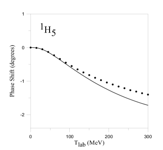
Figure 20: $J=5$ NN phase shifts.

In the same figure the ${}^{3}P_{J}$ triplet phase shifts are shown (notation as in figure 17). One observes, as has been explained for $S$-waves, how the coupling to $\Delta\Delta$ channels in higher angular momentum iso-triplet partial waves is very small. The coupling to N$\Delta$ channels does not improve the description. The failure to reproduce the data may be associated to the lack of spin-orbit interaction.

Some selected $D$ waves are shown in figure 19 (notation as in figure 17). As a general trend, one can say that the model gives too much attraction, except for the ${}^{3}D_{1}$ partial wave where the experimental phase shifts are perfectly reproduced. While for iso-triplet partial waves the coupling to N$\Delta$ channels is still important (worsening the quality of the results), the coupling to $\Delta\Delta$ channels does not produce any considerable effect. For the ${}^{1}D_{2}$ partial wave the result obtained switching off the antisymmetry effects is again displayed by a dashed-dotted line, showing clearly how the influence of antisymmetry diminishes as compared to $S$ and $P$ waves. It is important to note that the $D$-waves are correctly reproduced up to about 80-100 MeV, which may be considered as the characteristic window where the NN interaction is basically governed by chiral symmetry [143]. Higher energies require an improvement in the description of short-range effects, as could be the spin-orbit force which still plays an important role for $D$ waves.

The same figure 19 includes some selected $F$-wave phase shifts. In general there is a better agreement than in $D$-waves up to higher energies of 150-200 MeV. For iso-triplet partial waves the coupling to N$\Delta$ channels produces too much attraction, as it was the case for $P$ and $D$ waves, but the description is of the same quality as that of effective theories [144, 143]. A comment about the ${}^{3}F_{2}$ phase shift is in order. This wave is coupled to the ${}^{3}P_{2}$ wave, which has a strong influence of the spin-orbit interaction. The spin-orbit interaction is attractive for the ${}^{3}P_{2}$ wave and repulsive for the ${}^{3}F_{2}$. Therefore, one expects that when the ${}^{3}P_{2}$ wave approaches the experimental data, the ${}^{3}F_{2}$ will also do the same.

5.3.3 G, H and I partial waves

   

Figure 21: Mixing parameters.

In figure 20 $J=5$ $G$, $H$ and $I$ phase shifts are shown (notation as in figure 17). The results obtained are in good agreement with the experimental data, being fundamentally dominated by the interaction of chiral origin. Iso-triplet partial waves show that the coupling to N$\Delta$ channels, so important for low orbital angular momenta, becomes smaller but contributes to improve the results. Once again they are similar to those obtained by effective theories [144, 143], indicating that these waves are governed exclusively by chiral symmetry.

5.3.4 Mixing parameters

Figure 21 shows the mixing parameters for the tensor coupling between different NN partial waves: ${}^{3}S_{1}-{}^{3}\!D_{1}$, ${}^{3}P_{2}-{}^{3}\!F_{2}$, ${}^{3}D_{3}-{}^{3}\!G_{3}$ and ${}^{3}G_{5}-{}^{3}\!I_{5}$. The dashed line shows the results when only NN components are included. As can be seen, $\epsilon_{1}$ (which represents the tensor coupling ${}^{3}S_{1}-{}^{3}\!D_{1}$) and $\epsilon_{2}$ (which represents the tensor coupling ${}^{3}P_{2}-{}^{3}\!F_{2}$) are not correctly reproduced. For $\epsilon_{2}$ one cannot draw any definite conclusion, because the model does not accurately describe the ${}^{3}P_{2}$ and ${}^{3}F_{2}$ phase shifts. However, despite the very good description of the ${}^{3}S_{1}$ and ${}^{3}D_{1}$ phase shifts, $\epsilon_{1}$ has the correct behaviour only at very low energies. This seems to indicate the need for a stronger short-range tensor force. Such interaction might be obtained from a simultaneous exchange of pions and gluons between quarks [145]. Higher angular momentum mixing parameters are governed by the OPE tensor term and present a good agreement with the experimental data.

5.3.5 Alternative quark model approaches

Other constituent quark model approaches have been used to describe the NN dynamics. Ref. [74] used a generalized chiral symmetry restoration scheme giving rise to four chiral fields instead of the simple image of the $\pi$ and $\sigma$ mesons. Similar results to the ones presented here are obtained. In Refs [47, 48, 121] Fujiwara and collaborators have performed a complete analysis of the NN scattering phase shifts and mixing coefficients. Their quark model approach incorporates a non-relativistic kinetic energy term, a quadratic confinement potential, the full Fermi-Breit interaction with explicit quark-mass dependence and the full octet of scalar and pseudoscalar meson-exchange potentials between quarks. A refined version of the model considered also vector meson-exchange potentials and the momentum-dependent Bryan-Scott term in the scalar and vector meson potentials. An impressive good agreement with the experimental data has been obtained for almost all partial waves and also for the mixing coefficients. However consistency with the one-body problem is lost (see also section 7.3). The main difference with respect to the CCQM used here comes from the presence in the CCQM of a form factor as a consequence of the momentum dependent constituent quark mass generated by chiral symmetry breaking, Eq. (2.3), that allows to regularize the non-central contributions of the OPE without resorting to multiple meson exchanges as in Refs. [47, 48, 121]. In fact, in these works an important contribution from the non-central terms of the octet meson-exchange potential is obtained. In particular, the quadratic spin-orbit component cancels the strong one-pion tensor force. The interest reader could find a detailed description in the quoted works.

5.4 The NN spin-orbit force

The study of $P$ and $D$ phase shifts makes evident a lack of spin-orbit interaction in chiral constituent quark models. The origin of the spin-orbit force is a long-standing problem of the quark model in its description of the NN interaction and the baryon spectrum [147, 41, 52, 149, 148, 146, 19, 64]. On the one hand the spin-orbit force is known to be short ranged and thus a priori it may seem easy to understand on a quark model scheme, but on the other hand, it is a relativistic correction and therefore difficult a priori to accommodate in a non-relativistic approach. In baryonic meson-exchange models [150, 114] the spin-orbit force has its origin on the $\omega$-meson exchange, also responsible for the short-range repulsion. In quark models the inclusion of vector meson exchanges between quarks belonging to different clusters provide contributions similar to the quark-exchange mechanism and would lead to double counting [57], as explained in section 2.1. Therefore, vector mesons are not included and one has to look for a different source of the spin-orbit force.

The non-relativistic reduction of the one-gluon exchange diagram provides at $(p_{q}/m_{q})^{2}$ order two different types of spin-orbit terms, a Galilei invariant (symmetric) term and a Galilei non-invariant (antisymmetric) term. The Galilei-invariant spin-orbit term has received considerable attention in the literature [147, 41, 148, 151, 149], because it presents the same structure as the standard spin-orbit interaction between nucleons. Using this source of spin-orbit force it was demonstrated in reference [151] that it is possible to reproduce the observed spin-orbit splitting in the NN interaction using a large quark-gluon coupling constant $\alpha_{s}\sim 1.6$. However, an effective meson-exchange potential between nucleons and not between quarks was used. When quark-meson exchange is incorporated instead, $\alpha_{s}$ is considerably reduced and the resulting spin-orbit force is not large enough to reproduce the experimental $P$-wave splittings. In fact, when gluon and pion exchange are consistently treated at the quark level, the OGE spin-orbit force has to be multiplied by some numerical factor (usually between 5$-$12 depending on the set of parameters [41, 43, 152]) in order to reproduce the experimental splittings in the NN phase shifts, with the counterpart that it severely disturbs the description of the excited negative-parity baryon spectrum [151, 19]. Regarding the antisymmetric spin-orbit OGE term, the strength of the full triplet-odd NN spin-orbit potential is greatly reduced and its sign may be even reversed when considered. This is the reason why it has not been usually considered in the literature, although there is no fundamental reason to justify this.

Another source of spin-orbit force in chiral constituent quark models is the scalar exchange. In reference [73] it was shown that it is not enough to explain the experimentally observed effects. The strength of the NN one-sigma exchange spin-orbit force (OSE-LS) can be compared to the one-gluon exchange symmetric spin-orbit force (OGE-LS) in the adiabatic approximation. Figure 22 shows the radial part of the NN adiabatic spin-orbit potential for ${}^{3}P_{J}$ and ${}^{3}D_{J}$ waves.

      

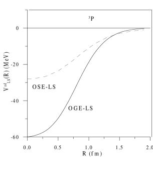
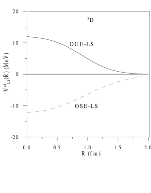
Figure 22: The adiabatic OGE and OSE spin-orbit potential of reference [73] for ${}^{3}P_{J}$ and ${}^{3}D_{J}$ partial waves.

The OGE-LS is generated only by quark-exchange diagrams what makes it highly non-local, while the OSE-LS has a non-vanishing direct term making it longer-ranged. The sign of the OSE-LS is the same for $P$ and $D$ waves, because the direct term dominates. However, the OGE-LS force has a different sign for $P$ and $D$ partial waves, since only the exchange terms contribute.

Finally, the spin-orbit potential generated by confinement is strongly dependent on the particular confinement model. For example, while the symmetric spin-orbit term associated with a scalar two-body confinement potential cancels the OGE symmetric spin-orbit force in the NN interaction [52], the one coming from a flip-flop confinement interaction interferes constructively with it in $P$ waves [149]. For $D$-waves they almost cancel each other, which seems to be consistent with the fact that the NN spin-orbit force is known to be very small for even orbital angular momentum channels. In reference [146], the uncertainties associated with spin-orbit terms generated by quark confinement have been emphasized by studying an alternative model in which confinement is described through a mass term in the relativistic single particle equation. The single particle Thomas term of such a model yields a NN spin-orbit interaction with opposite sign to the one generated by a scalar two-body confining potential. In summary contributions which are usually neglected (antisymmetric spin-orbit terms, Thomas precession terms, etc.) might be even more important than those considered [65].

5.5 Charge dependence of nuclear forces

The possibility of isospin violation in the strong interaction endures as one of the intriguing and partially unsolved aspects in the description of nuclear forces [153]. After electromagnetic effects are removed from the experimental data, small but significant differences exist among the neutron-neutron and proton-proton interactions (charge symmetry breaking, CSB), and among the average of these two interactions and the neutron-proton one (charge independence breaking, CIB). Explicitly in terms of the scattering lengths,

$$\eqalign{\Delta a_{\rm CSB}&=a_{\rm pp}-a_{\rm nn}=1.5\pm 0.5\,{\rm fm}\\ \Delta a_{\rm CIB}&={1\over 2}\left(a_{\rm pp}+a_{\rm nn}\right)-a_{\rm pn}=5.7\pm 0.5\,{\rm fm}\,.}$$ (5.1)

Most of the theoretical calculations to understand these numbers have been done using baryonic meson-exchange models that incorporate basically isospin breaking through the charged and neutral pion mass difference, the proton-neutron mass difference, the $\rho^{0}-\omega$ electromagnetic mixing amplitude, and the electromagnetic corrections. Whilst the major part of the CIB has been explained by means of the mass difference between the neutral and charged pions, proton-neutron mass difference and $\rho^{0}-\omega$ mixing have been used to account for most part of the CSB effects.

From a more fundamental point of view one would expect that the source of $\Delta a_{\rm CIB}$ and $\Delta a_{\rm CSB}$ could be ultimately traced to CIB and CSB in QCD. The traditional quark-model approach incorporates only two sources of isospin breaking, namely up-down quark mass difference and the quark-exchange Coulomb interaction. Chiral constituent quark models incorporate two additional mechanisms contributing to isospin violation, the mass difference between the charged and neutral pion and the leading order electromagnetic loop corrections to the OGE potential (QED-QCD) [154]. All these contributions have been evaluated in reference [123] and the results are shown in table 7. Taking into account the pion-mass splitting ($V^{C}_{\rm OPE}$ and $V^{T}_{\rm OPE}$), the quark-exchange Coulomb interaction ($V_{\gamma}$) and the QED-QCD interference terms ($V_{\rm QED-QCD}$) it is possible to reproduce CIB on the ${}^{1}S_{0}$ scattering length without introducing any additional parameter to those necessary for describing the NN interaction. The contribution of the quark-exchange Coulomb interaction and the QED-QCD interference terms make also possible to explain CSB on the ${}^{1}S_{0}$ scattering length. The influence of up-down constituent quark-mass difference is small due to the cancellation among different terms.

Table 7: Different contributions to $\Delta a_{\rm CIB}$ and $\Delta a_{\rm CSB}$. The number between parenthesis is calculated including the contribution of CSB. $\times$ indicates the contributions considered.

• $V_{\rm OPE}^{C}$	$V_{\rm OPE}^{T}$	$V_{\rm QED-QCD}$	$V_{\gamma}$	$\Delta a_{\rm CIB}\,({\rm fm})$	$\Delta a_{\rm CSB}\,({\rm fm})$
  $\times$	$-$	$-$	$-$	3.07	$-$
  $\times$	$\times$	$-$	$-$	3.41	$-$
  $\times$	$\times$	$\times$	$-$	5.59	$-$
  $\times$	$\times$	$\times$	$\times$	5.97 (5.94)	$-$
  $-$	$-$	$-$	$\times$	$-$	0.26
  $-$	$-$	$\times$	$-$	$-$	1.20
  $-$	$-$	$\times$	$\times$	$-$	1.46

5.6 The NN system above the pion threshold

Figure 23: Contributions of intermediate $\pi$NN states. The pion is drawn as a dashed line, the nucleon and $\Delta$ as single and double solid lines, respectively.

Above the pion production energy the NN experimental data show several structures which cannot be described by simple extrapolation of models explaining the NN data below this energy. To correctly treat the problem it is necessary to incorporate the description of $\pi$NN states. One possible way of treating the $\pi$NN system is by means of explicit nucleon-resonance channels. The three-body problem is then reduced to a two-body problem assuming that the NN$\rightarrow\pi$NN transition only takes place trough resonances. Once the decay width of the resonances is incorporated in the propagators, the equations are able to properly couple physical two (NN) and three ($\pi$NN) particle states. The effect of the coupling to resonances mainly depends on the strength and range of the transition potential. Therefore it is important to use a consistent interaction for the NN and nucleon-resonance channels.

Experimentally it is known that the inelasticity in two-nucleon scattering up to at least 500 MeV in the c.m. system, i.e., far beyond the two-pion threshold, is predominantly due to single-pion production and it occurs essentially in the isospin-triplet partial waves, what suggests that pion production proceeds through single-$\Delta$ excitation. This restriction is an enormous technical simplification [155] and allows to model the $\pi$NN system by means of a NN$-$N$\Delta$ coupled channel problem.

Figure 24: ${}^{1}S_{0}$ NN phase shift and inelasticity.

The main process for pion production is given by the $\pi$N$\Delta$ vertex depicted in figure 23(a), in which the $\Delta$ couples to a $\pi$N state. The introduction of this diagram has two consequences. The first one is that the OPE N$\Delta$ potential has a retarded interaction, shown in figure 23(b), which modifies the $\Delta\Delta$ interaction. However, the diagonal $\Delta\Delta$ potential has a minor influence on the NN channels and usually this modification is not taken into account. The second one is the appearance of the delta self-energy diagram in the presence of a spectator nucleon shown in figure 23(c), that has a contribution to the $\Delta$ width and has to be added to the interaction. One has then to solve the Lippmann-Schwinger equations for the NN$-$N$\Delta$ system with the dressed $\Delta$ propagator[156],

Figure 25: ${}^{3}P_{1}$ NN phase shift and inelasticity.

Figure 26: ${}^{1}D_{2}$ NN phase shift and inelasticity.

$$G_{\Delta}^{D}(E)=\frac{1}{E-(m_{\Delta}-m_{\rm N})-\frac{q^{2}}{2\mu_{\Delta}}-v_{\Delta}^{se}(q)+i\varepsilon}$$ (5.2)

where $q$ is the N$-\Delta$ relative momentum, $\mu_{\Delta}$ is the N$\Delta$ reduced mass and $v_{\Delta}^{se}(q)$ is the $\Delta$ self-energy interaction

$$v_{\Delta}^{se}(q)=<\gamma_{\Delta}\mid\frac{1}{E_{\Delta}(q)-\omega_{\pi}-\omega_{N}+i\varepsilon}\mid\gamma_{\Delta}>$$ (5.3)

being $\omega_{\pi}$ and $\omega_{N}$ the $\pi$ and N energies and $\gamma_{\Delta}$ the structure function of the $\pi$N$\Delta$ vertex. In equation (5.2) only the imaginary part of the $\Delta$ self-energy diagram, which gives the $\Delta$ width, is used. This is given by

$$\Gamma_{\Delta}=\frac{2}{3}\frac{f_{\pi N\Delta}^{2}(k_{0})}{4\pi\,m_{\pi}^{2}}\frac{m_{N}}{\omega_{\pi}(k_{0})+m_{N}}\,k_{0}^{3}$$ (5.4)

with $\omega_{\pi}(k_{0})=\sqrt{m_{\pi}^{2}+k_{0}^{2}}$ the pion energy in the $\pi$N center of mass system and $k_{0}$ the relative momentum of the $\pi$N system The effective $f_{\pi{\rm N}\Delta}^{2}(k_{0})$ can be deduced from the $\pi qq$ vertex [157, 158],

$$f_{\pi{\rm N}\Delta}(k)=2\sqrt{2}f_{\pi qq}F(k)e^{-\frac{b^{2}k^{2}}{6}}\left(1+\frac{\omega_{\pi}}{6m_{q}}\right)$$ (5.5)

where $F(k)$ is the $\pi qq$ vertex form factor that fixes the chiral symmetry breaking scale and $b$ the wave function parameter.

In figures 24, 25 and 26 some NN phase shifts and inelasticities calculated in reference [158] are shown compared to results from the energy-dependent (dots without error bars in the figures) and energy-independent (dots with error bars in the figures) partial wave analysis of [159]. No parameters are fitted to data above the pion threshold. As the calculation only includes the inelasticity due to the $\Delta$ self-energy only isospin triplet partial waves are affected. For the phase shifts, the solid line shows results for the coupled-channel calculation including N$\Delta$ and $\Delta\Delta$ intermediate states (although, as has been previously explained, the inelasticity is only included through the N$\Delta$ channel) and dashed lines refer to results including only the NN channel. For the inelasticities, the solid line shows the result including the energy dependent $\Delta$ width whereas dashed-dotted lines include the energy and momentum dependence, as discussed in reference [158]. As a general trend the experimental phase shifts are reasonably well reproduced by the theoretical calculation except for the $P$ waves, as it happened below pion threshold. The most interesting iso-triplet partial waves are the ${}^{1}D_{2}$ and ${}^{3}F_{3}$, because in this case the NN$-$N$\Delta$ coupling is very important. The Argand plot for both cases, figure 27, presents a counterclockwise behaviour with increasing energy, which is considered to be a signal of a possible resonance. As seen in figure 26, the resonant behaviour observed in the experimental data only appears when the coupling to the N$\Delta$ channel is considered, although the calculation overestimates the phase shifts as already known for models including only N$\Delta$ channels.

Figure 27: Argand diagrams for the ${}^{1}D_{2}$ (left) and ${}^{3}F_{3}$ (right) NN partial waves.

6 The baryon spectrum

An exciting challenge in contemporary nuclear physics is to achieve a unified understanding of the baryon-baryon interaction and the baryon spectrum in terms of quark degrees of freedom. Once we have analyzed in detail the description of the baryon-baryon interaction in chiral constituent quark models with ansatz harmonic oscillator baryonic wave functions we should look for a consistency of such ansatz with the solution of the baryon spectrum from the same chiral quark-quark potential. Furthermore we may expect from a detailed description of the baryon spectrum to deepen the knowledge of some parts of the quark-quark interaction that are not very relevant for the baryon-baryon problem as it is the case for the confining potential.

As we shall see these expectations will be satisfied and a quite precise description of the non-strange baryon spectrum will finally be achieved. In the way a long-standing problem in the prediction of the baryon spectrum from quark models incorporating a OGE plus confining quark-quark potential, say the level ordering problem involving the relative position of the first two excited states of the nucleon (and perhaps also of the $\Delta$) finds a consistent solution. For the sake of clarity and simplicity and before going to an extensive revision of the calculational methods and results, let us establish the level ordering problem in the pure harmonic limit. The N^∗(1440) $J^{P}=1/2^{+}$ belongs to the $[56,0^{+}]$ $SU(6)_{Flavour-Spin}\times O(3)$ irreducible representation and it appears in the $N=2$ band, while the N^∗(1535) $J^{P}=1/2^{-}$ belongs to the $[70,1^{-}]$ appearing in the $N=1$ band. As a consequence, the N^∗(1440) has $2\hbar\omega$ energy excitation while the N^∗(1535) has only $1\hbar\omega$ energy excitation, opposite to the order observed experimentally. In fact, the quadratic potential places the Roper resonance 1 GeV above the ground state (if its strength is fixed variationally as it is done in the RGM), while it appears in the correct position (but still inverted with respect to N${}^{*}(1535)$) with a linear potential. This favors a linear form for confinement as also suggested by meson spectroscopy and lattice calculations [160]. We should finally say that the level ordering problem has been cured by means of appropriate phenomenological interactions as has been the case of anharmonic terms [161], scalar three-body forces [162] or pseudoscalar interactions [163, 45], but without any connection to a consistent simultaneous description of the baryon-baryon interaction except for reference [163].

6.1 Formalisms of the three-quark bound state problem

6.1.1 Feshbach-Rubinow method

This method [164], applicable only for the ground state of the system, assumes that the ground state three-particle wave function depends on a single variable $R={1\over 2}(x_{1}+x_{2}+\eta x_{3})$, where $x_{i}=|\vec{r}_{j}-\vec{r}_{k}|$ with $\vec{r}_{j,k}$ the particle coordinates and $\epsilon_{ijk}=1$. The variational parameter $\eta$ gives account of the asymmetry in the force bonds and the masses. The three-body Schrödinger equation is then reduced to a single differential equation in the variable $R$ with an effective mass and an effective potential that are dependent on the variational parameter $\eta$. The ground-state eigenvalue of the equation is minimized as a function of $\eta$.

6.1.2 Hyperspherical harmonic method

This method is specially suited for the case of equal quark masses. The position of three identical particles with respect to the center of mass can be described in terms of the Jacobi coordinates $\vec{\xi_{1}}$ and $\vec{\xi_{2}}$, defined in terms of the coordinates $\vec{r_{i}}$ of the particles $(i=1,2,3)$ by,

$$\eqalign{\vec{\xi_{1}}&={1\over\sqrt{2}}\left(\vec{r_{1}}-\vec{r_{2}}\right)\\ \vec{\xi_{2}}&=\sqrt{2\over 3}\left(-\vec{r_{3}}+{{\vec{r_{1}}+\vec{r_{2}}}\over 2}\right)}\,\,\,.$$ (6.1)

From them, the hyperspherical coordinates $(\rho,\Omega)$ are defined as follows. The hyperradius satisfies $\rho^{2}=\xi_{1}^{2}+\xi_{2}^{2}$. $\Omega$ is a set of five angular coordinates: one hyperspherical angle $\phi$ ($\tan\phi=\xi_{1}/\xi_{2}$) and the four angular coordinates $\hat{\xi_{1}}$ and $\hat{\xi_{2}}$ in the three-dimensional space.

With this choice the kinetic energy operator is

$$T={\vec{p_{\vec{\xi_{1}}}}^{2}\over{2m}}+{\vec{p_{\vec{\xi_{2}}}}^{2}\over{2m}}=-{\hbar^{2}\over{2m}}\left({\partial^{2}\over{\partial\rho^{2}}}+{5\over\rho}{\partial\over{\partial\rho}}+{1\over{\rho^{2}}}K^{2}(\Omega)\right)$$ (6.2)

with

$$K^{2}(\Omega)={\partial^{2}\over{\partial\phi^{2}}}+4\cot{2\phi}{\partial\over{\partial\phi}}-{{\bf\ell}_{1}^{2}(\hat{\xi_{1}})\over{\sin^{2}{\phi}}}-{{\bf\ell}_{2}^{2}(\hat{\xi_{2}})\over{\cos^{2}{\phi}}}\,\,\,.$$ (6.3)

The eigenfunctions of this operator, $K^{2}(\Omega)$, are the orthonormalized hyperspherical harmonics $Y_{[k,\ell_{1},m_{\ell_{1}},\ell_{2},m_{\ell_{2}}]}$. The Schrödinger equation written in hyperspherical coordinates becomes

$$-\left[{\hbar^{2}\over{2m}}\left\{{d^{2}\over{d\rho^{2}}}+{5\over\rho}{d\over{d\rho}}+{1\over{\rho^{2}}}K^{2}(\Omega)\right\}+V\left(\rho,\Omega\right)-E\right]\Psi(\rho,\Omega)=0$$ (6.4)

where $V(\rho,\Omega)$ is the interaction.

6.1.3 Stochastic variational method

The variational method is a widely used tool to solve the bound state N-particle problem. It is based on the choice of a trial wave function and the search of the parameter set minimizing the energy of the system. The trial function has to include the correlations between the different particles and at the same time give rise, when calculating observables, to easily calculable matrix elements. A linear combination of harmonic oscillator wave functions, as the simplest

$$f(\vec{r}_{i},\vec{r}_{j})=e^{-\alpha_{ij}(\vec{r}_{i}-\vec{r}_{j})^{2}}$$ (6.5)

where $\vec{r}_{i,j}$ refer to the particle coordinates, fulfills these two requirements and is one of the most popular choices in variational calculations.

In the literature there are different strategies to select the trial wave function parameters. The stochastic variational method attempts to set up the most appropriate parameter set by following a stepwise procedure: one generates a basis function by choosing randomly the nonlinear gaussian parameters, $\alpha_{ij}$, while the linear ones are determined by diagonalizing the Hamiltonian matrix. From a set of N randomly chosen functions one selects those which give the minimal energy. Then one increases the number of functions by one with randomly generated nonlinear parameters. Its utility is judged by the energy lost or gained and so the extra function is kept or discarded, respectively. This trial and error procedure is repeated until the basis set up leads to convergence. The versatility and the efficiency of the stochastic variation has been demonstrated for several systems [165].

6.1.4 Coordinate-space Faddeev method

In this method the Schrödinger equation for the three-body problem is written as

$$\left(H_{0}+V_{1}+V_{2}+V_{3}\right)\Psi(\vec{r}_{1},\vec{r}_{2},\vec{r}_{3})=E\Psi(\vec{r}_{1},\vec{r}_{2},\vec{r}_{3})$$ (6.6)

where $H_{0}$ is the kinetic energy operator of the three particles

$$H_{0}=\sum_{i=1}^{3}{k_{i}^{2}\over{2m_{i}}}\,,$$ (6.7)

and $V_{i}=V_{i}(\vec{r}_{j}-\vec{r}_{k})$ with $\vec{r}_{j,k}$ the particles coordinates and $\epsilon_{ijk}=1$ is the potential energy.

In order to guarantee a unique solution of the three-body problem Faddeev decomposed the wave function of the system as [166]

$$\Psi=\phi_{1}+\phi_{2}+\phi_{3}\,,$$ (6.8)

where the Faddeev components satisfy the coupled equations

$$\left(E-H_{0}-V_{i}\right)\phi_{i}=V_{i}\left(\phi_{j}+\phi_{k}\right)\,.$$ (6.9)

This is the form used in coordinate-space calculations where the spatial part of $\phi_{i}$ is decomposed in terms of the spherical harmonics relative to the Jacobi coordinates as defined in equation (6.1).

Due to the presence of confining and constant terms in the potential, the convergence of these equations with respect to the number of angular momentum channels is rather slow. Therefore, a modification of the method has been proposed in references [167, 168] in order to accelerate the convergence of the solution with respect to the number of angular momentum channels. The two-body interaction is splitted into confining and non-confining parts as,

$$V_{i}=V_{i}^{C}+V_{i}^{NC},$$ (6.10)

which leads to the modified form of the Faddeev equations

$$\left(E-H_{0}-V_{1}^{C}-V_{2}^{C}-V_{3}^{C}-V_{i}^{NC}\right)\phi_{i}=V_{i}^{NC}\left(\phi_{j}+\phi_{k}\right)\,.$$ (6.11)

This modified method, however, must be used with some care since the splitting into confining and non-confining parts is not unique so that it can lead to spurious solutions [167, 168].

6.1.5 Momentum-space Faddeev method

Formally equation (6.9) can be rewritten as

$$\phi_{i}=G_{0}t_{i}\left(\phi_{j}+\phi_{k}\right)$$ (6.12)

where $G_{0}$ is the propagator of three free particles

$$G_{0}=\left(E-H_{0}\right)^{-1}$$ (6.13)

and $t_{i}$ is the two-body T-matrix which obeys the Lippmann-Schwinger equation,

$$t_{i}=V_{i}+V_{i}G_{0}t_{i}$$ (6.14)

The method to solve the Faddeev equations for three quarks in momentum space has been described in detail in reference [169]. Let us mention here that there is a problem when dealing with confining potentials of the form

$$V_{C}(r)=br^{n};\;\;\;\;\;\;\;\;\;n=1,2,...$$ (6.15)

in momentum space, since the Fourier transform does not exist because $V_{C}\to\infty$ when $r\to\infty$. However, if the potential (6.15) is replaced by the finite potential

$$V(r)=\left\{\matrix{b(r^{n}-R^{n})&;r\leq R\cr 0&;r>R\cr}\right.$$ (6.16)

for which the Fourier transform is well defined, in the limit $R\to\infty$ both potentials will give the same result provided that the eigenvalues are related by

$$E_{C}=E-3bR^{n}$$ (6.17)

where $E_{C}$ and $E$ are the eigenvalues corresponding to the interactions (6.15) and (6.16), respectively.

If there are no tensor or spin-orbit forces the Faddeev equations for the bound-state problem of three quarks can be written as

$$<p_{i}q_{i};\ell_{i}\lambda_{i}S_{i}T_{i}|\phi_{i}^{LST}>={1\over E-p_{i}^{2}/2\eta_{i}-q_{i}^{2}/2\nu_{i}}\sum_{j\neq i}\sum_{\ell_{j}\lambda_{j}S_{j}T_{j}}{1\over 2}\int_{-1}^{1}dcos\theta\int_{0}^{\infty}q_{j}^{2}dq_{j}$$

$$\times\,t_{i}^{\ell_{i}S_{i}T_{i}}(p_{i},p_{i}^{\prime};E-q_{i}^{2}/2\nu_{i})A_{L}^{\ell_{i}\lambda_{i}\ell_{j}\lambda_{j}}(p_{i}^{\prime}q_{i}p_{j}q_{j})$$

$$\times<S_{i}T_{i}|S_{j}T_{j}>_{ST}\,<p_{j}q_{j};\ell_{j}\lambda_{j}S_{j}T_{j}|\phi_{j}^{LST}>,$$ (6.18)

where $S_{i}$ and $T_{i}$ are the spin and isospin of the pair $jk$ while $S$ and $T$ are the total spin and isospin. $\ell_{i}$ ($\vec{p}_{i}$) is the orbital angular momentum (momentum) of the pair $jk$, $\lambda_{i}$ ($\vec{q}_{i}$) is the orbital angular momentum (momentum) of particle $i$ with respect to the pair $jk$, and $L$ is the total orbital angular momentum. $cos\theta=\vec{q}_{i}\cdot\vec{q}_{j}/(q_{i}q_{j})$ while

$$\eta_{i} = {m_{j}m_{k}\over m_{j}+m_{k}},$$ (6.19)

$$\nu_{i} = {m_{i}(m_{j}+m_{k})\over m_{i}+m_{j}+m_{k}},$$ (6.20)

are the usual reduced masses. For a given set of values of $LST$ the integral equations (6.18) couple the amplitudes of the different configurations $\{\ell_{i}\lambda_{i}S_{i}T_{i}\}$ with $(-)^{\ell_{i}+S_{i}+T_{i}}=1$ as required by the Pauli principle since the wave function is colour antisymmetric.

The spin-isospin recoupling coefficients $<S_{i}T_{i}|S_{j}T_{j}>_{ST}$ are given by

$$<S_{i}T_{i}|S_{j}T_{j}>_{ST}=(-)^{S_{j}+\sigma_{j}-S}\sqrt{(2S_{i}+1)(2S_{j}+1)}\,W(\sigma_{j}\sigma_{k}S\sigma_{i};S_{i}S_{j})$$

$$\times(-)^{T_{j}+\tau_{j}-T}\sqrt{(2T_{i}+1)(2T_{j}+1)}\,W(\tau_{j}\tau_{k}T\tau_{i};T_{i}T_{j}),$$ (6.21)

with $\sigma_{i}$ and $\tau_{i}$ the spin and isospin of particle $i$, and $W$ is the Racah coefficient. The orbital angular momentum recoupling coefficients $A_{L}^{\ell_{i}\lambda_{i}\ell_{j}\lambda_{j}}(p_{i}^{\prime}q_{i}p_{j}q_{j})$ are given by

$$A_{L}^{\ell_{i}\lambda_{i}\ell_{j}\lambda_{j}}(p_{i}^{\prime}q_{i}p_{j}q_{j})={1\over 2L+1}\sum_{Mm_{i}m_{j}}C^{\ell_{i}\lambda_{i}L}_{m_{i},M-m_{i},M}C^{\ell_{j}\lambda_{j}L}_{m_{j},M-m_{j},M}\Gamma_{\ell_{i}m_{i}}\Gamma_{\lambda_{i}M-m_{i}}\Gamma_{\ell_{j}m_{j}}$$

$$\times\Gamma_{\lambda_{j}M-m_{j}}cos[-M(\vec{q}_{j},\vec{q}_{i})-m_{i}(\vec{q}_{i},{\vec{p}_{i}}^{\,\prime})+m_{j}(\vec{q}_{j},\vec{p}_{j})],$$ (6.22)

with $\Gamma_{\ell m}=0$ if $\ell-m$ is odd and

$$\Gamma_{\ell m}={(-)^{(\ell+m)/2}\sqrt{(2\ell+1)(\ell+m)!(\ell-m)!}\over 2^{\ell}((\ell+m)/2)!((\ell-m)/2)!}$$ (6.23)

if $\ell-m$ is even. The angles $(\vec{q}_{j},\vec{q}_{i})$, $(\vec{q}_{i},{\vec{p}_{i}}^{\,\prime})$, and $(\vec{q}_{j},\vec{p}_{j})$ can be obtained in terms of the magnitudes of the momenta by using the relations

$$\vec{p}_{i}^{\,\prime}=-\vec{q}_{j}-{\eta_{i}\over m_{k}}\vec{q}_{i},$$ (6.24)

$$\vec{p}_{j}=\vec{q}_{i}+{\eta_{j}\over m_{k}}\vec{q}_{j},$$ (6.25)

where $ij$ is a cyclic pair. The magnitude of the momenta $p_{i}^{\prime}$ and $p_{j}$, on the other hand, are obtained in terms of $q_{i}$, $q_{j}$, and $cos\theta$ using equations (6.24) and (6.25) as

$$p_{i}^{\prime}=\sqrt{q_{j}^{2}+\left({\eta_{i}\over m_{k}}\right)^{2}q_{i}^{2}+{2\eta_{i}\over m_{k}}q_{i}q_{j}cos\theta},$$ (6.26)

$$p_{j}=\sqrt{q_{i}^{2}+\left({\eta_{j}\over m_{k}}\right)^{2}q_{j}^{2}+{2\eta_{j}\over m_{k}}q_{i}q_{j}cos\theta}.$$ (6.27)

Finally, the two-body amplitudes $t_{i}^{\ell_{i}S_{i}T_{i}}(p_{i},p_{i}^{\prime};E-q_{i}^{2}/2\nu_{i})$ are given by the solution of the Lippmann-Schwinger equation

$$t_{i}^{\ell_{i}S_{i}T_{i}}(p_{i},p_{i}^{\prime};E-q_{i}^{2}/2\nu_{i})=V_{i}^{\ell_{i}S_{i}T_{i}}(p_{i},p_{i}^{\prime})+\int_{0}^{\infty}{p_{i}^{\prime\prime}}^{2}dp_{i}^{\prime\prime}\,V_{i}^{\ell_{i}S_{i}T_{i}}(p_{i},p_{i}^{\prime\prime})$$

$$\times{1\over E-{p_{i}^{\prime\prime}}^{2}/2\eta_{i}-q_{i}^{2}/2\nu_{i}}\,t_{i}^{\ell_{i}S_{i}T_{i}}(p_{i}^{\prime\prime},p_{i}^{\prime};E-q_{i}^{2}/2\nu_{i}),$$ (6.28)

with

$$V_{i}^{\ell_{i}S_{i}T_{i}}(p_{i},p_{i}^{\prime})={2\over\pi}\int_{0}^{\infty}r_{i}^{2}dr_{i}\,j_{\ell_{i}}(p_{i}r_{i})V_{i}^{S_{i}T_{i}}(r_{i})j_{\ell_{i}}(p_{i}^{\prime}r_{i}).$$ (6.29)

and $j_{\ell}$ the spherical Bessel function.

6.2 Results of different potential models

6.2.1 Isgur-Karl model

In a series of pioneering works Isgur and Karl [19] performed an extensive study of the baryon spectrum. They used an interaction composed of a confining potential, usually taken to be a harmonic oscillator, the hyperfine term of the OGE potential proposed by de Rújula, Georgi and Glashow [16], and finally anharmonic terms to treat on a different footing states belonging to different major shells. They worked in first-order perturbation theory, diagonalizing the Hamiltonian in a harmonic oscillator basis, and they obtained an overall good agreement with experimental data. Nonetheless to get such agreement the zero order masses of positive- and negative-parity states were fitted independently, without any sound justification.

6.2.2 Bhaduri-like potential models

Bhaduri et al[20] performed a calculation of the ground-state baryon masses using an interaction designed to describe the meson spectra, composed of a standard OGE interaction besides a linear confinement. They used the Feshbach-Rubinow method assuming only $S$-wave interactions. They obtained $M_{N}=1052$ MeV and $M_{\Delta}=1354$ MeV, which are more than 100 MeV above the experimental values.

Later on a complete coordinate-space Faddeev method calculation was carried out with the same interaction [21]. The comparison of the results with those of the harmonic oscillator diagonalization method allowed to establish the high degree of accuracy of the last technique. For the masses of the N and $\Delta$ the values 1024 MeV and 1318 MeV, respectively, were predicted. These are about 80 MeV above the experimental values although their splitting is correctly given around 290 MeV. For the N and $\Delta$ excited spectra (see figure 28) they got a reasonable description of the negative parity excitations while in the positive parity case the first radial excitation for both, N and $\Delta$, was above the data by about 300 MeV.

The problem of the relative position of the negative- and positive-parity excitations of the nucleon was addressed in reference [162] by implementing the Bhaduri potential with a scalar three-body force corresponding to the exchange of two $\sigma$’s. Hyperspherical harmonic and coordinate-space Faddeev calculations were consistently performed. This allowed for a resolution of the level ordering problem in both cases, N and $\Delta$, and for a pretty good description of the non-strange baryon spectra. The question immediately arising was whether this effective three-body force effect could be obtained or not with a two-body description once the chiral pseudoscalar exchanges were incorporated in the quark-quark potential.

     

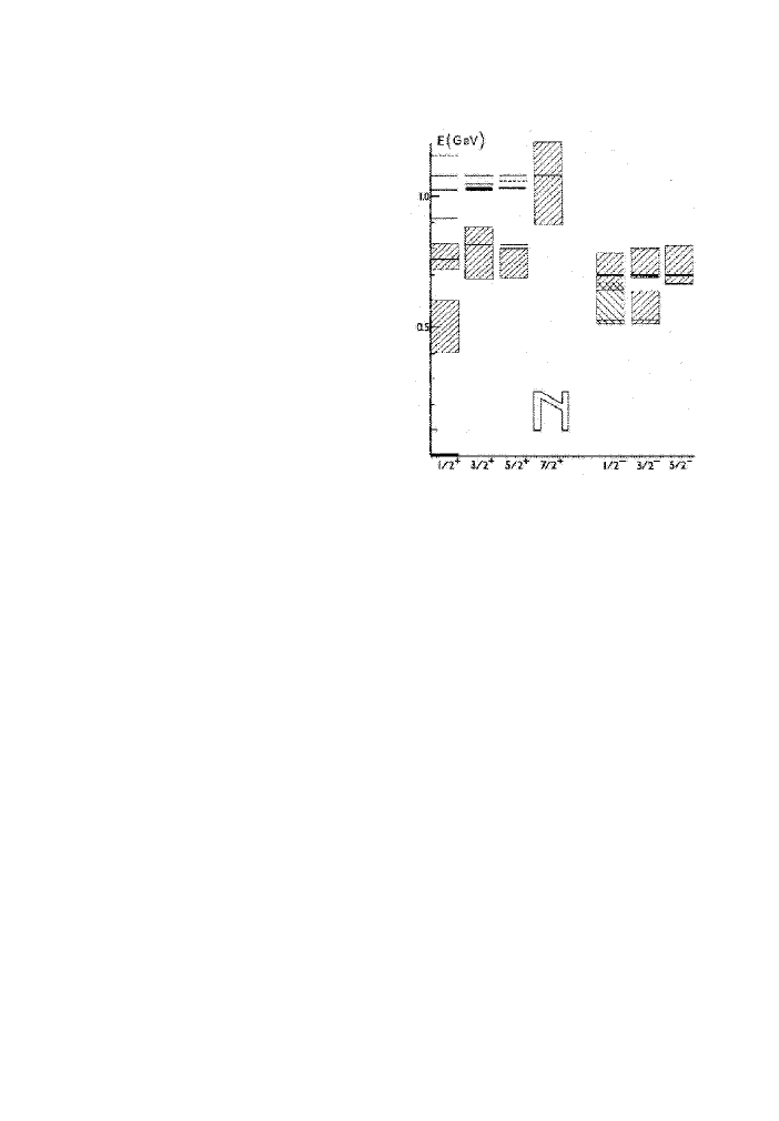
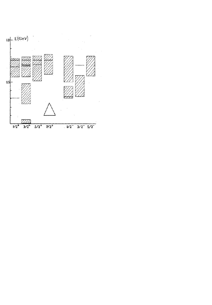
Figure 28: Relative energy N and $\Delta$ spectrum of reference [21].

6.2.3 Goldstone-boson exchange potential model

In this model the interaction between quarks is assumed to be given by a linear potential responsible for confinement plus a one-boson-exchange potential generated by the exchange of the octet of low-mass pseudoscalar mesons and a flavour singlet $\eta^{\prime}$ [45, 170], i.e.,

$$V=V_{\chi}+V_{conf}\,$$ (6.30)

where

$$\eqalign{V_{\chi}^{octet}(\vec{r_{ij}})&=\left[\sum_{a=1}^{3}V_{\pi}(\vec{r_{ij}})\lambda_{i}^{a}\lambda_{j}^{a}+\sum_{a=4}^{7}V_{K}(\vec{r_{ij}})\lambda_{i}^{a}\lambda_{j}^{a}+V_{\eta}(\vec{r_{ij}})\lambda_{i}^{8}\lambda_{j}^{8}\right]\vec{\sigma_{i}}\cdot\vec{\sigma_{j}}\\ V_{\chi}^{singlet}(\vec{r_{ij}})&={2\over 3}V_{\eta^{\prime}}\vec{\sigma_{i}}\cdot\vec{\sigma_{j}}}\,.$$ (6.31)

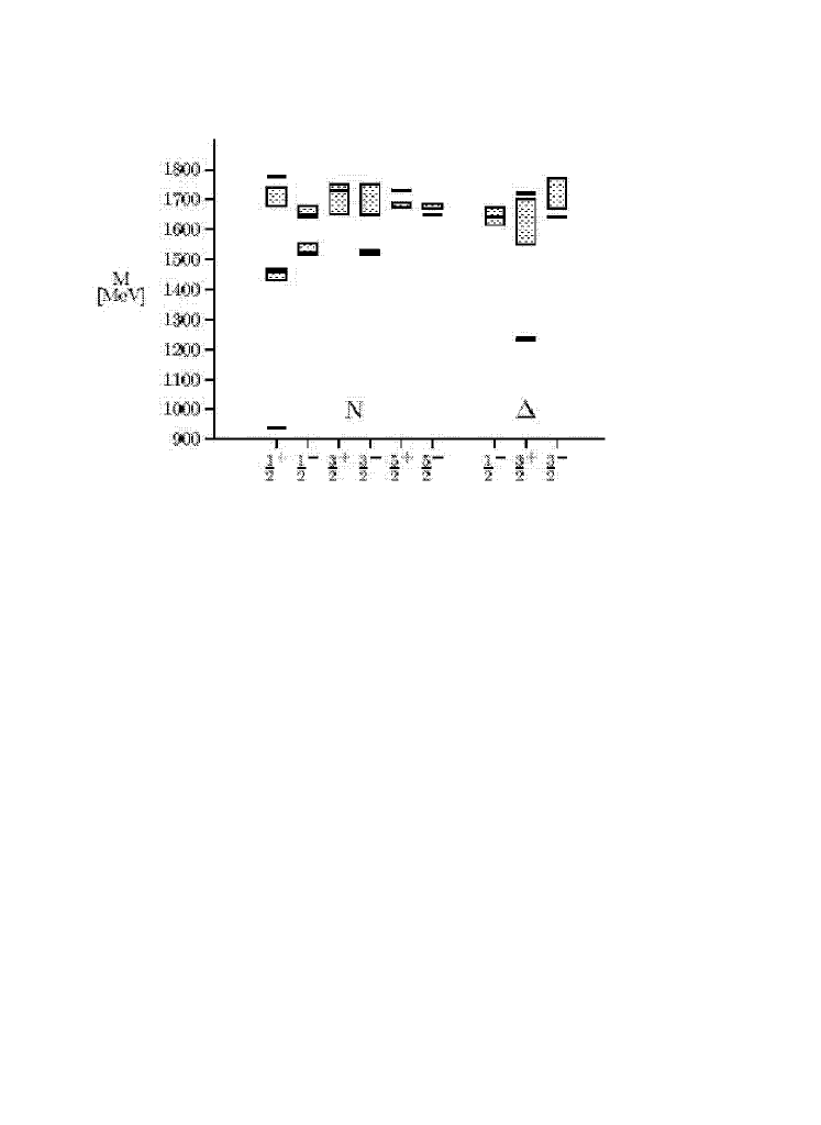
Figure 29: Relative energy N and $\Delta$ spectrum of reference [170].

The model was first applied by Glozman and Riska [45] within a first-order perturbation theory approach. In the more elaborated calculations of the model the one-boson-exchange potentials were constructed with different meson-quark-quark coupling constants for the octet and singlet and were regularized at the origin by smearing the $\delta$-function part with appropriate cut-off parameters which are different for each meson. As the coordinate-space Faddeev method allows to obtain a solution only in the case of a non-relativistic kinetic energy operator and the effect of replacing the non-relativistic kinetic energy operator (6.7) by the relativistic one, i.e.,

$$H_{0}\rightarrow\sum_{i=1}^{3}\left(\sqrt{m_{i}^{2}+q_{i}^{2}}-m_{i}\right)\,,$$ (6.32)

was estimated to be important for the level ordering problem, a calculation in the stochastic variational formalism was carried out (see figure 29 from [170]). The fit to the experimental spectrum was remarkable up to 900 MeV excitation energy. The first positive- and negative-parity nucleon states were correctly predicted though some caution should be in order to judge the $\Delta$ case. Actually the Roper of the $\Delta$ was predicted above the first negative-parity state though experimental error bars do not allow in this case to draw any definitive conclusion.

6.2.4 Chiral constituent quark models

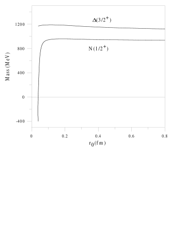
Figure 30: N$(1/2^{+})$ and $\Delta(3/2^{+})$ ground state masses as a function of $r_{0}$.

The non-strange baryon spectrum has been also studied from the chiral quark potential of section 2. Reference [44] presented a calculation with a small value for $r_{0}$ ($r_{0}=0.0367$ fm), the regularization parameter for the contact term of the OGE, and truncating the Hilbert space by means of a hyperspherical harmonic approach up to $k$ = 2 excitations. Similar results were presented in reference [171]. These results were strongly criticized [172] by arguing that such a small value of $r_{0}$ would give rise to unstable values for the baryon masses. Moreover, it was argued that the level ordering problem could not be solved with a chiral constituent quark model due to the presence of the OGE term and the subsequent reduction of the chiral quark coupling with respect to the Goldstone-boson exchange potential case. However the results of [44] and [171] can be alternatively reproduced almost exactly from a momentum-space Faddeev calculation including only the lowest order configurations $(\ell_{i},\lambda_{i},S_{i},T_{i})$ [173, 163] for a much bigger value of $r_{0}=$ 0.2 fm, lying in the stability region.

Table 8: Different sets of quark model parameters.

• Set	A	B	C	D
  $m_{q}({\rm MeV})$	313	313	313	313
  $\alpha_{s}$	0.72	0.65	0.485	0.50
  $a_{c}({\rm MeV}\cdot{\rm fm}^{-1})$	72.518	60.12	67.0	110.0
  $\alpha_{ch}$	0.0269	0.0269	0.0269	0.0269
  $r_{0}({\rm fm})$	0.2	0.8	0.25	0.74
  $m_{\sigma}({\rm fm}^{-1})$	3.42	3.42	3.42	3.42
  $m_{\pi}({\rm fm}^{-1})$	0.7	0.7	0.7	0.7
  $\Lambda_{\pi}({\rm fm}^{-1})$	4.2	5.4	4.2	2.0
  $\Lambda_{\sigma}({\rm fm}^{-1})$	4.2	4.2	4.2	2.0

The dependence of the N$(1/2^{+})$ and $\Delta(3/2^{+})$ ground state masses on the regularization parameter $r_{0}$, as given by the Faddeev calculation, is illustrated in figure 30. While the baryon-baryon interaction does not crucially depend on $r_{0}$, the baryon spectrum does. For values of $r_{0}$ below 0.1 fm the N$(1/2^{+})$ mass decreases very quickly while the $\Delta(3/2^{+})$ remains almost stable. As a consequence, the excitation energy of the whole spectrum would become too high. This result can be easily understood taken into account that the short-ranged spin-spin force is attractive for the nucleon but repulsive for the $\Delta$, lowering the $L=0$ nucleon states. It is also worth to notice that the nucleon ground state energy almost does not change for $r_{0}$ values greater than 0.1 fm.

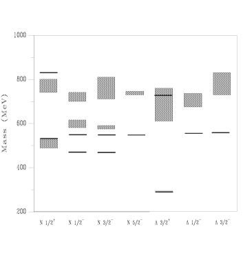
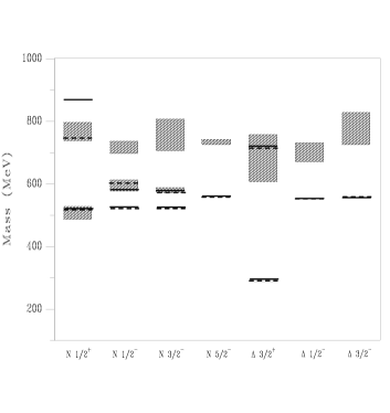
Figure 31: Relative energy N and $\Delta$ spectrum up to 1 GeV excitation energy for the set of parameters A (left) and B (right) of table 8.

Increasing the value of $r_{0}$ the excitation energy of all the states diminishes, but maintaining a similar ordering. The excitation energy can be easily increased just by changing the confinement strength and slightly modifying the strong coupling constant. The spectrum obtained in a lowest-order Faddeev calculation with the set of parameters A of table 8 is shown in figure 31, where the solid lines correspond to the predicted excitation energies with respect to the nucleon ground state and the shaded areas to the experimental values including their uncertainties. As can be seen, apart from the energy difference between the positive and negative parity excitations of the nucleon, the spectrum is almost the same as those reported in [44] and [171]. These results make clear that the regularization depends on the model space in which the calculation is done and the parameter of this regularization should not be understood as a true parameter of the model Hamiltonian but instead as a free parameter to be fitted.

Let us note that the level ordering problem remains in spite of the fact that the $(\vec{\sigma}_{i}\cdot\vec{\sigma}_{j})(\vec{\tau}_{i}\cdot\vec{\tau}_{j})$ structure of the pseudoscalar potential tends to favor the right location. Indeed, the correct ordering of the Roper and the negative parity excitations of the nucleon can be obtained by increasing the strength of the pseudoscalar potential. The strong correlation among the parameters of the model obliges for a modification of $\alpha_{s}$ and $a_{c}$ obtaining the set of parameters B of table 8. The spectrum obtained with this set of parameters is shown by solid lines in figure 31. It can be checked how the correct level ordering between the positive and negative parity can be obtained at the expense of having a stronger OPE (the dashed line in this figure stands for the results of reference [44]). However, enhancing artificially the pseudoscalar potential the agreement for the two-baryon sector, specially the binding energy of the deuteron, is destroyed [46]. Therefore in the lowest-order Faddeev calculation the level ordering problem has no solution if consistency with the two-baryon system is required.

Table 9: Convergence of baryon masses (in MeV) with respect to the number (Nr.) of configurations $(\ell_{i},\lambda_{i},S_{i},T_{i})$. See text for details.

• Nr.	$M_{\rm N}$	Nr.	$M_{\Delta}$	Nr.	$M_{{\rm N}^{*}(1440)}$	Nr.	$M_{{\rm N}^{*}(1535)}$
  2	115	1	423	2	641	4	643
  4	68	2	419	4	622	8	601
  6	21	3	418	6	587	12	570
  8	12			8	578	16	551
  10	2			10	562	20	540
  12	0			12	558

Let us now examine the situation when one extends the calculation to include all the configurations $(\ell_{i},\lambda_{i},S_{i},T_{i})$ with $\ell_{i}$ and $\lambda_{i}$ up to 5. The convergence with respect to the number of configurations is shown in table 9 for N, $\Delta$, N^∗(1440), and N^∗(1535) states corresponding to the set of parameters B of table 8 (figure 31). The mass difference with respect to the nucleon ground state mass as the reference (i.e., $M_{\rm N}=0$) is given. As can be seen, the convergence with respect to the number of configurations is different for different states. So, the $\Delta$ comes down by only 5 MeV while the N, N^∗(1440), and N^∗(1535) come down by approximately 100 MeV when one includes the higher orbital angular momentum configurations. It is also worth to notice that while in the lowest-order calculation the N^∗(1440) lies below the N^∗(1535), when one includes the higher orbital angular momenta the situation is reversed.

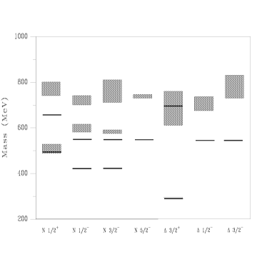
Figure 32: Relative energy N and $\Delta$ spectra up to 1 GeV excitation energy including all configurations with $\ell$ and $\lambda$ up to 5 for the set of parameters C.

Thus, the higher orbital angular momentum components play an important role on the description of the low-energy baryon spectrum. They influence the relative energy of the nucleonic and $\Delta$ sectors and they also affect the relative position of the positive- and negative-parity excitations of the nucleon. In figure 32 we show the baryon spectrum obtained with an extended Faddeev calculation for the set of parameters C of table 8 that correspond to the ones used for the description of the baryon-baryon interaction [43, 62]. The parameter $r_{0}$ has been taken as 0.25 fm, a typical value for spectroscopic models, such that the delta function of the OGE interaction is regularized in the stability region (see figure 30). As one can see, the relative position of the positive-parity states N, $\Delta$, and N^∗(1440) are correctly given, although the negative-parity states lie below the experimental results. It is interesting to check that the spectrum obtained is qualitatively very similar to the one obtained in [44]. The slope of the confining potential, $a_{c}$, which in set C of table 8 is 67.0 MeV fm^-1, is not so different from the value 72.5 MeV fm^-1 used in [44] .

It is worthwhile to investigate the role played by the OGE and OPE potentials in the level ordering problem. In reference [163] the energies of the N^∗(1440) and the N^∗(1535) were calculated starting with the set of parameters C and varying the contribution of the colour-magnetic interaction by modifying the coupling constant $\alpha_{s}$ of the OGE interaction. It turns out that the relative position of the N^∗(1440) and the N^∗(1535) is not very much affected by the modification of $\alpha_{s}$. This behaviour indicates that the correct level ordering between the negative and positive parity excited states of the nucleon does not come from a weakening of the OGE interaction. Furthermore, a suppression of the OGE would imply a stronger pseudoscalar interaction in order to reproduce the $\Delta-$N mass difference, and therefore one would obtain a model that it is incompatible with the understanding of the basic features of the two-nucleon system [46].

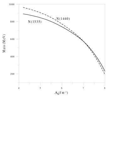
Figure 33: N^∗(1440) and N^∗(1535) masses as a function of the OPE cutoff mass.

Regarding the pseudoscalar interaction the $(\vec{\sigma}\cdot\vec{\sigma})(\vec{\tau}\cdot\vec{\tau})$ structure of the OPE gives attraction for symmetric spin-isospin pairs and repulsion for antisymmetric ones (a quite distinctive feature since the colour-magnetic part of the OGE gives similar contributions in both cases). This lowers the position of the first nucleon radial excitation, N^∗(1440), with regard to the first negative parity state solving part of the discrepancy between usual two-body potential models. To illustrate this point the energy of the N^∗(1440) and the N^∗(1535) was recalculated starting with the set of parameters C of table 8, but increasing the contribution of the pseudoscalar interaction by letting the OPE cutoff parameter $\Lambda_{\pi}$ to increase. The results are shown in figure 33. As can be seen, the inversion of the ordering between the positive and negative parity states can be achieved if $\Lambda_{\pi}$ becomes sufficiently large (around 7 fm^-1). A model with such a strong cutoff for the OPE is not realistic, the resulting $\Delta-$N mass difference being around 955 MeV. If one fits again the $\Delta-$N mass difference by modifying the confinement constant and suppressing the OGE one loses again the inversion between the negative and positive parity states.

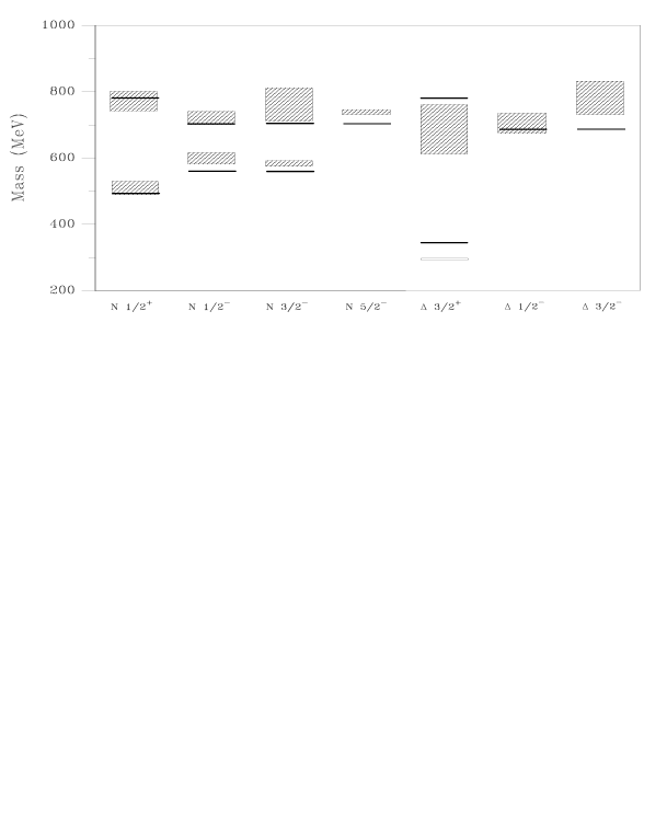
Figure 34: Relative energy N and $\Delta$ spectra up to 1 GeV excitation energy with relativistic kinematics for the set of parameters D of table 8.

Therefore we are forced to conclude that a consistent solution to the level ordering problem cannot be attained with the pure non-relativistic chiral constituent quark model.

Recently the baryon spectrum has been studied by means of a chiral constituent quark model incorporating relativistic kinematics [49]. We show in figure 34 the spectrum obtained from a momentum-space Faddeev calculation, in order to include full three-body relativistic kinematics using the set of parameters given in column D of table 8. As one sees the level-ordering problem that was evident in the spectrum of figure 32 has now been cured. As suggested long-time ago the relativistic kinematics has an important influence on the N^∗(1440) mass [174, 175] and the correct level ordering is obtained due to the combined effect of relativistic kinematics and one-pion-exchange. The OGE does not play a major role to this respect although it should be remarked that a decreasing of the strength of the OGE goes against the correct level ordering.

From a technical point of view, the replacement of the non-relativistic by the relativistic kinematics for short-range attractive interactions has to be done together with a careful study of the short-range part of the potential in the relativistic approach. This is due to the fact that the non-relativistic propagator falls down as $1/k^{2}$ while the relativistic one does as $1/k$. This is, for example, the reason why the semirelativistic solutions of reference [176] collapse when a scalar and an one-gluon-exchange potential are added to the pseudoscalar interaction. This makes evident the risk of replacing the non-relativistic kinetic energy by the relativistic one when the details of the short-range part of the potential are not well known.

6.2.5 Other potential models

In view of the importance of relativity with regard to the inversion of positive- and negative-parity nucleon states it is also interesting to mention studies using a fully covariant approach [177, 178, 179, 180]. This approach is based on the assumption of instantaneous interactions between the quarks which has the consequence that the three-quark Bethe-Salpeter equation reduces from its four-dimensional form to a three-dimensional form, the Salpeter equation, whose degree of complexity is similar to the non-relativistic Faddeev method.

A very complete study of the baryon spectrum has been carried out by the Bonn group [178, 179, 180] within a covariant formalism using the Salpeter equation and where the spin has been treated dynamically. Its model consists of a constant term, a linear confining term, and a residual quark-quark interaction. Two models of the part of the interaction containing the constant and confining terms (models A and B) which correspond to different choices for the Dirac structure of each of these terms are considered. The residual quark-quark interaction is based in ’t Hooft’s instanton-induced interaction. This determines its Dirac structure while its radial structure is taken of gaussian type $e^{-|\vec{r}_{ij}|^{2}/\lambda^{2}}$ with $\lambda=0.4$ fm. This instanton-induced interaction plays the role of the one-gluon-exchange potential in the more standard models. Since this interaction acts only in flavour-antisymmetric states it is responsible for the hyperfine splitting in the baryon spectrum. Thus, the $\Delta$ spectrum where all the states are flavour-symmetric is determined only by the constant and linear confining terms. This fact is used to fit the parameters of the two models (A and B). The strength of the instanton-induced residual interaction is then fitted to the $\Delta-$N mass splitting. A reasonable description of the $\Delta$ spectrum is obtained for both models. However, in the case of the nucleon spectrum only model A gives a satisfactory description, the problem of the inversion of positive- and negative-parity nucleon excitations being only partially cured since complete inversion is not achieved. This shows that relativity alone is not sufficient to give rise to the inversion of states observed in the experimental spectrum (as also demonstrated in reference [169]) being mandatory to this aim the inclusion of a pseudoscalar exchange interaction[49].

Let us finally mention that in reference [181] the mass spectrum of the low-lying ground-state baryons has been calculated by solving the Dirac equation for each quark in a single-particle confining potential and treating the residual interactions (OGE and OPE potentials) as low-order perturbations.

6.2.6 Consistency of the baryon spectrum wave functions with the ansatz baryon-baryon wave functions

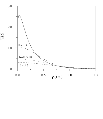
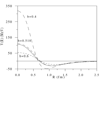
Figure 35: Main hyperradial component of the nucleon wave function $\Psi(\rho)$ and diagonal kernels of the NN potential $V(R)$ for the $(S,T)=(1,0)$ channel. The solid line corresponds to the solution of the Schödinger equation, the long, medium and short-dashed lines to gaussian ansatz with values of the parameter $b=$ 0.4, 0.518, and 0.6 fm, respectively.

After discussing the one-baryon problem one question should immediately arise. The two-baryon system has been studied by means of gaussian-like wave functions for the spatial part while later on the one-baryon problem has been solved and therefore one has the baryon wave functions predicted by the quark-quark Hamiltonian. Does it make sense the gaussian hypothesis for the radial part of the wave function? To answer this question figure 35 compares the wave function predicted by the quark-quark Hamiltonian used for figure 32 to the ansatz used to study the baryon-baryon interaction for three different values of the oscillator parameter. Although at long range all the wave functions look very similar, the discrepancy at the origin may reach a factor four. This effect may be very important for quantities depending on the value of the wave function at small distances. Hence an evaluation of the importance of this difference in the calculation of the phase shifts should be done. From the technical point of view a complete RGM calculation would be very difficult to perform with the full solution of the Schrödinger equation, but one can easily compare the diagonal kernels of the NN potential (which correspond to the diagonal part used to calculate the phase shifts and the deuteron properties) with both type of wave functions as shown in figure 35. We see how the NN potential calculated with the full solution of the Schrödinger equation looks pretty similar to the potential calculated with the harmonic oscillator wave function with $b=$0.518 fm, this is precisely the value used in the RGM calculation of the phase shifts and deuteron properties conferring to it a self-consistent character. Other values of $b$ give quite different potentials even in the medium-long range part. In this way the validity of the gaussian ansatz wave function in the RGM calculations is confirmed, and the old controversy about the possible values of the parameter $b$ can be solved.

6.3 Exotic baryons

Once the baryon spectrum has been analyzed one may wonder about the predictions of chiral quark models for exotic baryons, i.e., systems with baryon number $+1$ whose quantum numbers cannot correspond to a simple three-quark picture. There has been a renewed interest on this subject from the announcement of the discovery of the so-called $\Theta^{+}$ resonance, with strangeness $+1$, in several experiments listed in Table 10. This resonance, carrying unit positive charge, shows out as a peak in the invariant mass distribution of $(K^{+}n)$ or $(K_{S}^{0}p)$. The location of the peak corresponds to an invariant mass that ranges from 1520 to 1570 MeV depending on the experiment and a small width in all cases lesser than 25 MeV (actually $K$N phase shifts analyses give an upper bound of $\sim$ 1 MeV, see reference [208] and references therein). The angular momentum and parity of the resonance are still experimentally undetermined whereas there are experimental indications on its iso-singlet character [186]. After the initial excitement several recent experiments also listed in Table 10 have failed to find evidence for pentaquark signals (see Ref. [209] for a detailed description of the experiments).

Different possible explanations for such a peak have been discussed. Leaving aside its possible origin as a kinematic reflection of the intermediate production of known meson resonances [210] what deserves a complete analysis and having been discarded its $K$N scattering potential nature, the most compelling explanations are associated to a chiral soliton or a pentaquark $(udud\overline{s})$ structure. The chiral soliton model by Diakonov, Petrov and Polyakov [10] predicts an exotic $1/2^{+}$ baryon belonging to the $\overline{10}_{F}$ representation of $SU(3)_{Flavour}$ with a mass around 1540 MeV and a width less than 15 MeV (this number has been recalculated as 30 MeV in reference [211]) stimulated its experimental search. It should be also mentioned that years before Praszalowicz [212] predicted with a Skyrme model a 1530 MeV mass for the iso-singlet member of the antidecuplet.

From a quark model point of view and under the assumption of a $J^{P}=1/2^{+}$ assignment, alternative mechanisms, mainly based on colour or chiral interactions, have been proposed.

Table 10: Overview of the positive and null pentaquark experiments.

Positive experiments
Exp.	Reaction	Mass (MeV/c2)	Width (MeV)	Significance	Ref.
LEPS(1)	$\gamma^{12}C\to K^{+}K^{-}X$	1540$\pm$10	$<25$	4.6$\sigma$	[182]
LEPS(2)	$\gamma d\to K^{+}K^{-}X$	$\sim 1540$	$-$	$-$	[183]
DIANA	$K^{+}Xe\to K^{0}_{s}p(Xe)^{\prime}$	1539$\pm$2	$<9$	4.4$\sigma$	[184]
CLAS-d	$\gamma d\to K^{+}K^{-}p(n)$	1542$\pm$5	$<21$	5.2$\sigma$	[185]
SAPHIR	$\gamma p\to K^{+}K^{0}_{S}(n)$	1540$\pm$6	$<25$	4.8$\sigma$	[186]
CLAS-p	$\gamma p\to K^{+}K^{-}\pi^{+}(n)$	1555$\pm$10	$<26$	7.8$\sigma$	[187]
ITEP	$\nu A\to K^{0}_{S}pX$	1533$\pm$5	$<20$	6.7$\sigma$	[188]
SVD	$pA\to pK^{0}_{S}X$	1526$\pm$3	$<24$	5.6$\sigma$	[189]
HERMES	$e^{+}d\to K^{0}_{S}pX$	1526$\pm$3	13$\pm$9	$\sim 5\sigma$	[190]
ZEUS	$ep\to K^{0}_{S}pX$	1522$\pm$3	8$\pm$4	$\sim 5\sigma$	[191]
COSY	$pp\to K^{0}_{S}p\Sigma^{+}$	1530$\pm$5	$<18$	$\sim 5\sigma$	[192]
Null experiments
Exp.		Reaction			Ref.
HERA-B		$pA\to\Theta^{+}X$			[193]
BES		$e^{+}e^{-}\to J/\psi[\psi(2S)]\to\Theta\overline{\Theta}$			[194]
CDF		$p\overline{p}\to\Theta^{+}X$			[195]
BaBar		$e^{+}e^{-}\to\Upsilon(4S)$			[196]
ALEPH		$e^{+}e^{-}\to Z\to q\overline{q}$			[197]
DELPHI		$e^{+}e^{-}\to Z\to q\overline{q}$			[198]
FNAL E690		$pp\to pK^{-}\pi^{+}\Theta^{+}$			[199]
HyperCP		($\pi^{+},K^{+},p)Cu\to\Theta^{+}X$			[200]
PHENIX		$dAu\to\Theta^{+}X$			[201]
BELLE		$KN\to\Theta^{+}X$			[202]
FOCUS		$\gamma p\to\Theta^{+}X$			[203]
LASS		$K^{+}p\to K^{+}n\pi^{+}$			[204]
L3		$\gamma\gamma\to\Theta\overline{\Theta}$			[205]
SELEX		$(\pi,p,\Sigma)p\to\Theta^{+}X$			[206]
SPHINX		$pC(N)\to\Theta^{+}\overline{K^{0}}C(N)$			[207]

Among the colour based models we shall mention the diquark-diquark and diquark-triquark models. One should first realize that a simple independent quark model based on a confinement plus OGE potential would predict the ground state pentaquark to have negative parity, since the four quarks and the antiquark would be in $0s$ states and the intrinsic parity of the antiquark is negative. This difficulty can be overcome by introducing multiquark correlations. Jaffe and Wilczek [213], realizing the presence of strong colour-spin correlations in the baryon spectrum, built a diquark-diquark-antiquark $((ud)(ud)\overline{s}$) model with the diquark structures $(3_{Flavour},3_{Colour},S=0)$ favoured by the colour magnetic (spin-spin) OGE interaction. The assignment of the nucleon Roper resonance as well as the $\Theta$ to the same $\overline{10}_{F}$ representation allowed for an understanding not only of the pentaquark mass but also of the Roper mass on the basis of three-quark $8_{F}-$pentaquark $\overline{10}_{F}$ mixing. On the other hand Karliner and Lipkin [214] proposed a diquark-triquark model $((ud)(ud\overline{s}))$ with a triquark $(\overline{6}_{F},3_{C},S=1/2)$ structure so that the diquark and triquark have a colour electric OGE interaction (the Coulomb term) between them which is identical to the quark-antiquark interaction in a meson. Both models give the right mass for the pentaquark. The small width is attributed to the weak coupling to the $KN$ continuum due to the difference in colour, spin and spatial wave functions. Both models predict new stable pentaquarks in the heavy quark sectors what could serve, if experimentally found, to disentangle the role of quark correlations.

On the other hand chiral quark models may provide a natural explanation for the positive parity ground state pentaquark. This is not surprising since they incorporate Goldstone bosons merging from spontaneous chiral symmetry breaking and it is precisely this breaking the crucial fact in the formulation of the chiral soliton model. Explicitly the flavour-spin interaction may shift the orbitally excited four-quark state below the $(0s)^{4}$ since the $L=1$ configuration allows for a completely symmetric flavour-spin four quark wave function whereas the $(0s)^{4}$ configuration does not [215]. This parity inversion is similar to the one giving rise to the correct level ordering in the nucleon spectrum as we have seen. Stancu and Riska [216] have pointed out that pentaquark stability could be provided by a strong spin-spin interaction between the light flavour and the strange antiquark.

These arguments should encourage more work along these lines in order to get a deeper understanding at the theoretical level. From the experimental point of view further experiments are needed to clarify the situation.

7 Dibaryons and tribaryons

The possible existence of unstable non-strange two- and three-baryon resonances corresponding to bound-state solutions of systems composed of nucleons and deltas has been speculated for years [217, 218, 219, 220, 221, 222, 223, 224, 225, 226]. In the case of two-body systems (that we shall refer to as dibaryons) they will decay mainly into two nucleons and either one or two pions, while for the three-body case (tribaryons) they will decay mainly into three nucleons and either one, two, or three pions. In principle, any nucleus with at least three nucleons can serve as test system that may be excited by forming a dibaryon or a tribaryon [227]. The lifetime of bound states involving one or more $\Delta$’s should be similar to that of the $\Delta$ in the case of very weakly bound systems and larger if the system is very strongly bound. Therefore, these resonances will have widths similar or smaller than the width of the $\Delta$ so that, in principle, they may be experimentally observable.

7.1 Dibaryons in the constituent quark model

The study of dibaryon resonances within the framework of the constituent quark model has generally been carried out by considering the baryon-baryon interaction obtained from a model consisting of confinement and a OGE interaction. This baryon-baryon interaction exhibits a repulsive core at short distances in most channels due to quark antisymmetrization effects and the hyperfine quark-quark interaction. Thus, dibaryons may exist in such channels where the strong short-range repulsion is missing and therefore quark-exchange forces can produce a tight deep bound state of six quarks.

The detailed investigation of the nature (attractive or repulsive) of the different channels of the NN, N$\Delta$, and $\Delta\Delta$ systems has been an important subject of study ever since the first applications of the constituent quark model to derive a baryon-baryon interaction. Oka and Yazaki [30] showed that the Pauli principle and the OGE interaction generate a hard core in the NN $(j,i)$ ($j$ stands for the total angular momentum and $i$ for the isospin) channels (0,1) and (1,0), whereas in the $\Delta\Delta$ channels (0,3) and (3,0) the interaction is strongly attractive such that the $(j,i)=(3,0)$ channel is bound. In a later revised analysis by Oka [95] the $\Delta\Delta$ $(j,i)$ channels (1,0), (0,1), and (3,0) were found to be attractive while the channel (0,3) was weakly repulsive.

The $\Delta\Delta$ states $(j,i)=(0,3)$ and (3,0) have also been studied by Maltman [218] using the standard confinement and OGE interaction model constructed in [228]. He found that the (3,0) state is bound by 260 MeV while the (0,3) state is bound by only 30 MeV which is in qualitative agreement with the results of Oka and Yazaki [30, 95] and Cvetič et al[98].

The $\Delta\Delta$ state $(j,i)=(3,0)$ has been called the deltaron by Goldman and collaborators [97, 96] since this state is the analogue of the deuteron in the case of two $\Delta^{\prime}s$. Their model incorporates the OGE interaction as well as the quark delocalization (similar to electron delocalization in nuclear physics) and color screening (predicted by unquenched lattice calculations). Indeed the combined effect of the last two terms produces the intermediate-range attraction observed in the NN system. The binding energy of the (3,0) state in their model is larger than 200 MeV so that the state lies below the $\pi{\rm N}\Delta$ threshold.

7.2 Dibaryons and tribaryons in the chiral constituent quark model

This study of the possible existence of such structures has been done with the help of the baryon-baryon interactions obtained from the chiral constituent quark model described in section 2. It presents the advantage that once the model parameters are fixed in the study of the NN system, all the other interacting potentials are parameter-free. Besides, it allows for a comparison of the results obtained by means of the local (BO potential) and non-local (RGM potential) interactions derived from the underlying quark-quark potential.

In order to perform the calculations one can assume that the $\Delta$ is a stable particle, that is, one can neglect its width and the effects of retardation in the OPE interaction of the baryon-$\Delta$ subsystems. These two effects have been estimated in the case of the simple N$\Delta$ system [229]. There, it was found that the assumption of a stable $\Delta$ leads to very reliable predictions for the mass of N$\Delta$ resonances since the effects of retardation and width of the $\Delta$ are responsible for producing the width of the N$\Delta$ resonance but have almost no effect over its mass. Thus, one can be confident that the masses of the bound states containing $\Delta$’s will not change very much when its unstable nature is explicitly taken into account. For the three-baryon systems one can take advantage of the experience gained in the three-nucleon bound-state problem [230, 231], where one knows that the dominant configuration is that in which all particles are in $S$-wave states. However, in order to get reasonable results for the binding energy, the $S$-wave two-body amplitudes used as input in the Faddeev equations must also contain the effect of the tensor force. So, for example, in the case of the Reid soft-core potential if one considers only the $S$-wave configurations but neglects the tensor force in the two-body subsystems there is no bound triton. However, including the effect of the tensor force in the NN ${}^{3}S_{1}-{}^{3}\!D_{1}$ channel, but using only the ${}^{1}S_{0}$ and ${}^{3}S_{1}$ components of the two-body amplitudes in the three-body equations (2-channel calculation), one gets a triton binding energy of 6.58 MeV against the experimental value 8.49 MeV. Notice that including the remaining configurations (34-channel calculation) a triton binding energy of 7.35 MeV is obtained [232]. This means that the $S$-wave truncated T-matrix approximation leads to a binding energy which differs from the exact value by less than 1 MeV. Hence this approach may be efficient to look for the best candidates for bound states and the energy ordering of the different tribaryon systems.

7.2.1 Formalism of two-body bound states

Let us consider two baryons $B_{1}$ and $B_{2}$ in a relative $S$-wave interacting through a potential that contains a tensor force. Then there is a coupling to the $B_{1}B_{2}$ $D$-wave so that the Lippmann-Schwinger equation of the system is of the form

$$t_{i;j_{i}i_{i}}^{l_{i}s_{i}l_{i}^{\prime\prime}s_{i}^{\prime\prime}}(p_{i},p_{i}^{\prime\prime};E)=V_{i;j_{i}i_{i}}^{l_{i}s_{i}l_{i}^{\prime\prime}s_{i}^{\prime\prime}}(p_{i},p_{i}^{\prime\prime})+\sum_{l_{i}^{\prime}s_{i}^{\prime}}\int_{0}^{\infty}{p_{i}^{\prime}}^{2}dp_{i}^{\prime}\,V_{i;j_{i}i_{i}}^{l_{i}s_{i}l_{i}^{\prime}s_{i}^{\prime}}(p_{i},p_{i}^{\prime})$$

$$\times{1\over E-{p_{i}^{\prime}}^{2}/2\eta_{i}+i\epsilon}t_{i;j_{i}i_{i}}^{l_{i}^{\prime}s_{i}^{\prime}l_{i}^{\prime\prime}s_{i}^{\prime\prime}}(p_{i}^{\prime},p_{i}^{\prime\prime};E),$$ (7.1)

where $j_{i}$ and $i_{i}$ are the total angular momentum and isospin of the system, while $l_{i}s_{i}$, $l_{i}^{\prime}s_{i}^{\prime}$, and $l_{i}^{\prime\prime}s_{i}^{\prime\prime}$ are the initial, intermediate, and final orbital angular momentum and spin of the system, respectively. $p_{i}$ and $\eta_{i}$ are, respectively, the relative momentum and reduced mass of the two-body system. Tables 11 and 12 show the corresponding NN, N$\Delta$ and $\Delta\Delta$ two-body channels in a relative $S$-wave that are coupled together for the possible values of $j$ and $i$ (since the NN state is the one with the lowest mass, in this case we have considered also the possibility of transitions to larger mass states like N$\Delta$ and $\Delta\Delta$). In the NN and $\Delta\Delta$ cases the Pauli principle requires $(-)^{l_{i}+s_{i}+i_{i}}=-1$.

Table 11: NN channels $(l_{\rm NN},s_{\rm NN})$, N$\Delta$ channels $(l_{{\rm N}\Delta},s_{{\rm N}\Delta})$, and $\Delta\Delta$ channels $(l_{\Delta\Delta},s_{\Delta\Delta})$ that are coupled together in the ${}^{3}S_{1}-{}^{3}\!D_{1}$ and ${}^{1}S_{0}$ NN states.

• NN state	$j$	$i$	$(l_{\rm NN},s_{\rm NN})$	$(l_{{\rm N}\Delta},s_{{\rm N}\Delta})$	$(l_{\Delta\Delta},s_{\Delta\Delta})$
  ${}^{3}S_{1}-{}^{3}\!D_{1}$	1	0	(0,1),(2,1)	$-$	(0,1),(2,1),(2,3)
  ${}^{1}S_{0}$	0	1	(0,0)	(2,2)	$-$

Table 12: Coupled channels $(l,s)$ that contribute to a given N$\Delta$ or $\Delta\Delta$ state with total angular momentum $j$ and isospin $i$.

• 		N$\Delta$	$\Delta\Delta$
  $j$	$i$	$(l,s)$	$(l,s)$
  0	1	$-$	(0,0),(2,2)
  1	0	$-$	(0,1),(2,1),(2,3)
  1	1	(0,1),(2,1),(2,2)	$-$
  1	2	(0,1),(2,1),(2,2)	(0,1),(2,1),(2,3)
  2	1	(0,2),(2,1),(2,2)	(0,2),(2,0),(2,2)
  2	2	(0,2),(2,1),(2,2)	$-$
  0	3	$-$	(0,0),(2,2)
  3	0	$-$	(0,3),(2,1),(2,3)
  2	3	$-$	(0,2),(2,0),(2,2)
  3	2	$-$	(0,3),(2,1),(2,3)

As mentioned before, for the solution of the three-body system one can use only the component of the T-matrix obtained from the equation (7.1) with $l_{i}=l_{i}^{\prime\prime}=0$, so that for that purpose one can define the $S$-wave truncated amplitude

$$t_{i;s_{i}i_{i}}(p_{i},p_{i}^{\prime\prime};E)\equiv t_{i;s_{i}i_{i}}^{0s_{i}0s_{i}}(p_{i},p_{i}^{\prime\prime};E).$$ (7.2)

7.2.2 Formalism of three-body bound states

Table 13: Two-body $\Delta\Delta$ (NN) channels $(j,i)$ that contribute to a given $\Delta\Delta\Delta$ (NNN) state with total spin $S$ and isospin $I$.

• 		NN	$\Delta\Delta$
  $S$	$I$	$(j,i)$	$(j,i)$
  1/2	1/2	(1,0),(0,1)	(1,2),(2,1)
  1/2	3/2	(0,1)	(1,0),(1,2),(2,1),(2,3)
  3/2	1/2	(1,0)	(0,1),(1,2),(2,1),(3,2)
  1/2	5/2	$-$	(1,2),(2,1),(2,3)
  5/2	1/2	$-$	(1,2),(2,1),(3,2)
  1/2	7/2	$-$	(1,2),(2,3)
  7/2	1/2	$-$	(2,1),(3,2)
  1/2	9/2	$-$	(2,3)
  9/2	1/2	$-$	(3,2)
  3/2	3/2	$-$	(0,1),(0,3),(1,0),(1,2), (2,1),(2,3),(3,0),(3,2)
  3/2	5/2	$-$	(0,1),(0,3),(1,2),(2,1), (2,3),(3,2)
  5/2	3/2	$-$	(1,0),(1,2),(2,1),(2,3), (3,0),(3,2)
  3/2	7/2	$-$	(0,3),(1,2),(2,3),(3,2)
  7/2	3/2	$-$	(2,1),(2,3),(3,0),(3,2)
  3/2	9/2	$-$	(0,3),(2,3)
  9/2	3/2	$-$	(3,0),(3,2)
  5/2	5/2	$-$	(1,2),(2,1),(2,3),(3,2)
  5/2	7/2	$-$	(1,2),(2,3),(3,2)
  7/2	5/2	$-$	(2,1),(2,3),(3,2)
  5/2	9/2	$-$	(2,3)
  9/2	5/2	$-$	(3,2)
  7/2	7/2	$-$	(2,3),(3,2)
  7/2	9/2	$-$	(2,3)
  9/2	7/2	$-$	(3,2)
  9/2	9/2	$-$	$-$

If one restricts to configurations where all three particles are in $S$-wave states, the Faddeev equations for the bound-state problem in the case of three particles with total spin $S$ and isospin $I$ are (see equation (6.18))

$$T_{i;SI}^{s_{i}i_{i}}(p_{i}q_{i})=\sum_{j\neq i}\sum_{s_{j}i_{j}}<s_{i}i_{i}|s_{j}i_{j}>_{SI}{1\over 2}\int_{0}^{\infty}q_{j}^{2}dq_{j}\int_{-1}^{1}dcos\theta\,t_{i;s_{i}i_{i}}(p_{i},p^{\prime}_{i};E-q_{i}^{2}/2\nu_{i})$$

$$\times{1\over E-p_{j}^{2}/2\eta_{j}-q_{j}^{2}/2\nu_{j}}\,T_{j;SI}^{s_{j}i_{j}}(p_{j}q_{j}),$$ (7.3)

where $p_{i}$ and $q_{i}$ are the usual momentum-space Jacobi coordinates (see section 6.1.5), $\eta_{i}$ and $\nu_{i}$ are the reduced masses defined by equations (6.19) and (6.20), and $<s_{i}i_{i}|s_{j}i_{j}>_{SI}$ are the spin-isospin coefficients given by equation (6.21).

Table 14: Two-body N$\Delta$ $(j_{{\rm N}\Delta},i_{{\rm N}\Delta})$ and NN channels $(j_{\rm NN},i_{\rm NN})$ that contribute to a given NN$\Delta$ state with total spin $S$ and isospin $I$.

• $S$	$I$	$(j_{{\rm N}\Delta},i_{{\rm N}\Delta})$	$(j_{\rm NN},i_{\rm NN})$
  1/2	1/2	(1,1)
  1/2	3/2	(1,1),(1,2)	(1,0)
  1/2	5/2	(1,2)
  3/2	1/2	(1,1),(2,1)	(0,1)
  3/2	3/2	(1,1),(1,2),(2,1),(2,2)	(1,0),(0,1)
  3/2	5/2	(1,2),(2,2)	(0,1)
  5/2	1/2	(2,1)
  5/2	3/2	(2,1),(2,2)	(1,0)
  5/2	5/2	(2,2)

Table 15: Two-body N$\Delta$ $(j_{{\rm N}\Delta},i_{{\rm N}\Delta})$ and $\Delta\Delta$ channels $(j_{\Delta\Delta},i_{\Delta\Delta})$ that contribute to a given N$\Delta\Delta$ state with total spin $S$ and isospin $I$.

• $S$	$I$	$(j_{{\rm N}\Delta},i_{{\rm N}\Delta})$	$(j_{\Delta\Delta},i_{\Delta\Delta})$
  1/2	1/2	(1,1),(1,2),(2,1),(2,2)	(1,0),(0,1)
  1/2	3/2	(1,1),(1,2),(2,1),(2,2)	(0,1),(1,2)
  1/2	5/2	(1,1),(1,2),(2,1),(2,2)	(0,3),(1,2)
  1/2	7/2	(1,2),(2,2)	(0,3)
  3/2	1/2	(1,1),(1,2),(2,1),(2,2)	(1,0),(2,1)
  3/2	3/2	(1,1),(1,2),(2,1),(2,2)	(1,2),(2,1)
  3/2	5/2	(1,1),(1,2),(2,1),(2,2)	(1,2),(2,3)
  3/2	7/2	(1,2),(2,2)	(2,3)
  5/2	1/2	(1,1),(1,2),(2,1),(2,2)	(2,1),(3,0)
  5/2	3/2	(1,1),(1,2),(2,1),(2,2)	(2,1),(3,2)
  5/2	5/2	(1,1),(1,2),(2,1),(2,2)	(2,3),(3,2)
  5/2	7/2	(1,2),(2,2)	(2,3)
  7/2	1/2	(2,1),(2,2)	(3,0)
  7/2	3/2	(2,1),(2,2)	(3,2)
  7/2	5/2	(2,1),(2,2)	(3,2)
  7/2	7/2	(2,2)

The three amplitudes $T_{1;SI}^{s_{1}i_{1}}(p_{1}q_{1})$, $T_{2;SI}^{s_{2}i_{2}}(p_{2}q_{2})$, and $T_{3;SI}^{s_{3}i_{3}}(p_{3}q_{3})$ in equation (7.3) are coupled together. The number of coupled equations can be reduced since some of the particles are identical. In the case of three identical particles (NNN and $\Delta\Delta\Delta$ systems) all three amplitudes are equal and therefore equation (7.3) becomes,

$$T_{i;SI}^{s_{i}i_{i}}(p_{i}q_{i})=\sum_{s_{j}i_{j}}<s_{i}i_{i}|s_{j}i_{j}>_{SI}\int_{0}^{\infty}q_{j}^{2}dq_{j}\int_{-1}^{1}dcos\theta\,t_{i;s_{i}i_{i}}(p_{i},p^{\prime}_{i};E-q_{i}^{2}/2\nu_{i})$$

$$\times{1\over E-p_{j}^{2}/2\eta_{j}-q_{j}^{2}/2\nu_{j}}\,T_{j;SI}^{s_{j}i_{j}}(p_{j}q_{j}).$$ (7.4)

Table 13 details the three NNN states characterized by total spin and isospin $(S,I)$ that are possible as well as the two-body NN channels that contribute to each state. The 25 possible $\Delta\Delta\Delta$ states as well as the two-body $\Delta\Delta$ channels that contribute to each state are also given.

When two particles are identical and one different (NN$\Delta$ and N$\Delta\Delta$ systems) two of the amplitudes are equal. With the assumption that particle 1 is the different one and particles 2 and 3 are the two identical, only the amplitudes $T_{1;SI}^{s_{1}i_{1}}(p_{1}q_{1})$ and $T_{2;SI}^{s_{2}i_{2}}(p_{2}q_{2})$ are independent from each other. The reduction procedure for the case where one has two identical fermions has been described in [156] and [233] and will not be repeated here. Tables 14 and 15 resume the possible NN$\Delta$ and N$\Delta\Delta$ states characterized by its total spin and isospin $(S,I)$ as well as the two-body N$\Delta$ and NN, or N$\Delta$ and $\Delta\Delta$, channels that contribute to each state.

7.2.3 Results

Before going to the numbers obtained two technical precisions are in order. It has been already discussed in section 3.1 that the $(j,i)=$ (1,1) and (2,2) N$\Delta$ states, and the $(j,i)=$ (2,3) and (3,2) $\Delta\Delta$ states present quark Pauli blocking for $L=0$, what translates into a strong repulsive core in the baryon-baryon potential. The reason for such a repulsive core is the presence of a forbidden state, that in the RGM potential should be eliminated from the relative motion wave function for each partial wave. This procedure is tedious both from the conceptual and numerical point of view [70, 234]. It has been demonstrated [27] that for the Pauli blocked channels the local N$\Delta$ and $\Delta\Delta$ potentials reproduce the qualitative behaviour of the RGM kernels after the subtraction of the forbidden states. This is why reference [225] used the local version of the quark Pauli blocked channels.

For the three-body systems the binding-energy spectrum, say, the energy of the states measured with respect to the three-body threshold, as well as the separation-energy spectrum, the energy of the states measured with respect to the threshold of one-free particle and a bound state of the other two, will be calculated. The deepest bound three-body state is not the one with the largest binding energy but the one with the largest separation energy, since such a state is the one that requires more energy in order to become unbound, that is, to move it to the nearest threshold. The numerical results for two-body and three-body systems appear in tables 16 and 17 respectively.

7.2.4 The NN system

Out of the two states of table 11 only the $(j,i)=(1,0)$, that is the deuteron, is bound. The non-local model gives a deuteron binding energy of 2.14 MeV, while the local version gives 3.13 MeV. The exact chiral constituent quark model NN potential gives a deuteron binding energy of 2.225 MeV [135]. This value was obtained by taking into account the $\Delta\Delta$ partial wave $(l_{\Delta\Delta},s_{\Delta\Delta})=(4,3)$ coupled together in addition to those given in table 11. The present calculation only considers $S$- and $D$-waves obtaining for the non-local potential a deuteron binding energy of 2.14 MeV, which differs less than 0.1 MeV from the exact result.

7.2.5 The N$\Delta$ system

Out of the four possible N$\Delta$ states of table 12 only one, the $(j,i)=(2,1)$, has a bound state which lies exactly at the N$\Delta$ threshold for the local model, and with a small binding of 0.141 MeV for the non-local one. The states $(j,i)=(1,1)$ and $(2,2)$ are unbound because they present quark Pauli blocking that, as in the case of the $\Delta\Delta$ system, will play an important role in the three-body spectrum. The state $(j,i)=(2,1)$ can also exist in the NN system and there it corresponds to the ${}^{1}D_{2}$ partial wave which has a resonance at an invariant mass of 2.17 GeV [235, 237, 236]. This means that the N$\Delta$ bound state may decay into two nucleons and appear in the NN system as a resonance. As the N$\Delta$ bound state has for both local and non-local models energies very close to the N$\Delta$ threshold, the invariant mass of the system should be very close to 2.17 GeV. Thus, the chiral constituent quark model predicts the NN ${}^{1}D_{2}$ resonance as being a N$\Delta$ bound state.

7.2.6 The $\Delta\Delta$ system

Out of the eight possible $\Delta\Delta$ states given in table 12 with the non-local interaction five have a bound state, whereas the local interaction binds six of them (in both cases there are no excited states in any channel). The channels $(j,i)=(2,3)$ and $(3,2)$ are unbound as expected, due to the strong repulsive barrier at short distances in the $S$-wave central interaction. These repulsive cores will largely determine the three-body spectrum.

Table 16: Binding energies $B_{2}$ (in MeV) of the NN, N$\Delta$ and $\Delta\Delta$ states. ’ub’ denotes unbound channels. $B_{2}^{L}$ ($B_{2}^{NL}$) refers to the local (nonlocal) potential.

• 		NN		N$\Delta$		$\Delta\Delta$
  $j$	$i$	$B_{2}^{L}$	$B_{2}^{NL}$	$B_{2}^{L}$	$B_{2}^{NL}$	$B_{2}^{L}$	$B_{2}^{NL}$
  0	1	ub	ub	$-$	$-$	108.4	159.5
  1	0	3.13	2.14	$-$	$-$	138.5	190.3
  1	1	$-$	$-$	ub	ub	$-$	$-$
  1	2	$-$	$-$	ub	ub	5.7	ub
  2	1	$-$	$-$	0.0	0.141	30.5	7.4
  2	2	$-$	$-$	ub	ub	$-$	$-$
  0	3	$-$	$-$	$-$	$-$	0.4	0.2
  3	0	$-$	$-$	$-$	$-$	29.9	7.8
  2	3	$-$	$-$	$-$	$-$	ub	ub
  3	2	$-$	$-$	$-$	$-$	ub	ub

The predicted bound states $(j,i)$ = (1,0), (0,1), (2,1) and (3,0) appear also in the NN system. One can see that the deepest bound state is $(j,i)$ = (1,0), the second is $(j,i)$ = (0,1), the third is $(j,i)$ = (2,1), and the fourth is $(j,i)$ = (3,0). The first three states appear also, and precisely in the same order, in the NN system. The $(j,i)$ = (1,0) state has the quantum numbers of the deuteron, the $(j,i)$ = (0,1) is the ${}^{1}S_{0}$ virtual bound state, and the $(j,i)$ = (2,1) is the ${}^{1}D_{2}$ resonance that lies at $\sim$ 2.17 GeV [235] (notice that the ${}^{3}F_{3}$ NN resonance has no counterpart in table 16 because only even parity states have been calculated and ${}^{3}F_{3}$ has odd parity). Thus, the $(j,i)$ = (3,0) state which is also allowed in the NN system could correspond to a new NN resonance found in reference [238].

It is interesting to note that some indication of a $(j,i)$ = (3,0) resonance can already be seen in the recent analyses of the NN data by Arndt et al[236]. This channel corresponds to the NN ${}^{3}D_{3}$ partial wave. The most distinctive feature of a resonance is that as the energy increases the real part of the scattering amplitude changes sign from positive to negative while the imaginary part becomes large, so that the amplitude describes a counterclockwise loop in the Argand diagram. The energy at which this change of sign occurs corresponds to the mass of the resonance. Figure 36 shows the real and imaginary parts of the ${}^{3}D_{3}$ amplitude obtained from the single-energy analysis of reference [236]. As one can see a resonance-like behaviour seems to be present at about 700 and 1100 MeV. These kinetic energies correspond to invariant masses of 2.20 and 2.37 GeV so that in either case the ordering of the state agrees with that predicted in table 16. The $\Delta\Delta$ bound state in the $(j,i)$ = (3,0) channel has been predicted also by other models [239, 96, 97, 79, 95, 98], and a method to search for it experimentally has been proposed [220].

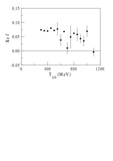
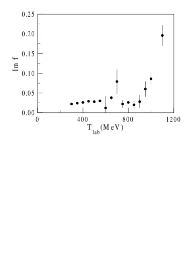
Figure 36: Real and imaginary parts of the the ${}^{3}D_{3}$ amplitude [236].

7.2.7 The NNN system

As a reliability test of the calculating scheme for the three-baryon system, the NNN bound-state problem has been studied. Of the three NNN states of table 13 only the channel $(S,I)=(1/2,1/2)$, that is the triton, has a bound state. By using the local potential a binding energy of 5.76 MeV is obtained, and 6.52 MeV with the non-local one. For comparison, we notice that the triton binding energy for the Reid-soft-core potential in the truncated T-matrix approximation is 6.58 MeV. Since the experimental value is $B_{\rm exp}=8.49$ MeV, the difference with the theoretical result, of about 3 MeV, is a measure of the uncertainty of the two-channel calculation in the case of the three-baryon system. A detailed study of the triton binding energy will be presented in the next section.

Table 17: Binding energies $B_{3}$ (in MeV) of the NNN, N$\Delta\Delta$, NN$\Delta$, and $\Delta\Delta\Delta$ states. ’ub’ denotes unbound channels. For the bound channels the separation energy is given below in parenthesis. $B_{3}^{L}$ ($B_{3}^{NL}$) refers to the local (nonlocal) potential.

		NNN		N$\Delta\Delta$		NN$\Delta$		$\Delta\Delta\Delta$
$S$	$I$	$B_{3}^{L}$	$B_{3}^{NL}$	$B_{3}^{L}$	$B_{3}^{NL}$	$B_{3}^{L}$	$B_{3}^{NL}$	$B_{3}^{L}$	$B_{3}^{NL}$
$1/2$	$1/2$	$\begin{array}[]{l}5.76\\ (2.63)\end{array}$	$\begin{array}[]{l}6.52\\ (4.38)\end{array}$	$-$	$-$	$-$	$-$	$\begin{array}[]{l}84.0\\ (53.5)\end{array}$	$\begin{array}[]{l}16.6\\ (9.2)\end{array}$
1/2	3/2	ub	ub	$-$	$-$	$-$	$-$	$\begin{array}[]{l}139.2\\ (0.7)\end{array}$	ub
3/2	1/2	ub	ub	$-$	$-$	ub	$\begin{array}[]{l}0.14\\ (0.002)\end{array}$	$\begin{array}[]{l}109.5\\ (1.1)\end{array}$	ub
3/2	3/2	$-$	$-$	$-$	$-$	ub	$\begin{array}[]{l}2.28\\ (0.14)\end{array}$	$-$	$-$
1/2	5/2	$-$	$-$	ub	$\begin{array}[]{l}0.63\\ (0.43)\end{array}$	$-$	$-$	$-$	$-$
5/2	1/2	$-$	$-$	ub	$\begin{array}[]{l}8.16\\ (0.36)\end{array}$	$-$	$-$	$\begin{array}[]{l}39.1\\ (8.6)\end{array}$	$\begin{array}[]{l}9.3\\ (1.9)\end{array}$
5/2	5/2	$-$	$-$	ub	$\begin{array}[]{l}0.18\\ (0.04)\end{array}$	$-$	$-$	$-$	$-$
1/2	7/2	$-$	$-$	$-$	$-$	$-$	$-$	$\begin{array}[]{l}6.3\\ (0.6)\end{array}$	ub
7/2	1/2	$-$	$-$	$-$	$-$	$-$	$-$	$\begin{array}[]{l}31.7\\ (1.2)\end{array}$	$\begin{array}[]{l}7.8\\ (0.4)\end{array}$
7/2	3/2	$-$	$-$	$-$	$-$	$-$	$-$	$\begin{array}[]{l}35.1\\ (4.6)\end{array}$	$\begin{array}[]{l}9.8\\ (2.0)\end{array}$

7.2.8 The NN$\Delta$ system

Though the presence of bound states in the N$\Delta$ $(j,i)=(2,1)$ and NN $(j,i)=(1,0)$ channels could induce to expect several bound states in the N$\Delta\Delta$ system, this is not the case indeed. As a matter of fact, with the non-local potential only two out of nine possible three-body states given in table 14 are bound. Because of the attractive contribution of the N$\Delta$ $(j,i)=(2,1)$ bound state with the non-local model, the three-body state $(3/2,1/2)$ turns out to be very weakly bound, with an energy of 0.14 MeV, and a separation energy different hardly from zero. This means that the $(S,I)=(3/2,1/2)$ state is very near the NN$\Delta$ threshold and therefore it represents the tribaryon resonance with the lowest possible mass since it can decay into three nucleons and one pion. Also, for this case the three-body state $(3/2,3/2)$ is bound. As it can be seen from table 14 this state has the contribution of all the two-body N$\Delta$ and NN channels. In spite of the fact that the N$\Delta$ two-body channels $(j,i)=(1,1)$ and $(2,2)$ present Pauli blocking, the attractive contribution of the N$\Delta$ $(j,i)=(2,1)$ and NN $(j,i)=(1,0)$ channels results to be enough to weakly bound this state. We note that neither one of the three-body states $(S,I)=(3/2,1/2)$ and $(3/2,3/2)$ is bound with the local interaction.

The predicted NN$\Delta$ states with $(S,I)=(3/2,1/2)$ and $(S,I)=(3/2,3/2)$ which correspond to $M\approx 3.4$ GeV are the tribaryon resonances with the lowest mass and therefore the ones that would be more easy to detect experimentally.

7.2.9 The N$\Delta\Delta$ system

In the non-local case one finds that three of the sixteen possible N$\Delta\Delta$ states given in table 15 are bound. They are the $(S,I)=(1/2,5/2)$, $(5/2,1/2)$, and $(5/2,5/2)$ states and their bound state energies are 0.63 MeV, 8.16 MeV, and 0.18 MeV, respectively. In the case of the states $(S,I)=(1/2,5/2)$ and $(S,I)=(5/2,1/2)$ the repulsive barrier due to the quark Pauli blocked N$\Delta$ states $(j,i)=(1,1)$ and $(2,2)$ is less strong than the attraction due to the state $(j,i)=(2,1)$, so that they result to be bound in the non-local model. The state $(S,I)=(5/2,5/2)$ is the weakest bound state of this system, since in addition to the contribution of the N$\Delta$ quark Pauli blocked channels, there exists that of the $\Delta\Delta$ quark Pauli blocked channels $(j,i)=(2,3)$ and $(3,2)$. This confirms what has been mentioned that it is the structure of the interaction of the two-body system the one which largely determines the three-body spectrum. Thus, the non-local interaction predicts the bound states $(S,I)=(1/2,5/2)$, $(5/2,1/2)$ and $(5/2,5/2)$, which in principle may be observed as tribaryon resonances which decay into three nucleons and two pions with masses close to the N$\Delta\Delta$ threshold.

7.2.10 The $\Delta\Delta\Delta$ system

While the non-local model presents four bound states the local interaction finds seven. From table 17 one observes that the three states which are missing in the non-local version are barely bound in the local version, i.e., they have very small separation energies. Since the non-local interaction tends to lower the attraction in all the $\Delta\Delta\Delta$ channels it is not surprising that those which were barely bound have disappeared. The more strongly bound three-body state (that is, the one with the largest separation energy) is the $(S,I)=(1/2,1/2)$ state which has precisely the triton quantum numbers. This shows again, like in the $\Delta\Delta$ and NN systems, the similarity between the $\Delta\Delta\Delta$ and NNN systems.

The reason why the $(S,I)=(1/2,1/2)$ state is the more strongly bound is very simple. As shown in table 13 this is the only state where none of the Pauli blocked two-body channels $(j,i)=(2,3)$ and $(3,2)$ contribute. In all the other three-body states the strong repulsion of these channels either completely destroys the bound state or allows just a barely bound one. The state $(S,I)=(7/2,3/2)$ comes next with respect to the separation energy. This state has a somewhat anomalous behaviour since it has a relatively large separation energy. This behaviour is sort of accidental and it can be understood as follows. As seen in table 13, there are four two-body channels contributing to the $(S,I)=(7/2,3/2)$ state, the two attractive ones $(j,i)=(2,1)$ and $(3,0)$ and the two repulsive ones $(j,i)=(2,3)$ and $(3,2)$. However, as seen in table 16 the attractive channels $(2,1)$ and $(3,0)$ have bound states at $E=-7.4$ MeV and $E=-7.8$ MeV, respectively, for the non-local model, and $E=-30.5$ MeV and $E=-29.9$ MeV, respectively, for the local one, so that the poles in the scattering amplitude of these two channels are very close together and therefore there is a reinforcement between them, giving rise to the anomalously large separation energy

7.3 The triton binding energy

The relevance and/or necessity of considering the non-local part of NN potentials in realistic interactions is still under debate. Over the past few years several studies have appeared in the literature which stress the potential importance of non-local effects for the quantitative understanding of few-body observables and, specifically, for the triton binding energy [245, 121, 242, 243, 244, 241, 240]. However, the majority of these investigations [242, 243, 244, 241, 240] explore only non-localities arising from the baryonic meson-exchange picture of the NN interaction.

The non-localities generated in a quark-model derivation of baryonic potentials may be relevant for the three-nucleon bound state. It has been argued that the assumptions associated with meson-exchange models sharply limit the nature of the off-shell properties of those potentials, once the on-shell matrix elements are constrained to fit the NN data [246]. Therefore, it is very interesting to investigate the off-shell features of potentials derived from a quark-model. Some studies in this direction were done in reference [245], but only the short-range part of the interaction was obtained by quark-model techniques, the intermediate and long-range parts being described by standard meson-exchanges between baryons. Accordingly, that work allowed only very limited conclusions with regard to effects of the quark substructure.

The triton binding energy has been studied in detail by means of the chiral constituent quark model [80]. The calculation has been done in a momentum-space Faddeev formalism restricted to the ${}^{1}S_{0}$ and ${}^{3}S_{1}-{}^{3}\!D_{1}$ NN partial waves, those which provide the bulk contribution to the three-nucleon binding energy. To solve the three-body Faddeev equations in momentum space a separable finite-rank expansion of the NN(coupled to N$\Delta)$ sector utilizing the EST method [247] is first performed. Such a technique has been extensively studied in other works for various realistic NN potentials [249] and specifically for a model including the coupling to the N$\Delta$ system [250]. In these works it was shown that, with a separable expansion of sufficiently high rank, reliable and accurate results on the three-body level can be achieved. In the present case it turns out that separable representations of rank 6 (for ${}^{1}S_{0}-(^{5}D_{0})$ and for ${}^{3}S_{1}-{}^{3}\!D_{1}$) are sufficient to get converged results. We refer the reader to references [249, 250, 251] for technical details on the expansion method. The quality of the separable expansion on the NN sector is very good. The phase shifts for the original non-local potential and for the corresponding separable expansion are almost indistinguishable [80].

Table 18: Triton binding energy, $E_{B}$ ($E_{\rm Exp}=-8.49$ MeV), and wave function components: $P_{S}$ is the $L=0$ symmetric spatial probability, $P_{S^{\prime}}$ the $L=0$ mixed symmetric spatial probability, $P_{P}$ the $L=1$ probability and $P_{D}$ the $L=2$ probability.

• 	CCQM [80]	Nijm II [248]	Bonn B [249]
  $E_{B}$ (MeV)	$-$7.72	$-$7.65	$-$8.17
  $P_{S}$ ($\%$)	91.49	90.33	91.35
  $P_{S^{\prime}}$ ($\%$)	1.430	1.339	1.368
  $P_{P}$ ($\%$)	0.044	0.064	0.049
  $P_{D}$ ($\%$)	7.033	8.267	7.235

Results for the triton are summarized in table 18. It is reassuring to see that the predicted value of the triton binding energy is comparable to the values obtained from conventional NN potentials, such as the Bonn or Nijmegen models. Thus, these calculations show that quark model based NN interactions are definitely able to provide a realistic description of the triton. The results also give support to the use of such interaction model for further few-body calculations. One should not forget at this point that the number of free parameters is greatly reduced as compared, for example, to effective theories, and, in addition, they are strongly correlated by the requirement of describing the baryon spectrum.

One can find in the literature other quark-inspired analysis of the triton binding energy. Some preliminary studies were done in Ref. [245] with a hybrid model as mentioned above. Recently the triton has been studied with the same quark model approach of Ref. [47], used for the study of the NN phase shifts (see section 5.3.5). A 34-channel calculation is done. The result obtained, $-$8.390 MeV [121], is pretty close to experiment. Although this model is only intended for the study of the baryon-baryon interaction, i.e., the connection with the one-body problem is lost, the quality of its predictions is remarkable.

8 Summary

We have reviewed recent calculations of few-body systems within a chiral constituent quark model framework. As for the moment an exact solution of QCD is not attainable, models incorporating its basic symmetries and some dynamics reveal as an important alternative to study low-energy hadron phenomenology. In this energy regime, confinement and chiral symmetry breaking appear as the most important properties of QCD. When properly implemented by means of chiral constituent quark models, the interplay between gluons, Goldstone bosons and constituent quarks is able to provide a consistent description of the baryon structure and properties and the baryon-baryon phenomenology. Several aspects of chiral constituent quark models in their application to study few-body systems deserve to be emphasized.

First, their universality in a double sense: on the one hand they allow to describe a great variety of phenomena (regarding N, NN and NNN systems) in terms of the same interacting potential, on the other hand once the very few parameters of the models are determined in the well-known NN system they allow to predict in a parameter-free way the spectrum and the interaction involving any other baryonic resonances.

Second, quark antisymmetry is properly implemented showing up as cluster antisymmetry and quark exchange between clusters. Its interplay with quark dynamics provides an elegant explanation of the observed hard core of the NN force. Similarly a precise description of the quark Pauli short-range repulsion appearing in other systems is obtained.

Third, these models at their current status have raised a degree of accuracy that allows to reproduce fine properties of two and three-baryon systems, like deuteron properties, the triton binding energy or charge symmetry breaking, with similar quality to baryonic meson-exchange models. Furthermore, the non-strange baryon spectrum is nicely reproduced once some relativistic effects are taken into account.

Despite this success a lot of work is still to be done. The confining interaction lacks a fundamental description and the phenomenological constraints are not enough to determine its properties. This has an important influence on the spin-orbit force which for the moment is not correctly described. Moreover, a complete relativistic treatment should be properly implemented and its consequences analyzed. Finally, other systems like mesons or multiquark systems should be studied within the same scheme. Meanwhile one can safely conclude that chiral constituent quark models have contributed in the last twenty years to a better understanding of the baryonic phenomenology.

References

References

- [1] Fritzsch H, Gell-Mann M and Leutwyler H 1973 Phys. Lett.B 47 365 Marciano W and Pagels H 1978 Phys. Rep. 36C 137
- [2] Montvay I and Munster G 1994 Quantum Fields on a Lattice (UK: Cambridge)
- [3] Weinberg S 1979 Physica A 96 327
- [4] Gasser J and Leutwyler H 1984 Ann. Phys., NY158 142
- [5] Isgur N and Wise M B 1989 Phys. Lett.B 232 113
- [6] Thacker B A and Lepage G P 1991 Phys. Rev.D 43 196
- [7] ’t Hooft G 1974 Nucl. Phys.B 72 461
- [8] Witten E 1979 Nucl. Phys.B 160 57
- [9] Zahed I and Brown G 1986 Phys. Rep. 142 2
- [10] Diakonov D, Petrov V and Polyakov M 1997 Z. Phys.A 359 305
- [11] Gell-Mann M 1964 Phys. Lett.8 214
- [12] Zweig G 1964 CERN Preprints 411 and 412 (unpublished)
- [13] Dalitz R H 1965 High Energy Physics (New York: Gordon and Breach) p 253
- [14] Greenberg O W 1964 Phys. Rev. Lett.13 598
- [15] Han M Y and Nambu Y 1965 Phys. Rev.139 1006
- [16] de Rújula A, Georgi H and Glashow S L 1975 Phys. Rev.D 12 147
- [17] Appelquist T, de Rújula A, Politzer H D and Glashow S L 1975 Phys. Rev. Lett.34 365
- [18] Eichten E, Gottfried K, Kinoshita T, Kogut J B, Lane K D and Yan T M 1975 Phys. Rev. Lett.34 369
- [19] Isgur N and Karl G 1978 Phys. Rev.D 18 4187 Isgur N and Karl G 1979 Phys. Rev.D 19 2653 Isgur N and Karl G 1979 Phys. Rev.D 20 1191
- [20] Bhaduri R K, Cohler L E and Nogami Y 1981 Nuovo CimentoA 65 376
- [21] Silvestre-Brac B and Gignoux C 1985 Phys. Rev.D 32 743
- [22] Chodos A, Jaffe R L, Johson K, Thorn C B and Weisskopf V F 1974 Phys. Rev.D 9 3471 DeGrand T, Jaffe R L, Johnson K and Kiskis J E 1975 Phys. Rev.D 12 2060
- [23] Chodos A and Thorn C B 1975 Phys. Rev.D 12 2733 Brown G E and Rho M 1979 Phys. Lett.B 82 177 Brown G E, Rho M and Vento V 1979 Phys. Lett.B 84 383 Théberge S, Thomas A W and Miller G A 1980 Phys. Rev.D 22 2838
- [24] Godfrey S and Isgur N 1985 Phys. Rev.D 32 189 Capstick S and Isgur N 1986 Phys. Rev.D 34 2809
- [25] Liberman D A 1977, Phys. Rev.D 16 1542
- [26] Neudatchin V G, Smirnov Yu F and Tamagaki R 1977 Prog. Theor. Phys. 58 1072
- [27] Toki H 1980 Z. Phys.A 294 173
- [28] Ribeiro J E T 1980 Z. Phys.C 5 27
- [29] Oka M and Yazaki K 1980 Prog. Theor. Phys. 66 556
- [30] Oka M and Yazaki K 1980 Phys. Lett.B 90 41
- [31] Harvey M 1981 Nucl. Phys.A 352 326
- [32] Faessler A, Fernández F, Lübeck G and Shimizu K 1982 Phys. Lett.B 112 201 Faessler A, Fernández F, Lübeck G and Shimizu K 1983 Nucl. Phys.A 402 555
- [33] Cvetic M, Golli B, Mankoc-Borstnik N and Rosina M 1983 Nucl. Phys.A 395 349
- [34] Fujiwara Y and Hecht K T 1986 Phys. Lett.B 171 17
- [35] Oka M and Yazaki K 1983 Nucl. Phys.A 402 477
- [36] Fujiwara Y and Hecht K T 1986 Nucl. Phys.A 462 621
- [37] Manohar A and Georgi H 1984 Nucl. Phys.B 234 189
- [38] Diakonov D and Petrov V Yu 1984 Nucl. Phys.B 245 259
- [39] Diakonov D 1996 Preprint hep-ph/9602375
- [40] Shimizu K 1984 Phys. Lett.B 148 418
- [41] Bräuer K, Faessler A, Fernández F and Shimizu K 1985 Z. Phys.A 320 609 Bräuer K, Faessler A, Fernández F and Shimizu K 1990 Nucl. Phys.A 507 599
- [42] Obukhovsky I T and Kusainov A M 1990 Phys. Lett.B 238 142
- [43] Fernández F, Valcarce A, Straub U and Faessler A 1993 J. Phys. G: Nucl. Part. Phys.19 2013
- [44] Valcarce A, González P, Fernández F and Vento V 1996 Phys. Lett.B 367 35
- [45] Glozman L Ya and Riska D O 1996 Phys. Rep. 268 263
- [46] Nakamoto C and Toki H 1998 Prog. Theor. Phys. 99 1001
- [47] Fujiwara Y, Nakamoto C and Suzuki Y 1996 Phys. Rev.C 54, 2180 Fujiwara Y, Fujita T, Kohno M, Nakamoto C and Suzuki Y 2002 Phys. Rev.C 65, 014002
- [48] Fujiwara Y, Miyagawa K, Khono M, Suzuki Y and Nakamoto C 2004 Nucl. Phys.A 737 243 Fujiwara Y, Fujita T, Nakamoto C, Suzuki Y and Khono M 1998 Nucl. Phys.A 639 41c Fujiwara Y, Khono M, Nakamoto C and Suzuki Y 2001 Phys. Rev.C 64 054001
- [49] Garcilazo H and Valcarce A 2003 Phys. Rev.C 68 035207
- [50] Theussl L, Amghar A, Desplanques B and Noguera S 2003 Few-Body Syst. Supp. 14 393 Amghar A, Desplanques B and Theussl L 2003 Phys. Lett.B 574 201 Glozman L Ya, Radici M, Wagenbrunn R F, Boffi S, Klink W and Plessas W 2001 Phys. Lett.B 516 183 Desplanques B 2004 Preprint nucl-th/0405059 Desplanques B 2004 Preprint nucl-th/0405060 Desplanques B 2004 Preprint nucl-th/0407074 Melde T, Canton L, Plessas W and Wagenbrunn R F 2004 Preprint hep-ph/0411322
- [51] Bali G S 2001 Phys. Rep. 343 1
- [52] Shimizu K 1989 Rep. Prog. Phys.52 1
- [53] Yndurain F J 1999 The Theory of Quark and Gluon Interactions (Berlin: Springer)
- [54] Pich A 1995 Preprint hep-ph/9505231
- [55] Goldstone J 1961 Nuovo Cimento19 154
- [56] Bhaduri R K, Cohler L E and Nogami Y 1980 Phys. Rev. Lett.44 1369
- [57] Yazaki K 1990 Prog. Part. Nucl. Phys. 24 353
- [58] Fernández F, Valcarce A, González P and Vento V 1992 Phys. Lett.B 287 35 Fernández F, Valcarce A, González P and Vento V 1994 Nucl. Phys.A 567 741
- [59] Scadron M D 1993 Phys. At. Nucl. 56 1595
- [60] Liu G Q, Swift M, Thomas A W and Holinde K 1993 Nucl. Phys.A 556 331
- [61] Ericson T E O 1992 Nucl. Phys.A 543 409c
- [62] Valcarce A, Buchmann A, Fernández F and Faessler A 1994 Phys. Rev.C 50 2246
- [63] Stancu F 1996 Group Theory in Subnuclear Physics (Oxford: Clarendon Press)
- [64] Holinde K 1984 Nucl. Phys.A 415 477
- [65] Suzuki Y and Hecht K T 1984 Nucl. Phys.A 420 525
- [66] Valcarce A, Fernández F, González P and Vento V 1995 Phys. Rev.C 52 38
- [67] Juliá-Díaz B, Fernández F, González P and Valcarce A 2001 Phys. Rev.C 63 024006
- [68] Ferreira E and Dosch H G 1989 Phys. Rev.C 40 1750
- [69] Myhrer F and Wroldsen J 1986 Phys. Lett.B 174 366 Myhrer F and Wroldsen J 1988 Rev. Mod. Phys.60 629
- [70] Saito S 1969 Prog. Theor. Phys. 41 705
- [71] Valcarce A, Fernández F and González P 1997 Phys. Rev.C 56 3026
- [72] Hecht K T and Pang S C 1969 J. Math. Phys. 10 1571
- [73] Valcarce A, Buchmann A, Fernández F and Faessler A 1995 Phys. Rev.C 51 1480
- [74] Yu Y W, Zhang Z Y, Shen P N and Dai L R 1995 Phys. Rev.C 52 3393
- [75] Wheeler J A 1937 Phys. Rev.52 1107
- [76] Tang Y C, LeMere M and Thompsom D R 1978 Phys. Rep. 47 167
- [77] Kamimura M 1977 Prog. Theor. Phys. Supp. 62 236
- [78] DeTar C 1978 Phys. Rev.D 17 323
- [79] Oka M and Yazaki K 1984 Int. Rev. Nucl. Phys. 1 489
- [80] Juliá-Díaz B, Haidenbauer J, Valcarce A and Fernández F 2002 Phys. Rev.C 65 034001
- [81] Buchmann A, Yamauchi Y and Faessler A 1989 Nucl. Phys.A 496 621
- [82] Juliá-Díaz B, Valcarce A, González P and Fernández F 2003 Eur. Phys. J. A 19 s01,99
- [83] Jain B K and Santra A B 1993 Phys. Rep. 230 1
- [84] Sauer P U 1986 Prog. Part. Nucl. Phys. 16 35
- [85] Lomon E L 1982 Phys. Rev.D 26 576
- [86] Peña M T, Garcilazo H, Oelfke U and Sauer P U 1992 Phys. Rev.C 45 1487
- [87] Peña M T, Henning H and Sauer P U 1990 Phys. Rev.C 42 855
- [88] Alexandrou C and Blankleider B 1990 Phys. Rev.C 42 517
- [89] Takaki T and Thies M 1988 Phys. Rev.C 38 2230
- [90] Garcilazo H, Mizutani T, Peña M T and Sauer P U 1990 Phys. Rev.C 42 2315
- [91] Valcarce A, Fernández F, Garcilazo H, Peña M T and Sauer P U 1994 Phys. Rev.C 49 1799
- [92] Shypit R L, Bugg D V, Sanjari A H, Lee D M, McNaughton M W, Silbar R R, Hollas C L, McNaughton K H, Riley P and Davis C A 1989 Phys. Rev.C 40 2203 Shypit R L, Bugg D V, Lee D M, McNaughton M W, Silbar R R, Stewart N M, Clough A S, Hollas C L, McNaughton K H, Riley P and Davis C A 1988 Phys. Rev. Lett.60 901
- [93] Allasia D et al1986 Phys. Lett.B 174 450
- [94] Haidenbauer J, Holinde K and Johnson M B 1993 Phys. Rev.C 48 2190
- [95] Oka M 1993 Frontiers Science Series No. 6, p 950
- [96] Wang F, Wu G, Teng L and Goldman T 1992 Phys. Rev. Lett.69 2901
- [97] Goldman T, Maltman K, Stephenson Jr. G J, Schmidt K E and Wang F 1989 Phys. Rev.C 39 1889
- [98] Cvetič M, Golli B, Mankoč-Borštnik N and Rosina M 1980 Phys. Lett.B 93 489
- [99] Garcilazo H, Fernández F, Valcarce A and Mota R D 1997 Phys. Rev.C 56 84
- [100] Hagiwara K et al2002 Phys. Rev.D 66 010001
- [101] Arenhövel H, Danos M and Williams H T 1971 Nucl. Phys.A 162 12
- [102] Hamada T and Johnston I D 1962 Nucl. Phys.34 382
- [103] Reid R V 1968 Ann. Phys., NY50 411
- [104] Rost E 1975 Nucl. Phys.A 249 510
- [105] Peña M T, Riska D O and Stadler A 1999 Phys. Rev.C 60 045201
- [106] Coon S A, Peña M T and Riska D O 1995 Phys. Rev.C 52 2925
- [107] Hirenzaki S, Oset E and Fernández de Cordoba P 1996 Phys. Lett.B 378 29 Hirenzaki S, Fernández de Cordoba P and Oset E 1996 Phys. Rev.C 53 277
- [108] Álvarez-Ruso L 1999 Phys. Lett.B 452 207
- [109] Garcilazo H and Moya de Guerra E 1993 Nucl. Phys.A 562 521
- [110] Juliá-Díaz B, Valcarce A, González P and Fernández F 2002 Phys. Rev.C 66 024005
- [111] Riska D O and Brown G E 2001 Nucl. Phys.A 679 577
- [112] Huber S and Aichelin J 1994 Nucl. Phys.A 573 587
- [113] Soyeur M 2000 Nucl. Phys.A 671 532
- [114] Machleidt R 1989 Adv. Nucl. Phys. 19 189
- [115] Ordóñez C, Ray L and van Kolck U 1996 Phys. Rev.C 53 2086
- [116] Wakamatsu M, Yamamoto R and Yamauchi Y 1984 Phys. Lett.B 146 148
- [117] Vinh Mau R, Semay C, Loiseau B and Lacombe M 1991 Phys. Rev. Lett.67 1392
- [118] Lacombe M, Loiseau B, Richard J M, Vinh Mau R, Côté J. Pirès P and de Tourreil R 1980 Phys. Rev.C 21 861
- [119] Takeuchi S, Shimizu K and Yazaki K 1989 Nucl. Phys.A 504 777
- [120] Valcarce A, Faessler A and Fernández F 1995 Phys. Lett.B 345 367
- [121] Fujiwara Y, Miyagawa K, Kohno M, Suzuki Y and Nemura H 2002 Phys. Rev.C 66 021001
- [122] Stoks V G J, Klomp R A M, Terheggen C P F and de Swart J J 1994 Phys. Rev.C 49 2950
- [123] Entem D R, Fernández F and Valcarce A 1999 Phys. Lett.B 463 153
- [124] Matveev V A and Sorba P 1977 Lett. Nuov. Cim. 20 435
- [125] González P and Vento V 1987 Few-Body Syst. 2 145
- [126] Kerman A K and Kisslinger L S 1969 Phys. Rev.180 1483
- [127] Hadjimichael E 1973 Phys. Lett.B 46 147
- [128] Denisov O Yu, Kuksa S D and Lykasov G I 1999 Phys. Lett.B 458 415
- [129] Dorodnykh Yu L, Lykasov G I, Rzyanin M V and Cassing W 1995 Phys. Lett.B 346 227
- [130] Uzikov Yu N 1997 Phys. At. Nucl. 60 1458 Uzikov Yu N 1997 Phys. At. Nucl. 60 1616
- [131] Kusainov A M, Neudatchin V G and Obukhovsky I T 1991 Phys. Rev.C 44 2343
- [132] Glozman L Ya and Kuchina E I 1994 Phys. Rev.C 49 1149
- [133] Zhang Z Y, Bräuer K, Faessler A and Shimizu K 1985 Nucl. Phys.A 443 557
- [134] Maeda I, Arima M and Masutani K 2000 Phys. Lett.B 474 255
- [135] Entem D R, Fernández F and Valcarce A 2000 Phys. Rev.C 62 034002
- [136] Juliá-Díaz B, Entem D R, Valcarce A and Fernández F 2002 Phys. Rev.C 66 047002
- [137] Arenhövel H 1975 Z. Phys.A 275 189
- [138] Dymarz R and Khanna F C 1990 Nucl. Phys.A 516 549
- [139] Haapakoski P and Saarela M 1974 Phys. Lett.B 53 333
- [140] Green A M and Haapakoski P 1974 Nucl. Phys.A 221 429
- [141] Sitarski W P, Blunden P G and Lomon E L 1987 Phys. Rev.C 36 2479
- [142] SAID program. Available on the web site http://gwdac.phys.gwu.edu
- [143] Kaiser N, Gerstendörfer S and Weise W 1998 Nucl. Phys.A 637 395
- [144] Kaiser N, Brockmann R and Weise W 1997 Nucl. Phys.A 625 758
- [145] Helminen C and Riska D O 1998 Phys. Rev.C 58 2928
- [146] Suzuki Y and Hecht K T 1984 Phys. Rev.C 29 1586
- [147] Faessler A, Buchmann A and Yamauchi Y 1993 Int. J. Mod. Phys. E 2 39
- [148] Morimatsu O, Yazaki K and Oka M 1984 Nucl. Phys.A 424 412
- [149] Koike Y 1986 Nucl. Phys.A 454 509 Koike Y, Morimatsu O and Yazaki K 1986 Nucl. Phys.A 449 635
- [150] Machleidt R, Holinde K and Elster C 1987 Phys. Rep. 149 1
- [151] Morimatsu O, Ohta S, Shimizu K and Yazaki K 1984 Nucl. Phys.A 420 573
- [152] Zhang Z Y, Faessler A, Straub U and Glozman L Ya 1994 Nucl. Phys.A 578 573
- [153] Miller G A, Nefkens B M K and Slaus I 1990 Phys. Rep. 194 1
- [154] Stephenson Jr. G J, Maltman K and Goldman T 1991 Phys. Rev.D 43 860
- [155] Pöpping H, Sauer P U and Xi-Zhen Z 1987 Nucl. Phys.A 474 557
- [156] Garcilazo H and Mizutani T 1990 Systems (Singapore: World Scientific)
- [157] Le Yaouanc A, Oliver L, Pène O and Raynal J C 1988 Hadron Transitions in the Quark Model (New York: Gordon and Breach)
- [158] Entem D R, Fernández F and Valcarce A 2003 Phys. Rev.C 67 014001
- [159] Arndt R A, Oh C H, Strakovsky I I and Workman R L 1997 Phys. Rev.C 56 3005
- [160] Gutbrod F and Montvay I 1984 Phys. Lett.B 136 411
- [161] Isgur N 2000 Phys. Rev.D 62 054026 Isgur N 2000 Preprint nucl-th/0007008
- [162] Desplanques B, Gignoux C, Silvestre-Brac B, González P, Navarro J and Noguera S 1992 Z. Phys.A 343 331
- [163] Garcilazo H, Valcarce A and Fernández F 2001 Phys. Rev.C 64 058201
- [164] Feshbach H and Rubinow S I 1955 Phys. Rev.98 188
- [165] Suzuki Y and Varga K 1998 Stochastic Variational Approach to Quantum-Mechanical Few-Body Problems (Berlin: Springer)
- [166] Faddeev L D 1961 Sov. Phys.-JETP 12 1014
- [167] Papp Z 1999 Few-Body Syst. 26 99
- [168] Papp Z, Krassnigg A and Plessas W 2000 Phys. Rev.C 62 044004
- [169] Garcilazo H 2003 Phys. Rev.C 67 055203
- [170] Glozman L Ya, Plessas W, Varga K and Wagenbrunn R F 1998 Phys. Rev.D 58 094030
- [171] Dziembowski Z, Fabre de la Ripelle M and Miller G A 1996 Phys. Rev.C 53 2038
- [172] Glozman L Ya, Papp Z, Plessas W, Varga K and Wagenbrunn R F 1998 Phys. Rev.C 57 3406
- [173] Garcilazo H, Valcarce A and Fernández F 2001 Phys. Rev.C 63 035207
- [174] Basdevant J L and Boukraa S 1986 Z. Phys.C 30 103
- [175] Carlson J, Kogut J and Pandharipande V R 1983 Phys. Rev.D 27 233
- [176] Furuichi M and Shimizu K 2002 Phys. Rev.C 65 025201
- [177] Dong Y, Su J and Wu S 1994 J. Phys. G: Nucl. Part. Phys.20 73
- [178] Löring U, Kretzschmar K, Metsch B Ch and Petry H R 2001 Eur. Phys. J. A 10 309
- [179] Löring U, Metsch B Ch and Petry H R 2001 Eur. Phys. J. A 10 395
- [180] Löring K, Metsch B Ch and Petry H R 2001 Eur. Phys. J. A 10 447
- [181] Jena S N, Behera M R and Panda S 1998 J. Phys. G: Nucl. Part. Phys.24 1089
- [182] Nakano T et al2003 Phys. Rev. Lett.91 012002
- [183] Nakano T 2004 Presented at QNP2004
- [184] Barmin V V et al2003 Phys. At. Nucl. 66 1715
- [185] Stepanyan S et al2003 Phys. Rev. Lett.91 252001
- [186] Barth J et al2003 Phys. Lett.B 572 127
- [187] Kubarovsky V 2003 Phys. Rev. Lett.92 032001
- [188] Asratyan A E 2004 Phys. At. Nucl. 67 682
- [189] Aleev A 2004 Preprint hep-ex/0401024
- [190] Airapetian A 2004 Phys. Lett.B 585 213
- [191] ZEUS Collaboration 2004 Phys. Lett.B 591 7
- [192] Abdel-Bary M 2004 Phys. Lett.B 595 127
- [193] Knöpfle K T et al2004 J. Phys. G: Nucl. Part. Phys.30 S1363
- [194] Bai J Z et al2004 Phys. Rev.D 70 012004
- [195] Litvintsev D 2004 Preprint hep-ex/0410024
- [196] Aubert B et al2004 Preprint hep-ex/0408064
- [197] Schael S et al2004 Phys. Lett.B 599 1
- [198] Lin C 2004 Presented at ICHEP2004
- [199] Christian D et al2004 Presented at QNP2004
- [200] Longo M et al2004 Phys. Rev.D 70 111101
- [201] Pinkenburg C et al2004 J. Phys. G: Nucl. Part. Phys.30 S1201
- [202] Mizuk R et al2004 Preprint hep-ex/0411005
- [203] Stenson K 2004 Preprint hep-ex/0412021
- [204] Napolitano J, Cummings J and Witkowski M 2004 Preprint hep-ex/0412031
- [205] Armstrong S R 2004 Preprint hep-ex/0410080
- [206] Engelfried J 2004 Presented at Quark Confinement 2004
- [207] Antipov Yu M et al2004 Eur. Phys. J. A 21 455
- [208] Nussinov S 2004 Preprint hep-ph/0403028
- [209] Dzierba A R, Meyer C A and Szczepaniak A P 2004 Preprint hep-ex/0412077
- [210] Dzierba A R, Krop D, Swat M, Szczepaniak A P and Teige S 2004 Phys. Rev.D 69 051901
- [211] Jaffe R L 2004 Eur. Phys. J. C 35 221
- [212] Praszalowicz M 1987 Skyrmions and Anomalies (Singapore: World Scientific) p 112
- [213] Jaffe R L and Wilczek F 2003 Phys. Rev.L 91 232003
- [214] Karliner M and Lipkin H J 2003 Preprint hep-ph/0307243
- [215] Glozman L Ya 2003 Phys. Lett.B 575 18
- [216] Stancu Fl and Riska D O 2003 Phys. Lett.B 575 242
- [217] Mulders P J, Aerts A T and de Swart J J 1980 Phys. Rev.D 21 2653
- [218] Maltman K 1985 Nucl. Phys.A 438 669
- [219] Wang F, Ping J and Goldman T 1995 Phys. Rev.C 51 1648
- [220] Wong C W 1998 Phys. Rev.C 57 1962
- [221] Buchmann A J, Wagner G and Faessler A 1998 Phys. Rev.C 57 3340
- [222] Yuan X Q, Zhang Z Y, Yu Y W and Shen P N 1999 Phys. Rev.C 60 045203
- [223] Mota R D, Valcarce A, Fernández F and Garcilazo H 1999 Phys. Rev.C 59 46
- [224] Garcilazo H, Valcarce A and Fernández F 1999 Phys. Rev.C 60 044002
- [225] Mota R D, Valcarce A, Fernández F, Entem D R and Garcilazo H 2002 Phys. Rev.C 65 034006
- [226] Cvetič-Krivec M, Golli B, Mankoč-Borštnik N and Rosina M 1981 Phys. Lett.B 99 486
- [227] Huber G M et al2000 Phys. Rev.C 62 044001
- [228] Maltman K and Isgur N 1984 Phys. Rev.D 29 952
- [229] Garcilazo H 1997 J. Phys. G: Nucl. Part. Phys.23 1101
- [230] Harper E P, Kim Y E and Tubis A 1972 Phys. Rev. Lett.28 1533
- [231] Berthold G H, Zankel H, Mathelitsch L and Garcilazo H 1986 Nuovo CimentoA 93 89
- [232] Chen C R, Payne G L, Friar J L and Gibson B F 1985 Phys. Rev. Lett.55 374
- [233] Afnan I R and Thomas A W 1974 Phys. Rev.C 10 109
- [234] Otsuki S, Tamagaki R and Yasuno M 1965 Prog. Theor. Phys. Supp. Number Extra 578
- [235] Hoshizaki N 1978 Prog. Theor. Phys. 60 1796 Hoshizaki N 1979 Prog. Theor. Phys. 61 129
- [236] Arndt R A, Strakovsky I I and Workman R L 2000 Phys. Rev.C 62 034005
- [237] Yokosawa A 1980 Phys. Rep. 64 47
- [238] Valcarce A, Garcilazo H, Mota R D and Fernández F 2001 J. Phys. G: Nucl. Part. Phys.27 L1
- [239] Kamae T and Fujita T 1977 Phys. Rev. Lett.38 471
- [240] Doleschall P and Borbély I 2000 Phys. Rev.C 62 054004
- [241] Elster Ch, Evans E E, Kamada H and Glöckle W 1996 Few-Body Syst. 21 25
- [242] Gibson B F, Kohlhoff H and von Geramb H V 1995 Phys. Rev.C 51 R465
- [243] Haidenbauer J and Holinde K 1996 Phys. Rev.C 53 R25
- [244] Machleidt R, Sammarruca F and Song Y 1996 Phys. Rev.C 53 R1483
- [245] Takeuchi S, Cheon T and Redish E F 1992 Phys. Lett.B 280 175
- [246] Redish E F and Stricker-Bauer K 1983 Phys. Lett.B 133 1
- [247] Ernst D J, Shakin C M, Thaler R M and Weiss D L 1973 Phys. Rev.C 8 2056
- [248] Friar J L, Payne G L, Stoks V G J and de Swart J J 1993 Phys. Lett.B 311 4
- [249] Schadow W, Sandhas W, Haidenbauer J and Nogga A 2000 Few-Body Syst. 28 241
- [250] Nemoto S, Chmielewski K, Schellingerhout N W, Sauer P U, Haidenbauer J and Oryu S 1998 Few-Body Syst. 24 213
- [251] Haidenbauer J and Plessas W 1983 Phys. Rev.C 27 63 Haidenbauer J and Plessas W 1984 Phys. Rev.C 30 1822