Non local lagrangians: the pion.

Abstract

We define a family of non local and chirally symmetric low energy lagrangians motivated by theoretical studies on Quantum Chromodynamics. These models lead to quark propagators with non trivial momentum dependencies. We define the formalism for two body bound states and apply it to the pion. We study the coupling of the photon and W bosons with special attention to the implementation of local gauge invariance. We calculate the pion decay constant recovering the Goldberger-Treiman and the Gell-Mann-Oakes-Renner relations. We recover a form of the axial current consistent with PCAC. Finally we study the pion form factor and we construct the operators involved in its parton distribution.

I Introduction.

The strong interaction among hadrons is supposed to be described by Quantum Chromodynamics (QCD) fgl which is a field theory defined in terms of quark and gluon fields. While the asymptotic behavior of QCD is well understood and its proponents worthy of the highest recognition nobel , the low energy behavior is still a subject of much scientific endeavor. Low energy physics seems to be ultimately governed by flavor dynamics. Confinement wilson , the property of QCD which describes how the dynamics based on color in the lagrangian transforms into a dynamics based on flavor for the physical states, and why these cannot exist with color charge, is still a subject of research and debate. This complex low energy behavior is described conventionally in terms of approximations to the theory, i.e., lattice QCD lattice , non relativistic QCD nrqcd , $1/N_{c}$ -expansion hooft or effective theories, i.e. Chiral Perturbation Theory gl , Heavy Quark Effective Theory hqet , etc. Models turn out to be extremely useful in some instances when the other approaches are too complex, i.e, non-relativistic quark models ik ; mg , bag models mit ; vento , Nambu-Jona Lasinio (NJL) model njl , chiral-soliton models skyrme ; vento1 ; diakonov , etc. Another method to study non perturbative physics in a lagrangian theory like QCD is to solve the Dyson-Schwinger equations. The application of this formalism to QCD becomes an enormously difficult task but progress, in understanding the theory from this approach, has been achieved RobertsWilliams94-97 ; AlkoferSmekal01 ; MarisRoberts03 . The global color model Tandy97 , the extended non-local NJL model Birse95 ; Birse98 ; Birse04 ; Osipov95 ; Osipov06 , and models using separable interactions GrossBuckIto91 has been introduced as model realizations of QCD in a field theory formalism.

One major problem is to understand the pion, because it is the system which contains all the ingredient of QCD: asymptotic freedom, confinement and spontaneously broken chiral symmetry. Chiral symmetry governs the static properties of the theory, like the quark condensate, the mass and decay constant of the pion. The dynamics fixes the internal structure of the pion, which is accessible through the pion electromagnetic form factor.

The pion form factor has been a subject of many studies. In relativistic quantum mechanics the pion form factor has a long history of debate IsgurLlewellyn ; ChungKoesterPolitzou ; CardarelliPaceSalmeSimula ; ChoiJi ; MeloNausFrederico . One of the main problems is the choice of one of the various Dirac forms DesplanquesNogueraTheussl ; AmgharDesplanquesTheussl . One of the most interesting conclusions is that results of a calculation depend not only on the Dirac form chosen but also on the frame chosen TheusslAmgharDesplanquesNog03 ; Desplanques . The reason for this is that the truncation needed in relativistic quantum mechanics to calculate form factors breaks Poincaré invariance.

A way to avoid this problem is to work in a field theory formalism. The pion form factor has also been studied within Dyson-Schwinger Equations schemes by several authors Roberts96 ; BurdenRobertsThomson96 ; MarisTandi00 . The starting point is in most treatments the pion Bether-Salpeter amplitude calculated in the rainbow approximation. The pion form factor is calculated using the so called impulse approximation which considers only the triangle diagram, and the use of a dressed vertex for the photon. For the latter the Ball-Chiu BallChiu80 expression for the vertex , or modified versions of it, have been used.

The pion form factor has been studied also for the non-local NJL model Birse98 . In this case the coupling of the photon is obtained by restoration of the gauge symmetry Birse95 ; Bos91 ; Osipov06 .

Our aim is to construct a model for hadron structure and hadronic interactions developing a formalism which preserves the fundamental symmetries of the theory (chiral, Poincaré and local electromagnetic gauge invariances) and which incorporates information coming from fundamental studies of Quantum Chromodynamics. For this purpose we want to define a formalism which contains the physical intuition of model calculations and the lagrangian formalism of the effective theories. To achieve this we have found that the best suited scheme is to describe the physics by mean of a phenomenological chirally invariant non local lagrangian.

Working in a lagrangian theory, the two main ingredients in a non perturbative analysis involving the pion are: i) the quark propagator, obeying the Dyson equation; ii) the description of the pion as a bound state of a Bethe-Salpeter equation (BSE). Due to chiral symmetry the kernels of these two equations are not independent DelbourgoScadron79 . Solving the Dyson equation for our lagrangian leads to momentum dependencies in the quark propagators through its mass and its wave function renormalization. In our scheme the gluons have been integrated out and we have only flavor interaction between quarks. Confinement is imposed by the structure of the quark propagator and by limiting the Fock space to color singlet states. The pion is obtained in a consistent way solving the BSE, and the Goldstone character of the pion is recovered.

Our model can be seen as an extension of the non-local NJL model Birse95 ; Birse98 ; Osipov95 ; Osipov06 , but with a particular philosophy. We consider the description of the quark propagator as the main ingredient. This is because the quark propagator is the first information that can be obtained from fundamental studies, as lattice QCD. Our lagrangian is the minimal extension which allows to incorporate the full momentum dependence of the quark propagator, through its mass and wave function renormalization. From this lagrangian we can explore what are the implications for other observables originated by changes in the quark propagator.

Our formalism implements the coupling of the photon in a gauge invariant manner Birse95 ; Bos91 ; Osipov06 . This allows to study the electromagnetic properties of the pion, which depend strongly on the quark-photon vertex. Usually this vertex is calculated by using the Ward-Takahashi identity BallChiu80 . This method fixes the longitudinal part of the vertex leaving the transverse part unconstrained. We show that this procedure does not guarantee local gauge invariance, while ours does. As an application we study the pion form factor, showing that the conventional impulse approximation, in which the form factor is calculated using the triangle diagram, is not consistent with local gauge symmetry.

In models based on field theory formalism, the construction of the axial current and the definition of the pion decay constant need particular attention. In ref MarisRobertsTandy98 a first expression for the axial current is given. In ref Birse95 ; Osipov06 additional contributions to the pion decay constant are included. In this paper we implement the coupling of quarks to the $W^{\mu}$ bosons in a gauge invariant manner following a procedure similar to the one used for photons. Then, we analyze the axial current and the pion decay constant.

Our formalism is very effective for building operators describing observables in a consistent way. As an application we have studied the operators involved in the parton distribution of the pion.

This paper is organized as follows. In section II we define our lagrangian, we discuss the quark propagator, and we fix the parameters in order to describe the adequate quark propagator obtained by more fundamental studies based on QCD. In section III we describe the pion state. In section IV we study the quark-photon vertex and recover the Ball-Chiu ansatz but with additional contributions. In section V we study the axial current and the pion decay constant. In section VI we apply the model to the study of the pion form factor. We show that a four quark-one photon vertex appears in a natural way. In section VII we obtain the contribution of this new term to the parton distribution operator. The last section contains the conclusions of our investigation.

II A phenomenological non local Lagrangian for hadron structure.

Let us build a model which produces a non trivial momentum dependence in the quark propagator and preserves all the required symmetries: Poincaré and chiral symmetry. This momentum dependence will arise from a lagrangian description and manifests itself as a quark momentum dependent mass and a quark momentum dependent wave function renormalization. Let us define the non local currents as

$$J_{\mathcal{O}}\left(x\right)=\int d^{4}y\,G\left(y\right)\bar{\psi}\left(x+\frac{1}{2}y\right)\mathcal{O}\psi\left(x-\frac{1}{2}y\right)\ ,$$ (II.1)

where the operator $\mathcal{O}$ is such that

$$\gamma^{0}\mathcal{O}^{\dagger}\gamma^{0}=\mathcal{O\ }.$$ (II.2)

With these definitions the hermiticity of the currents $\left(J_{\mathcal{O}}^{\dagger}\left(x\right)=J_{\mathcal{O}}\left(x\right)\right)$ implies that $G^{\dagger}\left(-y\right)=G\left(y\right).$ A local current corresponds to $G\left(y\right)=\delta^{4}\left(y\right)$ and thus the natural normalization for the functions $G\left(y\right)$ is

$$\int d^{4}y\,G\left(y\right)=1.$$ (II.3)

We build a lagrangian in terms of non local currents, preserving $U_{L}\left(2\right)\otimes U_{R}\left(2\right)$ chiral symmetry, and producing the desired momentum dependences as

$$\mathcal{L}\left(x\right)=\bar{\psi}\left(x\right)\left(i\ \hbox to0.0pt{$/$\hss}\partial-m_{0}\right)\psi\left(x\right)+g_{0}\left[J_{S}^{\dagger}\left(x\right)J_{S}\left(x\right)+\vec{J}_{5}^{\;\dagger}\left(x\right)\vec{J}_{5}\left(x\right)\right]+g_{p}J_{p}^{\dagger}\left(x\right)J_{p}\left(x\right)\ ,$$ (II.4)

where the currents are defined by

$$J_{S}\left(x\right) =\int d^{4}y\,G_{0}\left(y\right)\bar{\psi}\left(x+\frac{1}{2}y\right)\psi\left(x-\frac{1}{2}y\right)\ ,$$ (II.5)

$$\vec{J}_{5}\left(x\right) =\int d^{4}y\,G_{0}\left(y\right)\bar{\psi}\left(x+\frac{1}{2}y\right)i\vec{\tau}\gamma_{5}\psi\left(x-\frac{1}{2}y\right)\ ,$$ (II.6)

$$J_{p}\left(x\right) =\int d^{4}y\,G_{p}\left(y\right)\bar{\psi}\left(x+\frac{1}{2}y\right)\frac{1}{2}i\overleftrightarrow{\hbox to0.0pt{$/$\hss}\partial}\psi\left(x-\frac{1}{2}y\right)\ ,$$ (II.7)

where $u\overleftrightarrow{\partial}v=u\left(\partial v\right)-\left(\partial u\right)v.$ The transformation properties of the non local currents are the same as those of the local ones. The first and second currents require the same $G_{0}\left(y\right)$ to guarantee chiral invariance. The third current is self-invariant under chiral transformations. The scalar current, $J_{S},$ generates a momentum dependent mass, and the last current, the ”momentum” current, $J_{p},$ is responsible for the momentum dependence of the wave function renormalization. The pseudo-scalar current, $\vec{J}_{5},$ generates the pion pole. From now on, just for simplicity, we assume that all the $G\left(y\right)$ functions are real.

The interaction vertex obtained from the Lagrangian (II.4) automatically includes vertex form factors. Let us define

$$G\left(p\right)=\int d^{4}y\,e^{iyp}G\left(y\right)\ \ ,$$ (II.8)

with the normalization condition

$$G\left(p=0\right)=1.$$ (II.9)

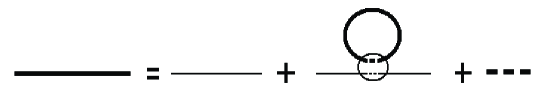
Figure 1: Diagrammatic representation of the quark propagator. The non local four quark vertex is represented by a circle with structure.

The full quark propagator is obtained from de Dyson equation, represented in Fig. 1,

$$S\left(p\right)=\frac{1}{\hbox to0.0pt{$/$\hss}p-m_{0}+\Sigma\left(p\right)+i\epsilon}\ \ ,$$ (II.10)

with

$$\Sigma\left(p\right)=-\alpha_{0}\ G_{0}\left(p\right)-\hbox to0.0pt{$/$\hss}p\ \alpha_{p}\ G_{p}\left(p\right)\ \ ,$$ (II.11)

where the first term arises from the scalar current and the second from the momentum current. The constants $\alpha_{0}$ and $\alpha_{p}$ are directly related to the couplings $g_{0}$ and $g_{p}$,

$$\alpha_{0} =2\,g_{0}\int\frac{d^{4}p}{\left(2\pi\right)^{4}}G_{0}\left(p\right)\mathbb{T}\text{r}\left(iS\left(p\right)\right)=i\,8\,N_{c}N_{f}g_{0}\int\frac{d^{4}p}{\left(2\pi\right)^{4}}G_{0}\left(p\right)\frac{Z\left(p\right)m\left(p\right)}{p^{2}-m^{2}\left(p\right)+i\epsilon}\ \ ,$$ (II.12)

$$\alpha_{p} =2\,g_{p}\int\frac{d^{4}p}{\left(2\pi\right)^{4}}G_{p}\left(p\right)\mathbb{T}\text{r}\left(iS\left(p\right)\hbox to0.0pt{$/$\hss}p\right)=i\,8\,N_{c}N_{f}g_{p}\int\frac{d^{4}p}{\left(2\pi\right)^{4}}G_{p}\left(p\right)\frac{p^{2}Z\left(p\right)}{p^{2}-m^{2}\left(p\right)+i\epsilon}\ \ ,$$ (II.13)

where $\mathbb{T}$r represents the trace in Dirac, color and flavor indices. For simplicity we work from now in the large $N_{c}$ limit. This is equivalent to the Hartree approximation which implies that only direct terms are taken into account.

We can rewrite the momentum dependence of the quark propagator in a more standard way through a momentum dependence in the quark mass and in the quark wave function renormalization,

$$S\left(p\right)=Z\left(p\right)\frac{\hbox to0.0pt{$/$\hss}p+m\left(p\right)}{p^{2}-m^{2}\left(p\right)+i\epsilon}~{}~{}.$$ (II.14)

with

$$m\left(p\right) =\frac{m_{0}+\alpha_{0}G_{0}\left(p\right)}{1-\alpha_{p}G_{p}\left(p\right)}\ \ ,$$ (II.15)

$$Z\left(p\right) =\frac{1}{1-\alpha_{p}G_{p}\left(p\right)}\ \ .$$ (II.16)

These relations between $\left(G_{0}\left(p\right)\text{ and }G_{p}\left(p\right)\right)$ and $\left(m\left(p\right)\text{ and }Z\left(p\right)\right)$ assures the self consistency of the solution of the Dyson equation.

Eqs. (II.15) and (II.16) show that the scalar current can give a mass to the quark even if the lagrangian contains no mass term, $m_{0}=0.$ This phenomenon is the spontaneous symmetry breaking mechanism which is similar to that taking place in the Nambu-Jona Lasinio model njl . On the other hand, the momentum current gives rise to a momentum dependent wave function normalization. However, although it contributes to the mass, it is not able by itself to break spontaneously chiral symmetry.

We shall be guided by fundamental studies of QCD and lattice parametrizations for building models for $G_{0}\left(p\right)$ and $G_{p}\left(p\right)$. The natural way to proceed is to use the information coming from these studies to write ansätze for $m\left(p\right)$ and $Z\left(p\right)$. Then, transposing Eqs.(II.15) and (II.16) we obtain $G_{0}\left(p\right)$ and $G_{p}\left(p\right).$ The values for $\alpha_{0}$ and $\alpha_{p}$ are determined from the normalization condition equation (II.9)

$$\alpha_{0} =\frac{m\left(0\right)}{Z\left(0\right)}-m_{0}\ \ ,$$ (II.17)

$$\alpha_{p} =1-\frac{1}{Z\left(0\right)}\ \ ,$$ (II.18)

and, from Eqs. (II.12) and (II.13), we obtain the values for $g_{0}$ and $g_{p}.$

These studies are performed in Euclidean space and therefore we will perform our calculations in this space. We use $p_{E}$ to represent the momentum in Euclidean space.

Here $G_{0}\left(p_{E}\right),$ $G_{p}\left(p_{E}\right),$ $Z\left(p_{E}\right)$ and $m\left(p_{E}\right)$ are functions of $p_{E}^{2}.$ We impose that for $p_{E}^{2}\rightarrow\infty,$ the mass goes to the current mass and the wave function renormalization to 1,

$$m\left(p_{E}\right)\underset{p_{E}^{2}\rightarrow\infty}{\longrightarrow}m_{0}~{},$$ (II.19)

$$Z\left(p_{E}\right)\underset{p_{E}^{2}\rightarrow\infty}{\longrightarrow}1~{}.$$ (II.20)

Assuming that the integrals in Eqs. (II.12) and (II.13) are convergent, and looking at the behavior of the integrands for large values of $p_{E}^{2}$ we obtain that

$$G_{0}\left(p_{E}\right)\underset{p_{E}^{2}\rightarrow\infty}{\longrightarrow}p_{E}^{-\alpha}~{}~{}\text{with~{}~{}}\alpha >2+\varepsilon$$ (II.21)

$$G_{p}\left(p_{E}\right)\underset{p_{E}^{2}\rightarrow\infty}{\longrightarrow}p_{E}^{-\alpha}~{}~{}\text{with~{}~{}}\alpha >4+\varepsilon~{}.$$ (II.22)

Let us define $G_{0}\left(p_{E}\right)$ and $G_{p}\left(p_{E}\right)$ or alternatively $m\left(p_{E}\right)$ and $Z\left(p_{E}\right).$ Much research has been carried out in the study of their functional shapes. We extract from these studies two well known scenarios based on different philosophies but equally consistent.

The first scenario, which we will call S1, is based on the work of Dyakonov and Petrov DyakonovPetrov86 . They provide us with the momentum dependence of the quark mass term coming from an instanton model. They assume $Z\left(p_{E}\right)=1$ and work in the chiral limit ($m_{0}=0$). Their results are well described by the expression

$$m\left(p_{E}\right)=m_{0}+\alpha_{m}\left(\frac{\Lambda_{m}^{2}}{\Lambda_{m}^{2}+p_{E}^{2}}\right)^{3/2}\ \ ,$$ (II.23)

with $\Lambda_{m}=0.767\operatorname{GeV}$ and $\alpha_{m}=0.343\operatorname{GeV}.$

The second scenario, which we call S2, corresponds to an alternative mass function obtained from lattice calculations as proposed by Bowman et al. Bowman02 ; Bowman03 ,

$$m\left(p_{E}\right)=m_{0}+\alpha_{m}\frac{\Lambda_{m}^{3}}{\Lambda_{m}^{3}+\left(p_{E}^{2}\right)^{1.5}}\ \ ,$$ (II.24)

with $\Lambda_{m}=0.719\operatorname{GeV}$ and $\alpha_{m}=0.302\operatorname{GeV}.$ In their lattice analysis the authors also look for the wave function renormalization constant. Their values are reasonably reproduced by

$$Z\left(p_{E}\right)=1+\alpha_{z}\left(\frac{\Lambda_{z}^{2}}{\Lambda_{z}^{2}+p_{E}^{2}}\right)^{5/2}\ \ ,$$ (II.25)

with $\alpha_{z}=-0.5$ and $\Lambda_{z}=1.183\operatorname{GeV}.$

In table 1 we show the values of some observables for the different scenarios. Among them, the quark condensate is defined by

$$\left\langle\bar{q}q\right\rangle=-i\,4\,N_{c}\int\frac{d^{4}p}{\left(2\pi\right)^{4}}\left(\frac{Z\left(p\right)m\left(p\right)}{p^{2}-m^{2}\left(p\right)+i\epsilon}-\frac{m_{0}}{p^{2}-m_{0}^{2}+i\epsilon}\right)\ \ .$$ (II.26)

We stress that these values are obtained without any free parameter and therefore they are model predictions.

Case	$\left\langle\bar{q}q\right\rangle^{1/3}\left(\operatorname{MeV}\right)$	$m_{0}\left(\operatorname{MeV}\right)$	$m_{\pi}\left(\operatorname{MeV}\right)$	$f_{\pi}(\operatorname{MeV})$	$<r^{2}>(\operatorname{fm}^{2})$
S1	$-303.$	2.3	$137.$	82.	$0.41~{}~{}\left(0.41\right)$
S2	$-285.$	3.0	$139.$	81.	$0.36~{}~{}\left(0.40\right)$
Exp.	$-250.\sim-300.$	$1.5\sim 8.$	$135.\sim 140.$	92.	$0.44$

Table 1: Results for $<qq>^{1/3}$ , $m_{0}$, the corresponding pion mass, the pion decay constant and the mean square radius, $<r^{2}>$, for the full vertices given by Eq. (IV.10) and, between brakets, the Ball-Chiu ansatz for the two scenarios described in the main text.

III The Pion mass.

In our formalism the Bethe-Salpeter amplitude in the two body pion channel is defined as

$$\chi^{i}\left(p,P\right)=i\,S\left(p+\frac{1}{2}P\right)\,i\,\gamma_{5}\,\tau^{i}\,\phi_{\pi}\left(p\right)\,i\,S\left(p-\frac{1}{2}P\right)\ \ ,$$ (III.1)

where $\phi_{\pi}\left(p\right)$ is given by

$$\phi_{\pi}\left(p\right)=-i\,2\,g_{0}G_{0}\left(p\right)\int\frac{d^{4}p^{\prime}}{\left(2\pi\right)^{4}}G_{0}\left(p^{\prime}\right)\,\mathbb{T}\text{r}\left(i\,\gamma_{5}\tau^{i}i\,S\left(p^{\prime}+\frac{1}{2}P\right)\,i\,\gamma_{5}\,\tau^{i}\,\phi_{\pi}\left(p^{\prime}\right)\,i\,S\left(p^{\prime}-\frac{1}{2}P\right)\right)$$ (III.2)

which is represented in Fig. 2. Note that in equation (III.2) there is no summation with respect to the isospin index $i$.

The solution of equation (III.2) is straightforward and gives

$$\phi_{\pi}\left(p\right)=g_{\pi qq}G_{0}\left(p\right)\ \ .$$ (III.3)

The pion mass is obtained from the BSE, which can be easily rewritten in terms of the pseudo-scalar polarizability

$$\delta^{ij}\Pi_{PS}\left(P^{2}\right)=-i\int\frac{d^{4}p^{\prime}}{\left(2\pi\right)^{4}}G_{0}^{2}\left(p^{\prime}\right)\,\mathbb{T}\text{r}\left(i\,\gamma_{5}\tau^{i}i\,S\left(p^{\prime}+\frac{1}{2}P\right)\,i\,\gamma_{5}\tau^{j}i\,S\left(p^{\prime}-\frac{1}{2}P\right)\right)$$ (III.4)

and equation (III.2) becomes

$$1=2\,g_{0}\,\Pi_{PS}\left(P^{2}=m_{\pi}^{2}\right)\ \ .$$ (III.5)

The normalization constant $g_{\pi qq}$ is obtained by the usual normalization condition of the BSE which can be rewritten as

$$\frac{1}{g_{\pi qq}^{2}}=-\left(\frac{\partial\Pi_{PS}}{\partial P^{2}}\right)_{P^{2}=m_{\pi}^{2}}~{}.$$ (III.6)

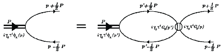
Figure 2: Diagramatic representation of the Bethe Salpeter equation.

As shown in table 1 we obtain the physical pion mass for reasonable values of the current quark mass $m_{0}$.

The model realizes the Goldstone theorem. To see it explicitly we can go to the exact chiral limit, by choosing the reference frame where $P^{\mu}=\left(M,\vec{0}\right)$ and taking the limit $M\rightarrow 0.$ The explicit realization of the Goldstone theorem arises because chiral symmetry implies that we must use the same kernel in the Dyson equation for the mass, equation (II.12), and in the BSE for the pion, equation (III.2) DelbourgoScadron79 . Notice that $G_{p}\left(p\right)$ is not constrained in the procedure.

IV The quark-photon vertex.

In order to study the electromagnetic properties of the pion we describe the coupling of the dressed quarks to the photon. The usual approach to the quark photon vertex is to exploit the Ward-Takahashi Identity (WTI), which is a consequence of gauge invariance in QED. The WTI is satisfied order by order in perturbation theory and must be satisfied also non perturbatively in order to have the right normalization for the quark-photon vertex.

The WTI for the fermion-photon vertex is

$$\left(p_{1}-p_{2}\right)_{\mu}\Gamma^{\mu}\left(p_{1},p_{2}\right)=S^{-1}\left(p_{1}\right)-S^{-1}\left(p_{2}\right)\ .$$ (IV.1)

This equation constrains only the longitudinal component of the proper vertex and therefore provides no information on the transverse part of $\Gamma^{\mu}\left(p_{1},p_{2}\right)$.

Ball and Chiu BallChiu80 have given the form of the most general fermion-photon vertex that satisfies the WTI. It consists of a longitudinally-constrained part given by

$$\Gamma_{BC}^{\mu}\left(p_{1},p_{2}\right) =\frac{1}{2}\left[\frac{1}{Z\left(p_{1}\right)}+\frac{1}{Z\left(p_{2}\right)}\right]\gamma^{\mu}+\frac{1}{2}\left[\frac{1}{Z\left(p_{1}\right)}-\frac{1}{Z\left(p_{2}\right)}\right]\frac{\left(p_{1}+p_{2}\right)^{\mu}}{p_{1}^{2}-p_{2}^{2}}\left(\not p_{1}+\not p_{2}\right)$$

$$-\left[\frac{m\left(p_{1}\right)}{Z\left(p_{1}\right)}-\frac{m\left(p_{2}\right)}{Z\left(p_{2}\right)}\right]\frac{\left(p_{1}+p_{2}\right)^{\mu}}{p_{1}^{2}-p_{2}^{2}}\ \ ,$$ (IV.2)

and a transverse part which is described in term of a basis of eight transverse vectors $T_{i}^{\mu}\left(p_{1},p_{2}\right)$ given in appendix A. The full quark-photon vertex can be written as

$$\Gamma^{\mu}\left(p_{1},p_{2}\right)=\Gamma_{BC}^{\mu}\left(p_{1},p_{2}\right)+\sum_{i=1}^{8}\mathcal{V}_{i}\left(p_{1},p_{2}\right)T_{i}^{\mu}\left(p_{1},p_{2}\right)\ ,$$ (IV.3)

where $\mathcal{V}_{i}\left(p_{1},p_{2}\right)$ are not constrained scalar functions of $p_{1}$ and $p_{2}$ with the correct C, P, T invariance properties.

In our scheme the coupling of photons to quarks arises automatically by implementing gauge invariance in our lagrangian. The usual way to proceed is to introduce path ordered exponentials in the definition of the currents and therefore they become

$$J_{S}\left(x\right) =\int d^{4}y\,G_{0}\left(y\right)\bar{\psi}\left(x+\frac{1}{2}y\right)~{}\mathcal{P}\left(e^{-iQ\int_{x-\frac{1}{2}y}^{x+\frac{1}{2}y}dz^{\mu}A_{\mu}\left(z\right)}\right)~{}\psi\left(x-\frac{1}{2}y\right)\ ,$$ (IV.4)

$$\vec{J}_{5}\left(x\right) =\int d^{4}y\,G_{0}\left(y\right)\bar{\psi}\left(x+\frac{1}{2}y\right)~{}\mathcal{P}\left(e^{-iQ\int_{x}^{x+\frac{1}{2}y}dz^{\mu}A_{\mu}\left(z\right)}\right)~{}i\vec{\tau}\gamma_{5}~{}\mathcal{P}\left(e^{-iQ\int_{x-\frac{1}{2}y}^{x}dz^{\mu}A_{\mu}\left(z\right)}\right)~{}\psi\left(x-\frac{1}{2}y\right)\ ,$$ (IV.5)

$$J_{p}\left(x\right) =\int d^{4}y\,G_{p}\left(y\right)\frac{1}{2}\left[\bar{\psi}\left(x+\frac{1}{2}y\right)~{}\mathcal{P}\left(e^{-iQ\int_{x-\frac{1}{2}y}^{x+\frac{1}{2}y}dz^{\mu}A_{\mu}\left(z\right)}\right)~{}i\ \hbox to0.0pt{$/$\hss}D\ \psi\left(x-\frac{1}{2}y\right)\right.$$

$$~{}~{}~{}~{}~{}~{}~{}~{}~{}~{}~{}~{}~{}~{}~{}~{}~{}~{}~{}~{}-\left.i\bar{\psi}\left(x+\frac{1}{2}y\right)\overleftarrow{\hbox to0.0pt{$/$\hss}D}~{}\mathcal{P}\left(e^{-iQ\int_{x-\frac{1}{2}y}^{x+\frac{1}{2}y}dz^{\mu}A_{\mu}\left(z\right)}\right)~{}\psi\left(x-\frac{1}{2}y\right)\right]\ ,$$ (IV.6)

where the quark charge is $Q=e\left(\vec{\tau}.\hat{n}+1/3\right)/2$ with $\hat{n}=\left(0,0,1\right),$ $\hbox to0.0pt{$/$\hss}D\psi\left(x\right)=\hbox to0.0pt{$/$\hss}\partial\psi\left(x\right)+iQ\hbox to0.0pt{$/$\hss}A\left(x\right)\psi\left(x\right)$ and $\bar{\psi}\left(x\right)\overleftarrow{\hbox to0.0pt{$/$\hss}D}=\partial^{\mu}\bar{\psi}\left(x\right)\gamma_{\mu}-i\bar{\psi}\left(x\right)\hbox to0.0pt{$/$\hss}A\left(x\right)Q.$ In this way $J_{S}$ and $J_{p}$ and $\vec{J}_{5}^{\,2}$ become invariant under local gauge transformations.

The evaluation of the $z_{\mu}$ integrals in Eqs. (IV.4-IV.6) implies a choice of path. The path dependence is implicit in the non locality of the interaction and cannot be avoided. The difference of the contribution between two paths is a gauge invariant quantity which is associated with the magnetic flux through any closed surface defined by the two paths. However, when the photon momentum vanishes the path dependence disappears.

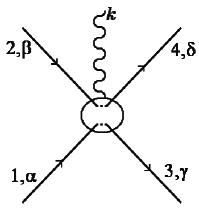
Figure 3: Four quark- photon vertex $\Gamma_{i,\mu}^{(4q\gamma)}\left(p_{1},p_{2};p_{3},p_{4}\right)$ where $i=S,5,p$ recalls the current from which the vertex originates

The quantization of the photon field in Eqs.(IV.4 -IV.6) leads to the new vertex shown in Fig. 3, whose contribution has been fully worked out in Appendix A. The full quark-photon vertex can be constructed in two steps. The first consists in the renormalization of the bare quark-photon vertex by the 4 quarks one photon vertex. Let us call the new vertex, shown in Fig. 4, $\Gamma_{0}^{\mu}\left(p_{1},p_{2}\right)$. Using Eqs.(A.21) and (A.24) of Appendix A we get

$$\Gamma_{0}^{\mu}\left(p_{1},p_{2}\right) =\gamma^{\mu}-\alpha_{0}\left[\left(p_{1}+p_{2}\right)^{\mu}\,\mathbb{V}_{0a}\left(\bar{p},k\right)+k^{\mu}\,\mathbb{V}_{0b}\left(\bar{p},k\right)\right]-$$

$$\alpha_{p}\frac{1}{2}\left[G_{p}\left(p_{1}\right)+G_{p}\left(p_{2}\right)\right]\mathbb{\gamma}^{\mu}-$$

$$\alpha_{p}\frac{\hbox to0.0pt{$/$\hss}p_{1}+\hbox to0.0pt{$/$\hss}p_{2}}{2}\left[\left(p_{1}+p_{2}\right)^{\mu}\,\mathbb{V}_{pa}\left(\bar{p},k\right)+k^{\mu}\,\mathbb{V}_{pb}\left(\bar{p},k\right)\right]$$ (IV.7)

with $k=p_{2}-p_{1},$ $\bar{p}=\frac{p_{1}+p_{2}}{2}$ and $\mathbb{V}_{0a},$ $\mathbb{V}_{0b},$ $\mathbb{V}_{pa}$ and $\mathbb{V}_{pb}$ given in Eqs (A.20) and (A.25) of Appendix A. Both the scalar and momentum currents contribute to this vertex.

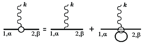
Figure 4: Diagramatic representation of eq. (IV.7).

The second step consists in the insertion of $\Gamma_{0}^{\mu}\left(p_{1},p_{2}\right)$ in the equation for the quark-photon vertex, represented in Fig. 5, which produces the dressed quark-photon vertex,

$$i\Gamma^{\mu}\left(p_{1},p_{2}\right)=i\Gamma_{0}^{\mu}\left(p_{1},p_{2}\right)+i2g_{0}G_{0}\left(\frac{p_{1}+p_{2}}{2}\right)\int\frac{d^{4}p}{\left(2\pi\right)^{4}}G_{0}\left(p\right)\,\mathbb{T}\text{r}\left[i\,S\left(p-\frac{k}{2}\right)\,i\,S\left(p+\frac{k}{2}\right)i\Gamma^{\mu}\left(p-\frac{k}{2},p+\frac{k}{2}\right)\right]$$

$$+i2g_{p}~{}\left(\frac{\hbox to0.0pt{$/$\hss}p_{1}+\hbox to0.0pt{$/$\hss}p_{2}}{2}\right)~{}G_{p}\left(\frac{p_{1}+p_{2}}{2}\right)\int\frac{d^{4}p}{\left(2\pi\right)^{4}}G_{p}\left(p\right)\,\mathbb{T}\text{r}\left[i\,S\left(p-\frac{k}{2}\right)\hbox to0.0pt{$/$\hss}p\,i\,S\left(p+\frac{k}{2}\right)i\Gamma^{\mu}\left(p-\frac{k}{2},p+\frac{k}{2}\right)\right]~{}~{}.$$ (IV.8)

It is easy to show that the solution of equation (IV.8) is just

$$\Gamma^{\mu}\left(p_{1},p_{2}\right)=\Gamma_{0}^{\mu}\left(p_{1},p_{2}\right)~{}~{}.$$ (IV.9)

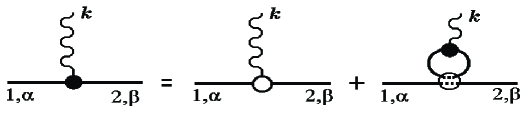
Figure 5: Diagramatic representation of eq. (IV.8).

In agreement with our previous discussion, the quark-photon vertex can be rewritten in the form given by equation (IV.3),

$$\Gamma^{\mu}\left(p_{1},p_{2}\right)=\Gamma_{BC}^{\mu}\left(p_{1},p_{2}\right)+\mathcal{V}_{1}\left(p_{1},p_{2}\right)T_{1}^{\mu}\left(p_{1},p_{2}\right)+\mathcal{V}_{2}\left(p_{1},p_{2}\right)T_{2}^{\mu}\left(p_{1},p_{2}\right)\ ,$$ (IV.10)

where

$$\mathcal{V}_{1}\left(p_{1},p_{2}\right) =\frac{2\alpha_{0}}{p_{2}^{2}-p_{1}^{2}}\mathbb{V}_{0b}\left(\bar{p},k\right)\ ,$$ (IV.11)

$$\mathcal{V}_{2}\left(p_{1},p_{2}\right) =\frac{2\alpha_{p}}{p_{2}^{2}-p_{1}^{2}}\mathbb{V}_{pb}\left(\bar{p},k\right)\ .$$ (IV.12)

In summary, we have constructed a dressed quark-photon vertex which has all the desired properties. It is gauge invariant in the local sense, without being obtained from the WTI. Two new terms appear from the restoration of the local gauge symmetry. The simplest expressions for these terms can be built assuming that a straight line joins the two points characterizing the non local currents. For that simple input we obtain

$$\mathcal{V}_{1}\left(p_{1},p_{2}\right) =\frac{1}{p_{2}^{2}-p_{1}^{2}}\int_{-1}^{1}d\lambda\;\lambda\;\left[\frac{d}{dp^{2}}\frac{m\left(p\right)}{Z\left(p\right)}\right]_{p^{2}=\left(\bar{p}-\frac{\lambda}{2}k\right)^{2}}\ ,$$ (IV.13)

$$\mathcal{V}_{2}\left(p_{1},p_{2}\right) =\frac{-1}{p_{2}^{2}-p_{1}^{2}}\int_{-1}^{1}d\lambda\;\lambda\;\left[\frac{d}{dp^{2}}\frac{1}{Z\left(p\right)}\right]_{p^{2}=\left(\bar{p}-\frac{\lambda}{2}k\right)^{2}}\ ,$$ (IV.14)

which can be directly evaluated from the form of the quark propagator.

V The axial current and $f_{\pi}$.

Lets us now turn to the coupling of the axial current to quarks. The WTI in this case is

$$\left(p_{2}-p_{1}\right)_{\mu}\Gamma_{5}^{\mu}\left(p_{1},p_{2}\right)\tau^{i}=S^{-1}\left(p_{2}\right)\gamma_{5}\tau^{i}+\gamma_{5}\tau^{i}S^{-1}\left(p_{1}\right)-2m_{0}i~{}\Gamma_{5}\left(p_{1},p_{2}\right)\tau^{i}\ .$$ (V.1)

The last term, proportional to $m_{0},$ disappears in the chiral limit.

Our first step is to obtain $\Gamma_{5}\left(p_{1},p_{2}\right)\tau^{i},$ which corresponds to the dressing of the vertex $i\gamma_{5}\tau^{i}.$ Now the external probe is a pseudoscalar-isovector therefore we will have contribution from the pseudoscalar current, $\vec{J}_{5},$

$$\Gamma_{5}\left(p_{1},p_{2}\right)\tau^{i}=i\gamma_{5}\tau^{i}+i2g_{0}G_{0}\left(\bar{p}\right)\,i\gamma_{5}\tau^{j}\,$$

$$\int\frac{d^{4}p}{\left(2\pi\right)^{4}}G_{0}\left(p\right)\,\left(-\right)\mathbb{T}\text{r}\left[i\,S\left(p-\frac{k}{2}\right)\,i\gamma_{5}\tau^{j}\,i\,S\left(p+\frac{k}{2}\right)\Gamma_{5}\left(p-\frac{k}{2},p+\frac{k}{2}\right)\tau^{i}\right]~{}~{}.$$ (V.2)

with $p_{1}=\bar{p}-\frac{k}{2}$ and $p_{2}=\bar{p}+\frac{k}{2}.$ This equation can be easily solved obtaining

$$\Gamma_{5}\left(p_{1},p_{2}\right)=i\gamma_{5}\left[1+2g_{0}~{}G_{0}\left(\bar{p}\right)\frac{F_{0}\left(k^{2}\right)}{1-2g_{0}~{}\Pi_{PS}\left(k^{2}\right)}\right]$$ (V.3)

where $F_{0}\left(k^{2}\right)$ is defined by

$$\delta^{ij}F_{0}\left(k^{2}\right)=-i\int\frac{d^{4}p}{\left(2\pi\right)^{4}}G_{0}\left(p\right)\,\mathbb{T}\text{r}\left(i\,\gamma_{5}\tau^{i}i\,S\left(p-\frac{1}{2}k\right)\,i\,\gamma_{5}\tau^{j}i\,S\left(p+\frac{1}{2}k\right)\right)~{}~{}.$$ (V.4)

We will obtain the dressed vertex $\Gamma_{5}^{\mu}\left(p_{1},p_{2}\right)$ applying to the $W^{\pm}$ bosons the same procedure developed for photons in the previous section. The explicit calculation is given in Appendix B. The final result, given in equation (B.39), can be rewritten in the following way:

$$\Gamma_{5}^{\mu}\left(p_{1},p_{2}\right) =\tilde{\Gamma}_{5}^{\mu}\left(p_{1},p_{2}\right)$$

$$+\mathcal{A}_{1}\left(p_{1},p_{2}\right)T_{1}^{\mu}\left(p_{1},p_{2}\right)\gamma_{5}+\mathcal{V}_{2}\left(p_{1},p_{2}\right)T_{2}^{\mu}\left(p_{1},p_{2}\right)\gamma_{5}~{}~{},$$ (V.5)

where

$$\mathcal{A}_{1}\left(p_{1},p_{2}\right)=\frac{2\alpha_{0}}{p_{2}^{2}-p_{1}^{2}}\left[\frac{2G_{0}\left(\bar{p}\right)-G_{0}\left(p_{1}\right)-G_{0}\left(p_{2}\right)}{\left(p_{1}-p_{2}\right)^{2}}+\mathbb{A}_{0b}\left(\bar{p},k\right)\right]\ ,$$ (V.6)

with $\mathbb{A}_{0b}\left(\bar{p},k\right)$ given in eq (A.23b), and

$$\tilde{\Gamma}_{5}^{\mu}\left(p_{1},p_{2}\right) =\frac{1}{2}\left[\frac{1}{Z\left(p_{1}\right)}+\frac{1}{Z\left(p_{2}\right)}\right]\gamma^{\mu}\gamma_{5}+\frac{1}{2}\left[\frac{1}{Z\left(p_{2}\right)}-\frac{1}{Z\left(p_{1}\right)}\right]\frac{\left(p_{1}+p_{2}\right)^{\mu}}{p_{2}^{2}-p_{1}^{2}}\left(\not p_{1}+\not p_{2}\right)\gamma_{5}$$

$$-\left[\frac{m\left(p_{1}\right)}{Z\left(p_{1}\right)}+\frac{m\left(p_{2}\right)}{Z\left(p_{2}\right)}\right]\frac{\left(p_{2}-p_{1}\right)^{\mu}}{\left(p_{2}-p_{1}\right)^{2}}\gamma_{5}-i2m_{0}\Gamma_{5}\left(p_{1},p_{2}\right)\frac{\left(p_{2}-p_{1}\right)^{\mu}}{\left(p_{2}-p_{1}\right)^{2}},$$ (V.7)

is the longitudinally constrained part of $\Gamma_{5}^{\mu}\left(p_{1},p_{2}\right).$

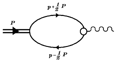
Figure 6: Diagramatic representation of the pion decay process corresponding to eq. (V.8).

Let us now to look for the pion decay constant. In this calculation only the longitudinal current is needed and so we do not need to choose a particular path. There are several equivalent ways for obtaining the pion decay constant, depending where the quark-quark interaction is included. The simplest one is through the diagram depicted in figure 6, in which all the $q\bar{q}$ bubbles are included in the Bethe-Salpeter pion amplitude. The axial vertex includes those vertex corrections which can not be included in the bound state amplitude, which in our case corresponds to those depicted in Fig 4. Therefore, the pion decay constant is defined by,

$$i~{}\delta_{i,j}~{}f_{\pi}~{}P^{\mu}=$$

$$\int\frac{d^{4}p}{\left(2\pi\right)^{4}}\left(-\right)\mathbb{T}\text{r}\left[i\,\phi_{\pi}\left(p,P\right)\ i\gamma_{5}\ \tau^{i}\ i\ S\left(p-\frac{1}{2}P\right)\ \Gamma_{5,0}^{\mu}\left(p+\frac{1}{2}P,p-\frac{1}{2}P\right)\ \frac{\tau^{j}}{2}\ i\ S\left(p+\frac{1}{2}P\right)\right]~{},$$ (V.8)

where $\Gamma_{5,0}^{\mu}\left(p_{1},p_{2}\right)$ is given in equation (B.36) of Appendix B and $\phi_{\pi}\left(p,P\right)$ given by equation (III.3). A direct calculation gives the result,

$$f_{\pi}=\frac{g_{\pi qq}}{P^{2}}\left\{\frac{1}{2}\left(1-2g_{0}\Pi_{PS}\left(P^{2}\right)\right)F_{1}\left(P^{2}\right)+m_{0}F_{0}\left(P^{2}\right)\right\}~{}~{}.$$ (V.9)

with $F_{0}$ given in equation (V.4) and

$$F_{1}\left(P^{2}\right)=-\int\frac{d^{4}p}{\left(2\pi\right)^{4}}\left(G_{0}\left(p+\frac{P}{2}\right)+G_{0}\left(p-\frac{P}{2}\right)\right)\mathbb{T}\text{r}\left[i\,S\left(p\right)\right]~{}.$$ (V.10)

We have two clearly distinguishable situations. In the chiral limit $f_{\pi}$ is determined by the term with $F_{1}\left(P^{2}\right)$. In this limit, $F_{1}\left(0\right)$ is the integral evaluated in equation (II.12). Using in the latter equations (III.5) and (III.6) and substituting, we obtain

$$f_{\pi}=\frac{\alpha_{0}}{g_{\pi qq}}=\frac{m\left(0\right)}{g_{\pi qq}Z\left(0\right)}~{}.$$ (V.11)

The last form of $f_{\pi}$ is the Goldberger-Treiman relation. The crucial point for obtaining this result is the chiral symmetric structure of the interaction, which connects the kernel present in the calculation of $f_{\pi}$, associated with the pseudoscalar-isovector current present in our lagrangian, with the one present in the evaluation of the mass term $m\left(0\right),$ associated to the scalar-isoscalar current.

If we work with physical pions ($m_{0}\neq 0),$ the pion decay constant is given by

$$f_{\pi}=\frac{m_{0}}{m_{\pi}^{2}}g_{\pi qq}F_{0}\left(m_{\pi}^{2}\right)~{}.$$ (V.12)

In this case the surviving contribution arises from the pion pole present in $\Gamma_{5}\left(p_{1},p_{2}\right)$.

Using equations (V.4), (II.15) and (II.26) we can obtain approximative expressions for $F_{0}\left(m_{\pi}^{2}\right)$ which lead directly to the Gell-Mann-Oakes-Renner relation

$$f_{\pi}^{2}=-N_{f}~{}\left\langle\bar{q}q\right\rangle\frac{m_{0}}{m_{\pi}^{2}}+\mathcal{O}\left(m_{0},m_{\pi}^{2}\right)~{}.$$ (V.13)

We have seen that we have different expressions for $f_{\pi}$ in the chiral limit and in the physical case. They originate from different terms of the axial current. Nevertheless, chiral symmetry guarantees that (V.11) is the limit of equation (V.12) when $m_{0}$ goes to zero.

In table 1 we give numerical values for $f_{\pi}$ for scenarios S1 and S2 previously discussed. They are in reasonably good agreement with the experimental results. Moreover, this two scenarios are describing the same physics, even if they have a very different origin.

From reference MarisRobertsTandy98 we can infer that the pion decay constant is determined using equation (V.8) with the approximated expression for the axial vertex,

$$\Gamma_{5}^{\prime\mu}\left(p_{1},p_{2}\right)=\frac{1}{2}\left[\frac{1}{Z\left(p_{1}\right)}+\frac{1}{Z\left(p_{2}\right)}\right]\gamma^{\mu}\gamma_{5}+\frac{1}{2}\left[\frac{1}{Z\left(p_{1}\right)}-\frac{1}{Z\left(p_{2}\right)}\right]\frac{\left(p_{1}+p_{2}\right)^{\mu}}{p_{1}^{2}-p_{2}^{2}}\left(\hbox to0.0pt{$/$\hss}p_{1}+\hbox to0.0pt{$/$\hss}p_{2}\right)\gamma_{5}+\mathcal{O}\left(p_{1}-p_{2}\right)\ .$$ (V.14)

In this expression $\mathcal{O}\left(p_{1}-p_{2}\right)$ implies that $\left(p_{1}-p_{2}\right)_{\mu}\Gamma_{5}^{\prime\mu}\left(p_{1},p_{2}\right)$ is determined up to terms of order $\left(p_{1}-p_{2}\right)^{2}=P^{2}.$ This expression is the minimal generalization of the bare $\gamma^{\mu}\gamma_{5}$ vertex in the case where $Z\left(p\right)\neq 1.$ It is straightforward to proof that the $f_{\pi}$ obtained in this way differs from the exact one by corrections of order $m_{\pi}^{2}$. Therefore, equation (V.14) gives the right result in the chiral limit and a good approximation to the exact value in the physical case. The Gell-Mann-Oakes-Renner relation is also well reproduced in this approximation. Nevertheless, equation (V.14) is not a good expression for the axial vertex, for instance the pion pole is not present in this expression. So we conclude that $\Gamma_{5}^{\prime\mu}\left(p_{1},p_{2}\right)$ is a good approximation of the longitudinal part of $\Gamma_{5,0}^{\mu}\left(p_{1},p_{2}\right)$ in the vicinity of the pion mass ($P^{2}\sim m_{\pi}^{2})$, as it can be see from equation (B.40).

Let us now consider the coupling of the axial current to a line of quarks through the vertex, $\Gamma_{5}^{\mu}\left(p_{1},p_{2}\right).$ This coupling contains the direct coupling and the pion pole contribution. We observe from equations (V.7) and (V.3) that the pion pole contribution goes trough the $\Gamma_{5}\left(p_{1},p_{2}\right)$ term when the chiral symmetry is explicitly broken. In the chiral limit, the pion pole is present in the term with quark masses in $\tilde{\Gamma}_{5}^{\mu}\left(p_{1},p_{2}\right)$. The full $\Gamma_{5}^{\mu}\left(p_{1},p_{2}\right)$ has some dependence on the choice of path. Nevertheless, the overall procedure preserves all the symmetries and, in particular, gauge symmetry.

The longitudinal part of the axial current, $\tilde{\Gamma}_{5}^{\mu}\left(p_{1},p_{2}\right),$ is path independent. Using equations (V.12) and (V.13), and assuming that $P^{2}\lesssim m_{\pi}^{2},$ it can be written in terms of the pion wave function as

$$\tilde{\Gamma}_{5}^{\mu}\left(p_{1},p_{2}\right)\frac{\tau^{i}}{2} =\frac{1}{2}\left[\frac{1}{Z\left(p_{1}\right)}+\frac{1}{Z\left(p_{2}\right)}\right]\gamma^{\mu}\gamma_{5}\frac{\tau^{i}}{2}+\frac{1}{2}\left[\frac{1}{Z\left(p_{2}\right)}-\frac{1}{Z\left(p_{1}\right)}\right]\frac{\left(p_{1}+p_{2}\right)^{\mu}}{p_{2}^{2}-p_{1}^{2}}\left(\not p_{1}+\not p_{2}\right)\gamma_{5}\frac{\tau^{i}}{2}$$

$$-\left[\frac{m\left(p_{1}\right)}{Z\left(p_{1}\right)}+\frac{m\left(p_{2}\right)}{Z\left(p_{2}\right)}\right]\frac{\left(p_{2}-p_{1}\right)^{\mu}}{\left(p_{2}-p_{1}\right)^{2}}\gamma_{5}\frac{\tau^{i}}{2}+$$

$$\left(m_{0}+m_{\pi}^{2}f_{\pi}\frac{\phi_{\pi}\left(p\right)}{P^{2}-m_{\pi}^{2}}\right)\gamma_{5}\tau^{i}\frac{\left(p_{2}-p_{1}\right)^{\mu}}{\left(p_{2}-p_{1}\right)^{2}},$$ (V.15)

with $p_{1,2}=p\pm\frac{1}{2}P.$ Equation (V.15) manifests the pion pole explicitly, as is predicted by PCAC.

VI Electromagnetic Pion form factor.

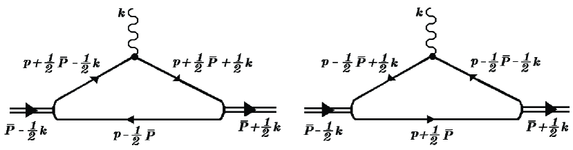
Figure 7: Triangle diagram contributing to the pion form factor.

We begin by considering the triangle diagram of Fig. 7. In order to fix ideas let us consider the interaction of a photon with a $\pi^{+}$. With the momenta defined as in the figure we have

$$i\,e\,2\,\bar{P}^{\mu}F^{\left(2q\gamma\right)}\left(k^{2}\right)=\int\frac{d^{4}p}{\left(2\pi\right)^{4}}\left(-\right)\,\mathbb{T}\text{r}\left[i\,\gamma_{5}\,\tau^{+}\phi_{\pi}\left(p-\frac{1}{4}k\right)i\,S\left(p-\frac{1}{2}\bar{P}\right)\right.$$

$$\left.\,i\,\gamma_{5}\,\left(\tau^{+}\right)^{{\dagger}}\,\phi_{\pi}\left(p+\frac{1}{4}k\right)\,i\,S\left(p+\frac{1}{2}\bar{P}+\frac{1}{2}k\right)\,iQ\,\Gamma^{\mu}\left(p+\frac{1}{2}\bar{P}-\frac{1}{2}k,p+\frac{1}{2}\bar{P}+\frac{1}{2}k\right)\,i\,S\left(p+\frac{1}{2}\bar{P}-\frac{1}{2}k\right)\right]$$

$$+\int\frac{d^{4}p}{\left(2\pi\right)^{4}}\left(-\right)\,\mathbb{T}\text{r}\left[i\,\gamma_{5}\,\tau^{+}\,\phi_{\pi}\left(p+\frac{1}{4}k\right)\,i\,S\left(p-\frac{1}{2}\bar{P}+\frac{1}{2}k\right)\,i\,Q\,\Gamma^{\mu}\left(p-\frac{1}{2}\bar{P}-\frac{1}{2}k,p-\frac{1}{2}\bar{P}+\frac{1}{2}k\right)\right.$$

$$\left.i\,S\left(p-\frac{1}{2}\bar{P}-\frac{1}{2}k\right)\,i\,\gamma_{5}\,\left(\tau^{+}\right)^{{\dagger}}\,\phi_{\pi}\left(p-\frac{1}{4}k\right)\,i\,S\left(p+\frac{1}{2}\bar{P}\right)\right]\ \ ,$$ (VI.1)

where $\phi_{\pi}$ is the pion Bethe-Salpeter amplitude given in equation (III.3) and $\Gamma^{\mu}\left(p_{1},p_{2}\right)$ is the dressed quark-photon coupling given in equation (IV.10).

There is another contribution to the form factor to be added to the previous one. The $\vec{J}_{5}^{\,2}\left(x\right)$ term produces a four quark photon vertex evaluated in Appendix A and given by equation (A.22). This four quark photon vertex allows for an additional diagram shown in Fig. 8. This contribution is

$$i\,e\,2\,\bar{P}_{\mu}F^{(4q\gamma)}\left(k^{2}\right)=-\int\frac{d^{4}p}{\left(2\pi\right)^{4}}\int\frac{d^{4}p^{\prime}}{\left(2\pi\right)^{4}}\,\left[i\,S\left(p^{\prime}-\frac{1}{2}P^{\prime}\right)i\,\gamma_{5}\,\left(\tau^{+}\right)^{{\dagger}}\,\phi_{\pi}\left(p^{\prime}\right)i\,S\left(p^{\prime}+\frac{1}{2}P^{\prime}\right)\right]_{\alpha\gamma}$$

$$\,\left[\,\Gamma_{5,\mu}^{(4q\gamma)}\left(p^{\prime}-\frac{1}{2}P^{\prime},p^{\prime}+\frac{1}{2}P^{\prime};p+\frac{1}{2}P,p-\frac{1}{2}P\right)\right]_{\alpha\beta,\gamma\delta}\,\left[i\,S\left(p+\frac{1}{2}P\right)i\,\gamma_{5}\,\tau^{+}\phi_{\pi}\left(p\right)i\,S\left(p-\frac{1}{2}P\right)\right]_{\beta\delta}.$$ (VI.2)

Therefore, the full electromagnetic form factor is $F\left(k^{2}\right)=F^{\left(2q\gamma\right)}\left(k^{2}\right)+F^{\left(4q\gamma\right)}\left(k^{2}\right)$.

Global gauge invariance guarantees the right normalization for the form factor, $F\left(k^{2}=0\right)=1$. For a general case, the right normalization of the form factor is assured by the Ward identity, equation (IV.1), provided that $\phi_{\pi}$ is normalized by equation (III.6) and we take into account the two contributions arising from Eqs. (VI.1) and (VI.2). When the kernel used in the pion BSE, equation (III.5), is independent on the total pion momentum, as it is for our models, the contribution arising from the triangle diagram, equation (VI.1) will assure the correct normalization of the form factor. Therefore, in our case this property is guaranteed for the full $\Gamma^{\mu}\left(p_{1},p_{2}\right)$ vertex given by equation (IV.10) and for the Ball-Chiu vertex, $\Gamma_{BC}^{\mu}\left(p_{1},p_{2}\right),$ given by equation (IV.2). In our expression for $\Gamma^{\mu}\left(p_{1},p_{2}\right)$ there are additional terms besides $\Gamma_{BC}^{\mu}\left(p_{1},p_{2}\right)$ which arise from local gauge invariance. They give contributions to $F\left(k^{2}\right)$ for $k^{2}\neq 0$ without modifying the value at $k^{2}=0.$

Due to the separable nature in $p$ and $p^{\prime}$ and $P$ -independence of the interacting terms in our Lagrangian, one of the integrals in equation (VI.2) can be done in a trivial manner generating a pion-2 quark-photon vertex. However, when performing the remaining integrals we realize that this diagram does not contribute to the form factor. This is not a general result, just a consequence of our particular models. In fact this term will contribute in a significant way to the parton distribution NogueraVento05 . Its contribution is crucial to guarantee isospin symmetry in the parton distributions and to restore the momentum sum rule.

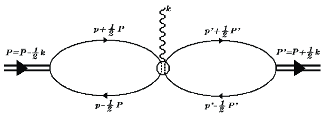
Figure 8: Contribution to the form factor coming from the four quark-photon vertex displayed in Fig. 3

We now proceed to a numerical comparison between the calculations, using the Ball-Chiu vertex, and our full locally gauge invariant vertex, equation (IV.10), (IV.13) and (IV.14). We show in Fig. 9 the form factor for the two vertices in scenarios S1 and S2, together with the experimental results Bebek76 ; Amendola86 . We find no important differences for S1 when comparing the Ball-Chiu prescription to the full vertex. For S2 the correction, which is small for small $k^{2},$ becomes important for $k^{2}\sim-0.8\operatorname{GeV}^{2}$. The difference in the calculations arises because in S2 $Z\left(p\right)\neq 1$. The correction due to $\mathcal{V}_{1}\left(p_{1},p_{2}\right)$ is about 5-7% at this momentum transfer for both scenarios. The correction due to $\mathcal{V}_{2}\left(p_{1},p_{2}\right)$, present only in S2, is about 24% for $k^{2}\sim-0.8\operatorname{GeV}^{2}$. Since the two corrections go in the same direction the overall result changes by about 30%. We have confirmed this conclusion introducing a $Z\left(p\right)$ different from 1 in case S1.

Regarding the experimental results we observe that the scenario S1 reproduces well the value of $F\left(k^{2}\right)$ for small values of $k$ but underestimates the form factor for $k^{2}\sim 0.8\operatorname{GeV}^{2}$ by as much as 12%. For scenario S2 we observe that the introduction of the full vertex produces a better description of the form factor for $k^{2}\sim 0.8\operatorname{GeV}^{2}$ but a worst in the small $k$ region. In this last scenario the difference between the calculated form factor and the experimental data is always less than 5%.

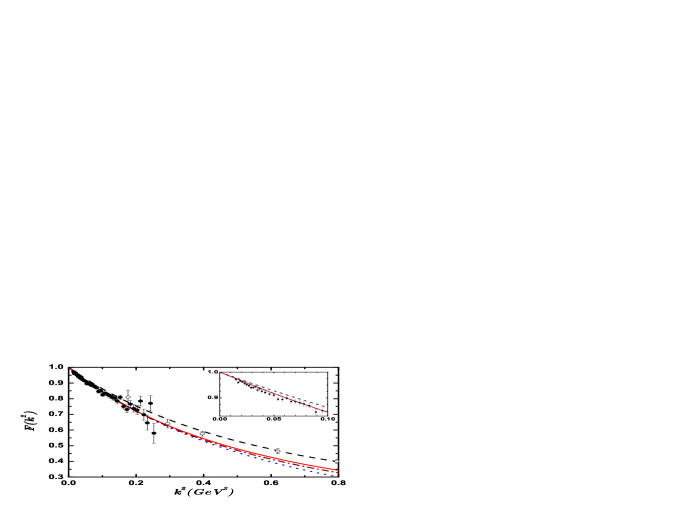
Figure 9: Comparison of the Pion form factor calculated in the two defined scenarios with the Ball-Chiu ansatz and the full vertex of the model. Dot-dashed curve corresponds to the scenario S1 with Ball-Chiu ansatz; full curve corresponds to the same scenario with the full vertex. Dotted curve corresponds to S2 with the Ball-Chiu ansatz; dashed curve corresponds to S2 with the full vertex. Experimental data have been taken from Amendola86 (points) and from Bebek76 (circles).

The behavior for small $k$ can be analyzed in terms of the pion radius. In table 1 we give the mean squared radius for the full electromagnetic vertex and, between brackets, that of the Ball-Chiu prescription. We observe that the radius is smaller than the experimental result in all cases. We also observe that the full vertex and the Ball-Chiu prescription produce the same values since there is no wave function renormalization in the quark propagator, as in the case S1. In model S2, with non vanishing wave function renormalization, we observe a difference, of about 15%, due to the $\mathcal{V}_{2}\left(p_{1},p_{2}\right)$ term in equation (IV.10), confirming our conclusion from the analysis of the form factors. Summarizing, the use of the full vertex increases the differences between the calculation and the observation. But this is not unexpected since no vector mesons have been included in the models and previous work indicates that this contribution can be of the order of 10-20% MarisTandi00 ; Dorokhov3 ; OconnellPearceThomasWilliams97 .

We analyze the dependence of the pion radius in $m\left(p\right)$ and $Z\left(p\right)$ in the chiral limit ($m_{0}=0).$ In Fig. 10 we show the result of rescaling by a generic factor of $\lambda$ the parameters $\Lambda_{m}$ and $\alpha_{m}$ appearing in Eqs.(II.24) and (II.25). If $\Lambda_{m}$ increases the interaction $\vec{J}_{5}^{\,2}\left(x\right)$ becomes of shorter range. If we increase $\alpha_{m},$ $g_{0}$ increases. In both cases the pion becomes more bound and its radius smaller.

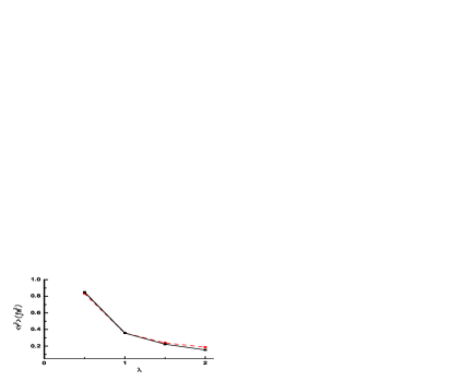
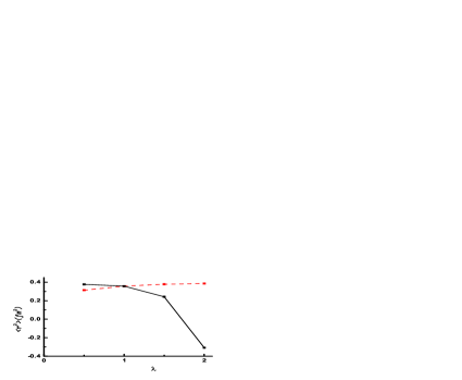
Figure 10: Sensitivity of $\left\langle r^{2}\right\rangle$ in $\operatorname{fm}^{2}$ for the pion in relation with the propagator parameters in the scenario S2. On the left we have $\left\langle r^{2}\right\rangle$ in relation with $\lambda\cdot\Lambda_{m}$ for $\lambda=0.5,1,1.5$ and $2$ (dashed curve) and $\left\langle r^{2}\right\rangle$ in relation with $\lambda\cdot\alpha_{m}$ for the same values of $\lambda$ (full curve). On the right, the dotted curve represents the $\left\langle r^{2}\right\rangle$ in relation with $\lambda\cdot\Lambda_{z}$  and the full curve gives the $\left\langle r^{2}\right\rangle$ for the pion in relation with $\lambda\cdot\alpha_{z}$, for $\lambda=0.5,1,1.5$ and $2.$ The full curve gives the msr in $\operatorname{fm}^{2}$ for the pion in relation with $\lambda\cdot\alpha_{z}$ for the same values of $\lambda.$

In Fig. 10 we also show what happens to the mean square radius when $\Lambda_{z}$ and $\alpha_{z}$ are rescaled by a factor of $\lambda$. The system is not very sensitive to changes of $\Lambda_{z},$ while it is quite sensitive for the rescaling of $\alpha_{z}$ when $\lambda\sim 2.$ The reason for this strong effect is that for this value $Z\left(0\right)=0.$

VII Parton distribution.

In the previous section we have analyzed some numerical aspects of the pion form factor. We have put special emphasis in the discussion of the terms restoring the local gauge symmetry, $\mathcal{V}_{1}\left(p_{1},p_{2}\right)$ and $\mathcal{V}_{2}\left(p_{1},p_{2}\right)$. We have seen that we have a second contribution given in equation (VI.2), but this contribution vanishes in our particular model. Searching for an observable which is sensible to this term, we next discuss the parton distribution. As it is shown in NogueraTheusslVento04 the operator for the parton distribution can be connected to the electromagnetic operator at zero momentum transfer. Therefore we are dealing with a property for $k^{2}=0,$ where the path dependence is absent and our results will be valid for any model.

The first step is to obtain the electromagnetic operator at zero momentum transfer. This operator has a one body term which can be obtained directly from Ward identity

$$\Gamma^{\mu}\left(p,p\right)=\frac{\partial S^{-1}\left(p\right)}{\partial p_{\mu}}\ ,$$ (VII.1)

and a two body term which corresponds in our particular lagrangian to the equation (VI.2). To be precise, let us proceed to a general discussion. We start from an action of the form

$$S=\int d^{4}x\bar{\psi}\left(x\right)\left(i\not\partial-m_{0}\right)\psi\left(x\right)+$$

$$\int d^{4}x_{1}~{}d^{4}x_{2}~{}d^{4}x_{3}~{}d^{4}x_{4}\,G_{\alpha\beta\gamma\delta}\left(x_{1},x_{2},x_{3},x_{4}\right)\bar{\psi}_{\delta}\left(x_{4}\right)\psi_{\beta}\left(x_{2}\right)\bar{\psi}_{\gamma}\left(x_{3}\right)\psi_{\alpha}\left(x_{1}\right),$$ (VII.2)

where the greek indices characterize all symmetries, i.e spinor, color and flavor. Let us define the following variables,

$$x =\left(x_{3}-x_{1}\right)\ ,\qquad x^{\prime}=\left(x_{4}-x_{2}\right)\ ,$$

$$X^{\prime} =\frac{1}{2}\left(x_{3}+x_{1}-x_{4}-x_{2}\right)\ ,\qquad X=\frac{1}{4}\left(x_{3}+x_{1}+x_{4}+x_{2}\right)\ .$$ (VII.3)

Translational invariance imposes that $G_{\alpha\beta\gamma\delta}\left(x_{1},x_{2},x_{3},x_{4}\right)$ cannot depend on $X.$ We introduce

$$G_{\alpha\beta\gamma\delta}\left(x_{1},x_{2},x_{3},x_{4}\right)=G_{\alpha\beta\gamma\delta}\left(x,x^{\prime},X^{\prime}\right)=\int\frac{d^{4}p}{\left(2\pi\right)^{4}}\frac{d^{4}p^{\prime}}{\left(2\pi\right)^{4}}\frac{d^{4}P}{\left(2\pi\right)^{4}}e^{-ixp}e^{-ix^{\prime}p^{\prime}}e^{-iX^{\prime}P}G_{\alpha\beta\gamma\delta}\left(p,p^{\prime},P\right)\ .$$ (VII.4)

Hermiticity and all internal symmetries, such as parity, charge conjugation and time reversal, impose relations between the different components of the interaction term $G_{\alpha\beta\gamma\delta}\left(p,p^{\prime},P\right).$

We are interested in the mesonic bound state described in Fig. 2. The Bethe-Salpeter amplitude for this meson is defined by (we identify $p_{2}=p^{\prime}+P/2,$ $p_{4}=p^{\prime}-P/2,$ $p_{3}=p+P/2,$ $p_{1}=p-P/2)\$

$$\Gamma_{\gamma\alpha}^{M}\left(p,P\right)=-2i\int\frac{d^{4}p^{\prime}}{\left(2\pi\right)^{4}}G_{\alpha\beta\gamma\delta}\left(p,p^{\prime},P\right)\left(i\,S\left(p^{\prime}+\frac{1}{2}P\right)~{}\Gamma^{M}\left(p^{\prime},P\right)\,i\,S\left(p^{\prime}-\frac{1}{2}P\right)\right)_{\beta\delta}\ \ ,$$ (VII.5)

with the standard normalization condition given in the Appendix C, equation (C.44).

Regarding the charges of the fields in equation (VII.2), we can assume that $Q_{\alpha}=Q_{\delta}=Q_{1}$ and $Q_{\gamma}=Q_{\beta}=Q_{2}.$ We observe that the interaction term in equation (VII.2) is invariant under global gauge transformations but not under local gauge transformations. One way to make it locally invariant is by incorporating some links. The interaction term becomes,

$$S_{i}=\int d^{4}x~{}d^{4}x^{\prime}~{}d^{4}X^{\prime}~{}d^{4}X\,G_{\alpha\beta\gamma\delta}\left(x,x^{\prime},X^{\prime}\right)\bar{\psi}_{\delta}\left(\frac{1}{2}x^{\prime}-\frac{1}{2}X^{\prime}+X\right)e^{-iQ_{1}\int_{X}^{\frac{1}{2}x^{\prime}-\frac{1}{2}X^{\prime}+X}dz^{\mu}A_{\mu}\left(z\right)}$$

$$e^{-iQ_{2}\int_{-\frac{1}{2}x^{\prime}-\frac{1}{2}X^{\prime}+X}^{X}dz^{\mu}A_{\mu}\left(z\right)}\psi_{\beta}\left(-\frac{1}{2}x^{\prime}-\frac{1}{2}X^{\prime}+X\right)\bar{\psi}_{\gamma}\left(\frac{1}{2}x+\frac{1}{2}X^{\prime}+X\right)e^{-iQ_{2}\int_{X}^{\frac{1}{2}x+\frac{1}{2}X^{\prime}+X}dz^{\mu}A_{\mu}\left(z\right)}$$

$$e^{-iQ_{1}\int_{-\frac{1}{2}x+\frac{1}{2}X^{\prime}+X}^{X}dz^{\mu}A_{\mu}\left(z\right)}\psi_{\alpha}\left(-\frac{1}{2}x+\frac{1}{2}X^{\prime}+X\right)\ .$$ (VII.6)

We now expand this expression in powers of the photon field. The first term is already included in equation (VII.2). The second term is linear in the photon field and is the one of interest. We can evaluate it in the $k\rightarrow 0$ limit without having to define a specific path for the integrals present in equation (VII.6). From this last result it is easy to obtain that the quantity to add in the limit of $k\rightarrow 0$ to each vertex of the type of Fig. 3 is

$$-iQ_{1}\left[\Gamma_{1,\mu}^{(4q\gamma)}\left(p_{1},p_{3};p_{2},p_{4}\right)\right]_{\alpha\beta,\gamma\delta}-iQ_{2}\left[\Gamma_{2,\mu}^{(4q\gamma)}\left(p_{1},p_{3};p_{2},p_{4}\right)\right]_{\alpha\beta,\gamma\delta}\ ,$$ (VII.7)

with

$$\left[\Gamma_{1,\mu}^{(4q\gamma)}\left(p_{1},p_{3};p_{2},p_{4}\right)\right]_{\alpha\beta,\gamma\delta}=2\left(\frac{d}{dp_{1}^{\mu}}+\frac{d}{dp_{4}^{\mu}}\right)G_{\alpha\beta\gamma\delta}\left(\frac{p_{1}+p_{3}}{2},\frac{p_{2}+p_{4}}{2},\frac{p_{2}+p_{3}-p_{1}-p_{4}}{2}\right)~{}~{},$$

$$\left[\Gamma_{2,\mu}^{(4q\gamma)}\left(p_{1},p_{3};p_{2},p_{4}\right)\right]_{\alpha\beta,\gamma\delta}=2\left(\frac{d}{dp_{2}^{\mu}}+\frac{d}{dp_{3}^{\mu}}\right)G_{\alpha\beta\gamma\delta}\left(\frac{p_{1}+p_{3}}{2},\frac{p_{2}+p_{4}}{2},\frac{p_{2}+p_{3}-p_{1}-p_{4}}{2}\right)~{}~{}.$$ (VII.8)

The details of the calculation are given in Appendix C, where we also discuss the implication of this term to the form factor for a BSE with a $P-$dependent kernel.

In NogueraTheusslVento04 , the operator for the parton distribution has been connected with the electromagnetic operator in the following way

$$q\left(x\right)=-\int\frac{d^{4}p}{\left(2\pi\right)^{4}}\,\mathbb{T}\mathrm{r}\,\left[iS\left(p-\frac{1}{2}P\right)\bar{\Gamma}^{M}\left(p,P\right)i\,S\left(p+\frac{1}{2}P\right)\right.$$

$$\left.\Gamma_{\mu}\left(p+\frac{1}{2}P,p+\frac{1}{2}P\right)n^{\mu}i\,S\left(p+\frac{1}{2}P\right)\Gamma^{M}\left(p,P\right)\right]\text{ }\delta\left(x-\frac{n}{2}\cdot\left(2p+P\right)\right)\ ,$$ (VII.9)

where $\Gamma_{\mu}\left(p,p\right)$ is the dressed photon vertex of the selected parton, equation (VII.1). This expression can be generalized from the one body coupling to include the two body coupling in the following way

$$q\left(x\right)=\int\frac{d^{4}p}{\left(2\pi\right)^{4}}\int\frac{d^{4}p^{\prime}}{\left(2\pi\right)^{4}}\,\left[i\,S\left(p^{\prime}-\frac{1}{2}P\right)\bar{\Gamma}^{M}\left(p,P\right)i\,S\left(p^{\prime}+\frac{1}{2}P\right)\right]_{\alpha\gamma}$$

$$\left[\mathcal{O}_{u}\left(p^{\prime}-\frac{1}{2}P,p^{\prime}+\frac{1}{2}P;p+\frac{1}{2}P,p-\frac{1}{2}P\right)\right]_{\alpha\beta,\gamma\delta}\,\left[\,i\,S\left(p+\frac{1}{2}P\right)\Gamma^{M}\left(p,P\right)i\,S\left(p-\frac{1}{2}P\right)\right]_{\beta\delta}\ \ ,$$ (VII.10)

with

$$\left[\mathcal{O}_{u}\left(p_{1},p_{3};p_{2},p_{4}\right)\right]_{\alpha\beta\gamma\delta}=-\left[\Gamma_{\mu}\left(p_{2},p_{3}\right)n^{\mu}\right]_{\gamma\beta}\text{ }\delta\left(x-\frac{n}{2}\cdot\left(p_{2}+p_{3}\right)\right)\left(-i\right)S_{\delta\alpha}^{-1}\left(p_{1}\right)\left(2\pi\right)^{4}\delta^{4}\left(p_{4}-p_{1}\right)$$

$$+\left[\delta\left(x-\frac{n}{2}\cdot\left(p_{2}+P^{\prime}+p_{4}\right)\right)+\delta\left(x-\frac{n}{2}\cdot\left(p_{3}+P+p_{1}\right)\right)\right]\ \frac{1}{2}n_{\mu}\left[\Gamma_{2,\mu}^{(4q\gamma)}\left(p_{1},p_{3};p_{2},p_{4}\right)\right]_{\alpha\beta,\gamma\delta}\ \ .$$ (VII.11)

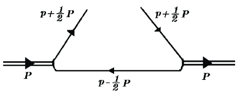
Figure 11: Diagrammatic contributions to the parton distributions of the pion.

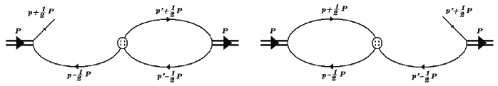
Figure 12: Diagrammatic contributions to the parton distributions of the pion.

The corresponding diagrams are those shown of Figs. 11 and 12.

We can split the parton distribution into two one body and one two body contributions

$$q\left(x\right)=q^{\left(1\right)}\left(x\right)+\tilde{q}^{\left(1\right)}\left(x\right)+q^{\left(2\right)}\left(x\right)\ .$$ (VII.12)

The first contribution, $q^{\left(1\right)}\left(x\right),$ is the one appearing in equation (VII.9) and corresponds to the diagram shown in Fig. 11. The second term is also a one body term,

$$\tilde{q}^{\left(1\right)}\left(x\right)=\int\frac{d^{4}p}{\left(2\pi\right)^{4}}\frac{1}{4}\delta\left(x-\frac{n}{2}\cdot\left(2p+P\right)\right)\mathbb{T}\mathrm{r}\left[in_{\mu}~{}\frac{d\bar{\Gamma}^{M}\left(p,P\right)}{dp_{\mu}}\,i\,S\left(p+\frac{1}{2}P\right)\Gamma^{M}\left(p,P\right)i\,S\left(p-\frac{1}{2}P\right)\right.$$

$$+\left.i\,S\left(p-\frac{1}{2}P\right)\bar{\Gamma}^{M}\left(p,P\right)i\,S\left(p+\frac{1}{2}P\right)in_{\mu}~{}\frac{d\Gamma^{M}\left(p,P\right)}{dp_{\mu}}\right]\ ,$$ (VII.13)

while the third term is a genuine two body term given by,

$$q^{\left(2\right)}\left(x\right)=\int\frac{d^{4}p}{\left(2\pi\right)^{4}}\int\frac{d^{4}p^{\prime}}{\left(2\pi\right)^{4}}\,\left[i\,S\left(p^{\prime}-\frac{1}{2}P\right)\bar{\Gamma}^{M}\left(p^{\prime},P\right)i\,S\left(p^{\prime}+\frac{1}{2}P\right)\right]_{\alpha\gamma}$$

$$\frac{1}{2}n_{\mu}~{}\left\{\left[\delta\left(x-\frac{n}{2}\cdot\left(2p+P\right)\right)\left(\frac{d}{dp_{\mu}^{\prime}}+2\frac{d}{dP_{\mu}}\right)+\delta\left(x-\frac{n}{2}\cdot\left(2p^{\prime}+P\right)\right)\left(\frac{d}{dp_{\mu}}+2\frac{d}{dP_{\mu}}\right)\right]G_{\alpha\beta\gamma\delta}\left(p^{\prime},p,P\right)\right\}$$

$$\left[\,i\,S\left(p+\frac{1}{2}P\right)\Gamma^{M}\left(p,P\right)i\,S\left(p-\frac{1}{2}P\right)\right]_{\beta\delta}\ .$$ (VII.14)

These last two contributions correspond to the diagram of Fig 12 . In $\tilde{q}^{\left(1\right)}\left(x\right)$ the bubble integral has been performed using the BSE, that is the reason for appearing as a one body term.

The whole contribution coming from the diagram of Fig 12 has a non-vanishing contributions to $q\left(x\right),$ nevertheless, when we integrate over $x$ the only non-vanishing contribution that can survive is the one associated to the derivative of the total momentum, which contributes to the form factor. An analysis of this operator in the scenarios here considered is done in NogueraVento05 .

Summarizing, we have three contributions: the standard one, associated with the handbag diagram, and defined in equation (VII.9) and two new contributions defined in Eqs. (VII.13) and (VII.14). These contributions are a consequence of the non locality of the currents involved in our model. From the point of view of QCD they are also handbag diagrams, but in terms of the BS amplitudes they have a different structure.

VIII Conclusion.

We have defined a family of phenomenological chirally invariant non local lagrangians to describe hadron structure. They lead to non trivial momentum dependencies in the quark propagator parametrized by momentum dependent quark mass terms and wave function renormalization constants. We have shown that the formalism is able to emulate any propagator obtained from more fundamental studies. In particular we have studied two scenarios obtained from low energy models of QCD DyakonovPetrov86 , and lattice QCD Bowman02 ; Bowman03 . As a first goal, our lagrangian description allows a careful study of the properties of any observable. In particular we have applied it in detail to the study of the pion electromagnetic form factor with special emphasis to the consequences of the local gauge invariance.

Several authors have previously used non local models, in particular the non local generalization of the Nambu- Jona Lasinio model Birse95 ; Birse98 ; Osipov95 ; GomezDummScoccola04 ; Scoccola01-04 and the instanton liquid model Dorokhov1 , and have studied electromagnetic properties Dorokhov2 ; Dorokhov3 . There are main differences between these approaches and ours. The momentum dependence in our case arises from QCD and appears not only in the mass but also in the wave function renormalization. Moreover, we do not use a separable approximation of the interaction kernel in each particle momentum.

In order to test the consistency of the model, we have studied the basic properties of the theory, i. e. effective current masses and quark condensate. We have constructed, using our models, the two body quark anti-quark bound state equation and solved for the pion obtaining its mass and its Bethe-Salpeter amplitude.

We have implemented the electromagnetic coupling in this theory. The construction of the dressed quark-photon vertex is complicated and the WTI do not solve the problem completely. In particular the transverse propagator has been a subject of much debate. In our lagrangian formalism it is natural to implement local gauge invariance through links between the points where the quark fields act. We find that two new terms appear in the quark-photon vertex which restore local gauge symmetry. We have obtained simple expressions for these two new terms choosing the link between the two points characterizing the non local currents as a straight line. They appear as derivatives of the mass, $m\left(p\right)$, and wave function renormalization, $Z\left(p\right)$, of the quarks. We apply our formalism to the pion form factor and find out that the local gauge restoring terms could amount to as much as 20-30%. Our analysis is applicable to previous work, where the Ball-Chiu prescription for the electromagnetic vertex were used.

We have applied the same ideas to the axial current, implementing local gauge invariance under SU${}_{L}\left(2\right)$ transformations in the lagrangian. We have obtained the full dressed axial vertex. We have discussed several equivalent ways for calculating the pion decay constant. The calculated pion decay constant is in reasonably good agreement with the experimental result. Moreover, we can observe that the two scenarios studied in the paper describe the same physics. It must be emphasized that this two scenarios have a quite different origin.

The basic relations from chiral symmetry, the Goldberger-Treiman and the Gell-Mann-Oakes-Renner relations, have been recovered.

The simplest expression for the axial current, given in equation (V.14), is a good approximation for the calculation of $f_{\pi}$. Nevertheless it does not include the pion pole contribution. Equation (V.15) provides an expression for the longitudinal part of the axial current consistent with PCAC.

Another effect of local gauge invariance is that a new vertex with four quark lines and one photon line appears. The contribution of this vertex to the pion form factor vanishes for our models. This is not a general result, but a consequence of the separable nature and $P-$independence of the interacting terms in our lagrangian. For a general kernel we have seen that this term is necessary in order to guarantee the normalization of the form factor, $F\left(0\right)=1.$

Searching for an observable which is sensitive to this term we have studied the parton distribution. Following the ideas of ref NogueraTheusslVento04 we have obtained the related operator which is path independent and therefore can be used in any other model. The new two body term will give a non vanishing contribution to the parton distribution even within our models NogueraVento05 .

Regarding the numerical values we observe that the two studied scenarios give quite similar results. We only fit $m_{\mathbf{0}}$ in order to reproduce $m_{\pi}$. Their analytic form for the mass, given in equation (II.23) and (II.24), are quite different, but their numerical value in the region $p_{E}^{2}<6\operatorname{GeV}^{2}$ is similar. We regard these expressions as approximations of more realistic expressions for the propagator. In this way, their unwanted analytic properties are not considered. We conclude that both scenarios provide an overall good agreement with the data. The value of the condensate is well reproduced, the value of $m_{0}$ is in agreement with the quark current mass, the value of the pion decay constant is 10% smaller than the experimental value, and both scenarios give similar results. We observe that the fact that $Z\left(p\right)\neq 1$ in the second scenario is not important in these observables. The mean square radius discriminates between these scenarios. In the S1 (S2) we obtain a value which is 10% (20%) smaller than the experimental one. Our analysis shows that this difference is not associated to the different choice of the mass expression but to the fact that in the S2 $Z\left(p\right)\neq 1.$ The electromagnetic radius of the pion will be affected by the coupling of the photon to the meson vectors. This contribution has been estimated to be around the 10-20% MarisTandi00 ; OconnellPearceThomasWilliams97 . The intermediate region, $k^{2}\sim 0.6-0.8\operatorname{GeV}^{2}$, will be also affected by these vector currents through axial components in the pion Bethe-Salpeter amplitude. Therefore we cannot conclude which of the two models is more accurate at present.

In summary we have set the formalism for the description of non local models of hadron structure and have used them to analyze past developments and propose future studies. In particular, it has been already applied for the study of the parton distribution of the pion NogueraVento05 .

Appendix A The quark photon vertex

Let us detail here some intermediate steps related with section IV.

The set of eight basic transverse tensors $T_{i}^{\mu}\left(p_{1},p_{2}\right)$ we use in equation (IV.3) are those defined by Ball and Chiu BallChiu80 with some minor modifications $\left(k=p_{2}-p_{1}\right)$,

$$T_{1}^{\mu}\left(p_{1},p_{2}\right) =p_{1}^{\mu}\left(p_{2}.k\right)-p_{2}^{\mu}\left(p_{1}.k\right)\;,$$

$$T_{2}^{\mu}\left(p_{1},p_{2}\right) =\left[p_{1}^{\mu}\left(p_{2}.k\right)-p_{2}^{\mu}\left(p_{1}.k\right)\right]\frac{\left(\hbox to0.0pt{$/$\hss}p_{1}+\hbox to0.0pt{$/$\hss}p_{2}\right)}{2}\;,$$

$$T_{3}^{\mu}\left(p_{1},p_{2}\right) =k^{2}\gamma^{\mu}-k^{\mu}\hbox to0.0pt{$/$\hss}k\;,$$

$$T_{4}^{\mu}\left(p_{1},p_{2}\right) =-i\left[p_{1}^{\mu}\left(p_{2}.k\right)-p_{2}^{\mu}\left(p_{1}.k\right)\right]p_{1}^{\lambda}p_{2}^{\nu}\sigma_{\lambda\nu}\;,$$

$$T_{5}^{\mu}\left(p_{1},p_{2}\right) =-i\sigma^{\mu\lambda}k_{\lambda}\;,$$ (A.15)

$$T_{6}^{\mu}\left(p_{1},p_{2}\right) =\gamma^{\mu}\left(p_{2}^{2}-p_{1}^{2}\right)-\left(p_{1}+p_{2}\right)^{\mu}\hbox to0.0pt{$/$\hss}k\;,$$

$$T_{7}^{\mu}\left(p_{1},p_{2}\right) =\frac{p_{2}^{2}-p_{1}^{2}}{2}\left[\gamma^{\mu}\left(\hbox to0.0pt{$/$\hss}p_{1}+\hbox to0.0pt{$/$\hss}p_{2}\right)-p_{1}^{\mu}-p_{2}^{\mu}\right]-i\left(p_{1}+p_{2}\right)^{\mu}p_{1}^{\lambda}p_{2}^{\nu}\sigma_{\lambda\nu}\;,$$

$$T_{8}^{\mu}\left(p_{1},p_{2}\right) =i\gamma^{\mu}p_{1}^{\lambda}p_{2}^{\nu}\sigma_{\lambda\nu}+p_{1}^{\mu}\hbox to0.0pt{$/$\hss}p_{2}-p_{2}^{\mu}\hbox to0.0pt{$/$\hss}p_{1}\;.$$

Looking at the four quark photon vertex, we must expand the exponential with the $A_{\mu}\left(z\right)$ field in the currents of Eqs.(IV.4-IV.6). Let us start with the scalar current equation (IV.4)

$$J_{S}\left(x\right) =J_{S}^{\left(0A\right)}\left(x\right)+J_{S}^{\left(1A\right)}\left(x\right)+....=\int d^{4}y\,G_{0}\left(y\right)\bar{\psi}\left(x+\frac{1}{2}y\right)~{}\psi\left(x-\frac{1}{2}y\right)+$$ (A.16a)

$$\int d^{4}y\,G_{0}\left(y\right)\bar{\psi}\left(x+\frac{1}{2}y\right)~{}\left(-iQ\int_{x-\frac{1}{2}y}^{x+\frac{1}{2}y}dz^{\mu}A_{\mu}\left(z\right)\right)~{}\psi\left(x-\frac{1}{2}y\right)+...\ \ \ .$$ (A.16b)

Inserting this expansion in the $J_{S}^{\dagger}\left(x\right)J_{S}\left(x\right)$ term of equation (II.4), the first crossed term, $J_{S}^{\left(0A\right){\dagger}}\left(x\right)J_{S}^{\left(1A\right)}\left(x\right)+J_{S}^{\left(1A\right){\dagger}}\left(x\right)J_{S}^{\left(0A\right)}\left(x\right),$ leads to the 4 quarks-photon vertex. An evaluation of this vertex needs to specify the path from $x-\frac{1}{2}y$ to $x+\frac{1}{2}y$ followed by the evaluation of the integral on $z^{\mu}$ in equation (A.16b). This path can be parameterized as

$$z^{\mu}=x^{\mu}+\frac{\lambda}{2}y^{\mu}+c_{\text{{S}}}^{\mu}\left(\lambda\right)\text{~{}~{}~{}~{}with~{}~{}~{}~{}}\lambda\in\left[-1,1\right]\text{~{}~{}~{}~{}and~{}~{}~{}~{}}c_{\text{{S}}}^{\mu}\left(-1\right)=c_{\text{{S}}}^{\mu}\left(1\right)=0\ \ .$$ (A.17)

The current $J_{S}^{\left(1A\right)}\left(x\right)$ between states of 1 quark of momentum $p_{1},$ and 1 photon-1 quark of momentum $k$ and $p_{3},$ respectively gives

$$\left\langle p_{3}\left|J_{S}^{\left(1A\right)}\left(x\right)\right|p_{1}k\right\rangle =\bar{u}\left(p_{3}\right)\left(-iQ\right)u\left(p_{1}\right)e^{i\left(p_{3}-k-p_{1}\right)x}\epsilon^{\mu}\left(k,\xi\right)\int\frac{d^{4}t}{\left(2\pi\right)^{4}}G_{0}\left(t\right)$$

$$\int d^{4}y\,\left(\int_{-1}^{1}d\lambda\left(\frac{1}{2}y_{\mu}+c_{\text{{S}}\mu}^{\prime}\right)e^{-ikc_{\text{{S}}}}\right)e^{iy\left(\frac{p_{1}+p_{3}-\lambda k}{2}-t\right)}$$

$$=\bar{u}\left(p_{3}\right)\left(-iQ\right)u\left(p_{1}\right)e^{i\left(p_{3}-k-p_{1}\right)x}\epsilon^{\mu}\left(k,\xi\right)$$

$$\int_{-1}^{1}d\lambda\;e^{ikc_{\text{{S}}}}\;\left(-\left(\frac{p_{1}+p_{3}-\lambda k}{2}\right)_{\mu}iG_{0}^{\prime}\left(t\right)+c_{\text{{S}}\mu}^{\prime}G_{0}\left(t\right)\right)_{t=\frac{p_{1}+p_{3}-\lambda k}{2}}\ ,$$ (A.18)

where $Q=e\left(\vec{\tau}.\hat{n}+1/3\right)/2$ is the charge of the quark, $G_{0}^{\prime}\left(t\right)=dG_{0}\left(t\right)/dt^{2}$ and $\epsilon^{\mu}\left(k,\xi\right)$ is the photon polarization. For the sake of simplicity we take $c_{\text{{S}}\mu}=0$ which corresponds to linking the two points of the non local current by a straight line. We can write the matrix element in the following way

$$\left\langle p_{3}\left|J_{S}^{\left(1A\right)}\left(x\right)\right|p_{1}k\right\rangle=-\bar{u}\left(p_{3}\right)~{}Q~{}u\left(p_{1}\right)e^{i\left(p_{3}-k-p_{1}\right)x}\epsilon^{\mu}\left(k,\xi\right)$$

$$\left[\left(p_{1}+p_{3}\right)_{\mu}\mathbb{V}_{0a}\left(\frac{p_{1}+p_{3}}{2},k\right)-k_{\mu}\mathbb{V}_{0b}\left(\frac{p_{1}+p_{3}}{2},k\right)\right]\ ,$$ (A.19)

where

$$\mathbb{V}_{0a}\left(\bar{p},k\right)=\int_{-1}^{1}d\lambda\;\frac{1}{2}G_{0}^{\prime}\left(\bar{p}-\lambda\frac{k}{2}\right)\ ,$$ (A.20a)

$$\mathbb{V}_{0b}\left(\bar{p},k\right)=\int_{-1}^{1}d\lambda\;\frac{\lambda}{2}\;G_{0}^{\prime}\left(\bar{p}-\lambda\frac{k}{2}\right)\ .$$ (A.20b)

Using the current given in equation (A.19) we obtain the vertex associated to the interacting term $$g_{0}\left(J_{S}^{\left(0A\right){\dagger}}\left(x\right)J_{S}^{\left(1A\right)}\left(x\right)+J_{S}^{\left(1A\right){\dagger}}\left(x\right)J_{S}^{\left(0A\right)}\left(x\right)\right)$$ of the Lagrangian,

$$\left[\Gamma_{S,\mu}^{(4q\gamma)}\left(p_{1},p_{3};p_{2},p_{4}\right)\right]_{\alpha\beta,\gamma\delta}=-i2g_{0}G_{0}\left(\frac{p_{2}+p_{4}}{2}\right)\delta_{\beta\delta}Q_{\gamma\alpha}\left[\left(p_{1}+p_{3}\right)_{\mu}\mathbb{V}_{0a}\left(\frac{p_{1}+p_{3}}{2},k\right)\right.$$

$$-\left.k_{\mu}\mathbb{V}_{0b}\left(\frac{p_{1}+p_{3}}{2},k\right)\right]+\left(p_{1}\alpha,p_{3}\gamma\leftrightarrow p_{2}\beta,p_{4}\delta\right)\ ,$$ (A.21)

with $k=p_{3}+p_{4}-p_{1}-p_{2}.$

We apply the same ideas to the pseudoscalar current (IV.5) obtaining the vertex associated to the interacting term $g_{0}\left(J_{5}^{\left(0A\right){\dagger}}\left(x\right)J_{5}^{\left(1A\right)}\left(x\right)+J_{5}^{\left(1A\right){\dagger}}\left(x\right)J_{5}^{\left(0A\right)}\left(x\right)\right)$ of the Lagrangian,

$$\left[\Gamma_{5,\mu}^{(4q\gamma)}\left(p_{1},p_{3};p_{2},p_{4}\right)\right]_{\alpha\beta,\gamma\delta}=-i2g_{0}G_{0}\left(\frac{p_{2}+p_{4}}{2}\right)\left(i\gamma_{5}\vec{\tau}\right)_{\delta\beta}$$

$$\left\{\left(i\gamma_{5}\frac{1}{2}\left\{Q,\vec{\tau}\right\}\right)_{\gamma\alpha}\left[\left(p_{1}+p_{3}\right)_{\mu}\mathbb{V}_{0a}\left(\frac{p_{1}+p_{3}}{2},k\right)-k_{\mu}\mathbb{V}_{0b}\left(\frac{p_{1}+p_{3}}{2},k\right)\right]\right.+$$

$$\left.\left(i\gamma_{5}\frac{1}{2}\left[Q,\vec{\tau}\right]\right)_{\gamma\alpha}\left[\left(p_{1}+p_{3}\right)_{\mu}\mathbb{A}_{0a}\left(\frac{p_{1}+p_{3}}{2},k\right)-k_{\mu}\mathbb{A}_{0b}\left(\frac{p_{1}+p_{3}}{2},k\right)\right]\right\}+\left(p_{1}\alpha,p_{3}\gamma\leftrightarrow p_{2}\beta,p_{4}\delta\right)\ ,$$ (A.22)

with

$$\mathbb{A}_{0a}\left(\bar{p},k\right) =\int_{0}^{1}d\lambda\;\frac{1}{2}G_{0}^{\prime}\left(\bar{p}-\lambda\frac{k}{2}\right)-\int_{-1}^{0}d\lambda\;\frac{1}{2}G_{0}^{\prime}\left(\bar{p}-\lambda\frac{k}{2}\right)\ ,$$ (A.23a)

$$\mathbb{A}_{0b}\left(\bar{p},k\right) =\int_{0}^{1}d\lambda\;\frac{\lambda}{2}\;G_{0}^{\prime}\left(\bar{p}-\lambda\frac{k}{2}\right)-\int_{-1}^{0}d\lambda\;\frac{\lambda}{2}\;G_{0}^{\prime}\left(\bar{p}-\lambda\frac{k}{2}\right)\ .$$ (A.23b)

and $$\mathbb{V}_{0a} \mathbb{V}_{0b}$$ and given in equations (A.20a) and (A.20b).

The momentum current equation (IV.6) produces the interacting term $g_{p}\left(J_{p}^{\left(0A\right){\dagger}}\left(x\right)J_{p}^{\left(1A\right)}\left(x\right)+J_{p}^{\left(1A\right){\dagger}}\left(x\right)J_{p}^{\left(0A\right)}\left(x\right)\right).$ The associated vertex is

$$\left[\Gamma_{p,\mu}^{(4q\gamma)}\left(p_{1},p_{3};p_{2},p_{4}\right)\right]_{\alpha\beta,\gamma\delta}=-i2g_{p}G_{p}\left(\frac{p_{2}+p_{4}}{2}\right)\left(\frac{\hbox to0.0pt{$/$\hss}p_{2}+\hbox to0.0pt{$/$\hss}p_{4}}{2}\right)_{\delta\beta}\left(Q\gamma^{\nu}\right)_{\gamma\alpha}$$

$$\left\{g_{\nu\mu}\frac{1}{2}\left[G_{p}\left(\frac{p_{1}+p_{3}+k}{2}\right)+G_{p}\left(\frac{p_{1}+p_{3}-k}{2}\right)\right]\right.$$

$$+\left.\frac{\left(p_{1}+p_{3}\right)_{\nu}}{2}\left[\left(p_{1}+p_{3}\right)_{\mu}\mathbb{V}_{pa}\left(\frac{p_{1}+p_{3}}{2},k\right)-k_{\mu}\mathbb{V}_{pb}\left(\frac{p_{1}+p_{3}}{2},k\right)\right]\right\}+\left(p_{1}\alpha,p_{3}\gamma\leftrightarrow p_{2}\beta,p_{4}\delta\right)\ ,$$ (A.24)

whith

$$\mathbb{V}_{pa}\left(\bar{p},k\right)=\int_{-1}^{1}d\lambda\;\frac{1}{2}~{}G_{p}^{\prime}\left(\bar{p}-\lambda\frac{k}{2}\right)\ ,$$ (A.25a)

$$\mathbb{V}_{pb}\left(\bar{p},k\right)=\int_{-1}^{1}d\lambda\;\frac{\lambda}{2}\;G_{p}^{\prime}\left(\bar{p}-\lambda\frac{k}{2}\right)\ .$$ (A.25b)

Appendix B The quark $W^{\mu}$ vertex.

Let us decompose the quark field in its left a right parts, $\psi^{L,R}\left(x\right)=\frac{1}{2}\left(1\mp\gamma_{5}\right)\psi\left(x\right).$ Under a local $SU_{L}\left(2\right)$ gauge transformations we have

$$\psi^{L}\left(x\right) \longrightarrow e^{ig_{w}\frac{\vec{\tau}}{2}.\vec{\alpha}\left(x\right)}\psi^{L}\left(x\right)\qquad\psi^{R}\left(x\right)\longrightarrow\psi^{R}\left(x\right)$$ (B.26)

$$\vec{\tau}\vec{W}^{\mu}\left(x\right) =\vec{\tau}\vec{W}^{\mu}\left(x\right)-\partial^{\mu}\vec{\alpha}\left(x\right).\vec{\tau}-g_{w}~{}\left(\vec{\alpha}\left(x\right)\times\vec{W}^{\mu}\left(x\right)\right).\vec{\tau}~{}~{}.$$ (B.27)

Our lagrangian model defined in (II.4) is invariant under infinitesimal global gauge $SU_{L}\left(2\right)$ transformation. Now we are interested in making this lagrangian invariant under local transformations. We proceed in a similar way as in the electromagnetic case. The main difficulty is on the fact that our currents are built with fields in different points, thus the value of $\vec{\alpha}\left(x\right)$ will be different for each point. To avoid this difficulty let us introduce the following product of fields

$$\mathcal{P}\left(e^{-i\frac{g_{w}}{2}\int_{y}^{x}dz^{\mu}~{}\vec{\tau}\vec{W}^{\mu}\left(z\right)}\right)~{}\psi^{L}\left(y\right)$$ (B.28)

which transform covariantly at least for infinitesimal transformations,

$$\left[e^{-i\frac{g_{w}}{2}\int_{y}^{x}dz^{\mu}~{}\vec{\tau}\vec{W}^{\mu}\left(z\right)}~{}\psi^{L}\left(y\right)\right]\longrightarrow e^{i\frac{g_{w}}{2}\vec{\tau}.\vec{\alpha}\left(x\right)}\left[e^{-i\frac{g_{w}}{2}\int_{y}^{x}dz^{\mu}~{}\vec{\tau}\vec{W}^{\mu}\left(z\right)+\mathcal{O}\left(g_{w}^{2}\right)}~{}\psi^{L}\left(y\right)\right]$$ (B.29)

Then, we can define the currents

$$J_{S}\left(x\right) =\int d^{4}y\,G_{0}\left(y\right)\left[\bar{\psi}^{R}\left(x+\frac{1}{2}y\right)~{}\mathcal{P}\left(e^{-i\frac{g_{w}}{2}\int_{x-\frac{1}{2}y}^{x}dz^{\mu}\vec{W}_{\mu}\left(z\right)\vec{\tau}}\right)~{}\psi^{L}\left(x-\frac{1}{2}y\right)\right.$$

$$~{}~{}~{}~{}~{}~{}~{}~{}~{}~{}~{}~{}~{}~{}~{}~{}~{}~{}~{}~{}+\left.\bar{\psi}^{L}\left(x+\frac{1}{2}y\right)~{}\mathcal{P}\left(e^{-i\frac{g_{w}}{2}\int_{x}^{x+\frac{1}{2}y}dz^{\mu}\vec{W}_{\mu}\left(z\right)\vec{\tau}}\right)~{}\psi^{R}\left(x-\frac{1}{2}y\right)\right]\ ,$$ (B.30)

$$\vec{J}_{5}\left(x\right) =\int d^{4}y\,G_{0}\left(y\right)\left[-i~{}\bar{\psi}^{R}\left(x+\frac{1}{2}y\right)~{}\vec{\tau}~{}\mathcal{P}\left(e^{-i\frac{g_{w}}{2}\int_{x-\frac{1}{2}y}^{x}dz^{\mu}\vec{W}_{\mu}\left(z\right)\vec{\tau}}\right)~{}\psi^{L}\left(x-\frac{1}{2}y\right)\right.$$

$$~{}~{}~{}~{}~{}~{}~{}~{}~{}~{}~{}~{}~{}~{}~{}~{}~{}~{}~{}~{}+\left.i~{}\bar{\psi}^{L}\left(x+\frac{1}{2}y\right)~{}\mathcal{P}\left(e^{-i\frac{g_{w}}{2}\int_{x}^{x+\frac{1}{2}y}dz^{\mu}\vec{W}_{\mu}\left(z\right)\vec{\tau}}\right)~{}\vec{\tau}~{}\psi^{R}\left(x-\frac{1}{2}y\right)\right]\ ,$$ (B.31)

$$J_{p}\left(x\right) =\int d^{4}y\,G_{p}\left(y\right)\frac{1}{2}\left[\bar{\psi}^{L}\left(x+\frac{1}{2}y\right)~{}\mathcal{P}\left(e^{-i\frac{g_{w}}{2}\int_{x-\frac{1}{2}y}^{x+\frac{1}{2}y}dz^{\mu}\vec{W}_{\mu}\left(z\right)\vec{\tau}}\right)~{}i\ \hbox to0.0pt{$/$\hss}D\ \psi^{L}\left(x-\frac{1}{2}y\right)\right.$$

$$~{}~{}~{}~{}~{}~{}~{}~{}~{}~{}~{}~{}~{}~{}~{}~{}\ \ \ \ \ \ \ \ -i\bar{\psi}^{L}\left(x+\frac{1}{2}y\right)\overleftarrow{\hbox to0.0pt{$/$\hss}D}~{}\mathcal{P}\left(e^{-i\frac{g_{w}}{2}\int_{x-\frac{1}{2}y}^{x+\frac{1}{2}y}dz^{\mu}\vec{W}_{\mu}\left(z\right)\vec{\tau}}\right)~{}\psi^{L}\left(x-\frac{1}{2}y\right)$$

$$~{}~{}~{}~{}~{}~{}~{}~{}~{}~{}~{}~{}~{}~{}~{}~{}~{}~{}~{}~{}+\left.i\bar{\psi}^{R}\left(x+\frac{1}{2}y\right)\overleftrightarrow{\hbox to0.0pt{$/$\hss}\partial}~{}\psi^{R}\left(x-\frac{1}{2}y\right)\right]\ ,$$ (B.32)

where the covariant derivative is $D^{\mu}\psi\left(x\right)=\left[\partial^{\mu}+ig_{w}\vec{W}^{\mu}\left(z\right)\frac{\vec{\tau}}{2}\right]\psi^{L}\left(x\right).$ With these definitions, the combination $J_{S}^{2}\left(x\right)+\vec{J}_{5}^{\,2}\left(x\right)$ is invariant under local infinitesimal gauge transformations. The momentum current, $J_{P}\left(x\right),$ is self-invariant.

Once we have the invariant lagrangian we proceed for obtaining the 4quarks-$W^{\mu}$ vertex. The procedure is exactly the same as in the previous appendix, expanding the currents in the number of $W$ mesons, and we write directly our results.

The vertex associated to the interacting term $g_{0}\left(J_{S}^{\left(0W\right){\dagger}}\left(x\right)J_{S}^{\left(1W\right)}\left(x\right)+J_{S}^{\left(1W\right){\dagger}}\left(x\right)J_{S}^{\left(0W\right)}\left(x\right)\right)$ of the Lagrangian, in which a boson of type $W^{1}$ is involved, is

$$\left[\Gamma_{S,\mu}^{(4qW)}\left(p_{1},p_{3};p_{2},p_{4}\right)\right]_{\alpha\beta,\gamma\delta}=-i~{}2g_{0}\frac{g_{w}}{2}G_{0}\left(\frac{p_{2}+p_{4}}{2}\right)\delta_{\beta\delta}\left\{\left[\left(p_{1}+p_{3}\right)_{\mu}\mathbb{V}_{0a}\left(\frac{p_{1}+p_{3}}{2},k\right)\right.\right.$$

$$-\left.k_{\mu}\mathbb{V}_{0b}\left(\frac{p_{1}+p_{3}}{2},k\right)\right]\left(\frac{1}{2}\tau^{1}\right)_{\gamma\alpha}+\left[\left(p_{1}+p_{3}\right)_{\mu}\mathbb{A}_{0a}\left(\frac{p_{1}+p_{3}}{2},k\right)\right.$$

$$\left.-\left.k_{\mu}\mathbb{A}_{0b}\left(\frac{p_{1}+p_{3}}{2},k\right)\right]\left(\frac{1}{2}\tau^{1}\gamma_{5}\right)_{\gamma\alpha}\right\}+\left(p_{1}\alpha,p_{3}\gamma\leftrightarrow p_{2}\beta,p_{4}\delta\right)\ .$$ (B.33)

The vertex associated to the interacting term $g_{0}\left(J_{5}^{\left(0W\right){\dagger}}\left(x\right)J_{5}^{\left(1W\right)}\left(x\right)+J_{5}^{\left(1W\right){\dagger}}\left(x\right)J_{5}^{\left(0W\right)}\left(x\right)\right)$ of the Lagrangian is

$$\left[\Gamma_{5,\mu}^{(4qW)}\left(p_{1},p_{3};p_{2},p_{4}\right)\right]_{\alpha\beta,\gamma\delta}=-i~{}2g_{0}\frac{g_{w}}{2}G_{0}\left(\frac{p_{2}+p_{4}}{2}\right)\left(i\gamma_{5}\tau^{j}\right)_{\beta\delta}\left\{i\left[\left(p_{1}+p_{3}\right)_{\mu}\mathbb{V}_{0a}\left(\frac{p_{1}+p_{3}}{2},k\right)\right.\right.$$

$$-\left.k_{\mu}\mathbb{V}_{0b}\left(\frac{p_{1}+p_{3}}{2},k\right)\right]\left(\frac{1}{2}\left\{\tau^{1},\tau^{j}\right\}\frac{1}{2}\gamma_{5}+\frac{1}{2}\left[\tau^{1},\tau^{j}\right]\frac{1}{2}\right)_{\gamma\alpha}+\left[\left(p_{1}+p_{3}\right)_{\mu}\mathbb{A}_{0a}\left(\frac{p_{1}+p_{3}}{2},k\right)\right.$$

$$\left.-\left.k_{\mu}\mathbb{A}_{0b}\left(\frac{p_{1}+p_{3}}{2},k\right)\right]\left(\frac{1}{2}\left\{\tau^{1},\tau^{j}\right\}\frac{1}{2}+\frac{1}{2}\left[\tau^{1},\tau^{j}\right]\frac{1}{2}\gamma_{5}\right)_{\gamma\alpha}\right\}+\left(p_{1}\alpha,p_{3}\gamma\leftrightarrow p_{2}\beta,p_{4}\delta\right)\ .$$ (B.34)

The vertex associated to the interacting term $g_{p}\left(J_{p}^{\left(0W\right){\dagger}}\left(x\right)J_{p}^{\left(1W\right)}\left(x\right)+J_{p}^{\left(1W\right){\dagger}}\left(x\right)J_{p}^{\left(0W\right)}\left(x\right)\right)$ of the Lagrangian is

$$\left[\Gamma_{p,\mu}^{(4qW)}\left(p_{1},p_{3};p_{2},p_{4}\right)\right]_{\alpha\beta,\gamma\delta}=-i2g_{p}g_{w}G_{p}\left(\frac{p_{2}+p_{4}}{2}\right)\left(\frac{\hbox to0.0pt{$/$\hss}p_{2}+\hbox to0.0pt{$/$\hss}p_{4}}{2}\right)_{\delta\beta}\left(\tau^{1}\gamma^{\nu}\frac{1}{2}\left(1-\gamma_{5}\right)\right)_{\gamma\alpha}$$

$$\left\{g_{\nu\mu}\frac{1}{2}\left[G_{p}\left(\frac{p_{1}+p_{3}+k}{2}\right)+G_{p}\left(\frac{p_{1}+p_{3}-k}{2}\right)\right]\right.$$

$$+\left.\frac{\left(p_{1}+p_{3}\right)_{\nu}}{2}\left[\left(p_{1}+p_{3}\right)_{\mu}\mathbb{V}_{pa}\left(\frac{p_{1}+p_{3}}{2},k\right)-k_{\mu}\mathbb{V}_{pb}\left(\frac{p_{1}+p_{3}}{2},k\right)\right]\right\}+\left(p_{1}\alpha,p_{3}\gamma\leftrightarrow p_{2}\beta,p_{4}\delta\right)\ ,$$ (B.35)

In all these expressions, the momentum transferred is defined as $k=p_{3}+p_{4}-p_{1}-p_{2}.$ The functions $\mathbb{V}_{0a}$, $\mathbb{V}_{0b}$, $\mathbb{A}_{0a}$, $\mathbb{A}_{0b}$, $\mathbb{V}_{pa}$ and $\mathbb{V}_{pb}$ are defined in equations (A.20a), (A.20b), (A.23a), (A.23b), (A.25a) and (A.25b).

The $W^{1}$ boson couples to quarks through the dressed vertex $\left(\Gamma^{\mu}\left(p_{1},p_{2}\right)-\Gamma_{5}^{\mu}\left(p_{1},p_{2}\right)\right)\tau^{1}.$ As in the quark photon vertex discussed in section IV, the full quark $W$ vertex is constructed in a two steps process. The first one is shown in fig. 4 and it consists in the renormalization of the bare quark-$W$ vertex by the 4 quarks one $W$ vertex. The change in the vector part of the vertex is given in equation (IV.7). The axial part is

$$\Gamma_{5,0}^{\mu}\left(p_{1},p_{2}\right)=\gamma^{\mu}\gamma_{5}+\alpha_{0}\left[\left(p_{1}+p_{2}\right)^{\mu}\,\mathbb{A}_{0a}\left(\bar{p},k\right)+k^{\mu}\,\mathbb{A}_{0b}\left(\bar{p},k\right)\right]\gamma_{5}+$$

$$2~{}G_{0}\left(\frac{p_{1}+p_{2}}{2}\right)\frac{\left(p_{1}-p_{2}\right)^{\mu}}{\left(p_{1}-p_{2}\right)^{2}}\gamma_{5}\left[\alpha_{0}+g_{0}F_{1}\left(k\right)\right]-$$

$$\alpha_{p}\frac{1}{2}\left[G_{p}\left(p_{1}\right)+G_{p}\left(p_{2}\right)\right]\mathbb{\gamma}^{\mu}\gamma_{5}-$$

$$\alpha_{p}\frac{\hbox to0.0pt{$/$\hss}p_{1}+\hbox to0.0pt{$/$\hss}p_{2}}{2}\gamma_{5}\left[\left(p_{1}+p_{2}\right)^{\mu}\,\mathbb{V}_{pa}\left(\frac{p_{1}+p_{2}}{2},k\right)+k^{\mu}\,\mathbb{V}_{pb}\left(\frac{p_{1}+p_{2}}{2},k\right)\right]$$ (B.36)

with $F_{1}\left(k\right)$ given by equation (V.10). It is interesting to note that the longitudinal part of $\Gamma_{5,0}^{\mu}\left(p_{1},p_{2}\right)$,

$$\left(p_{2}-p_{1}\right)_{\mu}\Gamma_{5,0}^{\mu}\left(p_{1},p_{2}\right)=S^{-1}\left(p_{2}\right)\gamma_{5}+\gamma_{5}S^{-1}\left(p_{1}\right)+\left(2m_{0}-2g_{0}G_{0}\left(\frac{p_{1}+p_{2}}{2}\right)F_{1}\left(k^{2}\right)\right)\gamma_{5}~{},$$ (B.37)

does not satisfy the WTI (V.1).

The second step is represented in Fig. 5. The associated equation for the vector part of the vertex is given in equation (IV.8) and the final form of the solution is given in equation (IV.10). The axial part of the vertex is governed by the equation

$$i\,\Gamma_{5}^{\mu}\left(p_{1},p_{2}\right)\frac{\tau^{1}}{2}=i\,\Gamma_{5,0}^{\mu}\left(p_{1},p_{2}\right)\frac{\tau^{1}}{2}+$$

$$i\,2\,g_{0}\,G_{0}\left(\frac{p_{1}+p_{2}}{2}\right)\,i\gamma_{5}\tau^{j}\,\int\frac{d^{4}p}{\left(2\pi\right)^{4}}G_{0}\left(p\right)\,\left(-\right)\mathbb{T}\text{r}\left[i\,S\left(p-\frac{k}{2}\right)\,i\gamma_{5}\,\tau^{j}\,i\,S\left(p+\frac{k}{2}\right)\,i\,\Gamma_{5}^{\mu}\left(p-\frac{k}{2},p+\frac{k}{2}\right)\frac{\tau^{1}}{2}\right]$$ (B.38)

with $k=p_{2}-p_{1}.$ This equation can be solved obtaining

$$\Gamma_{5}^{\mu}\left(p_{1},p_{2}\right)=\Gamma_{5,0}^{\mu}\left(p_{1},p_{2}\right)+2g_{0}G_{0}\left(\frac{p_{1}+p_{2}}{2}\right)\left[F_{1}\left(k^{2}\right)+2m_{0}\frac{F_{0}\left(k^{2}\right)}{1-2g_{0}~{}\Pi_{PS}\left(k^{2}\right)}\right]\frac{k^{\mu}}{k^{2}}\gamma_{5}$$ (B.39)

This expression can be rewritten in the form given by equation (V.5).

In equation (V.14) we give an approximated expression for the longitudinal part of $\Gamma_{5,0}^{\mu}\left(p_{1},p_{2}\right).$ From equations (V.14) and (B.37) we have

$$\left(p_{1}-p_{2}\right)_{\mu}\left(\Gamma_{5,0}^{\mu}\left(p_{1},p_{2}\right)-\Gamma_{5,0}^{\prime\mu}\left(p_{1},p_{2}\right)\right)=$$

$$\left[\alpha_{0}~{}G_{0}\left(p_{1}\right)+\alpha_{0}~{}G_{0}\left(p_{2}\right)+2g_{0}~{}G_{0}\left(p\right)~{}F_{1}\left(P^{2}\right)\right]\gamma_{5}$$ (B.40)

with $p_{1,2}=p\pm P/2.$ Inserting equation (B.40) in (V.8) we can evaluate the numerical error produced in the calculation of $f_{\pi}$ through the use of $\Gamma_{5,0}^{\prime\mu}\left(p_{1},p_{2}\right).$ Expanding in powers of $P^{2}$ it is straightforward to obtain that $\Delta f_{\pi}=\mathcal{O}\left(m_{\pi}^{2}\right).$

There are alternatives ways for calculating the pion decay constant in which we cannot use the approximated expression (V.14). For instance, we can consider an interacting pair $q\bar{q}$ which a some point couples to a $W$ boson. We can describe the interaction between the $q\bar{q}$ by the scattering amplitude or using the dressed vertex. This two descriptions must be equivalents and in the proximity of the pion pole we have

$$iP^{\mu}f_{\pi}\frac{i}{P^{2}-m_{\pi}^{2}}\Gamma_{\gamma\alpha}^{\pi}\left(p^{\prime},P\right)=$$

$$\left(-\right)\int\frac{d^{4}p}{\left(2\pi\right)^{4}}2iG_{\alpha\beta\gamma\delta}\left(p^{\prime},p,P\right)\left(i\,S\left(p-\frac{1}{2}P\right)\,\Gamma_{5}^{\mu}\left(p+\frac{1}{2}P,p-\frac{1}{2}P\right)\,\frac{\tau^{j}}{2}\,i\,S\left(p+\frac{1}{2}P\right)\right)_{\beta\delta}$$ (B.41)

Where, in our model, the interaction is

$$G_{\alpha\beta\gamma\delta}\left(p^{\prime},p,P\right)=g_{0}\ G_{0}\left(p^{\prime}\right)G_{0}\left(p\right)\left[\delta_{\gamma\alpha}\delta_{\delta\beta}+\left(i\vec{\tau}\gamma_{5}\right)_{\gamma\alpha}\left(i\vec{\tau}\gamma_{5}\right)_{\delta\beta}\right]+g_{p}\ G_{p}\left(p^{\prime}\right)G_{p}\left(p\right)\left(\hbox to0.0pt{$/$\hss}p^{\prime}\right)_{\gamma\alpha}\left(\hbox to0.0pt{$/$\hss}p\right)_{\delta\beta}~{}~{},$$ (B.42)

and the pion amplitude is

$$\Gamma_{\alpha\gamma}^{\pi}\left(p,P\right)=i\,g_{\pi qq}\,G_{0}\left(p\right)\,\left(i\,\gamma_{5}\,\tau^{i}\right)_{\alpha\gamma}$$ (B.43)

In the right hand side of equation (B.41) we must consider only the pion pole contribution. It is easy to reproduced the result obtained in equation (V.9) for $f_{\pi}$, and is also obvious that we cannot use of the expression (V.14), because we lost the pion pole in the right hand side of equation (B.41).

Appendix C Four quarks-photon vertex in the general case and the value of the form factor at $k^{2}=0$.

The standard normalization condition for the Bethe-Salpeter amplitude is

$$2iP^{\mu}=$$

$$\int\frac{d^{4}p}{\left(2\pi\right)^{4}}\mathbb{T}\text{r}\left[\bar{\Gamma}^{M}\left(p,P\right)i\,\frac{\partial S\left(p+\frac{1}{2}P\right)}{\partial P_{\mu}}\,\Gamma^{M}\left(p,P\right)\,i\,S\left(p-\frac{1}{2}P\right)+\bar{\Gamma}^{M}\left(p,P\right)i\,S\left(p+\frac{1}{2}P\right)\,\Gamma^{M}\left(p,P\right)\,i\,\frac{\partial S\left(p-\frac{1}{2}P\right)}{\partial P_{\mu}}\right]$$

$$-2i\int\frac{d^{4}p}{\left(2\pi\right)^{4}}\frac{d^{4}p^{\prime}}{\left(2\pi\right)^{4}}\left[i\,S\left(p-\frac{1}{2}P\right)\bar{\Gamma}^{M}\left(p,P\right)i\,S\left(p+\frac{1}{2}P\right)\right]_{\alpha\gamma}\frac{\partial G_{\alpha\beta\gamma\delta}\left(p,p^{\prime},P\right)}{\partial P_{\mu}}$$

$$\left[i\,S\left(p^{\prime}+\frac{1}{2}P\right)\,\Gamma^{M}\left(p^{\prime},P\right)\,i\,S\left(p^{\prime}-\frac{1}{2}P\right)\right]_{\beta\delta}\ \ ,$$ (C.44)

where

$$\,\bar{\Gamma}^{M}\left(p,P\right)=\gamma_{0}\left[\Gamma^{M}\left(p,P\right)\right]^{{\dagger}}\gamma_{0}\ .$$ (C.45)

This normalization condition is equivalent to equation(III.6).

A minimal test of consistency of our calculation is that the form factor at $k^{2}=0$ must be 1 for an amplitude normalized with equation (C.44). Usually the form factor is calculated in the impulse approximation, which includes only the triangle diagram shown in Fig. 7. The use of the Ward identity (VII.1) in order to define the electromagnetic vertex in this diagram provides a contribution which coincides with the first integral on the right hand side of equation (C.44). From that we can conclude that the use of the BSE for the pion with a $P$-independent Bethe-Salpeter kernel together with the triangle diagram provides a consistent approximation scheme Roberts96 . For a $P$-dependent kernel this consistency is lost even at $k^{2}=0$ due to the presence of the second integral on the right hand side of equation (C.44).

Let us proof that $F\left(0\right)=1$ from equation (VII.6). We need to expand equation (VII.6) in powers of the photon field. We retain the second term, which is linear in the photon field. We can evaluate it in the limit $k^{2}\rightarrow 0$ without defining a specific path for the integrals present in equation(VII.6), obtaining

$$\left[Q_{1}\int_{X}^{\frac{x^{\prime}-X^{\prime}}{2}+X}dz^{\mu}A_{\mu}\left(z\right)+Q_{2}\int_{-\frac{x^{\prime}+X^{\prime}}{2}+X}^{X}dz^{\mu}A_{\mu}\left(z\right)+Q_{2}\int_{X}^{\frac{x+X^{\prime}}{2}+X}dz^{\mu}A_{\mu}\left(z\right)+Q_{1}\int_{-\frac{x-X^{\prime}}{2}+X}^{X}dz^{\mu}A_{\mu}\left(z\right)\right]$$

$$\underset{k^{2}\rightarrow 0}{\longrightarrow}\epsilon_{\mu}\left(k,\xi\right)\left[-\left(Q_{1}-Q_{2}\right)X^{\prime\mu}+\frac{Q_{1}+Q_{2}}{2}\left(x^{\mu}+x^{\prime\mu}\right)\right]\ .$$ (C.46)

From this last result it is easy to see that the quantity to add to each vertex of the type of Fig. 3 in the limit of $k^{2}\rightarrow 0$, is given by Eqs. (VII.7) and (VII.8).

The electromagnetic form factor in the limit $k^{2}\rightarrow 0,$ including the contributions from Figs.7 and 8, is

$$i\,e\,2\,\bar{P}^{\mu}F\left(0\right)$$

$$=-iQ_{2}\int\frac{d^{4}p}{\left(2\pi\right)^{4}}\,\mathbb{T}\text{r}\left[\Gamma^{M}\left(p,P\right)i\,S\left(p-\frac{1}{2}P\right)\right.\left.\,\,\bar{\Gamma}^{M}\left(p,P\right)\,i\,S\left(p+\frac{1}{2}P\right)\,\,\Gamma^{\mu}\left(p+\frac{1}{2}P,p+\frac{1}{2}P\right)\,i\,S\left(p+\frac{1}{2}P\right)\right]$$

$$-\,i\,Q_{1}\int\frac{d^{4}p}{\left(2\pi\right)^{4}}\,\mathbb{T}\text{r}\left[\Gamma^{M}\left(p,P\right)\,i\,S\left(p-\frac{1}{2}P\right)\,\Gamma^{\mu}\left(p-\frac{1}{2}P,p-\frac{1}{2}P\right)\right.\left.i\,S\left(p-\frac{1}{2}P\right)\,\bar{\Gamma}^{M}\left(p,P\right)\,i\,S\left(p+\frac{1}{2}P\right)\right]$$

$$-\int\frac{d^{4}p}{\left(2\pi\right)^{4}}\int\frac{d^{4}p^{\prime}}{\left(2\pi\right)^{4}}\,\left[i\,S\left(p^{\prime}-\frac{1}{2}P\right)\bar{\Gamma}^{M}\left(p^{\prime},P\right)i\,S\left(p^{\prime}+\frac{1}{2}P\right)\right]_{\alpha\gamma}$$

$$\left\{-iQ_{1}\left[\Gamma_{1,\mu}^{(4q\gamma)}\left(p^{\prime}-\frac{1}{2}P,p^{\prime}+\frac{1}{2}P;p+\frac{1}{2}P,p-\frac{1}{2}P\right)\right]_{\alpha\beta,\gamma\delta}\right.$$

$$\left.-iQ_{2}\left[\Gamma_{2,\mu}^{(4q\gamma)}\left(p^{\prime}-\frac{1}{2}P,p^{\prime}+\frac{1}{2}P;p+\frac{1}{2}P,p-\frac{1}{2}P\right)\right]_{\alpha\beta,\gamma\delta}\right\}\left[\,i\,S\left(p+\frac{1}{2}P\right)\Gamma^{M}\left(p,P\right)i\,S\left(p-\frac{1}{2}P\right)\right]_{\beta\delta}\ .$$ (C.47)

In order to simplify the first two lines of this equation (the one body part) we make use of the WTI, equation (VII.1). For the two body part of the equation we use

$$\left[-iQ_{1}\Gamma_{1,\mu}^{(4q\gamma)}\left(p^{\prime}-\frac{1}{2}P,p^{\prime}+\frac{1}{2}P;p+\frac{1}{2}P,p-\frac{1}{2}P\right)\right]_{\alpha\beta,\gamma\delta} =-iQ_{1}\left(\frac{d}{dp^{\prime\mu}}+\frac{d}{dp^{\mu}}-2\frac{d}{dP^{\mu}}\right)G_{\alpha\beta\gamma\delta}\left(p^{\prime},p,P\right)\ ,$$ (C.48)

$$\left[-iQ_{2}\Gamma_{2,\mu}^{(4q\gamma)}\left(p^{\prime}-\frac{1}{2}P,p^{\prime}+\frac{1}{2}P;p+\frac{1}{2}P,p-\frac{1}{2}P\right)\right]_{\alpha\beta,\gamma\delta} =-iQ_{2}\left(\frac{d}{dp^{\prime\mu}}+\frac{d}{dp^{\mu}}+2\frac{d}{dP^{\mu}}\right)G_{\alpha\beta\gamma\delta}\left(p^{\prime},p,P\right)\ .$$ (C.49)

Equation (VII.5) allows to do some of these integrals. Charge conjugation symmetry leads to

$$\int\frac{d^{4}p}{\left(2\pi\right)^{4}}\mathbb{T}\text{r}\left[\frac{d~{}\bar{\Gamma}^{M}\left(p,P\right)}{dp^{\mu}}\,i\,S\left(p+\frac{1}{2}P\right)\Gamma^{M}\left(p,P\right)i\,S\left(p-\frac{1}{2}P\right)\right]$$

$$=\int\frac{d^{4}p}{\left(2\pi\right)^{4}}\mathbb{T}\text{r}\left[i\,S\left(p-\frac{1}{2}P\right)\bar{\Gamma}^{M}\left(p,P\right)i\,S\left(p+\frac{1}{2}P\right)\frac{d~{}\Gamma^{M}\left(p,P\right)}{dp^{\mu}}\right]=0\ \ .$$ (C.50)

With these inputs, the normalization condition of the Bethe-Salpeter amplitude, equation (C.44), implies the natural normalization for the form factor, $F\left(0\right)=1.$ We observe that only the contribution associated with the derivative of the total momentum in Eqs.(C.48) and (C.49) gives a non vanishing result.

Our results show that consistency between the Bethe-Salpeter normalization condition equation (C.44) and the value of the meson form factor at $k^{2}=0$ is also attainable for a $P$-dependent kernel, if we add the contributions coming from the diagrams of Figs. 7 and 8. This result is consistent with field theory. We have simply added all the diagrams with a one photon coupling, no matter where the photon couples in our system, and in this way we have obtained the gauge invariant contribution to the form factor. Fig. 8 confirms that the use of the Ward-Takahashi identities for the components of a system is not sufficient to assure that the gauge symmetry is satisfied for the composite system.

References

(1)H. Fritzsch, M. Gell-Mann and H. Leutwyler, Phys. Lett.
B47, 365 (1973).
(2)D.J. Gross and F. Wilczek, Phys. Rev. Lett.30, 1343
(1973), Phys. Rev. D8 3633 (1973); H. D. Politzer, Phys. Rev.
Lett.30 1346 (1973), Phys. Rep. 14, 129 (1974).
(3)K.G. Wilson, Phys.Rev. D10, 2445 (1974).
(4)J.B. Kogut and L. Susskind, Phys. Rev D11, 395 (1975).
(5)N. Brambilla, Antonio Pineda, Joan Soto and A. Vairo,
Nucl.Phys. B566, 275 (2000).
(7)J. Gasser and H. Leutwyler, Ann. Phys. (N.Y.) 158, 142 (1983).
(8)N. Isgur and M. B. Wise, Phys. Lett. B232, 113 (1989),
Phys. Lett. B237, 527 (1990).
(9)A. De Rujula, Howard Georgi and S.L. Glashow, Phys. Rev.
D12, 147 (1975); N. Isgur and G. Karl, Phys. Rev. D 18, 4187 (1978);
Phys. Rev. D 19, 2653 (1979).
(10)A. Manohar and H. Georgi, Nucl. Phys. B234, 189 (1984).
(11)A. Chodos, R.L. Jaffe, K. Johnson, Charles B. Thorn, V.F.
Weisskopf Phys. Rev.D9, 3471 (1974); T. DeGrand, R.L. Jaffe, K.
Johnson and J.E. Kiskis, Phys. Rev. D12, 2060 (1975).
(12)G.E. Brown, M. Rho and V. Vento, Phys. Lett. B84, 383
(1979); V. Vento, M. Rho, E. M. Nyman, J.H. Jun and G.E. Brown Nucl.Phys.
A345, 413 (1980).
(13)Y. Nambu and G. Jona-Lasinio, Phys. Rev. 124, 246 (1961).
(50)H. B. O’Connell, B. C. Pearce, A. W.
Thomas and A. G. Williams Prog. Nucl. Part. Phys. 39, 201 (1997).
(51)S. Noguera, L. Theußl and V. Vento
Eur.Phys.J. A20, 483 (2004).
(52)A. Scarpettini, D. Gomez Dumm and N. N.
Scoccola, Phys. Rev.D69, 114018 (2004).
(53)I. General, D. Gomez Dumm and N. N. Scoccola,
Phys.Lett. B506, 267 (2001); D. Gomez Dumm and N. N. Scoccola, Phys.
Rev. D65, 074021 (2002); R.S. Duhau, A.G. Grunfeld, N. N. Scoccola
Phys.Rev. D70, 074026 (2004).
(54)I.V. Anikin, A.E. Dorokhov, L. Tomio, Phys.Part.Nucl.
31, 509 (2000).