We reconsider little-Higgs corrections to precision data. In five models with global symmetries SU(5), SU(6), SO(9) corrections are (although not explicitly) of ‘universal’ type. We get simple expressions for the $\hat{S},\hat{T},W,Y$ parameters, which summarize all effects. In all models $W,Y\geq 0$ and in almost all models $\hat{S}>(W+Y)/2$. Results differ from previous analyses, which are sometimes incomplete, sometimes incorrect, and because we add LEP2 $e\bar{e}\to f\bar{f}$ cross sections to the data set. Depending on the model the constraint on $f$ ranges between $2$ and $20\,{\rm TeV}$.
We next study the ‘simplest’ little-Higgs model (and propose a new related model) which is not ‘universal’ and affects precision data due to the presence of an extra $Z^{\prime}$ vector. By restricting the data-set to the most accurate leptonic data we show how corrections to precision data generated by a generic $Z^{\prime}$ can be encoded in four effective $\hat{S},\hat{T},W,Y$ parameters, giving their expressions.

1 Introduction

While supersymmetric extensions of the Standard Model (SM) technically solve the hierarchy problem, the ever-rising lower bounds on sparticle masses recently stimulated searches for alternative methods of electroweak breaking.

Models where the Higgs (and possibly other SM particles) become extended objects seem generically disfavored by precision data [1], which do not show hints for the expected form factors. Using the QFT language, one expects the presence of extra dimension 6 operators added to the SM Lagrangian. Even if new physics is confined to the Higgs sector, precision data are affected by operators like $|H^{\dagger}D_{\mu}H|^{2}$. Physically, this happens because experiments tested the $W,Z$ bosons, which contain Higgs degrees of freedom in their longitudinal components. Models of this type include technicolor [2], where the Higgs becomes a bound state, and extra-dimensional models that allow TeV-scale quantum gravity [3], where the Higgs supposedly becomes some stringy-like object.

Attempts of improving the situation employ the fact that the Higgs mass can be partially protected from quadratically divergent one loop corrections assuming that the Higgs is a pseudo-Goldstone boson of some global symmetry spontaneously broken at a scale $f$. In order to address the hierarchy problem in this way $f$ must be around the Fermi scale: this has been achieved only recently and only partially by little-Higgs models [4, 5, 6, 7, 8, 9, 10, 11, 12, 13, 14]. The difficulty is that the Higgs does not look like a pseudo-Goldstone boson (the Higgs has sizable interactions with itself and with the top quark), so that one has to invent appropriate ‘epycicles’.

Little Higgs models are mostly characterized by the choice of gauge and global groups. The main free parameters are the gauge coupling(s) of the full gauge group, and the scale $f$ at which the full group is spontaneously broken to the SM group. No specific model seems better than the other ones. Tree level exchange of new heavy vector bosons gives rise to corrections to precision observables. Such corrections also depend on how fermions are introduced. We here stick to the simplest choice made in the original literature, although introducing more ‘epycicles’ gives interesting alternatives [13].

We improve on previous computations and analyses [17, 18, 19, 20, 21, 22, 23] in the following ways. Most little-Higgs models are ‘universal’: all effects can be encoded in four parameters, $\hat{S},\hat{T},W,Y$. As discussed in section 3 this makes results and computations much simpler than in previous analyses that tried to compute corrections to all observables. We include LEP2 data on $e\bar{e}\to f\bar{f}$ cross sections [27, 28], that provide significant constraints on $W,Y$ [25]. In section 2 we critically discuss the robustness of experimental inputs.

In section 4 we consider two ‘littlest’ Higgs models [6, 12], with global symmetry SU(5) and different gauge groups. In section 5 we consider one model with global symmetry SO(9) [11]. In section 6 we consider two little-Higgs models, with global symmetry SU(6) [8, 20] and different gauge groups. All these models are ‘universal’.

In section 8 we consider the ‘simplest’ little-Higgs model [14]. In section 9 we propose and analyze a related little-Higgs model. Both models are not universal and affect precision data plus LEP2 only due to the presence of a heavy $Z^{\prime}$ boson. In the previous section 7 we show how, by considering only the most precise precision data, the effects of generic $Z^{\prime}$ models can be condensed in a set of effective $\hat{S},\hat{T},W,Y$ parameters and compute them.

Section 10 contains our conclusions.

$$\begin{array}[]{rclrlcc}\lx@intercol\hfil\hbox{Adimensional form factors}\hfil\lx@intercol&\lx@intercol\hfil\hbox{operators}\hfil\lx@intercol\\ \hline\cr(g^{\prime}/g){\color[rgb]{0,0,0.4}\widehat{S}}&=&\Pi^{\prime}_{W_{3}B}(0)&{\cal O}_{WB}~{}=&(H^{\dagger}\tau^{a}H)W^{a}_{\mu\nu}B_{\mu\nu}\!\!\!\\[2.84526pt] M_{W}^{2}{\color[rgb]{0,0,0.4}\widehat{T}}&=&\Pi_{W_{3}W_{3}}(0)-\Pi_{W^{+}W^{-}}(0)\!\!\!&{\cal O}_{H}~{}=&|H^{\dagger}D_{\mu}H|^{2}\\[2.84526pt] 2M_{W}^{-2}{\color[rgb]{0,0,0.4}Y}&=&\Pi^{\prime\prime}_{BB}(0)&{\cal O}_{BB}~{}=&(\partial_{\rho}B_{\mu\nu})^{2}/2\\[2.84526pt] 2M_{W}^{-2}{\color[rgb]{0,0,0.4}W}&=&\Pi^{\prime\prime}_{W_{3}W_{3}}(0)&{\cal O}_{WW}~{}=&(D_{\rho}W^{a}_{\mu\nu})^{2}/2\\[2.84526pt] \end{array}$$

Table 1: The first column defines the adimensional form factors. The second column defines the SU(2)_L-invariant universal dimension-6 operators, which contribute to the form-factors on the same row. We use canonically normalized fields and inverse propagators $\Pi$.

2 Experimental data

Our data-set includes all traditional precision electroweak data. Some measurements achieved better than per-mille accuracy. Most data have per-cent accuracy: LEP2 $e\bar{e}\to f\bar{f}$ cross sections, atomic parity violation, Møller scattering, neutrino/nucleon scattering, etc. Despite the larger uncertainty LEP2 plays an important rôle: being the only precision data measured above the $Z$-peak, LEP2 data are particularly sensitive to high-energy new physics.

Before performing a global fit, we discuss its ‘robustness’ i.e. how necessary arbitrary choices affect the final results. Since the data-set contains several observables, on statistical basis one expects a few ‘anomalous’ results. Indeed the data contain three $\sim 3\sigma$ anomalies. Only the first one involves one measurement which has a significant impact in the global fit.

• There is a $3\sigma$ discrepancy between LEP and SLD measurements of the weak angle in leptonic couplings of the $Z$. We do not see how it might be due to new physics. Assuming that the discrepancy is due to a statistical fluctuation, we include both pieces of data in our global fit.

• NuTeV claims that the low-energy couplings of neutrinos to left-handed quarks is $3\sigma$ away from the SM central value. Hadronic uncertainties have not been fully taken into account in the NuTeV results and certain SM effects, such as a $s/\bar{s}$ momentum asymmetry [29], can explain the NuTeV anomaly. Therefore the fit on which our results are based includes all data except NuTeV (second row of table 2).

• The forward/backward asymmetry in $e\bar{e}\to Z\to b\bar{b}$, $A_{FB}^{b}$, is about $3\sigma$ different from its SM prediction. It could be produced by new physics, provided that new physics affects almost only $A_{FB}^{b}$. In fact $A_{FB}^{b}$ has an uncertainty much larger than other observables, where no anomaly is present. Furthermore, the total $Z\to b\bar{b}$ rate is in agreement with the SM.

We have no reason of dropping $A_{FB}^{b}$. Just to verify the stability of our results, in the third row of table 2 we study what happens if both NuTeV and $A_{FB}^{b}$ are dropped. As both pieces of data mildly favor a heavy Higgs, omitting them the best-fit value of the Higgs mass decreases below the direct limit $m_{h}>115\,{\rm GeV}$, unless physics beyond the SM is present. This argument was used in [30] to claim that new physics is needed. However the discrepancy has never been significant, and with the most recent data (in particular for the top mass), the best-fit value of the Higgs mass is only $1\sigma$ too low.

In conclusion, constraints on new physics seem ‘robust’. On the contrary, possible hints for new physics depend on arbitrary choices needed to perform an analysis, like omitting NuTeV and/or $A_{FB}^{b}$ and/or adding LEP2. Since none of these hints is statistically significant we prefer to ignore them.

$$\begin{array}[]{r|cccc|c}\hbox{Type of fit}&1000\,\hat{S}&1000\,\hat{T}&1000\,W&1000\,Y&\chi^{2}_{\rm SM}-\chi^{2}_{\rm min}\\ \hline\cr\hbox{All data}&-0.3&-0.6&-0.7&0.4&1.1^{2}\cr\hbox{Excluding NuTeV (our default fit)}&0&0.2&-0.2&0&0.5^{2}\cr\hbox{Excluding NuTeV and $A_{FB}^{b}$}&-0.9&-0.3&-0.4&0.2&1.2^{2}\cr\end{array}$$

Table 2: Best-fit values for $m_{h}=115\,{\rm GeV}$. The typical uncertainty on $\hat{S},\hat{T},W,Y$ is $\pm 0.5$ with correlations among them. The last column shows that in no case the best fit is significantly better than the SM fit.

3 Computing universal effects

We compute the leading effects, suppressed by one power of $v^{2}/f^{2}$. The analysis is simplified by recognizing that, despite appearances, most little-Higgs models give corrections of ‘universal’ type, that can be fully encoded in the four parameters $\hat{S},\hat{T},W,Y$ defined in [25]. Furthermore, computations are performed with a simplified technique. We repeat here the general presentation of [25] specializing it to the specific case of little-Higgs models.

There are two sets of vector bosons: charged and neutral. Each set involves a few vector bosons $W_{i}$, but all their interactions with the SM fermions can be written as $JW_{1}$, where $W_{1}$ is one linear combination of the $W_{i}$ and $J$ is the standard SM fermionic current. This is why corrections are of ‘universal’ type. The SM contains a few currents $J_{\pm},J_{3},J_{Y}$: to get the essential point we consider a single current and only two vectors $W_{1,2}$.

The mass matrix $m$ of vector bosons $W_{i}$ receives two contributions: one related to the scale $f$ of breaking of the full group, and the usual one related to the scale $v$ of EW symmetry breaking. The model is built such that the SM vector bosons have ${\cal O}(v)$ masses, while all other ones receive ${\cal O}(f)$ masses. The relevant Lagrangian has the schematic form

$$\mathscr{L}\simeq W_{i}\frac{\Pi_{ij}^{\rm full}}{2}W_{j}+gJW_{1},\qquad\Pi_{ij}^{\rm full}=p^{2}\delta_{ij}-m_{ij}^{2}.$$ (1)

The standard computation proceeds by integrating out the heavy mass eigenstates, which are some linear combination of the $W_{i}$: $W_{\rm out}=W_{2}\cos\theta+W_{1}\sin\theta$. In this way one obtains the effective Lagrangian for the light mass eigenstate $W_{\rm in}=W_{1}\cos\theta-W_{2}\sin\theta$. The angle $\theta$ is usually determined such that $W_{\rm out}$ is the heavy mass eigenstate. With more than two vector bosons $\theta$ is replaced by an appropriate unitary matrix.

Let us instead proceed by keeping $\theta$ arbitrary. Keeping terms up to dimension 6, integrating out $W_{\rm out}$ gives rise to an effective Lagrangian of the form

$$\mathscr{L}_{\rm eff}\simeq W_{\rm in}[A(\theta)+B(\theta)p^{2}+C(\theta)p^{4}]W_{\rm in}+W_{\rm in}[D(\theta)+E(\theta)p^{2}]J+F(\theta)J^{2}$$ (2)

i.e. universal corrections $A,B,C$, plus corrections to gauge couplings $D,E$, plus four fermion operators $F$. At this point one can compute any observable.

Alternatively one can recognize that computing all observables is not necessary, because the apparently ‘non-universal’ terms $E$ and $F$ only involve the SM current $J$, and can therefore be eliminated by using the equation of motion of $W_{\rm in}$: $J=-2W_{\rm in}[A+Bp^{2}+Cp^{4}]/[D+Ep^{2}]$. The result is an explicitly ‘universal’ effective Lagrangian of the form with primed coefficients:

$$\mathscr{L}_{\rm eff}\simeq W_{\rm in}[A^{\prime}(\theta)+B^{\prime}(\theta)p^{2}+C^{\prime}(\theta)p^{4}]W_{\rm in}+W_{\rm in}D^{\prime}(\theta)J$$ (3)

With appropriate rescalings of $W_{\rm in}$ and of $g$ it can be rewritten in canonical form

$$\mathscr{L}_{\rm eff}\simeq W_{\rm in}[A^{\prime\prime}(\theta)+p^{2}+C^{\prime\prime}(\theta)p^{4}]W_{\rm in}+W_{\rm in}gJ.$$ (4)

Provided that all above steps have been performed correctly one should find that $A^{\prime\prime}$ and $C^{\prime\prime}$ do not depend on the arbitrary angle $\theta$. Indeed $A^{\prime\prime}$ and $C^{\prime\prime}$ have a direct physical meaning, so that their values cannot depend on how one chooses to compute them. We do not report the explicit verification of this property because the needed computations are more cumbersome than illuminating.

This property suggests a simpler way of computing $A^{\prime\prime}$ and $C^{\prime\prime}$. Rather than finding and integrating out the heavy mass eigenstates (which corresponds to one possible choice of $\theta$), one can more conveniently choose $\theta=0$ and integrate out the vector bosons that do not couple to the SM fermions. In this way there is no need of diagonalizing the mass matrix, and the apparently ‘non-universal’ terms $E$ and $F$ are not generated. Therefore all what one has to do is

1. Given the model, write down the kinetic matrix $\Pi^{\rm full}_{ij}$ of eq. (1).

2. Integrate out all the combinations of extra fields not coupled to SM fermions, obtaining the effective kinetic term $\Pi$ for $W_{1}=W^{+}$ (in the charged sector) or for $W_{1}=\{B,W^{3}\}$ (in the neutral sector). It is given by $\Pi=(\Pi_{\rm full}^{-1}|_{\rm SM})^{-1}$, i.e. one has to restrict the inverse of the full $\Pi$ matrix to the fields coupled to the SM currents, and invert it again, obtaining a $2\times 2$ matrix in the neutral sector and a $1\times 1$ matrix in the charged sector.

3. Expand around $p^{2}\simeq 0$ and extract $\hat{S},\hat{T},W,Y$.

To be concrete, let us apply this procedure to a model that contains one extra heavy vector boson with mass $M$, no mixing to the SM vectors, and that couples to fermions in the same way as the SM hypercharge. The result in the $\{B_{\mu},W^{3}_{\mu}\}$ basis is

$$\Pi^{-1}=\begin{pmatrix}p^{2}-M_{W}^{2}t^{2}&M_{W}^{2}t\cr M_{W}^{2}t&p^{2}-M_{W}^{2}\end{pmatrix}^{-1}+\begin{pmatrix}(p^{2}-M^{2})^{-1}&0\cr 0&0\end{pmatrix}.$$ (5)

This should be intuitively obvious: the first term is the SM contribution; the effect of a vector boson that couples like the SM hypercharge $B_{\mu}$ is taken into account by adding an extra term to the propagator of $B_{\mu}$. From eq. (5) one extracts

$$\hat{S}=Y=\frac{c_{\rm W}^{2}}{s_{\rm W}^{2}}\hat{T}=\frac{M_{W}^{2}}{M^{2}},\qquad W=0$$

which, inserted into [25]

$$\delta\varepsilon_{1}\simeq\widehat{T}-W-Y\frac{s_{\rm W}^{2}}{c_{\rm W}^{2}}\,,\qquad\delta\varepsilon_{2}\simeq-W\,,\qquad\delta\varepsilon_{3}\simeq\widehat{S}-W-Y$$ (6)

gives $\delta\varepsilon_{1,2,3}=0$. Indeed an unmixed hypercharge-like vector affects LEP2 and low-energy observables but does not affect the traditional precision observables $\varepsilon_{1,2,3}$.

Little Higgs models contain various extra vector bosons of this sort, that give tree-level corrections to precision observables. We will study these effects. Two kinds of extra effects might be relevant. First, little-Higgs models employ a heavy top quark to cancel the quadratic divergence associated to the top Yukawa coupling. This heavy new fermion can give one loop corrections to precision observables mainly through $\hat{T}$. Second, some little-Higgs models also contain Higgs ${\rm SU}(2)_{L}$ triplets with vacuum expectation values, which can give arbitrary negative corrections to $\hat{T}$. In these models we present the constraint on $f$, computed under two different assumptions: a) the extra corrections to $\hat{T}$ are negligible; b) the extra corrections to $\hat{T}$ have the value that makes the constraint on $f$ as mild as possible. This kind of analysis may well be considered as exhaustive.

The $99\%$ C.L. constraints on $f$ are computed at fixed values of the other parameters: by making the usual Gaussian approximation we impose $\chi^{2}(f)=\chi^{2}_{\rm SM}+6.6$, which is the value appropriate for 1 degree of freedom. As in [25] we include all precision data expect NuTeV.

      

      

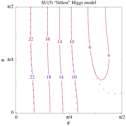
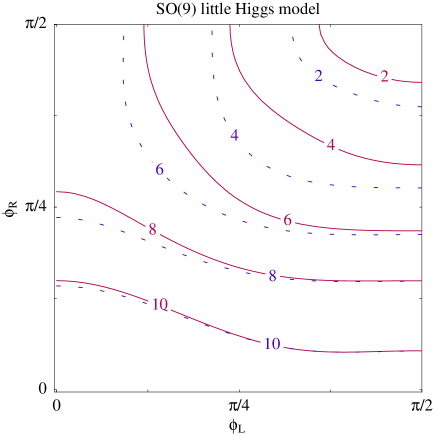
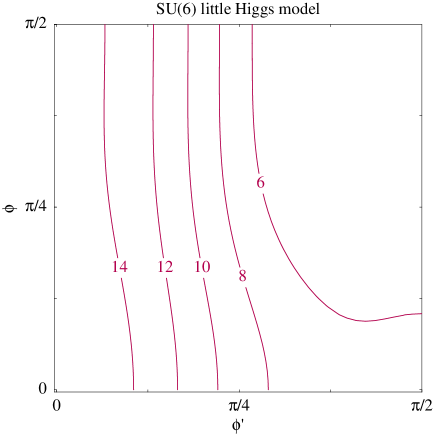
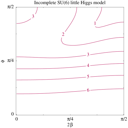
Figure 1: Bound from precision data on the scale $f$ in TeV of little-Higgs models. The constraint is computed at $99\%$ C.L. for 1 dof, i.e. $\chi^{2}=\chi^{2}_{\rm SM}+6.6$. As described in the text in each model the angles $\phi$ parameterize the gauge couplings of the extra gauge groups, which become strongly coupled at $\phi\to 0$ and/or $\phi\to\pi/2$. The dotted iso-lines show that the constraint on $f$ gets slightly relaxed in presence of arbitrary extra corrections to $\hat{T}$. We assumed a light higgs, $m_{h}\sim 115\,{\rm GeV}$.

4 The SU(5)/SO(5) ‘littlest’ Higgs models

This model has a SU(5) global symmetry broken down to SO(5) at the scale $f$. Only the ${\rm SU}(2)_{1}\otimes{\rm SU}(2)_{2}\otimes{\rm U}(1)_{1}\otimes{\rm U}(1)_{2}$ subgroup of SU(5) is gauged, with gauge couplings $g_{1}$, $g_{2}$, $g^{\prime}_{1}$, $g^{\prime}_{2}$ respectively. The SM gauge couplings $g$ and $g^{\prime}$ are obtained as $1/g^{2}=1/g_{1}^{2}+1/g_{2}^{2}$ and $1/g^{\prime 2}=1/g^{\prime 2}_{1}+1/g^{\prime 2}_{2}$. $f$ is normalized such that the heavy vector bosons have masses

$$M_{W^{\prime}}^{2}=\left(g_{1}^{2}+g_{2}^{2}\right)\frac{f^{2}}{4},\hskip 28.45274ptM_{B^{\prime}}^{2}=\left(g^{\prime 2}_{1}+g^{\prime 2}_{2}\right)\frac{f^{2}}{20}.$$ (7)

Matter fermions are charged only under ${\rm SU}(2)_{1}\otimes{\rm U}(1)_{1}$. See [6, 17] for further details. The model has three free parameters, which can be chosen to be $f$ and two angles $\phi$ and $\phi^{\prime}$ defined by

$$\sin\phi=g/g_{1}\hskip 19.91684pt\cos\phi=g/g_{2}\hskip 19.91684pt\sin\phi^{\prime}=g^{\prime}/g^{\prime}_{1}\hskip 19.91684pt\cos\phi^{\prime}=g^{\prime}/g^{\prime}_{2}.$$ (8)

We integrate out the vectors of ${\rm SU}(2)_{2}\otimes{\rm U}(1)_{2}$ under which matter fermions are neutral: therefore neither 4-fermion operators nor corrections to the SM gauge couplings are generated. Only the propagators of the vector bosons coupled to fermions get modified, giving rise to

$$\begin{array}[]{ll}\displaystyle\hat{S}=\frac{2M_{W}^{2}}{g^{2}f^{2}}\bigg{[}\cos^{2}\phi+5\frac{c_{\rm W}^{2}}{s_{\rm W}^{2}}\;\cos^{2}\phi^{\prime}\bigg{]},&\displaystyle W=\frac{4M_{W}^{2}}{g^{2}f^{2}}\cos^{4}\phi,\\ \displaystyle\hat{T}=\frac{5M_{W}^{2}}{g^{2}f^{2}}\ ,&Y=\displaystyle\frac{20M_{W}^{2}}{g^{\prime 2}f^{2}}\cos^{4}\phi^{\prime}.\end{array}$$ (9)

The continuous line of fig. 1a shows the $99\%$ C.L. (1 dof) bound on $f$ as function of $\phi$ and $\phi^{\prime}$. Higgs triplets with a small vev $v_{T}$ can give an extra negative contribution to $\hat{T}$, $\hat{T}_{\rm triplets}=-g^{2}v_{T}^{2}/M_{W}^{2}$, that allows to slightly relax the constraint on $f$ down to the values indicated by the dotted iso-lines in fig. 1a. Here and in the following we assume a light higgs, $m_{h}\sim 115\,{\rm GeV}$. An acceptable fit with a heavy Higgs $m_{h}\sim\,{\rm TeV}$ is possible in models that give a positive correction to $\hat{T}\sim\hbox{few}\cdot 10^{-3}$. In the present model a heavy higgs is allowed for $f\sim 5\,{\rm TeV}$ and appropriate $\phi,\phi^{\prime}$.

Inserting $\hat{S},\hat{T},W,Y$ into eq. (6) gives the ‘littlest’-Higgs contributions to the $\varepsilon_{1,2,3}$ parameters [32] that can be compared with [21]: $\varepsilon_{1}$ and $\varepsilon_{3}$ do not agree.

The ‘littlest Higgs’ model can be modified by changing the U(1) embedding of the fermions, assigning charge $YR$ under U(1)₁ and $Y(1-R)$ under U(1)₂, where $Y$ is the SM hypercharge and $0\leq R\leq 1$ [17]. The corrections to precision data become

$$\begin{array}[]{ll}\displaystyle\hat{S}=\frac{2M_{W}^{2}}{g^{2}f^{2}}\bigg{[}\cos^{2}\phi+5\frac{c_{\rm W}^{2}}{s_{\rm W}^{2}}(2R-1)\;(R-\sin^{2}\phi^{\prime})\bigg{]},&\displaystyle W=\frac{4M_{W}^{2}}{g^{2}f^{2}}\cos^{4}\phi,\\ \displaystyle\hat{T}=\frac{5M_{W}^{2}}{g^{2}f^{2}}(1-2R)^{2}\ ,&\displaystyle Y=\frac{20M_{W}^{2}}{g^{\prime 2}f^{2}}(R-\sin^{2}\phi^{\prime})^{2}.\end{array}$$ (10)

The previous case corresponds to $R=1$. Gauge interactions are not anomalous and are compatible with the needed SM Yukawa couplings also in the case $R=3/5$ [17]. For $R=3/5$ the constraint on $f$ becomes slightly weaker than for $R=1$, such that values of $f$ between 2 and 3 TeV become allowed in some $\phi,\phi^{\prime}$ range.

The ‘littlest Higgs’ model can also be modified by gauging only ${\rm SU}(2)_{1}\otimes{\rm SU}(2)_{2}\otimes{\rm U}(1)_{Y}$ [12]. In this way $\hat{T}=0$ but one has a quadratic divergence to the Higgs mass associated to the hypercharge coupling $g^{\prime}$. This model has been already analyzed in terms of $\hat{S},\hat{T},W,Y$ in [25] and we report here the results

$$\hat{S}=\frac{2M_{W}^{2}}{g^{2}f^{2}}\cos^{2}\phi,\qquad W=\frac{4M_{W}^{2}}{g^{2}f^{2}}\cos^{4}\phi,\qquad\hat{T}=Y=0.$$ (11)

The $99\%$ C.L. constraint on $f$ is well approximated by $f>\max(6.5\cos^{2}\phi,3.7\cos\phi)\,{\rm TeV}$. In the limit of small $\cos\phi$ (which corresponds to large $g_{2}$) the constraint on $M_{W^{\prime}}$ approaches a constant.

5 The SO(9)/(SO(5) $\otimes$ SO(4)) model

The model, introduced in [11], is based on the breaking of a global symmetry SO(9) down to ${\rm SO}(5)\otimes{\rm SO}(4)$. Only the ${\rm SU}(2)_{L}\otimes{\rm SU}(2)_{R}\otimes{\rm SU}(2)\otimes{\rm U}(1)$ subgroup of ${\rm SO}(9)$ is gauged, with gauge couplings $g_{L},g_{R},g_{2},g_{1}$ respectively. The heavy vector bosons acquire a mass

$$M_{W^{\prime}}^{2}=\left(g_{L}^{2}+g_{2}^{2}\right)\frac{f^{2}}{4},\hskip 28.45274ptM_{W^{r\pm}}^{2}=g_{R}^{2}\frac{f^{2}}{4},\hskip 28.45274ptM_{B^{\prime}}^{2}=\left(g_{R}^{2}+g_{1}^{2}\right)\frac{f^{2}}{4}$$ (12)

and the SM gauge couplings are given by $1/g^{2}=1/g_{L}^{2}+1/g_{2}^{2}$ and $1/g^{\prime 2}=1/g_{R}^{2}+1/g_{1}^{2}$. Matter fermions are charged only under ${\rm SU}(2)\otimes{\rm U}(1)$. The model has three free parameters, which can be chosen to be $f$ and two angles $\phi_{L}$ and $\phi_{R}$ defined by

$$\tan\phi_{L}=g_{L}/g_{2},\hskip 28.45274pt\tan\phi_{R}=g_{R}/g_{1}.$$ (13)

Integrating out the ${\rm SU}(2)_{L}\otimes{\rm SU}(2)_{R}$ vector bosons, not coupled to fermions, gives rise to

$$\begin{array}[]{ll}\displaystyle\hat{S}=\frac{2M_{W}^{2}}{g^{2}f^{2}}\bigg{[}\cos^{2}\phi_{L}+\frac{c_{\rm W}^{2}}{s_{\rm W}^{2}}\;\cos^{2}\phi_{R}\bigg{]},&\displaystyle W=\frac{4M_{W}^{2}}{g^{2}f^{2}}\cos^{4}\phi_{L},\\ \hat{T}=0,&\displaystyle Y=\frac{4M_{W}^{2}}{g^{\prime 2}f^{2}}\cos^{4}\phi_{R}.\end{array}$$ (14)

Higgs triplets can give an extra negative correction to $\hat{T}$. The continuous line of fig. 1b shows the $99\%$ C.L. (1 dof) bound on $f$ as function of $\phi_{L}$ and $\phi_{R}$. The dotted line shows the same bound assuming that an extra correction to $\hat{T}$ makes the constraint on $f$ as mild as possible. This needs a positive correction to $\hat{T}$, which might arise from one-loop exchange of heavy vector-like tops.

Ref. [11] studied correction to precision observables by integrating out the heavy vector boson mass eigenstates, which gives rise to 4-fermion operators together with corrections to gauge boson couplings and to gauge boson self energies. Ignoring $W$ and $Y$, [11] found, at leading order in $v^{2}/f^{2}$, $\hat{S}=0$, $\hat{T}\neq 0$ and a set of non-universal operators. It should be possible to rewrite the apparently non-universal operators as extra corrections to the universal parameters $\hat{S},\hat{T},W,Y$ such that the total result agrees with eq. (14), where $\hat{S}\neq 0$ and $\hat{T}=0$. Indeed the model was built with a custodial symmetry in order to avoid corrections to $\hat{T}$. Despite this feature, the model is strongly constrained because it affects $\hat{S},W,Y$.

6 The SU(6)/Sp(6) models

The model, introduced in [8], is based on a global symmetry ${\rm SU}(6)$ broken down to Sp$(6)$ at the scale $f$. The gauge group is ${\rm SU}(2)_{1}\otimes{\rm SU}(2)_{2}\otimes{\rm U}(1)_{1}\otimes{\rm U}(1)_{2}$, with gauge couplings $g_{1},g_{2},g^{\prime}_{1},g^{\prime}_{2}$, broken to the diagonal ${\rm SU}(2)_{L}\otimes{\rm U}(1)_{Y}$ at the scale $f$. The heavy gauge bosons have mass

$$M_{W^{\prime}}^{2}=\left(g_{1}^{2}+g_{2}^{2}\right)\frac{f^{2}}{4},\hskip 28.45274ptM_{B^{\prime}}^{2}=\left(g^{\prime 2}_{1}+g^{\prime 2}_{2}\right)\frac{f^{2}}{8}$$ (15)

and the SM gauge couplings are $1/g^{2}=1/g_{1}^{2}+1/g_{2}^{2}$ and $1/g^{\prime 2}=1/g_{1}^{\prime 2}+1/g_{2}^{\prime 2}$. The model contains two Higgs doublets (with vev $v_{1}$ and $v_{2}$) and no Higgs triplets. For the notations we follow [20]. We neglect the additional ${\rm U}(1)^{2}\to{\rm U}(1)_{Y}$ breaking term at a scale $F$ introduced in [20].

If the fermions are charged under ${\rm SU}(2)_{1}\otimes{\rm U}(1)_{1}$ one gets:

$$\begin{array}[]{ll}\displaystyle\hat{S}=\frac{2M_{W}^{2}}{g^{2}f^{2}}\bigg{[}\cos^{2}\phi+2\frac{c_{\rm W}^{2}}{s_{\rm W}^{2}}\cos^{2}\phi^{\prime}\bigg{]}&\displaystyle W=\frac{4M_{W}^{2}}{g^{2}f^{2}}\cos^{4}\phi\\ \displaystyle\hat{T}=\frac{M_{W}^{2}}{2g^{2}f^{2}}(5+\cos 4\beta)&\displaystyle Y=\frac{8M_{W}^{2}}{g^{\prime 2}f^{2}}\cos^{4}\phi^{\prime}.\end{array}$$ (16)

where

$$\tan\beta=v_{2}/v_{1}\hskip 28.45274pt\cos\phi=g/g_{1}\hskip 28.45274pt\sin\phi=g/g_{2}\hskip 28.45274pt\cos\phi^{\prime}=g^{\prime}/g^{\prime}_{1}\hskip 28.45274pt\sin\phi^{\prime}=g^{\prime}/g^{\prime}_{2}.$$ (17)

The resulting constraint on $f$ is reported in fig. 1c, assuming $\cos 4\beta=0$. As clear from the analytical expression, the constraint only mildly depends on $\beta$.

Analogously to the case of ‘littlest’-Higgs models of section 4, one can build a related model by gauging only ${\rm SU}(2)_{1}\otimes{\rm SU}(2)_{2}\otimes{\rm U}(1)_{Y}$. The model is ‘incomplete’ in the sense that one must accept the quadratically divergent correction to the Higgs mass associated to the small $g^{\prime}$ coupling. In this case

$$\begin{array}[]{ll}\displaystyle\hat{S}=\frac{2M_{W}^{2}}{g^{2}f^{2}}\cos^{2}\phi&\displaystyle W=\frac{4M_{W}^{2}}{g^{2}f^{2}}\cos^{4}\phi\\ \displaystyle\hat{T}=\frac{M_{W}^{2}}{g^{2}f^{2}}\cos^{2}2\beta&\displaystyle Y=0.\end{array}$$ (18)

The constraint on $f$ in this ‘incomplete’ model is shown in fig. 1d, and is weaker than in the ‘complete’ model. The same thing happened for the ’littlest Higgs’ model. It is again due to the fact that one gets rid of the (large) contributions of the extra U(1) gauge boson which affects $\hat{S},\hat{T},Y$. In this ‘incomplete’ model one still a contribution to $\hat{T}$, because the two different Higgs vevs are a source of isospin breaking.

In these models no Higgs triplet is present, so that we have not considered the case of arbitrary $\hat{T}$. There is however a one-loop correction (mainly to $\hat{T}$) of a heavy top-like quark. These extra corrections are suppressed by the usual factor $v^{2}/f^{2}$ as well as by a one-loop factor $1/(16\pi^{2})$ and depend on extra parameters, such as the heavy top quark mass and its mixing angle with the SM top quark. As discussed in [20] one can find regions of the parameter space where these extra corrections are negligible.

7 Models with generic $Z^{\prime}$ vector bosons

In the next section we will consider the ‘simplest’ little-Higgs models, which gives non-universal corrections to precision observables, due to an heavy extra $Z^{\prime}$ boson. Non-universal effects cannot be fully condensed in $\hat{S},\hat{T},W,Y$. By considering models with a generic non-universal heavy $Z^{\prime}$ vector boson we here show how its effects can be approximatively condensed in $\hat{S},\hat{T},W,Y$. To this end we consider a reduced set of precision observables which includes all most accurately measured observables. Therefore the non-universal terms ignored by our approximation are not much important.

A $Z^{\prime}$ model is characterized by the following parameters: the $Z^{\prime}$ gauge coupling $g_{Z^{\prime}}$, the $Z^{\prime}$ mass $M_{Z^{\prime}}$ and the $Z^{\prime}$-charges of the Higgs and of the SM fermions: $Z^{\prime}_{H}$, $Z^{\prime}_{L}$, $Z^{\prime}_{E}$, etc. E.g.  a ‘universal’ $Z^{\prime}$ would be a replica of the SM hypercharge with $Z^{\prime}_{F}=Y_{F}$.

The kinetic matrix for the neutral vectors in the $(B_{\mu},W^{3}_{\mu},Z^{\prime}_{\mu}$) basis is

$$\left(\begin{array}[]{ccc}p^{2}-M_{W}^{2}t^{2}&M_{W}^{2}t&+gg_{Z^{\prime}}Z^{\prime}_{H}v^{2}t\\ M_{W}^{2}t&p^{2}-M_{W}^{2}&-gg_{Z^{\prime}}Z^{\prime}_{H}v^{2}\\ gg_{Z^{\prime}}Z^{\prime}_{H}v^{2}t&-gg_{Z^{\prime}}Z^{\prime}_{H}v^{2}&p^{2}-M_{Z^{\prime}}^{2}\end{array}\right)$$

where $t\equiv g^{\prime}/g$. We now introduce our approximation. Rather than integrating out the heavy mass eigenstate, we integrate out the combination of gauge bosons that does not couple to $e_{L}$ and $e_{R}$. This is done by redefining the vector fields

$$B_{\mu}\to B_{\mu}-c_{Y}Z^{\prime}_{\mu},\qquad W^{3}_{\mu}\to W^{3}_{\mu}-c_{W}Z^{\prime}_{\mu}\qquad c_{Y}=\frac{g_{Z^{\prime}}Z^{\prime}_{E}}{g^{\prime}Y_{E}},\qquad c_{W}=\frac{2g_{Z^{\prime}}}{Y_{E}g}(Z^{\prime}_{E}Y_{L}-Z^{\prime}_{L}Y_{E})$$ (19)

and by eliminating the new $Z^{\prime}_{\mu}$ by solving its equation of motion. One immediately gets:

$$\begin{array}[]{ll}\displaystyle\hat{S}=\frac{M_{W}^{2}}{M_{Z^{\prime}}^{2}}(c_{W}-c_{Y}/t)(c_{W}-c_{Y}t-2g_{Z^{\prime}}Z^{\prime}_{H}/g),&\displaystyle W=\frac{M_{W}^{2}}{M_{Z^{\prime}}^{2}}c_{W}^{2},\\[14.22636pt] \displaystyle\hat{T}=\frac{M_{W}^{2}}{M_{Z^{\prime}}^{2}}[(c_{Y}t+2g_{Z^{\prime}}Z^{\prime}_{H}/g)^{2}-c_{W}^{2}],&\displaystyle Y=\frac{M_{W}^{2}}{M_{Z^{\prime}}^{2}}c_{Y}^{2}.\end{array}$$ (20)

Notice that $\hat{T}=0$ whenever $H$ and $L$ have the same $Z^{\prime}$ charge, $Z^{\prime}_{L}=Z^{\prime}_{H}$. Notice also that $\hat{S}=\hat{T}=0$ whenever $Z^{\prime}_{L}+Z^{\prime}_{E}+Z^{\prime}_{H}=0$, such that the lepton Yukawa couplings are invariant under the extra ${\rm U}(1)_{Z^{\prime}}$ symmetry.

The $\hat{S},\hat{T},W,Y$ defined by this procedure neglect non-universal terms that affect fermions $f\neq e_{L},e_{R}$. We now discuss why this is a good approximation provided that $e,\mu,\tau$ have the same $Z^{\prime}$ charges and unless the $Z^{\prime}$ couples to quarks much more strongly than to leptons. Corrections to $M_{W},M_{Z}$, $\mu$-decay and $Z$-couplings to charged leptons are fully included. $Z$ couplings to neutrinos or to quarks are not included, but they are measured a few times less accurately than $Z$ couplings to charged leptons.

Concerning LEP2 we again neglect corrections to quark $Z$ and $\gamma$ couplings. In view of the higher energy, LEP2 $e\bar{e}\to f\bar{f}$ cross sections are mainly a probe of new four-fermion operators involving electrons, because electrons are the initial state of LEP2. All such effects are included in our approximation, which neglects four-fermion operators involving only quarks and neutrinos, not probed by LEP2. Low energy observables are less precise than high energy observables. Our approximation is exact for Møller scattering, includes all four-fermion operators that affect atomic parity violation (but neglects corrections coming from the anomalous $Zf\bar{f}$ couplings, better measured by LEP1), does not apply to neutrino/nucleon scattering. We ignore Tevatron constraints on $Z^{\prime}$ bosons, which are competitive with precision data only in models where the $Z^{\prime}$ boson is light ($M_{Z^{\prime}}\,\raise 1.29167pt\hbox{$<$\kern-7.5pt\lower 4.30554pt\hbox{$\sim$}}\,500\,{\rm GeV}$) and has a small gauge coupling ($g_{Z^{\prime}}\,\raise 1.29167pt\hbox{$<$\kern-7.5pt\lower 4.30554pt\hbox{$\sim$}}\,0.3$) [25].

8 The ‘simplest’ little-Higgs

This model is based on an ${\rm SU}(3)_{c}\otimes{\rm SU}(3)_{L}\otimes{\rm U}(1)_{X}$ gauge group with gauge couplings $g_{3},g,g_{X}$, broken down to ${\rm SU}(3)_{c}\otimes{\rm SU}(2)_{L}\otimes{\rm U}(1)_{Y}$ at the scale $f\equiv(f_{1}^{2}+f_{2}^{2})^{1/2}$ by two Higgs triplets $H_{1,2}$ with vev $\langle H_{1,2}\rangle=(0,0,f_{1,2})$ and $X$-charge $-1/3$. Therefore the unbroken U(1)_Y factor is $Y=X-T_{8}/\sqrt{3}$ (on triplets $T_{8}=\sqrt{3}\,\hbox{diag}\,(1/6,1/6,-1/3)$). The hypercharge gauge coupling is $1/g^{\prime 2}=1/g_{X}^{2}+1/3g^{2}$, and $g$ is the usual ${\rm SU}(2)_{L}$ coupling.

	${\rm SU}(3)_{c}$	${\rm SU}(3)_{L}$	${\rm U}(1)_{X}$
$H_{1},H_{2}$	1	3	$-1/3$
$L_{1,2,3}$	1	3	$-1/3$
$E_{1,2,3}$	1	1	1
$U_{1,2,3}$	$\bar{3}$	1	$-2/3$
$D_{1,2,3}$	$\bar{3}$	1	1/3
$Q_{3}$	3	3	1/3
$Q_{1,2}$	3	$\bar{3}$	0
$D^{\prime}_{1,2}$	$\bar{3}$	1	$1/3$
$U^{\prime}_{3}$	$\bar{3}$	1	$-2/3$
$N^{\prime}_{1,2,3}$	1	1	0

	${\rm SU}(3)_{c}$	${\rm SU}(3)_{L}$	${\rm U}(1)_{X}$
$H$	1	3	$X$
$\Sigma$	1	8	$0$
$2\times D_{1,2,3}$	$\bar{3}$	1	$+X$
$2\times L_{1,2,3}$	1	$\bar{3}$	$-X$
$U_{1,2,3}$	$\bar{3}$	1	$-2X$
$E_{1,2,3}$	1	$\bar{3}$	$+2X$
$Q_{1,2,3}$	3	3	0

Table 3: Charge assignments in the ‘simplest’ little-Higgs model (left) and in the ‘oldest’ little-Higgs model (right).

SM fermions are embedded as follows. ${\rm SU}(2)_{L}$ singlets become ${\rm SU}(3)_{L}$ singlets, with $X$-charge $X=Y$. ${\rm SU}(2)_{L}$ doublets can become either ${\rm SU}(3)_{L}$ triplets (with $X=Y+1/6$) or anti-triplets (with $X=Y-1/6$). The choice is fixed by requiring that the model has no gauge anomalies: one needs the generation-dependent assignment summarized in table 3. The extra ‘primed’ fermions are needed to avoid new light fermions. For more details see [14, 33]. The model differs from the original model of [33] by having two Higgs triplets with the same $X$-charge which independently break the full gauge group to the SM one: this implements the ‘little-Higgs’ mechanism.

The model contains five additional vector bosons: a weak doublet which neither mixes with the SM gauge bosons nor couples to the SM fermions, and a weak singlet:

$$Z^{\prime}_{\mu}=s_{Z^{\prime}}X_{\mu}+c_{Z^{\prime}}A^{8}_{\mu},\hskip 28.45274pts_{Z^{\prime}}^{2}=t^{2}/3,\hskip 28.45274ptt=g^{\prime}/g.$$ (21)

Its gauge coupling is given by $g_{Z^{\prime}}=g/c_{Z^{\prime}}=g/\sqrt{1-t^{2}/3}\approx 0.68$ and its mass is $M_{Z^{\prime}}^{2}=2f^{2}g^{2}/(3-t^{2})\approx 0.31f^{2}$ This extra gauge boson both couples to the light fermions and mixes with the SM neutral vectors. Light fermions have $Z^{\prime}$ charges $T_{8}+\sqrt{3}s_{Z^{\prime}}^{2}Y$, which are not universal. In particular right-handed leptons $E$ have $Z^{\prime}$ charge $Z^{\prime}_{E}=\sqrt{3}s^{2}_{Z^{\prime}}$ and $L$ and $H$ have charge $Z^{\prime}_{L}=Z^{\prime}_{H}=1/2\sqrt{3}-\sqrt{3}s^{2}_{Z^{\prime}}/2$.

We can now apply the approximation for generic $Z^{\prime}$ models developed in the previous section. The ‘simplest’ Higgs model corresponds to $c_{Y}=g^{\prime}/\sqrt{3g^{2}-g^{\prime 2}}$ and $c_{W}=-c_{Y}/t$. Eq. (20) reduces to

$$\hat{S}=4W=\frac{2M_{W}^{2}}{f^{2}g^{2}}=\frac{4Y}{t^{2}},\qquad\hat{T}=0.$$ (22)

The resulting bound is $f>4.53\,{\rm TeV}$ at $99\%$ C.L. ($5.2\,{\rm TeV}$ at $95\%$ C.L). According to [14] atomic parity violation provides the dominant constraint, $f>1.7\,{\rm TeV}$ at $95\%$ C.L. Our approximate analysis instead gives a stronger constraint in which atomic parity violation does not play a significant rôle.

We can make our approximate analysis more precise by including non-universal corrections to on-shell $Z$-couplings. They are

$$\delta g_{d_{L}}=-\delta g_{\nu}=\frac{(g^{2}-g^{\prime 2})M_{W}^{2}}{2f^{2}g^{2}},\qquad\delta g_{u_{L}}=\delta g_{d_{R}}=0$$

as well as (by construction) $\delta g_{e_{L}}=\delta g_{e_{R}}=0$. Including these effects the bound on $f$ negligibly shifts to $f>4.49\,{\rm TeV}$.

9 The ‘oldest’ little-Higgs

An alternative related model can be built by embedding the second Higgs doublet in the adjoint representation $\Sigma$ of ${\rm SU}(3)_{L}$. The Higgs doublet has the correct hypercharge for any assignment of the $X$-charge of $\Sigma$. A light pseudo-Goldstone Higgs is now obtained by suppressing the operator $H\Sigma\Sigma^{*}H^{*}$ instead of $|H_{1}H_{2}^{*}|^{2}$. This modification does not affect corrections to precision data. This related model is a non-unified and non-supersymmetric version of a pseudo-Goldstone solution to the doublet/triplet splitting problem studied in [15].

In the original unified model fermions were embedded in the $15\oplus\bar{6}\oplus\bar{6}$ representation of the unified gauge group of SU(6). By splitting it into ${\rm SU}(3)_{c}\otimes{\rm SU}(3)_{L}\otimes{\rm U}(1)_{X}$ fragments of SU(6) one obtains the alternative embedding described in table 3. It is interesting to check that it is anomaly free and that it reproduces the known SM fermions; however these checks are not necessary because these properties are easily verified in the unified version. The unified embedding differs from the one chosen in the ‘simplest’ little-Higgs model basically because singlet leptons are extended to ${\rm SU}(3)_{L}$ triplets rather than to ${\rm SU}(3)_{L}$ singlets. In this way the resulting model can be the low energy limit of an SU(6) unified theory. (In GUT normalization the $X$ charge in table 3 is $X=1/3\cdot\sqrt{3/4}$. Unfortunately, unification of gauge couplings fails unless one considers a ‘split’ supersymmetric version of the model, where only the super-partners of the higgses are light).

The ‘oldest’ little-Higgs model does not have replicated Higgses and therefore does not have the problems with flavour typical of multi-Higgs models, avoided in the ‘simplest’ little-Higgs models making ad-hoc assumptions about the Yukawa matrices. Using the unified matter embedding, the large top Yukawa coupling can be generated along the lines of [16]: by adding to the low energy theory the fragments $(3,\bar{3},X)+\hbox{h.c.}$ of the 20 representation of SU(6). This is analogous to the heavy vector-like top quark employed by little-Higgs models.

Corrections to precision data differ only because right-handed leptons now have a different $Z^{\prime}$ charge, $\sqrt{3}(s_{Z^{\prime}}^{2}-1)$ rather than $\sqrt{3}s_{Z^{\prime}}^{2}$. Using again our generic expressions valid for a generic $Z^{\prime}$ heavy boson we obtain, in the ‘oldest’ little-Higgs model:

$$\hat{S}=\hat{T}=W=0,\qquad Y=\frac{M_{W}^{2}}{2f^{2}g^{\prime^{2}}}(1-t^{2})^{2}.$$ (23)

Three of the four form factors vanish. The constraint on $f$ is $f>3.0\,{\rm TeV}$ at 99% CL.

$$\begin{array}[]{cc|cccc}\hbox{global}&\hbox{gauge}&\hat{S}&\hat{T}&W&Y\\ \hline\cr\displaystyle{\rm SU}(5)&32211&\displaystyle\frac{2M_{W}^{2}}{g^{2}f^{2}}\bigg{[}\cos^{2}\phi+5\frac{c_{\rm W}^{2}}{s_{\rm W}^{2}}\;\cos^{2}\phi^{\prime}\bigg{]}&\displaystyle\frac{5M_{W}^{2}}{g^{2}f^{2}}+\hat{T}_{\rm triplet}&\displaystyle\frac{4M_{W}^{2}}{g^{2}f^{2}}\cos^{4}\phi&\displaystyle\frac{20M_{W}^{2}}{g^{\prime 2}f^{2}}\cos^{4}\phi^{\prime}\\[5.69054pt] \displaystyle{\rm SU}(5)&32211&\displaystyle\frac{2M_{W}^{2}}{g^{2}f^{2}}\bigg{[}\!\!\cos^{2}\phi\!+\!\frac{c_{\rm W}^{2}}{s_{\rm W}^{2}}\;(\cos^{2}\phi^{\prime}\!-\!\frac{2}{5})\!\bigg{]}&\displaystyle\frac{M_{W}^{2}}{5g^{2}f^{2}}+\hat{T}_{\rm triplet}&\displaystyle\frac{4M_{W}^{2}}{g^{2}f^{2}}\cos^{4}\phi&\displaystyle\frac{20M_{W}^{2}}{g^{\prime 2}f^{2}}(\cos^{2}\phi^{\prime}\!-\!\frac{2}{5})^{2}\\ \displaystyle{\rm SU}(5)&3221&\displaystyle\frac{2M_{W}^{2}}{g^{2}f^{2}}\cos^{2}\phi&0+\hat{T}_{\rm triplet}&\displaystyle\frac{4M_{W}^{2}}{g^{2}f^{2}}\cos^{4}\phi&0\\[8.53581pt] \displaystyle{\rm SO}(9)&32221&\displaystyle\frac{2M_{W}^{2}}{g^{2}f^{2}}\bigg{[}\cos^{2}\phi_{L}+\frac{c_{\rm W}^{2}}{s_{\rm W}^{2}}\;\cos^{2}\phi_{R}\bigg{]}&0+\hat{T}_{\rm triplet}&\displaystyle\frac{4M_{W}^{2}}{g^{2}f^{2}}\cos^{4}\phi_{L}&\displaystyle\frac{4M_{W}^{2}}{g^{\prime 2}f^{2}}\cos^{4}\phi_{R}\\[8.53581pt] \displaystyle{\rm SU}(6)&32211&\displaystyle\frac{2M_{W}^{2}}{g^{2}f^{2}}\bigg{[}\cos^{2}\phi+2\frac{c_{\rm W}^{2}}{s_{\rm W}^{2}}\cos^{2}\phi^{\prime}\bigg{]}&\displaystyle\frac{M_{W}^{2}}{2g^{2}f^{2}}(5+\cos 4\beta)&\displaystyle\frac{4M_{W}^{2}}{g^{2}f^{2}}\cos^{4}\phi&\displaystyle\frac{8M_{W}^{2}}{g^{\prime 2}f^{2}}\cos^{4}\phi^{\prime}\\[8.53581pt] {\rm SU}(6)&32211&\displaystyle\frac{2M_{W}^{2}}{g^{2}f^{2}}\cos^{2}\phi&\displaystyle\frac{M_{W}^{2}}{g^{2}f^{2}}\cos^{2}2\beta&\displaystyle\frac{4M_{W}^{2}}{g^{2}f^{2}}\cos^{4}\phi&0\\ {\rm SU}(3)^{2}&331&\displaystyle\approx\frac{2M_{W}^{2}}{f^{2}g^{2}}&\approx 0&\displaystyle\approx\frac{M_{W}^{2}}{2f^{2}g^{2}}&\displaystyle\approx\frac{g^{\prime 2}M_{W}^{2}}{2f^{2}g^{4}}\\ {\rm SU}(3)^{2}&331&\approx 0&\approx 0&\approx 0&\displaystyle\approx\frac{M_{W}^{2}(1-t^{2})}{2f^{2}g^{\prime 2}}\end{array}$$

Table 4: Corrections to precision data in various little-Higgs models. The first two columns describe the global and gauge groups. To fully identify the model one sometimes needs to specify also the fermion content, which is described in the text. 3221 is a shorthand for ${\rm SU}(3)\otimes{\rm SU}(2)\otimes{\rm SU}(2)\otimes{\rm U}(1)$, etc. $\hat{T}_{\rm triplet}=-g^{2}v_{T}^{2}/M_{W}^{2}$ is a possible contribution from Higgs triplets with vev $v_{T}$. The last model proposed here can be (but does not need to be) the low energy limit of a ${\rm SU}(6)$ unified model.

10 Conclusions

We studied the corrections to precision data generated in various little-Higgs models by recognizing that they are of ‘heavy universal’ type: all effects can be encoded in four parameters, $\hat{S},\hat{T},W,Y$. Their computation is straightforward, if one integrates out vector bosons not coupled to the SM fermions, rather than heavy mass eigenstates. Our results are summarized in table 4, which simplifies, complements and often corrects previous analyses. We usually get stronger constraints also because we include LEP2 data, that have a significant impact. The text and fig. 1 describe the parameter space allowed by precision tests. We assumed a light higgs, $m_{h}\sim 115\,{\rm GeV}$. Models that give a positive correction to $\hat{T}\sim\hbox{few}\cdot 10^{-3}$ also allow an acceptable fit with a heavy higgs, $m_{h}\sim\,{\rm TeV}$, for appropriate values of $f\sim\hbox{few TeV}$ and of the other parameters.

The last model of table 4 is not universal, but precision data are affected only by the presence of an extra specific $Z^{\prime}$ vector. In section 7 we discussed how the effects of a generic extra $Z^{\prime}$ vector can be approximatively encoded in a set of $\hat{S},\hat{T},W,Y$ parameters by restricting data to processes involving charged leptons, which presently are the best measured processes. Applying the general result of eq. (20) gives the last row of table 4.

Fig. 1 shows that the typical constraint is $f>\hbox{few TeV}$: all above little-Higgs models need an uncomfortably high fine-tuning, roughly given by $(f/v)^{2}\sim 10^{3}$, in order to break the EW symmetry at a scale $v\ll f$. Fine-tuning decreases in regions of the parameter space where gauge couplings are large and other effects become out of control. Therefore a clean discussion of this issue seems not possible. As discussed in [1] models where the same scale $\Lambda$ suppresses higher-order operators and cuts-off quadratically divergent corrections to the squared Higgs mass suffer a ‘little hierarchy problem’. The analyzed little-Higgs models, rather than solving this problem, provide a specific realization where $\Lambda$ is identified with $f$.

The constraints on $f$ shown in fig. 1 can be compared with the sensitivity of the future LHC collider. To conclude we discuss how precision measurements at a future $e\bar{e}$ collider can test little-Higgs models. Virtual effects of universal heavy new physics are fully described by the four parameters $\hat{S},\hat{T},W,Y$. A large set of observables can test the universality hypothesis. More precise determinations of $\hat{S},\hat{T},W,Y$ would arise from LEP1-like measurements around the $Z$-pole. We remark that more precise determinations of $W,Y$ would also arise from LEP2-like measurements of $e\bar{e}\to f\bar{f}$ at higher energies. E.g. at energies $E\gg M_{Z}$ the effect of $W$ is:

$$\frac{\delta\sigma(e\bar{e}\to\mu\bar{\mu})}{\sigma(e\bar{e}\to\mu\bar{\mu})}\simeq-\frac{2E^{2}W}{M_{W}^{2}}\frac{c_{\rm W}^{2}}{1+24s_{\rm W}^{4}},\qquad\frac{\delta\sigma(e\bar{e}\to\sum q\bar{q})}{\sigma(e\bar{e}\to\sum q\bar{q})}\simeq-\frac{2E^{2}W}{M_{W}^{2}}\frac{c_{\rm W}^{4}}{1-2s_{\rm W}^{2}+64s_{\rm W}^{4}/9}.$$

Unfortunately most little-Higgs models have four free parameters and therefore do not make univocal predictions for the four observables $\hat{S},\hat{T},W,Y$. Nevertheless, the explicit expressions in table 4 allow to derive testable inequalities, such as $\hat{S}\geq(W+Y)/2$ and $\hat{S},\hat{T},W,Y\geq 0$. Only the second and last model in table 4 violate some of these relations. The possible vanishing of $\hat{T}$ and/or $Y$ is closely related to the gauge group.

References

- [1] R. Barbieri and A. Strumia, Phys. Lett. B 462, 144 (1999) and hep-ph/0007265.
- [2] M. Golden and L. Randall, Nucl. Phys. B 361, 3 (1991); B. Holdom and J. Terning, Phys. Lett. B 247, 88 (1990).
- [3] N. Arkani-Hamed, S. Dimopoulos and G. R. Dvali, Phys. Lett. B 429 (1998) 263 [hep-ph/9803315].
- [4] N. Arkani-Hamed, A. G. Cohen and H. Georgi, Phys. Rev. Lett. 86, 4757 (2001); H. C. Cheng, C. T. Hill, S. Pokorski and J. Wang, Phys. Rev. D 64, 065007 (2001); N. Arkani-Hamed, A. G. Cohen and H. Georgi, Phys. Lett. B 513, 232 (2001) [hep-ph/0105239].
- [5] N. Arkani-Hamed, A. G. Cohen, E. Katz, A. E. Nelson, T. Gregoire and J. G. Wacker, JHEP 0208, 021 (2002) [hep-ph/0206020].
- [6] N. Arkani-Hamed, A. G. Cohen, E. Katz and A. E. Nelson, JHEP 0207, 034 (2002) [hep-ph/0206021].
- [7] T. Gregoire and J. G. Wacker, JHEP 0208, 019 (2002) [hep-ph/0206023].
- [8] I. Low, W. Skiba and D. Smith, Phys. Rev. D 66, 072001 (2002) [hep-ph/0207243].
- [9] S. Chang and J. G. Wacker, Phys. Rev. D 69, 035002 (2004) [hep-ph/0303001].
- [10] W. Skiba and J. Terning, Phys. Rev. D 68, 075001 (2003) [hep-ph/0305302].
- [11] S. Chang, JHEP 0312, 057 (2003) [hep-ph/0306034].
- [12] M. Perelstein, M. E. Peskin and A. Pierce, Phys. Rev. D 69, 075002 (2004) [hep-ph/0310039].
- [13] H. C. Cheng and I. Low, JHEP 0309, 051 (2003) [hep-ph/0308199]; H. C. Cheng and I. Low, JHEP 0408 (2004) 061 [hep-ph/0405243]; I. Low, JHEP 0410, 067 (2004) [hep-ph/0409025]; J. Hubisz and P. Meade, hep-ph/0411264.
- [14] M. Schmaltz, JHEP 0408, 056 (2004) [hep-ph/0407143].
- [15] K. Inoue, A. Kakuto and H. Takano, Prog. Theor. Phys. 75, 664 (1986); A. A. Anselm and A. A. Johansen, Phys. Lett. B 200, 331 (1988); R. Barbieri, G. R. Dvali and A. Strumia, Nucl. Phys. B 391, 487 (1993); R. Barbieri, G. R. Dvali and M. Moretti, Phys. Lett. B 312, 137 (1993).
- [16] R. Barbieri et al., Nucl. Phys. B 432, 49 (1994) [hep-ph/9405428].
- [17] C. Csaki, J. Hubisz, G. D. Kribs, P. Meade and J. Terning, Phys. Rev. D 67, 115002 (2003) [hep-ph/0211124]; Phys. Rev. D 68, 035009 (2003) [hep-ph/0303236].
- [18] J. L. Hewett, F. J. Petriello and T. G. Rizzo, JHEP 0310, 062 (2003) [hep-ph/0211218].
- [19] T. Han, H. E. Logan, B. McElrath and L. T. Wang, Phys. Rev. D 67, 095004 (2003) [hep-ph/0301040].
- [20] T. Gregoire, D. R. Smith and J. G. Wacker, Phys. Rev. D 69, 115008 (2004) [hep-ph/0305275].
- [21] R. Casalbuoni, A. Deandrea and M. Oertel, JHEP 0402, 032 (2004) [hep-ph/0311038].
- [22] C. Kilic and R. Mahbubani, JHEP 0407, 013 (2004) [hep-ph/0312053].
- [23] W. Kilian and J. Reuter, Phys. Rev. D 70, 015004 (2004) [hep-ph/0311095].
- [24] B. Grinstein and M. B. Wise, Phys. Lett. B265 (1991) 326.
- [25] R. Barbieri, A. Pomarol, R. Rattazzi and A. Strumia, Nucl. Phys. B 703, 127 (2004) [hep-ph/0405040].
- [26] M. E. Peskin and T. Takeuchi, Phys. Rev. Lett. 65, 964 (1990); M. E. Peskin and T. Takeuchi, Phys. Rev. D 46, 381 (1992).
- [27] ALEPH, DELPHI, L3, OPAL collaborations and LEP, SLD electroweak working groups, hep-ex/0412015. The LEP2 data we fitted are summarized and combined in its chapter 8. See also, the LEP electroweak working group, web page www.web.cern.ch/LEPEWWG. We include the recent average of the top mass from the CDF and D0 collaborations and Tevatron electroweak working group, hep-ex/0404010. The NuTeV collaboration, Phys. Rev. Lett. 88 (2002) 091802. M. Kuchiev and V. Flambaum, hep/0305053. The SLAC E158 collaboration, hep-ex/0312035 and hep-ex/0403010.
- [28] For the differential cross sections we use instead the most recent results presented in: OPAL collaboration, CERN-EP/2003-053 and in: ALEPH collaboration, “Fermion Pair production in e+e- collisions at 189-209 GeV and Constraints on Physics Beyond the Standard Model”, paper in preparation.
- [29] S. Davidson, S. Forte, P. Gambino, N. Rius and A. Strumia, JHEP 0202 (2002) 037 [hep-ph/0112302]. Constraints on a momentum asymmetry have been reanalyzed in F. Olness et al., Phys. Rev. Lett. 93 (2004) 041802.
- [30] M. S. Chanowitz, Phys. Rev. Lett. 87 (2001) 231802 [hep-ph/0104024].
- [31] T. Hahn, Comput. Phys. Commun. 140 (2001) 418 [hep-ph/0012260]. T. Hahn and C. Schappacher, Comput. Phys. Commun. 143 (2002) 54 [hep-ph/0105349]. T. Hahn and M. Perez-Victoria, Comput. Phys. Commun. 118 (1999) 153 [hep-ph/9807565]. T. Hahn, hep-ph/0406288. T. Hahn, Nucl. Phys. Proc. Suppl. 89 (2000) 231 [hep-ph/0005029].
- [32] G. Altarelli and R. Barbieri, Phys. Lett. B 253, 161 (1991); G. Altarelli, R. Barbieri and F. Caravaglios, Phys. Lett. B 314, 357 (1993).
- [33] P.H. Frampton, Phys. Rev. Lett. 69 (1992) 2889.
- [34] J.A. Casas, J.R. Espinosa, I. Hidalgo, hep-ph/0502066.