We study one loop supersymmetric corrections to precision observables. Adding LEP2 $e\bar{e}\to f\bar{f}$ cross sections to the data-set removes previous hints for SUSY and the resulting constraints are in some cases stronger than direct bounds on sparticle masses. We consider specific models: split SUSY, CMSSM, gauge mediation, anomaly and radion mediation. Beyond performing a complete one-loop analysis, we also develop a simple approximation, based on the $\hat{S},\hat{T},W,Y$ ‘universal’ parameters. SUSY corrections give $W,Y>0$ and mainly depend on the left-handed slepton and squark masses, on $M_{2}$ and on $\mu$.

1 Introduction

In spite of the competition from alternative proposals, low-energy supersymmetry (SUSY) remains the most promising interpretation of the origin of the electroweak symmetry breaking scale. One important virtue of supersymmetry is that (after imposing matter parity) precision observables do not receive tree-level corrections. Therefore direct searches, limited by the collider energy, provide the dominant constraints. In this paper we study supersymmetric one-loop corrections to precision observables, which allow indirect tests and constraints.

We add to the data-set the LEP2 $e\bar{e}\to e\bar{e},\mu\bar{\mu},\tau\bar{\tau},q\bar{q}$ cross sections, not included in previous analyses (see [1, 2, 3] for some recent works). A simple estimate shows that these LEP2 precision data have an important impact. LEP2 observed $N\approx 10^{4}$ $e\bar{e}\to f\bar{f}$ events at center-of-mass energy $\sqrt{s}\approx 200\,{\rm GeV}$. Therefore LEP2 is sensitive to four-fermion operators, normalized as

$$\frac{4\pi}{\Lambda^{2}}(\bar{e}\gamma_{\mu}e)(\bar{f}\gamma_{\mu}f),\qquad\hbox{ up to }\qquad\Lambda\approx\sqrt{\frac{sN^{1/2}}{\alpha}}\approx 10\,{\rm TeV}.$$

Indeed LEP2 collaborations claim $\Lambda\,\raise 1.29167pt\hbox{$>$\kern-7.5pt\lower 4.30554pt\hbox{$\sim$}}\,10\,{\rm TeV}$ [4, 5]. Supersymmetric particles of mass $m_{\rm SUSY}$ generate such operators at one-loop with coefficients $4\pi/\Lambda^{2}\sim{g^{4}}/{(4\pi m_{\rm SUSY})^{2}}$. This means $m_{\rm SUSY}\,\raise 1.29167pt\hbox{$>$\kern-7.5pt\lower 4.30554pt\hbox{$\sim$}}\,g^{2}\Lambda/(4\pi)^{3/2}\approx 100\,{\rm GeV}$, which is comparable to direct collider bounds. This estimate motivates the present work, where we perform a full one-loop analysis (i.e. we include all one-loop propagator, vertex and box diagrams) of LEP2 and traditional precision data.

We also develop a simple understanding, based on the ‘heavy universal’ approximation, giving explicit analytical approximation for the supersymmetric corrections to the $\hat{S},\hat{T},W,Y$ parameters [6]. This approximation is correct within $\sim 30\%$ accuracy and becomes exact in various limits.

The paper is organized as follows. In section 2 we give results for $\hat{S},\hat{T},W,Y$ and compare general features of corrections to precision data to other indirect probes. In section 3 we consider ‘split’ supersymmetry [7], which is a simple warming exercise towards a full analysis. In section 4 we consider a model with a simple spectrum. In section 5 we consider the MSSM with unified soft terms at the GUT scale. In section 6 we consider gauge mediation models [8]. In section 7 we study anomaly plus radion mediation [9, 10]. In section 8 we conclude and summarize our results.

2 Supersymmetric effects in $\hat{S},\hat{T},W,Y$ approximation

After imposing matter parity, supersymmetric corrections to precision observables arise dominantly at one loop. Results greatly simplify in ‘heavy universal’ approximation: i.e. one assumes that new physics is above the weak scale (‘heavy’), and that couples dominantly to vector bosons (‘universal’). At first sight the ‘heavy universal’ approximation is not applicable to the case of supersymmetry because:

1. SUSY is not ‘universal’: corrections to gauge boson propagators, to vertices and box diagrams give comparable effects.

2. SUSY is not ‘heavy’: sparticle masses are expected to be comparable to the $Z$ mass.

Actually the ‘heavy universal’ approximation, in which all effects can be encoded in the four $\hat{S},\hat{T},W,Y$ parameters [6], is useful because:

1. Gauginos, higgsinos, Higgs bosons alone (with heavy sfermions) are universal because negligibly couple to light fermions. Sfermions alone (with heavy gauginos, higgsinos, Higgs bosons) are also universal. In the most natural case where all sparticles are light, vertex and box diagrams give non-universal effects. However universal corrections are cumulative in the number of generations (and of colors and of weak components), while non-universal corrections are not. Therefore the universal approximation is expected to hold within $1/N_{\rm gen}\sim 30\%$ accuracy, and to become exact in various limits. In universal approximation, all $Z$-pole observables and the $W$ mass can be condensed in three numbers: $\varepsilon_{1},\varepsilon_{2},\varepsilon_{3}$ [11], which have been frequently employed in MSSM analyses.

2. Constraints from direct searches force almost all sparticles to be heavier than $m_{\rm SUSY}\,\raise 1.29167pt\hbox{$>$\kern-7.5pt\lower 4.30554pt\hbox{$\sim$}}\,E_{\rm LEP2}$ where $E_{\rm LEP2}\approx 100\,{\rm GeV}$ is the beam energy of LEP2. Indeed the limiting factor at LEP2 was kinematics, rather than production cross-sections and luminosity. The kinematical threshold in one loop diagrams with two sparticles is $2m_{\rm SUSY}$, so that the simple ‘heavy sparticles’ limit approximates SUSY corrections $\delta\varepsilon_{1,2,3}$ to $Z$-pole observables within $(M_{Z}/2m_{\rm SUSY})^{2}<25\%$ accuracy as

   $$\delta\varepsilon_{1}\simeq\widehat{T}-W-Y\frac{s_{\rm W}^{2}}{c_{\rm W}^{2}}\,,\qquad\delta\varepsilon_{2}\simeq-W\,,\qquad\delta\varepsilon_{3}\simeq\widehat{S}-W-Y\,.$$ (1)

   Similarly, low-energy observables depend on other combinations of $\hat{S},\hat{T},W,Y$ [6]. At LEP2 the ‘heavy’ approximation fails by $(E_{\rm LEP2}/m_{\rm SUSY})^{2}\sim 1$, but remains qualitatively correct. Indeed the missed effect is the resonant enhancement of virtual effects present when fermionic sparticles are just above the LEP2 kinematical limit.

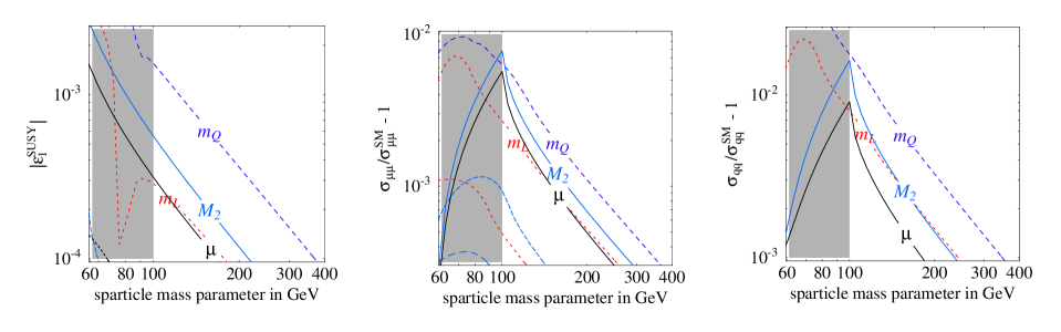
Figure 1: Corrections to $\varepsilon_{1}$ and to $\sigma(e\bar{e}\to\mu\bar{\mu},\sum_{q}q\bar{q})$ at CM energy $200\,{\rm GeV}$ generated when only the sparticle with the indicated mass is light. This allows to see the accuracy of the $\hat{S},\hat{T},W,Y$ approximation, which gives straight lines with the correct asymptotic behavior for $m_{\rm SUSY}\gg M_{Z}$.

This feature is illustrated in fig. 1, where we show full numerical results for the corrections to a few observables. We consider a variety of sparticle spectra where only one kind of sparticles is light: only left-handed sleptons, left-handed squarks, only gauginos, only Higgsinos, and so on. Their masses are respectively determined by the parameters $m_{\rm SUSY}=\{m_{L},m_{Q},\mu,M_{2},\ldots\}$. In these limits the approximation 1 (‘universal’ SUSY) becomes exact. Therefore, by making also approximation 2 (‘heavy’ SUSY), gives the correct asymptotic $1/m_{\rm SUSY}^{2}$ behavior for $m_{\rm SUSY}\gg M_{Z}$, which would correspond to straight lines in fig. 1. We see that all curves remain roughly straight in all the allowed range $m_{\rm SUSY}\,\raise 1.29167pt\hbox{$>$\kern-7.5pt\lower 4.30554pt\hbox{$\sim$}}\,100\,{\rm GeV}$. Approximation 2 badly fails only for $m_{\rm SUSY}\,\raise 1.29167pt\hbox{$<$\kern-7.5pt\lower 4.30554pt\hbox{$\sim$}}\,100\,{\rm GeV}$, which is now excluded.

Later we give some examples of the accuracy of our approximations. We skip a detailed discussion of the accuracy of approximation 1 because it is not new, and because there is no simple general way of comparing approximation 1 with full results. We remark that since the two approximations introduce comparable errors, to really improve the accuracy one needs to avoid both approximations. E.g. analyses performed dropping approximation 2 (‘heavy’ SUSY) but making the approximation 1 (‘universal’ SUSY i.e. corrections to vertices and boxes are neglected) are much more complicated than our approximate analysis, without being significantly more accurate.

We also perform a full one-loop analysis, supplementing the traditional precision data with LEP2 $e^{+}e^{-}\to e^{+}e^{-},\mu^{+}\mu^{-},\tau^{+}\tau^{-},q\bar{q}$ cross sections. Almost all needed pieces of the computations can be obtained from literature: SUSY corrections to gauge boson propagators can be found in [12, 13, 14, 1], to $Z$-boson vertices in [15, 1], to $\mu$-decay in [12, 16, 1, 13], to LEP2 $e\bar{e}\to f\bar{f}$ cross sections in [17] (only for $f\neq e$). We have recomputed all LEP2 cross sections, including for the first time $e^{+}e^{-}\to e^{+}e^{-}$, using the FeynArts, FormCalc and LoopTools codes [18, 19]. Technical details are given in appendix A.

$$\begin{array}[]{cccc}\displaystyle{\color[rgb]{0,0,0.4}\widehat{S}}=\frac{g}{g^{\prime}}\Pi^{\prime}_{W_{3}Y}(0)&\displaystyle{\color[rgb]{0,0,0.4}\widehat{T}}=\frac{\Pi_{W_{3}W_{3}}(0)-\Pi_{W^{+}W^{-}}(0)}{M_{W}^{2}}&\displaystyle\quad{\color[rgb]{0,0,0.4}W}=\frac{M_{W}^{2}}{2}\Pi^{\prime\prime}_{W_{3}W_{3}}(0)&\displaystyle{\color[rgb]{0,0,0.4}Y}=\frac{M_{W}^{2}}{2}\Pi^{\prime\prime}_{YY}(0)\\ \displaystyle\quad(H^{\dagger}\tau^{a}H)W^{a}_{\mu\nu}Y_{\mu\nu}&\displaystyle|H^{\dagger}D_{\mu}H|^{2}&\displaystyle\frac{(D_{\rho}W^{a}_{\mu\nu})^{2}}{2}&\displaystyle\frac{(\partial_{\rho}Y_{\mu\nu})^{2}}{2}\end{array}$$

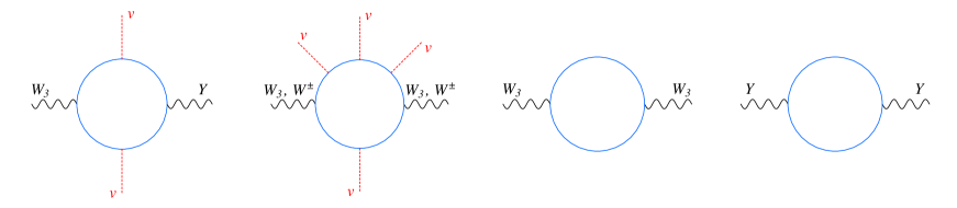
Figure 2: Upper row: definition of $\hat{S}$, $\hat{T}$, $W$ and $Y$ in terms of canonically normalized inverse propagators $\Pi$. Middle row: the corresponding dimension 6 operators. Lower row: one-loop Feynman graphs that contribute to $\hat{S}$, $\hat{T}$, $W$ and $Y$. Unspecified lines denote generic sparticles.

We now give simple analytic expressions for SUSY effects in ‘heavy universal’ approximation. We list how each sparticle contributes to $\hat{S},\hat{T},W,Y$. The contributions to $\hat{S},\hat{T},W,Y$ are obtained computing the diagrams in the lower row of fig. 2, that directly correspond to the dimension 6 operators listed in the middle row of fig. 2. Sometimes our analytic approximations have a definite sign, confirming some results previously noticed by performing numerical scans.

2.1 Sfermions

The three generations of sfermions with masses $m_{L},m_{E},m_{Q},m_{U},m_{D}$ and hypercharges

$$Y_{L}=-1/2,\;\;\;\;Y_{E}=1,\;\;\;\;Y_{Q}=1/6,\;\;\;\;Y_{U}=-2/3,\;\;\;\;Y_{D}=1/3.$$ (3)

give

$$\halign to=0.0pt{\@eqnsel\hskip\@centering$\displaystyle{#}$&\global\@eqcnt\@ne\hskip 2\arraycolsep\hfil${#}$\hfil& \global\@eqcnt\tw@\hskip 2\arraycolsep$\displaystyle{#}$\hfil&\llap{#}\cr 0.0pt plus 1000.0pt$\displaystyle{\hat{S}&10.0pt\hfil${=&10.0pt$\displaystyle{- \frac{\alpha_{2}}{24\pi} \bigg{[} M_{W}^{2}\bigg{(} 3\frac{Y_{L}}{m_{L}^{2}}+9\frac{Y_{Q}}{m_{Q}^{2}}\bigg{)}\cos 2\beta+\frac{1}{2} \frac{m_{t}^{2}}{m_{Q}^{2}}\bigg{]}, \\ \hat{T} &\hbox to0.0pt{\hss= &\frac{\alpha_{2}}{16\pi}M_{W}^{2}\cos^{2}2\beta\bigg{(}\frac{1}{m_{L}^{2}}+\frac{2}{m_{Q}^{2}}\bigg{)}+\hat{T}_{\rm stop},\\Y&=&\frac{\alpha_{Y}}{40\pi}M_{W}^{2}\bigg{(}\frac{Y_{E}^{2}}{m_{E}^{2}}+2\frac{Y_{L}^{2}}{m_{L}^{2}}+3\frac{Y_{D}^{2}}{m_{D}^{2}}+3\frac{Y_{U}^{2}}{m_{U}^{2}}+6\frac{Y_{Q}^{2}}{m_{Q}^{2}}\bigg{)},\\W&=&\frac{\alpha_{2}}{80\pi}M_{W}^{2}\bigg{(}\frac{1}{m_{L}^{2}}+\frac{3}{m_{Q}^{2}}\bigg{)}.&(4)\cr}}}}}$$

We assumed that sfermions within each generation have the same mass: $m_{L_{1}}=m_{L_{2}}=m_{L_{3}}\equiv m_{L}$ and so on. If sfermions of different generations have instead different masses our above expressions can be immediately generalized. The leading order approximation to the stop contribution,

$$\hat{T}_{\rm stop}=\frac{\alpha_{2}}{16\pi}\frac{(m_{t}+M_{W}\cos 2\beta)^{2}}{m_{Q_{3}}^{2}M_{W}^{2}}$$

is often not accurate enough, mainly because of the possibility of sizable stop mixing $\theta_{\tilde{t}}$ induced by $A_{t}$ is neglected. This effect could be taken approximatively into account, but we prefer to use the exact expression for $\hat{T}_{\rm stop}$

$$\hat{T}_{\rm stop}=\frac{3\alpha_{2}}{16\pi M_{W}^{2}}\bigg{[}\cos^{2}\theta_{\tilde{t}}\,f(m^{2}_{\tilde{t}_{1}},m^{2}_{\tilde{b}_{L}})+\sin^{2}\theta_{\tilde{t}}\,f(m^{2}_{\tilde{t}_{2}},m^{2}_{\tilde{b}_{L}})-\sin\theta_{\tilde{t}}\cos\theta_{\tilde{t}}\,f(m^{2}_{\tilde{t}_{1}},m^{2}_{\tilde{t}_{2}})\bigg{]}$$

because it is so simple that expanding it cannot give a significant simplification. In the above equations $m_{\tilde{t}_{1,2}}$ are stop masses, $f(a,b)=a+b+2ab\ln(a/b)/(b-a)$. For large $\tan\beta$ one needs to take into account also sbottom mixing.

Notice that $W,Y>0$. Furthermore $\hat{S}$ is almost always negative (the positive $Y_{Q}$ contribution is dominant only if squarks of the first two generations are enough lighter than sleptons and stops). The factor $\cos 2\beta=(v_{d}^{2}-v_{u}^{2})/v^{2}<0$ is associated to custodial symmetry breaking.

2.2 MSSM Higgs bosons

Their properties are determined, at tree level, by two parameters: $\tan\beta$ and the mass of the pseudo-scalar Higgs $m_{A}=[m_{h_{\rm u}}^{2}+m_{h_{\rm d}}^{2}+2|\mu|^{2}]^{1/2}$. We find

$$\halign to=0.0pt{\@eqnsel\hskip\@centering$\displaystyle{#}$&\global\@eqcnt\@ne\hskip 2\arraycolsep\hfil${#}$\hfil& \global\@eqcnt\tw@\hskip 2\arraycolsep$\displaystyle{#}$\hfil&\llap{#}\cr 0.0pt plus 1000.0pt$\displaystyle{\hat{S}&10.0pt\hfil${=&10.0pt$\displaystyle{-\frac{\alpha_{2}}{48\pi} \frac{M_{W}^{2}}{m_{A}^{2}}(1-\frac{M_{Z}^{2}}{2M_{W}^{2}}\sin^{2}2\beta),\\ \hat{T} &\hbox to0.0pt{\hss= &\frac{\alpha_{2}}{48\pi}\frac{M_{W}^{2}}{m_{A}^{2}}(1-\frac{M_{Z}^{2}}{M_{W}^{2}}\sin^{2}2\beta),\\Y&=&\frac{\alpha_{Y}}{240\pi}\frac{M_{W}^{2}}{m_{A}^{2}},\\W&=&\frac{\alpha_{2}}{240\pi}\frac{M_{W}^{2}}{m_{A}^{2}}.&(5)\cr}}}}}$$

The Higgs contributions to $W,Y$ are always positive, the contribution to $\hat{S}$ is negative, the contribution to $\hat{T}$ is positive for $\tan\beta\,\raise 1.29167pt\hbox{$>$\kern-7.5pt\lower 4.30554pt\hbox{$\sim$}}\,1.7$. Higgs bosons contribute to $W,Y$ in the same way as one slepton doublet with $m_{L}\leftrightarrow m_{A}$. Their contributions to $\hat{S},\hat{T}$ are instead different, because ${\rm SU}(2)_{L}$-breaking affects differently Higgs masses and slepton masses. MSSM Higgs bosons give ‘small’ corrections to $\hat{S},\hat{T},W,Y$.

2.3 Gauginos and higgsinos

Their contributions to $\hat{S},\hat{T},W,Y$ are obtained computing the diagrams in fig. 2. The resulting expressions in terms of $M_{1},M_{2},\mu,\beta$ are explicit (unlike the usual ones, written as sums over chargino and neutralino eigenstates appropriately weighted by their eigenvectors) but lengthy. Since we anyhow expect that for light sparticles our approximations are accurate within $\sim 30\%$, for simplicity we here report them neglecting terms suppressed by $s_{\rm W}^{2}\approx 0.22$. In this limit $\hat{S},\hat{T}$ no longer depend on $M_{1}$. The terms that we neglect vanish in the limit $M_{1}\gg M_{2},|\mu|$.

No further approximation is needed for $W$ and $Y$, which are given by simple expressions. Gauginos and higgsinos contribute as

$$\halign to=0.0pt{\@eqnsel\hskip\@centering$\displaystyle{#}$&\global\@eqcnt\@ne\hskip 2\arraycolsep\hfil${#}$\hfil& \global\@eqcnt\tw@\hskip 2\arraycolsep$\displaystyle{#}$\hfil&\llap{#}\cr 0.0pt plus 1000.0pt$\displaystyle{\hat{S}&10.0pt\hfil${= &10.0pt$\displaystyle{\frac{\alpha_{2} M_{W}^{2}}{12\pi M_{2}^{2}}\bigg{[} \frac{r(r-5-2r^{2})}{(r-1)^{4}}+ \frac{1-2r+9r^{2}-4r^{3}+2r^{4}}{(r-1)^{5}}\ln r \bigg{]} +\\ &\hbox to0.0pt{\hss&+\frac{\alpha_{2}M_{W}^{2}}{24\pi M_{2}\mu}\bigg{[}\frac{2-19r+20r^{2}-15r^{3}}{(r-1)^{4}}+\frac{2+3r-3r^{2}+4r^{3}}{(r-1)^{5}}2r\ln r\bigg{]}\sin 2\beta,\\\hat{T}&=&\frac{\alpha_{2}M_{W}^{2}}{48\pi M_{2}^{2}}\bigg{[}\frac{7r-29+16r^{2}}{(r-1)^{3}}+\frac{1+6r-6r^{2}}{(r-1)^{4}}6\ln r\bigg{]}\cos^{2}2\beta,\\Y&=&\frac{\alpha_{Y}}{30\pi}\frac{M_{W}^{2}}{\mu^{2}},\\W&=&\frac{\alpha_{2}}{30\pi}\bigg{[}\frac{M_{W}^{2}}{\mu^{2}}+\frac{2M_{W}^{2}}{M_{2}^{2}}\bigg{]}&(6)\cr}}}}}$$

where $r=\mu^{2}/M_{2}^{2}$. While $W$ and $Y$ are positive, $\hat{S}$ and $\hat{T}$ can have both signs. The second contribution to $\hat{S}$ is suppressed by one power of $\tan\beta$. Notice that for $|\mu|\ll M_{1},M_{2}$ or for $|\mu|\gg M_{2},M_{1}$ $\hat{S}$ and $\hat{T}$ are negligible because suppressed by the heaviest mass, while corrections to $W$ and $Y$ can still be sizable because suppressed by the lightest mass.

2.4 General features

Presently SUSY models have many unknown parameters and there is no experimental evidence for SUSY: a general analytic understanding seems more appropriate than detailed numerical analyses focussed on particular points.

All contributions to $\hat{S},\hat{T},W,Y$ are of order $(gM_{W}/4\pi m_{\rm SUSY})^{2}$, with the exception of corrections due to stops. As well known, and as clear from fig. 2, stops give corrections to $\hat{T}$ enhanced by $(\lambda_{t}/g)^{4}$ and corrections to $\hat{S}$ enhanced by $(\lambda_{t}/g)^{2}$. This is the largest single effect if $m_{Q_{3}}$ is small enough.

Otherwise the total effect can still be detectable, in view of the cumulative effect of the large number of sparticles. E.g. all sparticles give positive contributions to $W,Y$. Setting all sparticles to a common mass $m_{\rm SUSY}$ one gets $W\approx 10^{-3}({100\,{\rm GeV}}/{m_{\rm SUSY}})^{2}$. Without including LEP2, data are compatible with the SM with a mild preference for a positive $W$ (i.e. a negative correction to $\varepsilon_{2}$). This preference disappears when LEP2 is included and the measured value of $W$ disfavors at almost $2\sigma$ having all these sparticles as light as allowed by direct experimental bounds, $m_{\rm SUSY}\approx 100\,{\rm GeV}$.

One important feature of the above expressions for $\hat{S},\hat{T},W,Y$ is the absence of notable features, either suppressions or enhancements. Furthermore SUSY corrections to precision observables mainly depend on a few SUSY parameters: left-handed slepton and squark masses, $M_{2}$ and $\mu$. This makes precision data a ‘robust’ generic test, unlike other effects (like $b\to s\gamma$, $g_{\mu}-2$, $B_{s}\to\mu\bar{\mu}$) which can be strongly enhanced in some regions of the parameter space (e.g. at large $\tan\beta$) and negligible in other regions (e.g. in the ‘split’ SUSY limit [7]). Another example is the predicted abundancy of thermal dark matter, which is suppressed in corners of the parameter space where the two lightest sparticles happen to be quasi-degenerate [20].

Furthermore corrections to precision observables are ‘robust’ under variations of the SUSY model. E.g. the non-observation of the lightest Higgs might be interpreted as an effect of some extra physics that increases the MSSM prediction for the Higgs mass. The simplest option is adding a singlet chiral superfield coupled to the Higgs doublets. Such extra singlet can drastically affect also dark matter signals of SUSY, but has almost no impact on precision tests.

We will consider several models, showing contours in the $(m_{0},M_{1/2})$ plane (in the CMSSM, and analogous ones in other models) with the $\mu$ parameter determined from the condition of correct electroweak symmetry breaking. This kind of plots hides the fact that most of the SUSY parameter space stays at light $m_{0},M_{1/2},\ldots\sim M_{Z}$, and that actually most of the parameter space has already been excluded [21]. We are interested in SUSY as long as it solves the hierarchy problem: therefore we restrict our analysis to sparticle spectra reasonably close to the weak scale.

As usual this is just a two parameter slicing: models have more free parameters (e.g. $\tan\beta$, $A$-terms, sign of $\mu$,…) which are kept fixed at arbitrarily chosen values. While this is often a critical arbitrary choice, precision data are again ‘robust’: i.e. we will find smooth feature-less contours that are rather insensitive to values of the extra parameters. Therefore we will show a small number of figures.

      

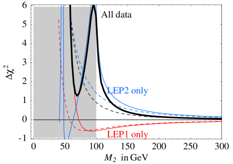
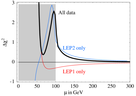
Figure 3: Fig. 3a: $\chi^{2}-\chi^{2}_{\rm SM}$ in the case of light gauginos with $\tan\beta=10$, gaugino unification and $m_{h}=115\,{\rm GeV}$. The dashed line are our analytical approximation, while the continuous lines are the full numerical computation. The thick line is the result obtained including all data. The upper blue line shows the contribution of LEP2 only. The lower red line shows the result omitting LEP2, including only ‘traditional’ precision data. The shaded regions is excluded by direct LEP2 searches. Fig. 3b: analogous plot for the case of light higgsinos. We show only the full result.

3 ‘Split’ supersymmetry

We start with a simple case: we assume that only fermionic sparticles are light so that only corrections to propagators are relevant. This might be not only a warming exercise: the MSSM with heavy scalar sparticles received recent attention [7]. In this limit most MSSM problems get milder, most MSSM successes are retained but SUSY no longer solves the hierarchy ‘problem’. This was considered as the most important success of SUSY, but alternative antrophic interpretations [23, 24] gained credit in view of recent results: the possible discovery of a small cosmological constant; the non-observation of new physics around the Fermi scale; the realization that string models are even more abundant that what feared. This anthropic scenario is pudically named ‘split supersymmetry’.

Although there is no longer a link between the scales of SUSY breaking and of electroweak symmetry breaking, we still restrict our attention to fermionic sparticles close to the Fermi scale, because only in this case precision observables receive detectable corrections. In the same way, scalar sparticles give negligible effects even if they are relatively close to the Fermi scale, so that SUSY can still solve the hierarchy problem.

The spectrum of fermionic sparticles is specified by $\mu,M_{1},M_{2},M_{3}$ and $\tan\beta$. We assume a GUT relation among gaugino masses, $\tan\beta=10$ and $m_{h}=115\,{\rm GeV}$.

Let us start from the sub-case in which only gaugino masses are around $M_{Z}$ and all other sparticles are much heavier. In $\hat{S},\hat{T},W,Y$ approximation we have

$$\hat{S}=\hat{T}=Y\simeq 0,\qquad W\simeq\frac{\alpha_{2}}{15\pi}\frac{M_{W}^{2}}{M_{2}^{2}}$$ (7)

which does not depend on $\tan\beta,M_{1},M_{3}$. Fitting only traditional precision data (LEP1, SLD, the $W$ mass,…) gives $W=(0.7\pm 0.9)\cdot 10^{-3}$ i.e. a almost $1\sigma$ preference for $M_{2}\approx 80\,{\rm GeV}$, as emphasized in [3] (see also [1]). Adding LEP2 data this preference disappears because the best fit shifts towards negative $W$. Going beyond the $\hat{S},\hat{T},W,Y$ approximation, this result is confirmed by the exact numerical result, shown in fig. 3a. We see that in all the experimentally allowed range for the chargino mass, $M_{\chi}\,\raise 1.29167pt\hbox{$>$\kern-7.5pt\lower 4.30554pt\hbox{$\sim$}}\,100\,{\rm GeV}$, the $\hat{S},\hat{T},W,Y$ approximation accurately reproduces the full LEP1 fit. On the contrary when the lightest chargino or neutralino is slightly above the LEP2 direct limit, $M_{\chi}\approx 100\,{\rm GeV}$, the $\hat{S},\hat{T},W,Y$ approximation underestimates SUSY corrections to LEP2 observables, because one loop chargino and neutralino corrections to LEP2 observables are enhanced by an ${\cal O}(1)$ factor, by having a virtual chargino or neutralino almost on-shell. Going to chargino and neutralino masses above the LEP2 direct bound the resonant enhancement disappears and the $\hat{S},\hat{T},W,Y$ approximation becomes correct.

The same thing happens if only higgsinos are light: in this limit

$$\hat{S}=\hat{T}\simeq 0,\qquad W\simeq Y\simeq\frac{\alpha_{2}}{30\pi}\frac{M_{W}^{2}}{\mu^{2}}.$$ (8)

Ignoring LEP2 we agree with [3]; including LEP2 we get the different result of fig. 3b.

Finally, fig. 5a shows the global fit of precision data in the ($M_{2},\mu$) plane. We find no favored regions, nor new statistically significant constraints. Gauginos and higgsinos masses slightly above their bound from direct searches are mildly disfavored by precision data. For comparison fig. 6a shows the global fit omitting precision LEP2 data. Notice that in the ‘split’ SUSY limit there are no corrections to $g_{\mu}-2$, $b\to s\gamma$,….

      

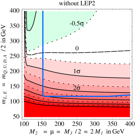
Figure 4: Fit of precision data with the sample sparticle spectrum of eq. (9). The label ‘$3\sigma$’ means $\Delta\chi^{2}=3^{2}$ (i.e. SUSY is disfavoured) and the label ‘$-0.5\sigma$’ means $\Delta\chi^{2}=-0.5^{2}$ (i.e. SUSY is favoured).

4 A simple sparticle spectrum

Before considering popular models, we compare data with a simple sparticle spectrum, chosen such that all sparticles can be at the same time close to present direct collider bounds. We assume

$$m_{E}=m_{L}=m_{Q}/2=m_{U}/2=m_{D}/2=m_{A}/2,\qquad M_{2}=\mu=2M_{1}=M_{3}/2,\qquad\tan\beta=10$$ (9)

and vanishing $A$-terms. All parameters are renormalized at the weak scale. The gluino mass $M_{3}$ marginally affects precision data, and could increased in order to avoid constraints from hadron colliders. The result is shown in fig. 4a (LEP2 data included) and in fig. 4b (LEP2 not included). Here and in the following, we plot iso-lines of $\Delta\chi^{2}=\chi^{2}-\chi^{2}_{\rm SM}$. Below the thick line some charged sparticle is lighter than $100\,{\rm GeV}$, which is excluded by direct searches at LEP2. We see that precision data disfavor regions where all sparticles are close to present direct bounds. In the next sections we analyze popular models, finding analogous results. Constraints will be somewhat weaker because such models force colored sparticles and Higgsinos to be heavier than what allowed by direct searches.

LEP2 precision data included

      

      

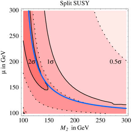
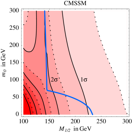
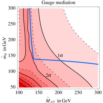
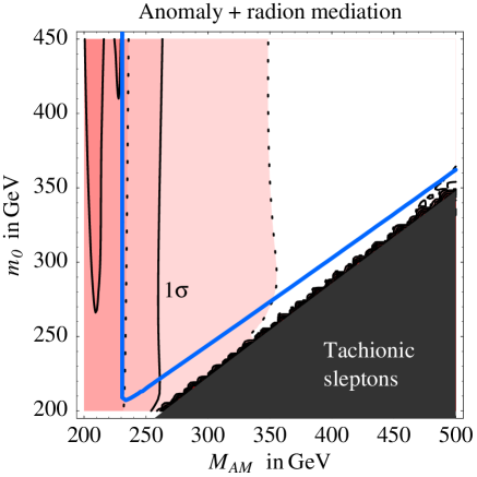
Figure 5: Fits of precision data. Regions shaded in red are disfavored at $1,2,3,\ldots\sigma$, as indicated on the iso-lines. Regions below the thick blue line are excluded by LEP2 direct searches. We performed a full one-loop analysis, including LEP2 precision data. We kept fixed $\tan\beta=10$, $A_{0}=0$, $\lambda_{t}(M_{\rm GUT})=0.6$, $\hbox{\rm sign}\,\mu=+1$, the gauge-mediation scale $M_{\rm GM}=10^{10}\,{\rm GeV}$.

LEP2 precision data not included

      

      

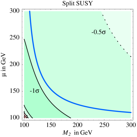
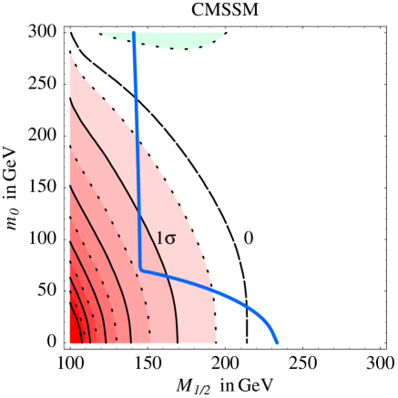
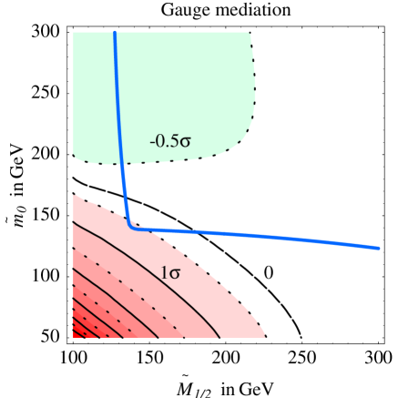
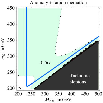
Figure 6: As in fig. 5, but without including LEP2 precision data. Regions shaded in green are favored at $-1,2,3,\ldots\sigma$.

5 CMSSM

Unification of gauge couplings and the non-observation of SUSY flavor effects suggests the following assumption about the sparticle spectrum renormalized at the GUT scale $M_{\rm GUT}\approx 2~{}10^{16}\,{\rm GeV}$:

$$M_{1,2,3}=M_{1/2},\qquad m_{L,Q,U,D,E,H_{\rm u},H_{\rm d}}^{2}=m_{0}^{2},\qquad A_{\rm e,d,u}=A_{0}.$$ (10)

We assume $A_{0}=0$, $\tan\beta=10$, $\mu>0$, $\lambda_{t}(M_{\rm GUT})=0.6$ (as explained in [22]). RGE running generates non vanishing $A$-terms at the weak scale. Table 1 lists the values of the low-energy parameters most important for precision observables. Fig. 5b shows the result of the global fit of precision data, including LEP2 precision data. For comparison, fig. 6b shows the analogous fit omitting LEP2 data: again there were favored regions with $M_{2}\sim M_{Z}$ and/or $|\mu|\sim M_{Z}$.

We do not show constraints from $b\to s\gamma$, $g_{\mu}-2$, $B_{s}\to\mu\bar{\mu}$, thermal Dark Matter (DM) abundancy and $m_{h}$, which unlike precision data depend significantly on other parameters ($\tan\beta$, $A_{0}$,…) kept fixed at arbitrary values. Depending on the precise value of $m_{t}$, at multi-TeV $m_{0}$ there can be a fine-tuned region with the atypical phenomenology of higgsino Lightest Supersymmetric Particle (LSP). We ignore this possibility, as higgsino LSP can be better studied in contexts where $\mu$ is naturally small, rather than fine-tuning the CMSSM in order to avoid its typical outcome, $M_{1}<|\mu|$.

We now give an example of the accuracy of the $\hat{S},\hat{T},W,Y$ approximation by considering at one specific point the three $\varepsilon_{1,2,3}$ observables. Since SUSY is not universal, we focus on three ‘leptonic’ observables, $\varepsilon_{1,2,3}^{\rm lept}$. These are defined like the usual $\varepsilon_{1,2,3}$ [11], except that $Z$-couplings are extracted only from charged lepton data (chosen because they are more precisely measured than data about neutrinos and quarks). This means that we take into account SUSY corrections to $Z,\gamma$ and $W^{\pm}$ propagators, to $Z$/charged lepton vertices, and to $\mu$-decay. The specific CMSSM point is chosen such that the thermal LSP abundancy agrees with the DM abundancy [25] (without invoking co-annihilations [20]) and such that sparticles are as light as possible. The point is $m_{0}=100\,{\rm GeV}$, $M_{1/2}=150\,{\rm GeV}$, $A_{0}=0$, $\tan\beta=10$. EW breaking is achieved for $\mu=250\,{\rm GeV}$, and the masses of the lightest neutralino, chargino and slepton are $58\,{\rm GeV}$, $105\,{\rm GeV}$, $124\,{\rm GeV}$ respectively. This point is far from all limits in which the $\hat{S},\hat{T},W,Y$ approximation becomes exact. The SUSY corrections to the $\varepsilon_{1,2,3}$ observables are

$$\begin{array}[]{lccc}&1000\,\delta\varepsilon_{1}^{\rm lept}&1000\,\delta\varepsilon_{2}^{\rm lept}&1000\,\delta\varepsilon_{3}^{\rm lept}\\ \hbox{$\hat{S},\hat{T},W,Y$ approximation:}&+0.29&-0.40&-0.43\phantom{.}\\ \hbox{Full numerical result:}&+0.36&-0.30&-0.56.\end{array}$$ (11)

$$\begin{array}[]{c|ccc}&\hbox{CMSSM}&\hbox{Gauge mediation at $10^{10}\,{\rm GeV}$}&\hbox{Anomaly + radion mediation}\\ \hline\cr M_{2}&0.82M_{1/2}&0.82\tilde{M}_{1/2}^{\phantom{X^{X}}}&-0.43M_{\rm AM}\\ m_{Q}^{2}&m_{0}^{2}+6.2M_{1/2}^{2}&6.5\tilde{m}_{0}^{2}+5.2\tilde{M}_{1/2}^{2}&m_{0}^{2}+16M_{\rm AM}^{2}\\ m_{L}^{2}&m_{0}^{2}+0.52M_{1/2}^{2}&1.3\tilde{m}_{0}^{2}+0.24\tilde{M}_{1/2}^{2}&m_{0}^{2}-0.37M_{\rm AM}^{2}\\ \mu^{2}+M_{Z}^{2}/2&0.17m_{0}^{2}+2.6M_{1/2}^{2}&2.9\tilde{m}_{0}^{2}+1.7\tilde{M}_{1/2}^{2}&0.17m_{0}^{2}+10M_{\rm AM}^{2}\end{array}$$

Table 1: Values of the low-energy parameters most important for determining SUSY corrections to precision data in the models under study.

6 Gauge mediation

Soft terms renormalized around the unknown gauge-mediation scale $M_{\rm GM}$ are predicted as [8]

$$M_{i}=\frac{\alpha_{i}}{\alpha}\tilde{M}_{1/2},\qquad m_{R}^{2}=\frac{c_{R}^{i}M_{i}^{2}}{\sqrt{n}}$$ (12)

where $\tilde{M}_{1/2}$ is a free parameter, $i=\{1,2,3\}$, $c^{i}_{R}$ are quadratic Casimir coefficients for the various representations $R$, $n$ is a free parameter equal to $n=n_{5}+3n_{10}$ in models where a single gauge singlet couples supersymmetry breaking to $n_{5}$ copies of messenger fields in the $5\oplus\bar{5}$ representation of SU(5) and to $n_{10}$ copies in the $10\oplus\overline{10}$ representation [8]. We re-parameterize it as $1/\sqrt{n}=(\tilde{m}_{0}/\tilde{M}_{1/2})^{2}$, such that $\tilde{m}_{0}$ is a ‘scalar mass parameter’ analogous to the parameter $m_{0}$ of CMSSM. In this way gauge-mediated spectra are described by two free parameters $(\tilde{m}_{0},\tilde{M}_{1/2})$ analogous to the $(m_{0},M_{1/2})$ parameters of the CMSSM. The resulting spectrum is qualitatively similar to the CMSSM (for a comparison see e.g. [26]).

We assume $\tan\beta=10$, $\lambda_{t}(M_{\rm GUT})=0.6$, $\mu>0$ and an intermediate value of the gauge-mediation scale: $M_{\rm GM}=10^{10}\,{\rm GeV}$. Table 1 list the values of the low-energy parameters most important for precision observables. The result of our full analysis is shown in fig. 5c. For comparison, fig. 6c shows the analogous fit omitting LEP2 data.

7 Anomaly and radion mediation

Generic supergravity mediation of SUSY breaking does not give the flavour-universal sfermion masses suggested by experimental constraints. A universal scalar mass $m_{0}$ can be obtained in particular situations where some particular supergravity contributions become dominant. This happens in extra dimensional models with localized fields: if MSSM fields are separated from SUSY-breaking fields by a large enough extra-dimensional distance the unwanted generic supergravity effects are forbidden by locality. Low energy supergravity gives the dominant effects, which are flavour universal and computable. One effect is anomaly mediation [9], which predicts

$$M_{i}=b_{i}g_{i}^{2}M,\qquad m_{R}^{2}=-b_{i}c_{i}^{R}g_{i}^{2}M^{2}\qquad\hbox{at any scale}$$

(we do not write predictions for $A$-terms nor for sparticles involved in the top Yukawa coupling) where $b_{1,2,3}=\{33/5,1,-3\}$ are the $\beta$-function coefficients of the MSSM gauge couplings. Sleptons have negative squared masses so that pure anomaly mediation is ruled out.

One-loop supergravity corrections give another effect: a universal contribution $m_{0}^{2}$ to scalar masses. While in the simplest situations $m_{0}^{2}<0$ [27], in some particular cases the radion-mediated contribution gives a positive $m_{0}^{2}$ [10]. Therefore models with anomaly plus radion-mediated SUSY breaking can give an acceptable sparticle spectrum:

$$M_{i}=b_{i}g_{i}^{2}M_{\rm AM},\qquad m_{R}^{2}=m_{0}^{2}-b_{i}c_{i}^{R}g_{i}^{2}M_{\rm AM}^{2}.$$ (13)

We assume that this boundary condition holds at the GUT scale and that $\tan\beta=10$ and $\mu>0$. Table 1 list the values of the low-energy parameters most important for precision observables. To a good approximation only sleptons and winos are light and can give significant effects. The result of our full analysis is shown in fig. 5d. For comparison, fig. 6d shows the analogous fit omitting LEP2 data.

8 Conclusions

We studied the corrections to precision data generated by one-loop supersymmetric effects. We performed a full analysis of propagator, vertex and box corrections. We also developed a simple understanding, based on the ‘heavy universal’ approximation, and discussed its accuracy. In this approximation all SUSY corrections to $Z$-pole, low energy and LEP2 observables are encoded in four $\hat{S},\hat{T},W,Y$ parameters: eq.s (3,2.2,2.3) give their explicit analytic expressions.

Furthermore we added for the first time LEP2 $e\bar{e}\to f\bar{f}$ cross sections to the data-set. In the global fit LEP2 data have a weight comparable to $Z$-pole data, already included in previous analyses. Hints for supersymmetry emphasized in some previous analyses [1, 2, 3] had a marginal statistical significance, and are thereby significantly affected by the inclusion of LEP2 data. Actually such hints get mostly removed, because SUSY gives positive corrections to $W,Y$ (i.e. reduce LEP2 cross sections), while LEP2 data favor $W<0$. Rather than performing a general scan searching for more fluctuating hints, we preferred to analyze specific models: ‘split’ SUSY, the CMSSM, gauge mediation and anomaly plus radion mediation.

The analytic approximation shows that SUSY corrections to precision observables mainly depend on a few SUSY parameters: left-handed slepton and squark masses, $M_{2}$ and $\mu$. (A large stop mixing and a small $\tan\beta$ would also play a significant rôle). No big enhancements or suppressions are possible, unlike in the cases of other indirect tests ($g_{\mu}-2$, $b\to s\gamma$, $B_{s}\to\mu\bar{\mu}$, dark-matter abundancy, …). Therefore by varying 2 main parameters (such as $m_{0}$ and $M_{1/2}$) keeping fixed all other parameters we produced plots which represent the general situation in a given model, rather than being only sample slices of a vast parameter space. For the same reasons such plots do not show peculiar features. In ‘split’ SUSY the only light sparticles are gauginos and higgsinos . In anomaly mediation the lightest sparticles that give the main corrections to precision observables are gauginos and sleptons. In CMSSM and gauge mediation also stops play a significant rôle. The relevance of LEP2 is clearly seen by comparing our full results of fig. 5 with fig. 6, where LEP2 is not included. We also analyzed a model where all sparticles can be as light as allowed by direct constraints: fig. 4 shows that this case is disfavored by precision data.

Acknowledgments

We thank G. Altarelli, P. Gambino, G. Giudice and R. Rattazzi for useful discussions. The research of G.M. is supported by the USA Department of Energy, under contract W-7405-ENG-36. A.S. thanks T. Hahn for help in installing the LoopTools code [19].

Appendix A Technical details

One-loop computations of LEP2 cross sections have been performed using the FeynArts and FormCalc codes [18]. Loop functions have been computed using the LoopTools code [19]. The set of data we fit is basically the same as in [6]. We compute LEP2 cross sections at the various energies around $200\,{\rm GeV}$ corresponding to the LEP2 runs.

Our full analysis of LEP1 data is performed following the lines of [11], while our full analysis of LEP2 data is performed following the lines of [17]. Unfortunately these two strategies employ different renormalization procedures, so that care is needed to combine the two analyses. The basic difference is that [11] fixes the three basic SM parameters $v,g,g^{\prime}$ using the three observables $\alpha,M_{Z},G_{\rm F}$, while [17] employs the alternative set $\alpha,M_{Z},M_{W}$. As described in [28] the second procedure is implemented by subtracting gauge boson propagators as

$$\halign to=0.0pt{\@eqnsel\hskip\@centering$\displaystyle{#}$&\global\@eqcnt\@ne\hskip 2\arraycolsep\hfil${#}$\hfil& \global\@eqcnt\tw@\hskip 2\arraycolsep$\displaystyle{#}$\hfil&\llap{#}\cr 0.0pt plus 1000.0pt$\displaystyle{\Pi_{WW}^{\rm ren}(p^{2}) &10.0pt\hfil${=&10.0pt$\displaystyle{\Pi_{WW}(p^{2}) -\Pi_{WW}(M_{W}^{2}) - (p^{2}-M_{W}^{2})\Pi'(M_{W}^{2})\\ \Pi_{ZZ}^{\rm ren}(p^{2}) &\hbox to0.0pt{\hss=&\Pi_{ZZ}(p^{2})-\Pi_{ZZ}(M_{Z}^{2})-(p^{2}-M_{Z}^{2})\Pi^{\prime}(M_{Z}^{2})\\\Pi_{AA}^{\rm ren}(p^{2})&=&\Pi_{AA}(p^{2})-\Pi_{AA}(0)-p^{2}\Pi^{\prime}_{AA}(0)\\\Pi_{AZ}^{\rm ren}(p^{2})&=&\Pi_{AZ}(p^{2})-\Pi_{AZ}(0)-p^{2}[\Pi_{AZ}(M_{Z}^{2})-\Pi_{AZ}(0)]/M_{Z}^{2}&(14)\cr}}}}}$$

such that $\alpha,M_{Z},M_{W}$ keep their tree level values.

In order to perform a global fit one has to match the two different strategies. We convert LEP2 observables, computed using the $\alpha,M_{Z},M_{W}$ scheme [17], to the $\alpha,M_{Z},G_{\rm F}$ scheme. Since LEP2 $e\bar{e}\to f\bar{f}$ cross sections do not directly depend on $M_{W}$, the only difference amounts to a shift in the values of the $Z$-couplings, as predicted in terms of the chosen set of basic observables. In both schemes $Z$-couplings are conveniently parameterized by an auxiliary effective weak angle, defined as

$$s_{\rm W}(\alpha,M_{Z},G_{\rm F})\equiv\frac{1}{2}\left[1-\sqrt{1-\frac{4\pi\alpha}{\sqrt{2}G_{F}M_{Z}^{2}}}\right],\qquad s_{\rm W}(\alpha,M_{Z},M_{W})\equiv\sqrt{1-\frac{M_{W}^{2}}{M_{Z}^{2}}}.$$ (15)

At tree level these two definitions are equivalent, while at one-loop order they differ by

$$\delta s_{\rm W}^{2}\equiv s_{\rm W}^{2}(\alpha,M_{Z},M_{W})-s_{\rm W}^{2}(\alpha,M_{Z},G_{\rm F})=2s_{\rm W}^{2}c_{\rm W}^{2}\bigg{[}\frac{\varepsilon_{3}-\varepsilon_{1}c_{\rm W}^{2}/2s_{\rm W}^{2}}{c_{\rm W}^{2}-s_{\rm W}^{2}}+\frac{\varepsilon_{2}}{2s_{\rm W}^{2}}\bigg{]}.$$ (16)

One-loop predictions for LEP2 observables $\sigma$ are then converted as

$$\sigma(\alpha,M_{Z},G_{\rm F})=\sigma(\alpha,M_{Z},M_{W})-\frac{\partial\sigma}{\partial s_{\rm W}^{2}}\delta s_{\rm W}^{2}.$$ (17)

References

- [1] G.C. Cho and K. Hagiwara, Nucl. Phys. B574 (2000) 623. O. Lebedev and W. Loinaz, hep-ph/0106056.
- [2] G. Altarelli, F. Caravaglios, G. F. Giudice, P. Gambino and G. Ridolfi, JHEP 0106 (2001) 018 [hep-ph/0106029].
- [3] S.P. Martin, K. Tobe, J.D. Wells, hep-ph/0412424.
- [4] ALEPH, DELPHI, L3, OPAL collaborations and LEP, SLD electroweak working groups, hep-ex/0412015. The LEP2 data we fitted are summarized and combined in its chapter 8. See also, the LEP electroweak working group, web page www.web.cern.ch/LEPEWWG. We include the recent average of the top mass from the CDF and D0 collaborations and Tevatron electroweak working group, hep-ex/0404010. The NuTeV collaboration, Phys. Rev. Lett. 88 (2002) 091802. M. Kuchiev and V. Flambaum, hep/0305053. The SLAC E158 collaboration, hep-ex/0312035 and hep-ex/0403010.
- [5] For the differential cross sections we use instead the most recent results presented in: OPAL collaboration, CERN-EP/2003-053 and in: ALEPH collaboration, “Fermion Pair production in e+e- collisions at 189-209 GeV and Constraints on Physics Beyond the Standard Model”, paper in preparation.
- [6] R. Barbieri, A. Pomarol, R. Rattazzi and A. Strumia, Nucl. Phys. B 703 (2004) 127 [hep-ph/0405040].
- [7] See e.g. N. Arkani-Hamed, S. Dimopoulos, G. F. Giudice and A. Romanino, hep-ph/0409232 and ref.s therein.
- [8] L. Alvarez-Gaume, M. Claudson and M.B. Wise, Nucl. Phys. B207 (1982) 96. M. Dine and W. Fishler, Nucl. Phys. B204 (1982) 346.
- [9] L. Randall and R. Sundrum, Nucl. Phys. B557, 79 (1999) [hep-th/9810155]. G. F. Giudice, M. A. Luty, H. Murayama and R. Rattazzi, JHEP 12, 027 (1998) [hep-ph/9810442].
- [10] R. Rattazzi, C. A. Scrucca, and A. Strumia, Nucl. Phys. B674, 171 (2003) [hep-th/0305184]. T. Gregoire et al., hep-th/041121.
- [11] G. Altarelli and R. Barbieri, Phys. Lett. B 253 (1991) 161. G. Altarelli, R. Barbieri and F. Caravaglios, Phys. Lett. B 314 (1993) 357.
- [12] J.A. Grifols and J. Sola, Phys. Lett. 137B, 257 (1984); ibid. Nucl. Phys. B253, 47 (1985).
- [13] D.M. Pierce, J.A. Bagger, K.T. Matchev, R.J. Zhang, Phys. Rev. D55 (1997) 3188 [hep-ph/9606211].
- [14] P.H. Chankowski, S. Pokorski and J. Rosiek, Nucl. Phys. B423, 437 (1994).
- [15] Kane et al., hep-ph/9408228. P.H. Chankowski, S. Pokorski, hep-ph/9603310. A. Dedes, A.B. Lahanas, K. Tamvakis, hep-ph/9801425.
- [16] P.H. Chankowski, A. Dabelstein, W. Hollik, W.M. Mösle, S. Pokorski and J. Rosiek, Nucl. Phys. B417, 101 (1994).
- [17] W. Hollik and C. Schappacher, Nucl. Phys. B 545 (1999) 98 [hep-ph/9807427].
- [18] T. Hahn, Comput. Phys. Commun. 140 (2001) 418 [hep-ph/0012260]. T. Hahn and C. Schappacher, Comput. Phys. Commun. 143 (2002) 54 [hep-ph/0105349]. T. Hahn and M. Perez-Victoria, Comput. Phys. Commun. 118 (1999) 153 [hep-ph/9807565]. T. Hahn, hep-ph/0406288.
- [19] G. Passarino and M. J. G. Veltman, Nucl. Phys. B 160, 151 (1979). Passarino-Veltman functions are partly computed using the code LoopTools, available at www.feynarts.de/looptools and described in T. Hahn, Nucl. Phys. Proc. Suppl. 89 (2000) 231 [hep-ph/0005029].
- [20] K. Griest and D. Seckel, Phys. Rev. D 43 (1991) 3191. J. R. Ellis, T. Falk, K. A. Olive and M. Srednicki, Astropart. Phys. 13 (2000) 181 [Erratum-ibid. 15 (2001) 413]. T. Nihei, L. Roszkowski and R. Ruiz de Austri, JHEP 0207 (2002) 024.
- [21] L. Giusti, A. Romanino and A. Strumia, Nucl. Phys. B 550 (1999) 3 [hep-ph/9811386].
- [22] A. Romanino and A. Strumia, Phys. Lett. B 487 (2000) 165 [hep-ph/9912301].
- [23] S. Weinberg, Phys. Rev. Lett. 59 (1987) 2607.
- [24] V. Agrawal, S. M. Barr, J. F. Donoghue and D. Seckel, Phys. Rev. D 57 (1998) 5480 [hep-ph/9707380].
- [25] See e.g. J. R. Ellis, K. A. Olive, Y. Santoso and V. C. Spanos, Phys. Lett. B 565 (2003) 176.
- [26] A. Strumia, Phys. Lett. B 409 (1997) 213 [hep-ph/9705306].
- [27] T. Gherghetta and A. Riotto, Nucl. Phys. B623, 97 (2002). I. L. Buchbinder et al., Phys. Rev. D70, 025008 (2004).
- [28] A. Denner, Fortsch. Phys. 41 (1993) 307.