Probing the absolute density of the Earth’s core using a neutrino beam

Abstract

We demonstrate that one could measure the absolute matter density of the Earth’s core with a vertical neutrino factory baseline at the per cent level for $\sin^{2}2\theta_{13}\gtrsim 0.01$, where we include all correlations with the oscillation parameters in the analysis. We discuss the geographical feasibility of such an approach, and illustrate how the results change as a function of the detector location. We point out the complementarity to geophysics.

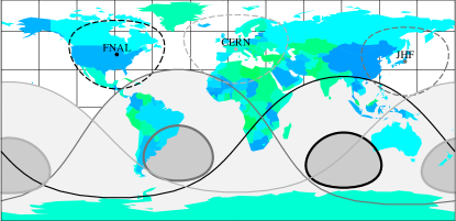
Figure 1: (Color online) Positions of three of the major potential neutrino factory laboratories, (typical) $L=3\,000\,\mathrm{km}$ detector sites (dashed curves), as well as potential detector sites with outer core crossing baselines (below thin solid curves), and inner core crossing baselines (within thick solid curves). The colors of the curves represent the different laboratories.

Neutrino oscillation physics has entered the age of precision physics, which means that the leading atmospheric and solar oscillation parameters are known to high precisions and the next generation of long-baseline experiments will be highly sensitive to sub-leading effects. These long-baseline experiments send an artificially produced neutrino beam of energy $E$ on a straight baseline (length $L$) through the Earth to a detector, which is, depending on the neutrino energy, several hundred to many thousand kilometers away. In particular, the future potential high precision instrument “neutrino factory” Geer:1998iz leads to typical baselines $\sim 700\,\mathrm{km}-7\,500\,\mathrm{km}$ relevant for neutrino oscillation physics. It is an interesting feature of neutrino oscillations that the flavor conversion is sensitive to the electron density $n_{e}$ of Earth matter Wolfenstein:1978ue , which has been suggested to be used for neutrino oscillation tomography of the Earth’s interior Ermilova:1988pw ; Ohlsson:2001ck ; Lindner:2002wm . The electron density then translates into the matter density by $\rho=n_{e}\,m_{N}/Y_{e}$ with $Y_{e}=Z/A$ the “electron fraction” and $m_{N}$ the nucleon mass. For a neutrino factory, the signal amplitude of such a measurement using the flavor conversion $\nu_{\mu}\leftrightarrow\nu_{e}$ is given by the parameter $\sin^{2}2\theta_{13}$, which has so far only been constrained by the CHOOZ experiment to $\sin^{2}2\theta_{13}\lesssim 0.1$ Apollonio:1999ae . Future long baseline experiments will find $\sin^{2}2\theta_{13}>0$ within the coming ten years if $\sin^{2}2\theta_{13}\gtrsim 0.01$ (see, e.g., LABEL:~Huber:2004ug ).

The most successful approach to the tomography of the Earth’s interior has been seismic wave geophysics primarily using seismic waves from earthquakes to reconstruct a profile of the Earth’s interior. Most of the energy produced by an earthquake is deposited in shear waves (s-waves), which cannot penetrate into the Earth’s (outer) liquid core (but might be partially converted into p-waves). A smaller fraction of energy goes into pressure waves (p-waves), which are propagated into the Earth’s core, too. The waves are partially reflected at the mantle-outer core and outer core-inner core boundaries. Therefore, seismic waves are highly sensitive to density jumps and the positions of these boundaries. Seismic waves geophysics leads to a propagation velocity profile of the Earth’s interior, which can be translated into a density profile with the equation of state. This conversion is based on a model for the shear/bulk modulus, which implies uncertainties. In fact, the most direct information on the matter density distribution comes from the Earth’s mass and its moment of inertia about the polar axis, which are, however, not uniquely determining it. In particular, there are many open questions about the Earth’s inner core (see, e.g., LABEL:~Steinle-Neumann:2002 ). Therefore, a measurement of the absolute electron density of the Earth’s core could provide very complementary information to geophysics.

From the point of view of a neutrino factory, this would require a “vertical” baseline, i.e., a decay tunnel which is vertical. Since there are only a number major high energy laboratories which are candidates for a neutrino factory, all of these on the northern hemisphere, the geographical aspect is another important part of this problem. As it is illustrated in Fig. 1, there are indeed possible detector locations (i.e., on land instead of in water) for many of the major laboratories with core crossing baselines. For example, a baseline from CERN to New Zealand crosses the inner core of the Earth.

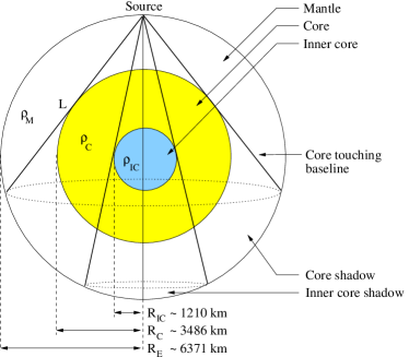
Figure 2: (Color online) The geometry of the core tomography problem (not to scale).

The geometry and the quantities of interest of the Earth tomography problem are illustrated in Fig. 2. Though neutrino oscillations are, in principle, sensitive to structural features of the density profile, realistic experiments with only one baseline have only very limited abilities for a detailed reconstruction because they are insensitive to structures much shorter than the oscillation length in matter Ohlsson:2001ck . Therefore, it is important that the relevant independent parameters be identified. In particular, treating the (average) outer and inner core densities $\rho_{C}$ and $\rho_{IC}$ as independent parameters (cf., Fig. 2) implies strong correlations Lindner:2002wm . However, these two quantities are not really independent, since the total mass of the Earth is extremely well known. In addition, we have very good knowledge on the Earth’s mantle from seismic wave geophysics. If we furthermore assume that the positions of the mantle-outer core and outer core-inner core boundaries are very well known from the reflections of seismic waves, we can reduce the number of parameters to one (either $\rho_{C}$ or $\rho_{IC}$). Below, we will argue that it is always reasonable to measure the average density of the “innermost” shell a baselines crosses.

Neutrino oscillations are, for the slowly enough varying matter density within each shell $\rho_{i}$ (mantle, outer core, or inner core), to a first approximation determined by the baseline averaged density $\bar{\rho}^{L}_{i}=1/L\int_{0}^{L}\tilde{\rho}(l)dl$ Ohlsson:2001et . Here $\tilde{\rho}(l)$ is the density along the baseline. On the other hand, the average density of the Earth is determined by the volume averaged density, which is, for each shell, given by $\bar{\rho}^{V}_{i}=4\pi/V\int_{R_{1}}^{R_{2}}\rho(r)r^{2}dr$. Here $r$ is the distance from the Earth’s center and $V=4/3(R_{2}^{3}-R_{1}^{3})\pi$ the volume of the shell. This means that the density within each differential shell $dr$ is weighted with $r^{2}$. For the total mean density of the Earth we then have

$$\bar{\rho}^{V}=(\bar{\rho}^{V}_{IC}-\bar{\rho}^{V}_{C})\left(\frac{R_{IC}}{R_{E}}\right)^{3}+(\bar{\rho}^{V}_{C}-\bar{\rho}^{V}_{M})\left(\frac{R_{C}}{R_{E}}\right)^{3}+\bar{\rho}^{V}_{M}$$

The constraint $M_{E}=const$, i.e., $\bar{\rho}^{V}=const$ because of the (approximately) known volume, together with the assumption of a known/fixed $\bar{\rho}^{V}_{M}$, leads by differentiation with respect to $\bar{\rho}^{V}_{IC}$ to $\Delta\bar{\rho}^{V}_{C}=-\left(R_{IC}/R_{C}\right)^{3}\,\Delta\bar{\rho}^{V}_{IC}\simeq-0.04\,\Delta\bar{\rho}_{IC}$. Thus, a large change in the measurement in $\bar{\rho}^{V}_{IC}$ can be compensated by a very small change in $\bar{\rho}^{V}_{C}$ because of the volume averaging. The same is, in principle, true for the outer core and mantle densities. Since the effect on neutrino oscillations is proportional to the baseline length within each shell and not to the volume, each shell contributes to the total averaged density $\bar{\rho}^{L}$ by a similar magnitude. It is therefore reasonable to treat the density of the innermost shell as baseline crosses as the parameter of interest and correct the (better known) density of the next outer shell by $\Delta\bar{\rho}^{V}$. One advantage of the sensitivity to $\bar{\rho}^{L}$ instead of $\bar{\rho}^{V}$ is that the actual positions of the boundaries between the different shells only enter as a second order effect. For example, a shift $R_{IC}\rightarrow R_{IC}+\Delta R$ leads, for a vertical baseline $L=2\cdot R_{E}$, to a correction of $\Delta\bar{\rho}^{L}_{IC}\simeq 2\frac{\Delta R}{L}(\bar{\rho}_{IC}-\bar{\rho}_{C})$. This means that the positions of the boundaries have to be known to about $\sim 50\,\mathrm{km}$ for a percent level density measurement.

Based on the above discussion, use $\bar{\rho}^{L}_{IC}\equiv\bar{\rho}_{IC}$ as parameter for inner core crossing baselines, and $\bar{\rho}^{L}_{C}\equiv\bar{\rho}_{C}$ for baselines which only cross the outer core (cf., Fig. 2). In fact, because of the actual sensitivity to the electron density, we measure the effective density $\rho^{\mathrm{eff}}=\sum_{i}\rho_{i}\,Y_{e}^{i}/0.5$ averaged over the baseline, where the index $i$ refers to the contained elements (for example, for iron $Y_{e}\simeq 0.464$). Since for most of the elements in the core $Y_{e}$ is close to $0.5$ and therefore very similar, errors in the composition translate into errors in $\bar{\rho}$ only as second order effect. We assume the matter densities to be constant within each shell, i.e., we ignore the matter profile effect, which corresponds to measuring the absolute normalization of the Reference Earth Model (REM) Dziewonski profile. We use a complete simulation of the neutrino factory NuFact-II from LABEL:~Huber:2002mx simulated with the GLoBES software Huber:2004ka . In particular, we include statistics, systematics, and (connected and disconnected) degenerate solutions with the oscillation parameters, i.e., we marginalize with respect to the oscillation parameters. This procedure is necessary to test if the matter effect sensitivity survives a realistic simulation taking into account the insufficient knowledge on the oscillation parameters. The neutrino factory uses muons with an energy of $50\,\mathrm{GeV}$, $4\,\mathrm{MW}$ target power ($5.3\cdot 10^{20}$ useful muon decays per year), and a magnetized iron detector with a fiducial mass of $50\,\mathrm{kt}$. We choose a symmetric operation with $4\,\mathrm{yr}$ in each polarity. For the oscillation parameters, we use the current best-fit values $\Delta m_{31}^{2}=2.5\cdot 10^{-3}\,\mathrm{eV}^{2}$, $\sin^{2}2\theta_{23}=1$, $\Delta m_{21}^{2}=8.2\cdot 10^{-5}\,\mathrm{eV}^{2}$, and $\sin^{2}2\theta_{12}=0.83$ Fogli:2003th . We only allow values for $\sin^{2}2\theta_{13}$ below the CHOOZ bound $\sin^{2}2\theta_{13}\lesssim 0.1$ Apollonio:1999ae and choose $\delta_{\mathrm{CP}}=0$ as well as a normal mass hierarchy, where the results should hardly depend on the choices of the latter two parameters. Furthermore, for the leading solar parameters, we impose external precisions of $10\%$ on each $\Delta m_{21}^{2}$ and $\theta_{12}$ Gonzalez-Garcia:2001zy .

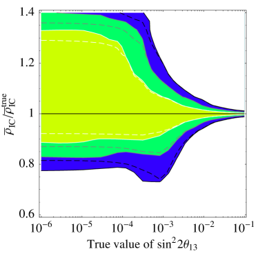
Figure 3: (Color online) The measurement of $\bar{\rho}_{IC}$ as function of the true value of $\sin^{2}2\theta_{13}$ at the $1\sigma$, $2\sigma$, and $3\sigma$ confidence levels (from light to dark shaded regions). For the baselines, $L=2\cdot R_{E}$ combined with $L=3\,000\,\mathrm{km}$ is used. The dashed curves correspond to fixing the oscillation parameters, i.e., to not taking into account correlations and degeneracies.

	$L=2\cdot R_{E}$		$L=12\,510\,\mathrm{km}$
	% error on $\bar{\rho}_{IC}$		% error on $\bar{\rho}_{C}$
$\sin^{2}2\theta_{13}$	$1\sigma$	$3\sigma$	$1\sigma$	$3\sigma$
Combination with $\boldsymbol{L=3\,000\,\mathrm{km}}$:
$0.1$	$-0.5$/$+0.5$	$-1.4$/$+1.4$	$-0.2$/$+0.2$	$-0.6$/$+0.6$
$0.01$	$-1.8$/$+1.7$	$-5.5$/$+5.0$	$-0.6$/$+0.6$	$-1.8$/$+1.7$
$0.001$	$-8.3$/$+6.9$	${-27}$/${+21}$	${-1.8}$/${+2.2}$	${-4.9}$/${+7.0}$
Core crossing baseline alone:
$0.1$	${-0.5}$/${+0.5}$	${-1.4}$/${+1.4}$	${-0.3}$/${+0.2}$	${-0.8}$/${+0.6}$
$0.01$	${-2.1}$/${+5.8}$	${-7.2}$/${+9.2}$	${-0.9}$/${+0.9}$	${-2.4}$/${+2.7}$
$0.001$	${-9.9}$/${+19}$	${-40}$/${+35}$	${-2.3}$/${+2.5}$	${-14}$/${+10}$

Table 1: Per cent errors ($1\sigma$ and $3\sigma$) on $\bar{\rho}_{IC}$ for an inner core crossing baseline and $\bar{\rho}_{C}$ for an inner core touching baseline as labeled in the columns. The upper group of numbers refers to the combination with a baseline $L=3\,000\,\mathrm{km}$, the lower group to the core crossing baseline alone. The numbers are given for different values of $\sin^{2}2\theta_{13}$ and $\delta_{\mathrm{CP}}=0$.

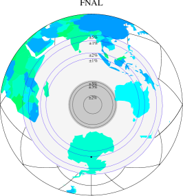
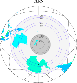
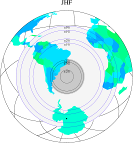
Figure 4: (Color online) Precision of the measurement of $\bar{\rho}^{L}_{C}$ (light gray shaded outer core crossing regions) or $\bar{\rho}^{L}_{IC}$ (dark gray shaded inner core crossing regions) as function of the actual position of the detector for the three laboratories in Fig. 1 as neutrino sources (from west to east). The $1\sigma$ errors are given within the rings as they are labeled. For all setups, the combination with $L=3\,000\,\mathrm{km}$, as well as $\sin^{2}2\theta_{13}=0.01$ are assumed.

In principle, it is enough to have one baseline to measure the average density of the Earth’s core. However, if a neutrino factory is built, it’s main purpose will be the determination of $\delta_{\mathrm{CP}}$ and other sub-leading effects, which means that (for a muon energy of $50\,\mathrm{GeV}$) $L=3\,000\,\mathrm{km}$ is a typical baseline for that purpose (cf., Fig. 1 for potential detector sites). Therefore, we show in Fig. 3 the precision of the measurement of $\bar{\rho}_{IC}$ with $L=2\cdot R_{E}$ as function of the critical parameter $\sin^{2}2\theta_{13}$ in combination with $L=3\,000\,\mathrm{km}$ to reduce the errors of the oscillation parameters. Note that we have chosen the longest possible core-crossing baseline, which is a rather optimistic assumption at first. Fig. 3 demonstrates that $\sin^{2}2\theta_{13}\gtrsim 10^{-3}$ is a prerequisite to obtain high precisions, which also applies to the measurement of $\bar{\rho}_{C}$ (not shown). By comparison of the shaded contours (includes correlations) and the dashed curves (no correlations), it also demonstrates that the combination with $L=3\,000\,\mathrm{km}$ is very close to the optimal (correlation-free) performance. In Tab. 1, the per cent errors are listed for different selected values of $\sin^{2}2\theta_{13}$, where also the values for the core crossing baseline alone and for the measurement of $\bar{\rho}_{C}$ for an inner core touching baseline are shown. From Fig. 3 and Tab. 1 one can easily see that each core crossing baseline alone is almost correlation-free for large values of $\sin^{2}2\theta_{13}$, whereas for small values of $\sin^{2}2\theta_{13}$ the $L=3\,000\,\mathrm{km}$ baseline provides valuable additional information to reduce correlations. The reason for this is that the correlation with $\delta_{\mathrm{CP}}$ is rather unimportant for large values of $\sin^{2}2\theta_{13}$ at these very long baselines, where the contribution from the solar oscillations becomes MSW effect suppressed (see, e.g., LABEL:~Huber:2003ak ). From Tab. 1, we can finally read off a $1\sigma$ error of less than one per cent for $\rho_{IC}$ under optimal conditions, i.e., for large $\sin^{2}2\theta_{13}$ and long enough baselines.

Let us now restrict these optimal assumptions somewhat. As it is obvious from Fig. 1, there may not always be potential detector locations especially for inner core crossing baselines. Therefore, we show in Fig. 4 the precision of the measurement for a somewhat smaller value of $\sin^{2}2\theta_{13}=0.01$ as function of the actual detector location for the laboratories as given in the plot labels. In this case, the optimal precision for the inner core crossing baselines of about $2\%$ can not be reached because there is nothing besides water on the opposite sides of the main laboratories. However, a precision of $3\%$ is easily reachable, since, because of the spherical geometry, baselines through the inner core travel long distances within the inner core for a large region of the inner core shadow region projected onto the Earth’s surface. The same, in principle, applies to the outer core crossing baselines.

In summary, a precision determination of the Earth’s absolute inner or outer core density at the percent level seems to be feasible with a neutrino factory baseline for large enough $\sin^{2}2\theta_{13}\gtrsim 10^{-2}$, even if one takes into account the knowledge on the neutrino oscillation parameters. Since a neutrino factory muon decay ring naturally spans two baselines, such a core crossing baseline could be an additional (or subsequent) payoff of a neutrino factory in addition to its main purpose to measure the neutrino oscillation parameters precicely. The major challenge of such an approach would be building am appropriate decay ring with a vertical decay tunnel. From the geographical point of view, given some of the current potential candidates for a neutrino factory, there are many potential detector locations on the southern hemisphere where sufficient precisions could be obtained. From the neutrino physics point of view, other applications of such a very long baseline would be the degeneracy-free measurement of $\sin^{2}2\theta_{13}$ or the verification of the MSW effect Huber:2003ak .

In comparison to seismic wave geophysics, neutrinos are sensitive to the absolute electron density in matter, which means that the relationship to the absolute matter density is much cleaner from model-dependent assumptions. This measurement could therefore help to test the equation of state for seismic waves. The obtainable relative precision at the percent level is competitive to the relative precisions of the density jumps given by seismic wave geophysics. For example, at the inner core boundary, $\Delta\rho\simeq 0.82\pm 0.18\,\mathrm{g}\,\mathrm{cm}^{-3}$ Masters . Of course, the neutrino factory approach alone is unlikely to give a three-dimensional model of the Earth, but its strength to measure the baseline averaged density as opposed to the volume averaged density makes it a good candidate for direct matter density tests of especially the innermost parts of the Earth.

I would like to thank Peter Goldreich and Jeroen Tromp for useful information and discussions, and Pomita Ghoshal for pointing out an error. This work has been supported by the W. M. Keck foundation.

References

- (1) S. Geer, Phys. Rev. D57, 6989 (1998); M. Apollonio et al. eprint hep-ph/0210192; C. Albright et al. eprint physics/0411123.
- (2) L. Wolfenstein, Phys. Rev. D17, 2369 (1978); S. P. Mikheev and A. Y. Smirnov, Sov. J. Nucl. Phys. 42, 913 (1985).
- (3) V. K. Ermilova, V. A. Tsarev, and V. A. Chechin, Bull. Lebedev Phys. Inst. NO.3, 51 (1988); T. Ohlsson and W. Winter, Europhys. Lett. 60, 34 (2002); A. N. Ioannisian and A. Y. Smirnov eprint hep-ph/0201012; A. N. Ioannisian and A. Y. Smirnov, Phys. Rev. Lett. 93, 241801 (2004); A. N. Ioannisian et al. eprint hep-ph/0407138.
- (4) T. Ohlsson and W. Winter, Phys. Lett. B512, 357 (2001).
- (5) M. Lindner et al., Astropart. Phys. 19, 755 (2003).
- (6) M. Apollonio et al. (CHOOZ), Phys. Lett. B466, 415 (1999).
- (7) P. Huber et al., Phys. Rev. D70, 073014 (2004).
- (8) V. Dehant et al. (editors) Earth’s Core: Dynamics, Structure, Rotation (AGU Geodynamic Series, 2003).
- (9) T. Ohlsson and H. Snellman, Eur. Phys. J. C20, 507 (2001).
- (10) A. M. Dziewonski and D. L. Anderson, Phys. Earth Planet Int. 25, 297 (1981).
- (11) P. Huber, M. Lindner, and W. Winter, Nucl. Phys. B645, 3 (2002).
- (12) P. Huber, M. Lindner, and W. Winter, Comp. Phys. Comm. (to be published), eprint hep-ph/0407333, URL http://www.ph.tum.de/~globes.
- (13) G. L. Fogli et al., Phys. Rev. D67, 093006 (2003); J. N. Bahcall, M. C. Gonzalez-Garcia, and C. Pena-Garay, JHEP 08, 016 (2004); A. Bandyopadhyay et al. eprint hep-ph/0406328; M. Maltoni et al., New J. Phys. 6, 122 (2004).
- (14) M. C. Gonzalez-Garcia and C. Pea-Garay, Phys. Lett. B527, 199 (2002).
- (15) P. Huber and W. Winter, Phys. Rev. D68, 037301 (2003), W. Winter eprint hep-ph/0411309.
- (16) G. Masters and D. Gubbins, Phys. Earth Planet Int. 140, 159 (2003).