a Evolution at small ${x_{\text{bj}}}$: The Color Glass Condensate

Heribert Weigert

Institut für theoretische Physik, Universität Regensburg, 93040 Regensburg, Germany

When probed at very high energies or small Bjorken ${x_{\text{bj}}}$, QCD degrees of freedom manifest themselves as a medium of dense gluon matter called the Color Glass Condensate. Its key property is the presence of a density induced correlation length or inverse saturation scale $R_{s}=1/Q_{s}$. Energy dependence of observables in this regime is calculable through evolution equations, the JIMWLK equations, and characterized by scaling behavior in terms of $Q_{s}$. These evolution equations share strong parallels with specific counterparts in jet physics. Experimental relevance ranges from lepton proton and lepton nucleus collisions to heavy ion collisions and cross correlates physics at virtually all modern collider experiments.

1 Introduction

1.1 QCD in collider experiments at high energies

With the advent of modern colliders, from the Tevatron and HERA to RHIC and planned facilities like LHC and EIC, the high energy asymptotics of QCD has gained new prominence and importance. Needless to say that these facilities have been built with very different research goals in mind. On the particle physics side one finds most prominently the search for the Higgs particle as the last missing ingredient of the standard model and hope for clear evidence of physics beyond it. Here high energies are needed mainly to exceed particle production thresholds to facilitate the generation of telltale signals with sufficiently large cross section. On the nuclear or heavy ion physics side it is the search for the quark gluon plasma and its properties that requires high energies to create the energy densities and temperatures needed to cross the QCD deconfinement phase transition and create a medium of deconfined quarks and gluons whose exact nature is still hotly under debate.

In all these experiments one is talking about enormous center of mass energies per participant (i.e. nucleon): RHIC operates at center of mass energies of $200$GeV/nucleon, LHC in its heavy ion mode is aiming at $2$TeV/nucleon while the pure particle physics experiments will be conducted via proton proton collisions at $7$TeV. This implies enormous boost factors between $200$ and several thousands that will strongly affect the QCD aspects of these experiments. In such an environment one knows that soft gluon emission is enhanced by logarithms that arise from $dE/E$ factors in the phase space measure.

In QED the analogous process of photon emission can be treated by resummation, which gives rise to Sudakov form factors. (These provide the resolution of the well known infrared “problem” in QED.) For the non-Abelian case the situation is more involved. The (Abelian) Sudakov type of exponentiation or eikonalization is still present, but captures only a part of the effects. In QCD the problem of multiple soft emission is intrinsically nonlinear – gluons carry color charge and thus in contradistinction to photons act as sources for further emission. This provides a growth mechanism for cross sections absent in QED. Complementarily, after a sufficient number of soft emission steps, one has to start to consider recombination effects: further emission into a region that is already populated by a large number of other color charges will be modified by recombination and absorption, a mechanism that will invariably slow down further growth in gluon numbers and lead to saturation. Both these effects are irrelevant in QED (suppressed by an additional factor of $\alpha$) and only relevant in the non-Abelian theory. There they are usually associated with the successes and failures of the Balitsky-Fadin-Kuraev-Lipatov (BFKL-) equation [1, 2, 3, 4, 5], which is the prototype of an evolution equation meant to resum soft gluon emissions at high energies. This equation carefully takes into account the multiple emission aspect and in this sense addresses a specifically non-Abelian issue that is absent in QED, but excludes recombination effects that arise at large gluon densities and thus is no longer valid where these become relevant.

The BFKL equation, if taken literally and used beyond this limit of applicability leads to an untamed, characteristic power-like growth of cross sections with cm energy, for instance in deep inelastic scattering (DIS) as conducted in electron proton collisions at HERA. This in itself would lead to a violation of the unitarity bound on cross sections.

On the other side, at vanishing (or just very small) momentum transfer the BFKL equation is plagued by a diffusion into the infrared: gluons are emitted at smaller and smaller momenta and will eventually reach nonperturbative scales where the assumption of small coupling underlying the derivation of the equation is no longer valid.

Both of these main problems of the BFKL equation can be cured by taking into account nonlinear effects in the gluon generation mechanism at high energies, at least for central collisions, where we expect gluon densities to become large. This is the domain of a highly dense gluonic medium and the topic of this review. The main theoretical tool is an associated evolution (or Wilson type renormalization group) equation that describes the creation and change of the medium with increasing energy, the Jalilian-Marian+Iancu+McLerran+Weigert+Leonidov+Kovner equation [7, 8, 9, 10, 11, 12, 13, 14, 15] [the order of names was chosen by Al Mueller to give rise to the acronym JIMWLK, pronounced “gym walk”]. The quite distinct combination of features, the generation of large gluon densities which can arise only in non-Abelian theories, the time scale differences between soft and hard modes that enter the dynamics and the onset of recombination and saturation effects have led McLerran and Venugopalan to coin the term “Color Glass Condensate” (CGC) which subsequently has been generally adopted as a convenient label for this situation in particular with regards to the HERA (electron proton), RHIC (heavy ion) EIC (lepton nucleus) and LHC (both in proton proton and heavy ion mode) experiments.

It should be kept in mind, however, that the central underlying concept, the nonlinear effects in soft gluon emission feature prominently also in other areas. An example that provides opportunities for fruitful comparison can be found in the study of so called non-local jet observables. This is a class of observables in which soft emission from secondary particles –relatively ”hard” jet constituents other than the original leading partons– plays an important role. Accordingly jet evolution can be described by evolution equations that have a, at first sight surprising, strong structural and conceptual analogy with the JIMWLK equation. For so called global observables, where the origin of secondary gluon radiation can be ascribed to the original leading partons, the equations reduce to liner evolution equations that to a large extent are dominated by Sudakov type physics – to a degree that one can even derive evolution equations without any overt reference to medium effects. In the generic case, however, the medium is the crucial ingredient. This situation will be used throughout this review to highlight the generic nature of concepts and the mechanisms appearing in the generation of a dense gluonic medium at high energy, although phenomenology and applications in both cases are quite different.

Returning to the CGC, one has to highlight its generic feature, the creation of a density induced correlation length $R_{s}=1/Q_{s}$. The associated momentum scale $Q_{s}$ is called the saturation scale. They simply characterize the onset of the saturation effects induced by the medium. Beyond $1/Q_{s}$ color charges start to screen each other and since the underlying gluon densities grow with energy, $Q_{s}$ will, by necessity, follow this trend. $Q_{s}$ is the characteristic scale of the medium and responsible for all the “good” features that go beyond the physics of the BFKL equation: Below $Q_{s}$ the growth of the gluon density and thus of certain cross sections is checked on the one hand, and on the other hand the infrared problems are cured: a shrinking correlation length $R_{s}$ prevents the appearance of non-perturbative modes near and below the QCD scale as long as the dense medium is present, in particular for central collisions. Generically, one would expect $Q_{s}$, as the characteristic scale of the medium, also to be the relevant scale for the coupling constant in this situation. This holds true, although it has turned out that the issue is a bit more subtle than initially expected.

As the list of experiments given at the outset already indicates, the situation is quite generic. Given the high energy involved in all these experiments, it is quite obvious that soft gluon emission and thus JIMWLK like evolution should affect all of them, be it a relatively simple experiment such as deep inelastic lepton proton (henceforth referred to by $ep$ or $\gamma^{*}p$, as done at HERA) or lepton nucleus scattering ($eA$ or $\gamma^{*}A$ as planned with the EIC experiment) or proton proton ($pp$), proton nucleus ($pA$) or nucleus nucleus ($AA^{\prime}$) experiments. [$A$ refers to the atomic number of the nucleus involved.] In all of them one expects CGC physics and thus the presence of an energy dependent saturation scale $Q_{s}$ to affect particle production rates and cross sections. This should allow to cross correlate many of these experiments in this respect and gain a clear understanding of the relevance of the CGC in high energy experiments. It should be noted, however, that the tools are most developed for the simple case of deep inelastic scattering of leptons on protons and nuclei. This example then will also be my starting point to introduce the physical ideas –with a minimal amount of formulae– in the following section.

1.2 The CGC in DIS: high energies, gluon densities and the saturation scale

To acquaint the reader with the main features of the CGC, it is perhaps best to refer to the example in which the physics ingredients are best understood and the technical tools that were developed to incorporate them are most directly applicable, deep inelastic scattering of leptons on (preferably large) nuclei. I will attempt to keep the technical details in this section to a minimum. All of the relevant physics ideas collected here will have their theoretical foundations reviewed in later sections.

To start with, consider a collision of a virtual photon that imparts a (large) spacelike momentum $q$ ($Q^{2}:=-q^{2}$ is large) on a nucleus of momentum $p$ as shown in Fig.2. Being spacelike, $Q^{2}$ sets the transverse resolution scale in the problem. At large energies the only other relevant invariant is Bjorken-$x$ (or ${x_{\text{bj}}}$), defined as ${x_{\text{bj}}}:=\frac{Q^{2}}{2p.q}$ as in Fig. 2. ${x_{\text{bj}}}$ has the interpretation of a (total) momentum fraction carried by a struck parton. At small ${x_{\text{bj}}}$ this has the interpretation of a light cone momentum fraction $k^{+}={x_{\text{bj}}}p^{+}$ where $k$ is the momentum of the probed constituent and $p$ the target momentum. ${x_{\text{bj}}}$ directly corresponds to the large boost factor separating (photon) projectile and target (nucleus) via $\frac{1}{{x_{\text{bj}}}}=e^{Y}$ as shown in Fig.2.

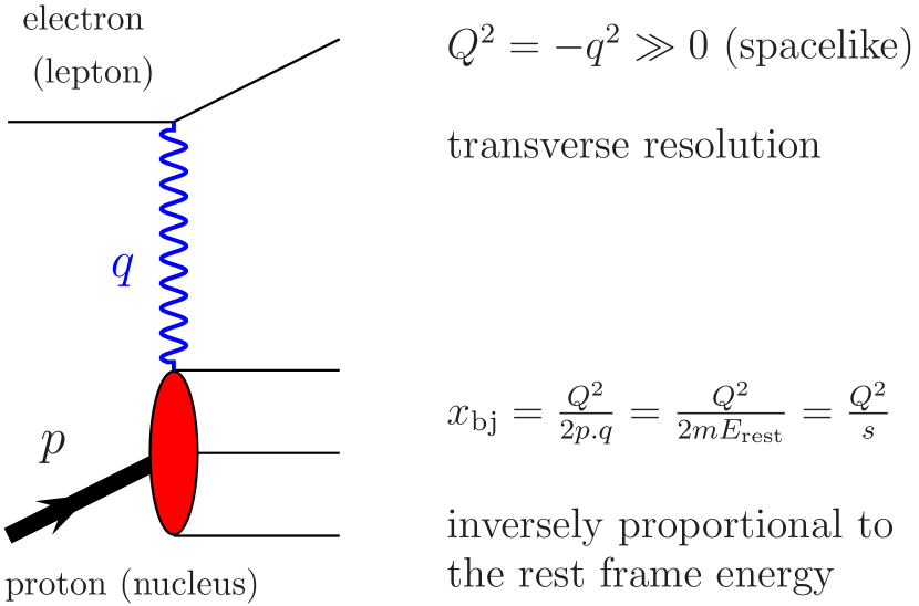
Figure 1: Kinematics in DIS of leptons off protons or nuclei

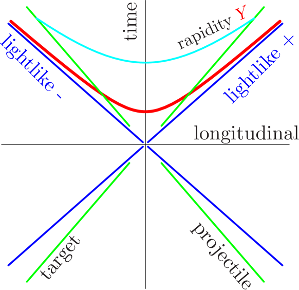
Figure 2: Kinematic variables in a Minkowski diagram. Projectile and target are separated by a large boost factor $\frac{1}{{x_{\text{bj}}}}=e^{Y}$. $x^{\pm}:=\frac{1}{\sqrt{2}}(x^{0}\pm x^{3})$ are the lightlike directions in the $x^{0}$-$x^{3}$ plane often referred to as “$+$” and “$-$” directions.

At high transverse resolutions the situation is simplest. Many quantities, amongst them the total cross section, can be addressed in the framework of an expansion in inverse powers of the transverse resolution $Q^{2}$. This is known as twist expansion and Operator Product Expansion (OPE). Technicalities aside, this expansion has the character of a density expansion: at high resolution a nucleon in the target (which may be a proton in the simplest case) appears to be a dilute system of quarks and gluons. In such a dilute system and in lowest order of the expansion it is sufficient to express the cross section entirely in terms of two point functions, the quark and gluon distributions. Only higher orders of the expansion would involve particle correlations – which are naturally suppressed when densities a small. Nevertheless, even the individual terms in this “density expansion” receive quantum corrections which are important. At large $Q^{2}$ the dominant ones carry factors of $(\alpha_{s}\ln Q^{2})^{n}$ where a large logarithm ($\ln Q^{2}$) compensates for the smallness of the coupling. These contributions need to be resummed to all orders to understand the $Q^{2}$ dependence of quark and gluon distributions at high resolutions. This can be done diagrammatically –known under the keyword ’resummation of ladder diagrams’– or by deriving a renormalization group equation, a differential equation for the distribution functions with respect to $\ln Q^{2}$, the Dokshitzer-Gribov-Altarelli-Parisi (DGLAP) equations. By solving these equations one resums the logarithmically enhanced corrections. In fact, the differential equations are the only information that can be extracted perturbatively: their initial conditions, the quark and gluon distributions at some resolution $Q_{0}$ do contain nonperturbative information about the target. As a consequence one needs experimental measurements over a range of $Q^{2}$ to extract the gluon distributions at $Q_{0}$ by a fit consistent with further evolution. One gains quark and gluon distributions that can be used also in other experiments on the proton. A quite striking result of this procedure is a strong growth of the gluon distributions at small ${x_{\text{bj}}}$ as sketched qualitatively in Fig. 3.

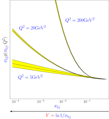
Figure 3: Qualitative growth of gluon distributions as from typical DGLAP fits of DIS at HERA ($eA$) for different $Q^{2}$.

This rise is driven by soft gluon radiation, (sea) quark distributions simply follow their rise.

This procedure is self consistent and perturbatively under control as long as one stays within the large $Q^{2}$ region. Starting from a large enough $Q^{2}_{0}$ and going to larger values, one finds that the objects one counts with the quark and gluon distributions increase in number but they stay dilute: as pointlike excitations their apparent sizes follow the transverse resolution scale $1/Q$. At small ${x_{\text{bj}}}$, however, the growth of the gluon distribution is particularly pronounced – a clear sign that corrections of the form $(\alpha_{s}\ln(1/{x_{\text{bj}}}))^{n}$) start to become important. Any attempt to track the ${x_{\text{bj}}}$-dependence of the cross sections by summing these is immediately faced with an additional complication: moving towards small ${x_{\text{bj}}}$ at fixed $Q^{2}$ increases the number of gluons of apparent size $1/Q$, so that the objects resolved will necessarily start to overlap. This is depicted in Fig. 4.

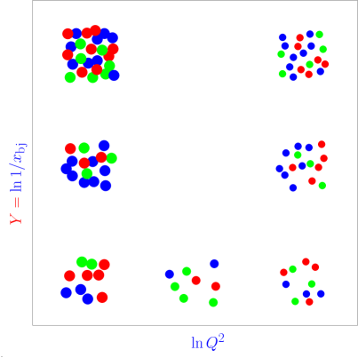
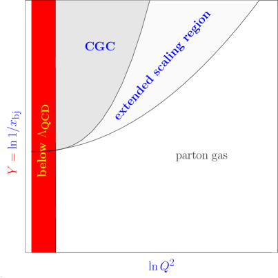
Figure 4: Left: Partons in the $Y,\ln Q^{2}$ plane represented as dots of size $1/Q^{2}$. Numbers grow both with $Q^{2}$ and $\ln(1/{x_{\text{bj}}})$. Going to sufficiently small ${x_{\text{bj}}}$ at fixed $Q^{2}$ partons start to overlap. Right: corresponding regions of phase space with qualitatively different behavior. The lower boudary of the CGC region is determined by $Q_{s}({x_{\text{bj}}})$. The extendeded scaling region will be explaind in Sec. 3.7.

At this point one has long since left the region in which a treatment at leading order in a $1/Q^{2}$ expansion (OPE at leading twist) and the concept of such an expansion itself is meaningful. Instead of single particle properties like distribution functions one needs to take into account all (higher twist) effects that are related to the high density situation in which the gluons in the target overlap. At small ${x_{\text{bj}}}$ one is thus faced with a situation in which one clearly needs to go beyond the standard tools of perturbative QCD usually based on a twist expansion.

There are different ways to isolate the leading contributions to the cross section at small ${x_{\text{bj}}}$ in a background of many or dense gluons and the history of the field is long [16, 17, 18, 19, 20, 21, 22, 23, 24, 25, 26, 27, 7, 8, 9, 10, 28, 11, 29, 30, 31, 12, 13, 14, 15]. I will use a physically quite intuitive picture first utilized in the McLerran-Venugopalan model which was originally given in the infinite momentum frame of the nuclear target. Knowing already that the interaction will be dominated by gluonic configurations, one tries to isolate the boost enhanced ones among them. Looking at the gluon field strength of the target for that purpose, one finds that only the $F^{+i}$ components are boost enhanced, all others can be neglected. At the same time one finds a strong Lorentz contraction in $x^{-}$ direction, and a time dilation, correspondingly, in $x^{+}$ direction. With such a field strength tensor, one is left with only one important degree of freedom, which, by choice of gauge, can be taken to be the + component of a gauge field. Taking into account time dilation and Lorentz contraction, the gauge field can then be written as

$$\begin{split}A=&b+\delta A\qquad\mbox{with}\qquad b^{i,-}=0,\quad b^{+}=\beta(\bm{x})\delta(x^{-})\ .\end{split}$$ (1)

where $\beta$ is an unspecified function of the transverse components $\bm{x}:=(x^{1},x^{2})$ of the four vector $x$. This exhibits a leading contribution $b^{+}$ which is $x^{+}$ independent and Lorentz contracted to a $\delta$-function in $x^{-}$. The $\delta A$ symbolizes possible corrections that are kinematically suppressed. They will start to play a role as quantum corrections in the derivation of evolution equations. The boost and Lorentz contraction arguments for the leading contribution $b$ are ${x_{\text{bj}}}$ dependent. In the interpretation of ${x_{\text{bj}}}$ as a lightcone momentum fraction it determines a resolution in $x^{-}$: the $\delta(x^{-})$ in (1) is “localized” only with the resolution available with a probe providing the corresponding momentum fraction. A similar cautionary remark applies to the $x^{+}$ independence.

Note that mathematically one can always trade a component of a gauge field for a path-ordered exponential along the direction that picks up this component:

$$b^{+}=i(\partial^{+}U)U^{\dagger}\hskip 28.45274ptU_{\bm{x}}={\sf P}\exp\Big{\{}-i\int\!\!dz^{-}b^{+}(z^{-},{\bm{x}},0)\Big{\}}\ .$$ (2)

If multiple eikonal interactions are relevant as the high energy nature of the process would suggest, one expects these path ordered exponentials to be the natural degrees of freedom, since this is what they encode: Diagrammatically

$$U_{\bm{x}}=\sum\limits_{\text{gluons}}\parbox{113.81102pt}{\includegraphics[width=113.81102pt]{gluon-eik}}\ ,$$ (3)

where the path ordered integrals along $z^{-}$ are represented by the fermion line. Ignoring the small fluctuations $\delta A$ for a moment, one has a picture in which the $\gamma^{*}$ nucleus cross section arises from a diagram in which the photon splits into a $q\bar{q}$ pair which then interacts with the background field. Due to the $\delta$ like support of $b^{+}$ the $q\bar{q}$ are not deflected in the transverse direction during that interaction. This just reflects the largeness of the longitudinal momentum component of these partons at small ${x_{\text{bj}}}$. This is shown in Fig. 5. To be sure, the physics content is not frame dependent although it is encoded differently in, say the rest frame of the target. There, one encounters neither Lorentz contraction nor time dilation. However the scale relations are preserved: the photon splits into a $q\bar{q}$ pair far outside the target and its $p^{-}$ is so large that typical $x^{+}$ variations of the target are negligible during the interaction. As a consequence the probe is not deflected in the transverse direction, picking up any multiple interactions with (gluonic) scattering centers as it punches though the target. This is shown in Fig. 5.

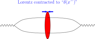
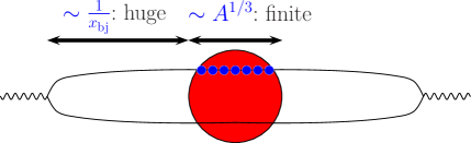
Figure 5: $q\bar{q}$ pairs interacting with a nuclear target at small ${x_{\text{bj}}}$. (a) shows the situation in the targets infinite momentum frame with fully Lorentz-contracted target fields, (b) shows the situation in the target rest frame in which the $\gamma^{*}q\bar{q}$ vertex is far outside the target at a distance proportional to the relative boost factor $1/{x_{\text{bj}}}=e^{Y}$.

That multiple interactions are of relevance immediately becomes obvious, once one tries to calculate such diagrams with a background field method. To this end one evaluates the diagram shown in Fig. 5 in the background of a field of the type shown in Eq. (1) ignoring the small fluctuations. Such a calculation will prove somewhat involved irrespective of the method chosen –one of them will be sketched in Sec. 2– but the resulting expression

$$\sigma_{\mathrm{DIS}}({x_{\text{bj}}},Q^{2})=\text{\cal Im}\ \begin{minipage}[c]{85.35826pt} \includegraphics[height=22.76228pt]{dipole} \end{minipage}=\int\!\!d^{2}r\,|\psi^{2}|(r^{2}Q^{2})\hskip 2.84544pt\int d^{2}b\ \langle\frac{{\rm tr}(1-U_{\bm{x}}U^{\dagger}_{\bm{y}})}{N_{c}}\rangle$$ (4)

has a clearcut interpretation. Beginning with notation, $\bm{r}=\bm{x}-\bm{y}$ corresponds to the transverse size of the $q\bar{q}$ dipole and $\bm{b}=(\bm{x}+\bm{y})/2$ to its impact parameter relative to the target. This result shows a clear separation into a wave function part (the factor $|\psi^{2}|(r^{2}Q^{2})$) and the dipole cross section part

$$\sigma_{\text{dipole}}(Y=\ln(1/{x_{\text{bj}}}),r^{2}):=\int d^{2}b\ \langle\frac{{\rm tr}(1-U_{\bm{x}}U^{\dagger}_{\bm{y}})}{N_{c}}\rangle_{Y=\ln(1/{x_{\text{bj}}})}\ .$$ (5)

The former has the interpretation as the absolute value squared of the $q\bar{q}$ part of the photon wave function, contains the $\gamma^{*}q\bar{q}$ vertices and can, alternatively to the background field method, be calculated entirely within QED. The wave functions themselves turn out to be Bessel functions $K_{0,1}$ depending on the polarization of the virtual photon. This factor carries all of the direct $Q^{2}$-dependence of the cross section.

The dipole cross section part embodies all the interaction with the background gluon fields in terms of the path ordered exponentials. In particular, in the absence of a gluon field representing the interaction with the target, both $U$ factors reduce to unit matrices and the cross section vanishes. The averaging procedure $\langle\ldots\rangle_{Y}$ contains all the information about the QCD action and the target wave functions that are relevant at small ${x_{\text{bj}}}$.

Even without exploring any of these in detail, there is one feature about this interaction which is very characteristic for DIS at small ${x_{\text{bj}}}$ which is already visible in the above expression: although momentum is exchanged between projectile and target, there is no net color exchange: the $q\bar{q}$ pair enters and leaves the interaction region as a color singlet. The same applies to other intrinsic quantum numbers such as spin. In a diction dating back to pre-QCD times this is often referred to as “pomeron exchange,” although it is now acknowledged that the underlying theory of the interaction does not exhibit a particle cut that would allow an interpretation in terms of a simple particle exchange.

It is fairly clear from the above discussion, that the isolation of the leading $b^{+}$ contribution which defines this average is a resolution dependent idea: as one lowers ${x_{\text{bj}}}$, additional modes –up to now contained in $\delta A$ of Eq. (1)– will take on the features of $b^{+}$. They will Lorentz contract and their $x^{+}$-dependence will freeze. Accordingly the averaging procedure will have to change. If one writes the average as

$$\langle\ldots\rangle_{Y}=\int D[b^{+}]\ldots W_{Y}[b^{+}]\hskip 14.22636pt\text{or, equivalently}\hskip 14.22636pt\langle\ldots\rangle_{Y}=\int\hat{D}[U]\ldots\hat{Z}_{Y}[U]\ ,$$ (6)

the weights $W_{Y}[b^{+}]$ or $\hat{Z}_{Y}[U]$ will, by necessity, be $Y=\ln(1/{x_{\text{bj}}})$ dependent.

Besides the perspective adopted above, there are equivalent ways to understand and derive the ${x_{\text{bj}}}$ dependence of such cross sections in which the path ordered exponentials do not appear in closed form in the first calculational step but instead are built up perturbatively. Among those is the most straightforward procedure in which one allows the incoming $q\bar{q}$ (into which the incoming $\gamma^{*}$ splits initially) to branch off additional gluons before it hits the target. Looking at the corresponding amplitudes this would amount to consider perturbative corrections to the $\gamma^{*}\to q\bar{q}$ amplitude contained in Fig. 5 of the form

$$\begin{minipage}[c]{42.67912pt} \begin{center} \includegraphics[height=56.9055pt]{bareqqb} \end{center} \end{minipage}+\begin{minipage}[c]{71.13188pt} \begin{center} \includegraphics[height=56.9055pt]{qqb-gu} \end{center} \end{minipage}+\begin{minipage}[c]{71.13188pt} \begin{center} \includegraphics[height=56.9055pt]{qqb-gd} \end{center} \end{minipage}+\begin{minipage}[c]{71.13188pt} \begin{center} \includegraphics[height=56.9055pt]{qqb-g2u} \end{center} \end{minipage}+\begin{minipage}[c]{71.13188pt} \begin{center} \includegraphics[height=56.9055pt]{qqbggsplitu} \end{center} \end{minipage}+\ldots\ \ .$$ (7)

All but the last of these diagrams would be present already in QED. It is this last type of contribution that is responsible for the strong growth and the saturation features of the CGC. That all these methods lead to the same result will be thoroughly explained in the main text.

Fig. 6 highlights another feature of the dominant contributions: as the distance between the $\gamma^{*}\to q\bar{q}$ vertex and the target grows with increasing energy like the corresponding boost factor, the probability of multiple gluon emission grows accordingly. This leads to the iterative scheme indicated in Fig. 6 (with only part of the above diagrams displayed for brevity).

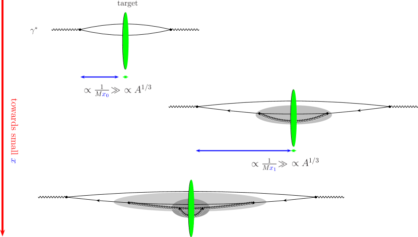
Figure 6: RG corrections to the average over background field configurations. The shaded areas contain the contributions subsumed into the averaging procedure at successive values of $Y=\ln(1/{x_{\text{bj}}})$.

Note that the leading contributions come, as usual, from ordered emission, so that the lines depicted there all have large momentum components in the photon direction. They themselves will then interact with the target in a similar way as the original $q\bar{q}$ component: These punch straight through the target at fixed transverse locations $\bm{x}$ and $\bm{y}$, giving rise to the $U_{\bm{x}}U^{\dagger}_{\bm{y}}$ in the expression for the cross section in Eq. (4). The additional gluons shown in Eq. (7) and Fig. 6 leave behind new gluonic Wilson lines $\tilde{U}$ (the tilde indicating that they are in the adjoint representation) at new locations $\bm{z}_{i}$. It is clear from gauge invariance that the second diagram in Fig. 6 will involve the operator $\tilde{U}_{\bm{z}}^{ab}\ 2{\rm tr}(t^{a}U_{\bm{x}}t^{b}U^{\dagger}_{\bm{y}})$ where $\tilde{U}_{\bm{z}}^{ab}$ represents the added gluon. From this perspective one would expect that calculating additional corrections would lead to an infinite hierarchy of coupled equations for more and more complicated correlators of Wilson lines. This indeed is the perspective taken by Balitsky in his derivation of this hierarchy of evolution equations [26], the Balitsky hierarchy. The perspective taken above is different in the sense that these same diagrams have been interpreted to contribute a change in the averaging procedure that describes the dipole cross section of Eq. (5). The $q\bar{q}$ dipole at smaller ${x_{\text{bj}}}$ is taken to interact with additional gluons and thus the cross section and averaging procedure changes. In Fig. 6 this redefinition process is indicated by the shaded areas that include the target, and subsequently the target and all the gluons softer than the initial $q\bar{q}$ pair. Both approaches are indeed equivalent as will become apparent from the mathematical treatment.

As these descriptions indicate, it is possible to calculate the change of the weights in Eq. (6) with $Y$ to a certain perturbative accuracy – at the moment complete calculations of these evolution equations based on independent techniques exist at leading log accuracy, i.e. to accuracy $\alpha_{s}\ln(1/{x_{\text{bj}}})$– while $\hat{Z}_{Y}[U]$ at a given $Y_{0}$ remains incalculable without nonperturbative input. This is again the situation one has to face in any Renormalization Group (RG) setting in which the initial condition for evolution remains outside the scope of the calculation and must be determined from experiment.

The renormalization group character of the calculation can be made explicit by assuming one knew, say $\hat{Z}_{Y}[U]$ at an initial $Y_{0}$. This defines the ensemble of initial background fields $b^{+}$ and one may then integrate over the fluctuations $\delta A$ around $b^{+}$ between the old and new cutoffs $Y_{0}$ and $Y_{1}$. Taking the limit $\delta Y=Y_{1}-Y_{0}\to 0$ one then gets a renormalization group equation for $\hat{Z}_{Y}[U]$.

Because one integrates over $\delta A$ in the background of arbitrary $b$ of the form (1), the equation treats the background field exactly to all orders and captures all nonlinear effects also in its interaction with the target. The resulting RG equation is a functional equation for $\hat{Z}_{Y}[U]$ that is nonlinear in $U$. It sums corrections to the leading diagram shown in Eq. (4) in which additional gluons are radiated off the initial $q\bar{q}$ pair as shown schematically in Fig. 6. All multiple eikonal scatterings inside the target (the shaded areas) are accounted for.

The result of this procedure is the JIMWLK equation alluded to above. This equation and its limiting cases will be discussed in detail in Sec.3.

Let me close here with a few phenomenological expectations for the key ingredient of the present phenomenological discussion, the dipole cross section. Clearly, one expects the underlying expectation value of the dipole operator,

$$N_{Y\ \bm{xy}}:=\langle\frac{{\rm tr}(1-U_{\bm{x}}U^{\dagger}_{\bm{y}})}{N_{c}}\rangle_{Y=\ln(1/{x_{\text{bj}}})}\ ,$$ (8)

to vanish outside the target, so that the impact parameter integral essentially samples the transverse target size and thus scales roughly with $A^{2/3}$. For central collisions, i.e. deep inside the target, $N_{Y,\bm{xy}}$ is expected to interpolate between zero at small $\bm{r}=\bm{x}-\bm{y}$ and one at large $\bm{r}$. Note that $N_{Y,\bm{xy}}$ is necessarily limited to lie inside these boundaries as an immediate consequence of the resummation of the gluon fields into eikonal factors $U^{(\dagger)}$. Saturation of these limits at small and large distances is the idea of color transparency for small dipoles supplemented with saturation for large dipoles and is sketched schematically in Fig.7.

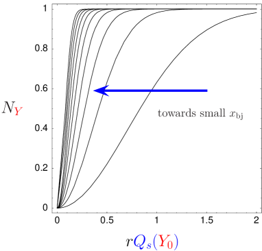
Figure 7: Generic evolution trend for a one scale dipole correlator $N_{\bm{xy}}$ plotted against $|\bm{x}-\bm{y}|$ as $x\to 0$: the curves move towards the left as $Y=\ln(1/{x_{\text{bj}}})$ increases, the asymptotic form being a step function at the origin.

Focusing on the rightmost curve in Fig.7 which corresponds to $Y_{0}$ one has a single scale, $Q_{s}(Y_{0})=1/R_{s}(Y_{0})$, that characterizes the transition between transparent and saturated, hence its name, saturation scale. Looking back at the definition of $N_{Y\ \bm{xy}}$ in terms of the relevant fields $U^{(\dagger)}$, it is clear that the region where it differs from unity is simply the region where the fields are correlated: $R_{s}=1/Q_{s}$ has the interpretation of a correlation length. From this it is apparent that evolution towards smaller ${x_{\text{bj}}}$ at fixed $Q^{2}$ (along vertical lines in Fig.4), which will add more gluons, will necessarily lead to shorter correlation length and thus larger saturation scales: The curve will move toward the left as indicated, with smaller and smaller $R_{s}(Y)$ characterizing the changeover between the two regimes. Since small ${x_{\text{bj}}}$ evolution equations respect the generic saturation features shown in Fig. 7, $Q_{s}$ is also the scale that characterizes the onset of color recombination effects that slow down and eventually stop the growth of the dipole cross section for large dipole sizes.

From here one can immediately understand that going from small to large hadronic targets (i.e. by increasing the target’s atomic number $A$) one also increases the apparent gluon density in this kinematic domain: The starting point again is that the energy is assumed to be high enough that the projectile would punch straight through the target so that multiple scattering contributions sum into the eikonal factors entering $N_{Y\ \bm{xy}}$. In large nuclei, one scatters off gluons from many independent nucleons along the $q\bar{q}$ trajectory as sketched in Fig. 8.

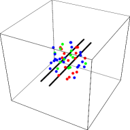
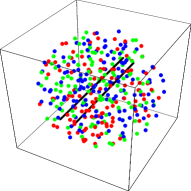
Figure 8: The origin of growth of $Q_{s}$ with $A$ in dilute targets with decorrelated scattering centers in longitudinal direction for a small and a large nuclear target. The lines indicate the $q\bar{q}$ pair, the dots the uncorrelated scattering centers.

Following the Lorentz contraction argument from above, the whole depth of the nucleus contributes to the charge density seen at a point in the transverse plane. Since, due to confinement, gluons from different nucleons –encountered at different longitudinal positions– are necessarily decorrelated, this naturally leads to a rescaling of the transverse correlation length $R_{s}^{2}$ by the inverse nuclear radius. Since the nuclear volume scales with the atomic number $A$, this implies scaling of $Q_{s}^{2}$ with $A^{1/3}$:

$$Q_{s}^{A}({Y_{0}})^{2}\sim Q_{s}^{p}({Y_{0}})^{2}\ {A^{1/3}}\ .$$ (9)

This behavior will reappear in a model that was developed to describe qualitative features of saturation effects at small ${x_{\text{bj}}}$, the McLerran-Venugopalan (or MV) model, and explains the interest in studying DIS at small ${x_{\text{bj}}}$ off large hadronic targets. The argument leading to Eq. (9) is simplistic and a more careful treatment will lead to a modification of the $A$ dependence –although an enhancement typically persists. The most obvious source of such modifications are correlations induced by evolution towards smaller ${x_{\text{bj}}}$. This is why the scaling relation is written for some initial (not too small) $Y_{0}$ at which such effects can be expected to be small.

Returning to the ${x_{\text{bj}}}$ dependence sketched in Fig. 7, it is crucial to note that such behavior has far reaching consequences as it leads to perturbative consistence of the RG approach described above. If one takes the $Y$ dependence of $N$ sketched in Fig. 7 as given, any RG equation that leads to this behavior will predict the largest changes at momentum scales of the order of $Q_{s}(Y)$ – this is where the infinitesimal change between neighboring curves and thus the r.h.s. of the corresponding evolution equation peaks. Contributions at momenta below $Q_{s}$ are strongly suppressed. As $Q_{s}$ grows with $Y$, evolution moves away from $\Lambda_{\text{QCD}}$ and thus remains perturbative. This is illustrated in Fig. 9, which shows the curves of Fig. 7 in a 3d plot on the left and the scales active in the evolution equation i.e. $\partial_{Y}N_{Y}$ on the right.

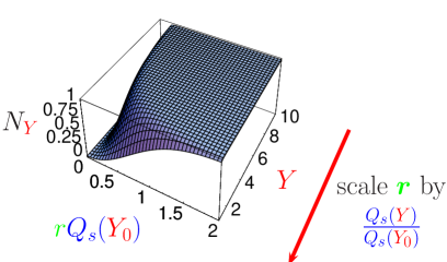
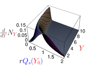
Figure 9: Dipole function (left) and its rapidity derivative (right) for central collisions plotted against dipole size. The latter shows that the change induced by evolution happens at larger and larger momentum scales. This implies IR safety.

Fig. 9 anticipates a further characteristic feature of evolution towards small ${x_{\text{bj}}}$ that, at this point, can not be predicted, but was observed in DIS data by Golec-Biernat and Wüsthoff (G-B+W) [32, 33, 34], namely scaling with $Q_{s}(Y)$, a phenomenon called geometric scaling [34] by Stasto, Golec-Biernat, and Kwiecinski. They have found that for ${x_{\text{bj}}}$ values below $10^{-2}$ all HERA data show beautiful scaling, if in Eq.(5) one assumes the scale in the $\bm{r}$ dependence carries at the same time all the $Y=\ln(1/{x_{\text{bj}}})$-dependence according to

$$N_{Y\ \bm{xy}}=N((\bm{x}-\bm{y})^{2}Q_{s}(Y)^{2})\ .$$ (10)

Such scaling takes all the curves represented in Fig. 9 and maps them onto a single curve as shown in Fig. 10.

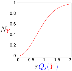
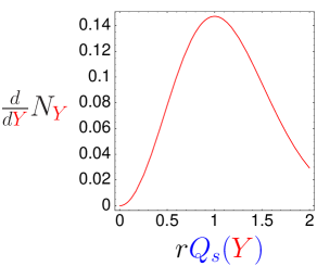
Figure 10: $Q_{s}$ scaled version of Fig.9 assuming that geometric scaling holds.

The same carries through to the DIS cross section via Eq. (4) and leads to the successful fit of the HERA data just alluded to.

There are many more physics ideas associated with the label CGC, such as the existence of an extended scaling region at resolutions $Q$ above $Q_{s}$ indicated already in Fig. 4, which is quite important for the conceptual consistency of the scaling fit to HERA data, the relevance of the CGC to the initial conditions of heavy ion collisions, consequences for particle multiplicities and the Cronin effect, as well as an intimate relationship with other QCD phenomena that involve soft gluon emission such as jet physics. Among the core observations is the fact that the JIMWLK evolution equation intrinsically leads to the scaling behavior discussed in Figs. 9 and 10.

Many phenomenological applications are based on this scaling behavior and I strongly recommend to have a first glance at Sec. 8 to get an idea of the broad range of affected phenomena before delving into the main text. This should provide additional a strong motivation to understand the underlying theoretical tools and evolution equations.

1.3 How to read this review

Having given a brief overview over the core physics ideas in the previous subsection, it is left to the body of the paper to substantiate these claims and flesh out the context from which they arise.

This review contains two interwoven threads of arguments, one of them centered around the derivation of evolution equations that govern soft gluon emission from QCD at small coupling but large gluonic densities, the other aimed at exploring their consequences and interpretation using models and numerical work as well as phenomenological applications. They can of course not be fully separated. Clearly the theoretical grounding is necessary for any application, but also the other direction is vital: for instance the numerical work in [35] has had consequences on the understanding of the necessity of running coupling corrections, not only in a quantitative, but also a conceptual sense. Similarly, the discovery of geometric scaling in HERA data has prompted a look for scaling features in the evolution equations. This in mind, the paper develops both threads in stages. It presents a different perspective on the derivation and interpretation of the underlying evolution equations than other existing reviews [36, 37], not the least by highlighting the parallels with nonlinear effects in jet physics in Sec. 5. I have also been aiming at exposing the close connection between the McLerran Venugopalan model with the BK equation in Sec. 3.5. These formulations have not been shown elsewhere, but are hidden under the surface of many discussions of the Glauber-Mueller type nature of the multiple scattering phenomena omnipresent in small ${x_{\text{bj}}}$ physics. I have attempted to present an up to date description of the role of BFKL physics as the driving force of small ${x_{\text{bj}}}$ evolution and have included results of numerical simulations of the full JIMWLK equations as well as a thorough discussion of running coupling in the BK case.

Sec. 2 is devoted to the first important type of nonlinearity encountered: eikonalization of soft gluon fields into path ordered exponentials often also called eikonal factors or Wilson lines. Sec.2.1 aims at explaining their appearance in cross sections and propagators and Sec.2.2 discusses an immediate consequence, boundedness of the underlying correlators, in terms of the MV model and its generalizations. The link to gluon distributions, density effects and $A$ scaling also appear in this context.

Sec. 3 then gives an overview over the formulation of the JIMWLK equation and the associated physics ideas. It starts off firmly in the formal thread with the full derivation in Sec. 3 – I consider this quite informative, but the reminder can be followed without having read this in a first go. Sec. 3.2 explains the JIMWLK Hamiltonian, its properties and the nature of the equation as a Fokker-Planck equation. Sec. 3.4 formulates the idea of scaling in the context of these evolution equations and Sec. 3.5 discusses the relation of JIMWLK, BK and BFKL (in both forward and nonforward cases) equations from the perspective of $N_{c}$ and density expansions. How the underlying growth pattern is imprinted by BFKL physics is discussed in Sec. 3.6. This gives rise to the idea of a scaling window as emphasized in Sec. 3.7 and already shown in Fig. 4 as the extended scaling region.

Sec. 4 performs a translation of the JIMWLK equation to a Langevin type formalism: Sec.4.1 gives a toy example to illustrate the idea while Sec.4.2 gives the result which is the basis for numerical simulations. Sec.4.3 introduces shower operators which will, in Sec. 5 find an interpretation as operators that generate the soft gluon cloud in the photon wavefunction and counts among the conceptual developments.

Sec. 5 leads up to this interpretation and helps to understand that JIMWLK evolution shows a structure which is generic for soft gluon emission physics. This is illustrated with an example from the context of non-global jet observables for which Sec. 5.1 and 5.2 give evolution equations with clear structural analogies to BK and JIMWLK. Next is a derivation of these equations which may be skipped in a first reading. In this derivation one first constructs the leading part of generic soft n-gluon amplitudes (corresponding to the photon wave functions) in Sec. 5.4. As a second step one utilizes the iterative nature of the construction process to extract a corresponding evolution equation in the next subsections. Sec. 5.7 highlights the two types of nonlinearities encountered in the derivation –eikonalization and nonlinear evolution– and explores $N_{c}$ or correlator factorization once more in the jet situation.

Sec. 5.8 briefly discusses the lessons to be learned for small ${x_{\text{bj}}}$ evolution from the preceding section and provides a first glance at what is to be expected if jets are created inside a dense medium.

Sec. 6 and 7 discuss numerical results from solving JIMWLK and BK evolution equations. Discussed are scaling, 6.1, correlator factorization violations, 6.2, and the problems of fixed coupling simulations in the UV, 6.3. With running coupling UV phase space is under control and allows quantitative studies of $Q_{s}$ and the scaling features, 7.1. This subsection contains the core results on scaling behavior. Sec. 7.2 returns to $A$ scaling already introduced in the MV model and discusses the changes imposed by evolution.

Sec. 8 tries to give a flavor of the phenomenology associated with the previous theoretical results. Highlighted are geometric scaling, initial conditions of heavy ion collisions, consequences for the Cronin effect and a few more.

Experimental efforts in connection with RHIC, LHC and EIC increase the pressure to come up with more observable consequences and better tools to make predictions – a few ideas are mentioned in the conclusions, Sec. 9.

2 Eikonalization at high energies

2.1 Propagators and cross sections

There are two distinct types of nonlinearities present in the formulation of cross sections and their ${x_{\text{bj}}}$ dependence as presented in Sec.1.2, the first is the resummation of the gluon field into path-ordered exponentials $U^{(\dagger)}_{\bm{x}}$ collinear to the projectile, the second is the nonlinearity of the evolution in correlators of this type of field. The first aspect is present already in the Abelian theory, the second appears only in the non-Abelian case but can not be separated from the first. Without the first step, the identification of the relevant variables, all the following steps have no proper foundation and formulae like Eq.(4) remain mysterious. Let me, therefore, start with identifying the variables and a brief derivation of this formula for the DIS cross section.

The starting point is the kinematics. A collision at large energies singles out a longitudinal direction, say $x^{3}$, as the collision axis. In such a frame the large energy is characterized by a big rapidity separation between target and projectile. To judge how a projectile, say the $q\bar{q}$ dipole emerging at lowest order in the photon wave function of Eq. (4), sees the target, it is best to consider the color Field generated by the target. Remembering that light cone components $x^{\pm}:=\frac{1}{\sqrt{2}}(x^{0}\pm x^{3})$ are eigendirections of a boost in $3$ direction ($x^{\pm}\to e^{\pm Y}x^{\pm}$ with $\gamma=e^{Y}=\frac{1}{\sqrt{1-v^{2}/c^{2}}}$) it becomes clear that the components of the field strength tensor are enhanced by a factor $e^{Y}$ in the plus components and suppressed by a factor $e^{-Y}$ in the minus components. At the same time Lorentz contraction “shrinks” the support of the color field to a (near) delta function in $x^{-}$ and time dilatation renders it (nearly) independent on $x^{+}$. The leading components are

$$F^{i+}(x)=\delta(x^{-})\partial^{i}\beta(\bm{x})\ .$$ (11)

On the r.h.s. I have already made use of the gauge freedom to express $F^{i+}$ via a single scalar function which can be associated with the $b^{+}$ of Eq. (1) and (2).

To calculate cross sections like (4), one needs to consider current correlators of the form $\langle J^{\mu}(u)J^{\nu}(v)\rangle$ in the background field representing the target and subtract noninteracting counterpart (to go from an S-matrix to a T-matrix contribution). To lowest order, the cross section (4) then takes the form

$$\sigma_{\mathrm{DIS}}({x_{\text{bj}}},Q^{2})=\text{Im}\ \begin{minipage}[c]{85.35826pt} \includegraphics[height=22.76228pt]{dipole} \end{minipage}=\text{Im}\left\langle\parbox{85.35826pt}{\includegraphics[width=85.35826pt]{dipcross-curr-diag}}-\parbox{85.35826pt}{\includegraphics[width=85.35826pt]{dipcross-curr-diag-free}}\right\rangle$$ (12)

where the interaction with the target is now explicitly trough the fermion propagators in a background field and the average $\langle\ldots\rangle$ is over background fields $b$ as mandated by the interaction with the target. The simplification lies in the fact that the types of field allowed to enter the interaction is restricted to the type in (11). With it one can find results for cross sections and also include perturbative corrections that will modify (12) once quantum fluctuations around $b$ become large.

The latter will be discussed in detail in later sections, here I am interested in the physics aspect of the calculation leading to (4). The core element here is the background field propagator which encodes all the interaction with the target. It is sufficient to study this propagator to understand the origin of the eikonal factors in the dipole cross section as well as the general form of the result. The key physics insight will be that the interaction is solely mediated through an exchange of momentum.

Besides these physics results, gauge invariance is a somewhat delicate issue: While parametric enhancement and Lorentz contraction of components in the Field strength tensor can be argued in a gauge independent manner, the extraction of path-ordered exponentials that lead to formulae like Eq. (4) appears to be gauge dependent: What happens in a gauge in which one forces the “+” component of the gauge field to zero? This will be briefly touched upon towards the end of this section.

To explore the situation, consider the propagator of a scalar field in the background of some gauge field. This quantity has also been used as the core ingredient to the gluon propagator in [13] in the derivation of the final form of the JIMWLK equation. Using first a Schwinger parameter representation and then standard (nonrelativistic) Feynman-pathintegral techniques in which the Schwinger parameter takes the role of “time,” one writes its propagator as

$$\frac{-i}{D^{2}[b]}(x,y)=\int_{0}^{\infty}dse^{-siD^{2}[b]}=\int^{\infty}_{0}ds\int_{y}^{x}[dz]e^{-\int^{s}_{0}d\kappa\frac{(\dot{z}(\kappa))^{2}}{4}}\ {\sf P}\exp\Big{\{}-ig\int_{y}^{x}dz^{\mu}b_{\mu}(z)\Big{\}}$$ (13)

where the path-integral is over trajectories $z$, parametrized by $\kappa$, that connect $x$ (at $\kappa=0$) to $y$ (at $\kappa=s$). The expression at $b=0$ is the free propagator. Based on the kinematical arguments above, the background field is of the form given in (1): $b^{\mu}(z)=g^{\mu}_{\ +}\delta(z^{-})\beta(\bm{z})$. This implies that only the “$-$” component of the trajectories are probed and only a dependence on the transverse coordinates $\bm{z}$ remains. Due to the $\delta(z^{-})$ shape one finds free propagation unless $x$ and $y$ are on different sides of the $z^{-}=0$ hyperplane, in which case a nontrivial contribution from the path-ordered exponential emerges with free propagation before and after. Since the field is concentrated at $z^{-}=0$, one may deform the eikonal factors outside the $z^{-}=0$ hyperplane into straight line eikonals according to

$${\sf P}\exp\Big{\{}-ig\int_{y}^{x}dz^{\mu}b_{\mu}(z)\Big{\}}\to{\sf P}\exp\Big{\{}-ig\int\limits_{y^{-}}^{x^{-}}\!dz^{-}\,b^{+}(0,{\bm{z}},z^{-})\Big{\}}$$ (14)

and one has to distinguish 4 cases depending on which side of $0$ one places $x^{-}$ and $y^{-}$. For $x^{-}>0>y^{-}$ it is possible to extend the path to cover the whole line from, $\bm{z}-\infty n$ to $\bm{z}+\infty n$ ($n$ a lightlike vector in “$-$” direction). This is what has been denoted $U_{\bm{z}}$ throughout:

$$U_{\bm{z}}:={\sf P}\exp\Big{\{}-ig\int\limits_{\bm{z}-\infty n}^{\bm{z}+\infty n}\!dz^{-}\,b^{+}(0,{\bm{z}},z^{-})\Big{\}}\ .$$ (15)

For $x^{-}<0<y^{-}$ one obtains $U^{\dagger}_{\bm{z}}$ and for same side propagation –with $x^{-},y^{-}>0$ or $x^{-},y^{-}<0$– one simply gets the unit matrix and thus the free propagator. Following the lines of [26] one eventually arrives at an explicit expression for the scalar propagator of the form

$$\left[\frac{-i}{D^{2}[b]}\right]_{ab}(x,y)= \int\!\!\frac{dp^{-}}{2p^{-}(2\pi)^{3}}\left[\theta(x^{-}-y^{-})\theta(p^{-})-\theta(y^{-}-x^{-})\theta(-p^{-})\right]\int\!\!{d^{2}{\bm{p}}^{\prime}d^{2}{\bm{q}}^{\prime}}$$

$$\times\left[e^{-ip^{\prime}.x}\int\!\frac{d^{2}{\bm{z}}}{(2\pi)^{2}}\ e^{-i({\bm{p}}^{\prime}-{\bm{q}}^{\prime}){\bm{z}}}\ {\sf P}\exp\Big{\{}-ig\int\limits_{y^{-}}^{x^{-}}\!dz^{-}\,b^{+}(0,{\bm{z}},z^{-})\Big{\}}e^{iq^{\prime}.y}\right]$$ (16)

where some of the components of these momenta are interrelated according to ${p^{\prime}}^{+}-\frac{{\bm{p}}^{2}-{{\bm{p}}^{\prime}}^{2}}{2p^{-}}=\frac{{{\bm{p}}^{\prime}}^{2}}{2p^{-}}$, ${q^{\prime}}^{+}=\frac{{{\bm{q}}^{\prime}}^{2}}{2p^{-}}$ and ${p^{\prime}}^{-}={q^{\prime}}^{-}=p^{-}$. The massive version simply has on-shell “$+$” momenta shifted by $m^{2}/2p^{-}$. An alternative calculation of this propagator using a spectral method can be found for example in [22].

This background field propagator can now be used in the diagrams of (12):

$${\text{Im}}\left(\int d^{4}xe^{-iq.x}\int d^{4}ye^{-iq.y}q^{\mu}\left[\frac{-i}{D^{2}[b]}\right]_{ab}(x,y)q^{\nu}\left[\frac{-i}{D^{2}[b]}\right]_{ab}(y,x)-(\text{same at }b=0)\right)$$ (17)

where the momentum flowing through the diagram is $q$, the vertices at $x$ and $y$ carry factors of the incoming (outgoing) momentum $q^{\mu}$ ($q^{\nu}$) [For scalar “quarks” the current is $J^{\mu}(u)=\phi^{\dagger}(u)\stackrel{{\scriptstyle\leftrightarrow}}{{\partial}}\!\!{}^{\mu}\phi(u)$ instead of the $J^{\mu}(u)=\bar{\psi}(u)\gamma^{\mu}\psi(u)$ for fermions]. The remaining calculation is straightforward but tedious. I will only report the key features needed to understand the result:

• The minus component of the momenta is conserved. It is easy to convince oneself by inspection of the theta functions that the corresponding loop momentum will be constrained to lie between $0$ and $q^{-}$. Parametrizing it as a dimensionless fraction of $q^{-}$ one sees a fraction $\alpha$ flowing trough one of the lines while a fraction $1-\alpha$ enters the other. This momentum fraction integral remains present to the very end.

• Since all propagation is free unless $x$ and $y$ lie on different sides of the $z^{-}=0$ hyperplane, all “same side” contributions cancel between the two terms of (17).

• In the remaining contributions one encounters eikonal factors of the form (15) in the combination ${\rm tr}U^{\dagger}_{\bm{z}_{1}}U_{\bm{z}_{2}}/N_{c}$. The second term at $b=0$ will simply subtract a $1$ since all other ingredients are equal. The trace originates from the contraction of color indices at the $\gamma^{*}q\bar{q}$ vertex. This is the origin of the dipole operator ${\rm tr}(1-U_{\bm{z}_{1}}U^{\dagger}_{\bm{z}_{2}})/N_{c}$ and allows the key observation that no color is exchanged with the target.

• All integrals besides those over the transverse coordinates ${\bm{z}_{1}}$, ${\bm{z}_{2}}$ can be performed. The momentum exchange with the target is parametrized by this coordinate dependence.

• The remaining $x^{-}$ and $y^{-}$ integrals have the form $\int_{0}^{\infty}dx^{-}\int_{-\infty}^{0}dy^{-}$ or $\int_{-\infty}^{0}dx^{-}\int_{0}^{\infty}dy^{-}$. These cover regions outside the $z^{-}=0$ hyperplane where the $q\bar{q}$ pair propagates freely. Each $x^{-}$ and $y^{-}$ integral can be identified as an integral representation of a modified Bessel or McDonald function. They describe the amplitudes for the $\gamma^{*}\to q\bar{q}$ transitions before and after the interaction with the target – the “virtual photon wavefunctions.” [See [38] for a direct calculation of these amplitudes.]

The final result, reads

$$\sigma_{\text{DIS}}(Y,Q^{2}) = \int d^{2}{\bm{r}}\int\limits^{1}_{0}\!d\alpha\ |\psi(\alpha,{\bm{r}}^{2},Q^{2})|^{2}\ \int d^{2}b\ \langle\frac{{\rm tr}(1-U_{\bm{z}_{1}}U^{\dagger}_{\bm{z}_{2}})}{N_{c}}\rangle\ .$$ (18)

For longitudinal polarizations (these are chosen for closer similarity to the fermion results with physical transverse polarizations) and vanishing masses one finds

$$|\psi_{L}(\alpha,{\bm{r}}^{2},Q^{2})|^{2}=\frac{3\alpha_{\text{em}}}{4\pi^{2}}\alpha(1-\alpha)Q^{2}K_{0}^{2}(\sqrt{\alpha(1-\alpha)Q^{2}})\ .$$ (19)

The physically relevant case of spin $1/2$ quarks can be derived following the same lines and leads to a very similar result – it is essentially only the Bessel functions that are modified in the end (see Eq. (22)). However, starting the calculation with the fermion propagator in the small $x$ background field adds technical complexity to intermediate stages of the calculation [26]. Since they do not influence the core physics content I will only briefly sketch what has to be done in addition the steps outlined above.

One first has to derive the fermion propagator starting from the equivalent to the l.h.s. of (13)

$$S[A](x,y) = [i\not{D}+m]_{x}\big{(}-D^{2}+g\sigma^{\mu\nu}F_{\mu\nu}-m^{2}\big{)}^{-1}(x,y)$$ (20)

($\sigma^{\mu\nu}\propto[\gamma^{\mu},\gamma^{\nu}]$ generates spinor rotations) and ends up with the expression

$$S[A](x,y)= -i[i\not{D}+m]_{x}\int\frac{dp^{-}}{(2\pi)^{3}2p^{-}}\big{[}\theta(x^{-}-y^{-})\theta(p^{-})-\theta(y^{-}-x^{-})\theta(-p^{-})\big{]}\int\!d^{2}{\bm{p}^{\prime}}d^{2}{\bm{q}^{\prime}}$$

$$e^{-ip^{\prime}.x}\int\frac{d^{2}\!z}{(2\pi)^{2}}e^{-i({\bm{p}^{\prime}}-{\bm{q}^{\prime}}){\bm{z}}}\ {\sf P}\exp\Big{\{}-ig\int\limits_{y^{-}}^{x^{-}}\!ds\big{(}\frac{dw^{-}}{ds}A^{+}+\frac{\sigma F}{2p^{-}}\big{)}(0,{\bm{z}},w^{-}(s))\Big{\}}e^{iq^{\prime}.y}$$ (21)

with exactly the same restrictions on momenta as in the scalar case, Eq. (2.1). In fact the $\sigma F$ contribution simplifies considerably, if one takes into account that $(\sigma F)^{2}=0$ due to $\sigma^{i-}\sigma^{j-}=0$ (for arbitrary transverse indices $i$ and $j$). The remaining contribution does not enter the DIS cross section at all. The final result is again of the form (18) although polynomials in the numerator lead to different types of Bessel functions. The wavefunction contribution now is given by

$$|\psi_{T,L}\,(\alpha,\bm{r},Q^{2})|^{2}\,=\,\frac{6\,\alpha_{\text{em}}}{4\,\pi^{2}}\,\sum_{f}\,e_{f}^{2}\,\begin{cases}[\,\alpha^{2}+(1-\alpha)^{2}\,]\>\overline{Q}^{2}\,K_{1}^{2}\,(\overline{Q}\,r)\,+\,m_{f}^{2}\>K_{0}^{2}\,(\overline{Q}\,r)\,\cr\cr 4\,Q^{2}\,\alpha^{2}\,(1-\alpha)^{2}\,K_{0}^{2}\,(\overline{Q}\,r)\;.\end{cases}$$ (22)

where subscripts $T$ and $L$ refer to transverse and longitudinal polarizations of the photon and $\overline{Q}^{2}\>=\>\alpha\,(1-\alpha)\,Q^{2}\,+\,m_{f}^{2}$.

There exist many alternative derivations in the literature. [39, 40, 41] for example build up the wavefunctions perturbatively and then calculate the expression for the cross section. In these approaches eikonalization –the appearance of the path ordered exponentials– has to be obtained perturbatively from diagrams like the ones in Eq. (7). The key observation there is that in the kinematic situation at small ${x_{\text{bj}}}$, in which, say, a quark, with high energy of momentum $p$ that emits a soft gluon of momentum $k$, the product of the propagator of the emitting particle and the emission vertex, simplifies drastically and takes the form of what is often called an eikonal current

$$J^{\mu}_{pk}:=\frac{p^{\mu}}{p.k+i\epsilon}$$ (23)

to which the soft gluon couples as $J^{\mu}_{pk}b_{\mu}(k)$. With $p$ pointing in “$-$”-direction this object involves a $k^{+}$ and a $b^{+}$ only, and after Fourier transformation of the expression, one begins to recognize that the denominator induces the $\theta$-function structure needed to build up the path-ordering in the expressions above. Iterating the procedure carefully leads to Eq. (3). This correspondence becomes important again when one starts to write down functional expressions that implement soft gluon clouds in both small ${x_{\text{bj}}}$ and jet physics, the so called shower operators first encountered here in connection with a Langevin rewrite of the JIMWLK equation.

All of these approaches share a common technical difficulty: as soon as one tries to choose a gauge in which the “+” component (the component entering the path ordered exponentials $U_{\bm{z}}$) vanishes, the above arguments appear to fail pathologically. Since such a choice has been used in the original formulation of the McLerran-Venugopalan model and in early versions of the JIMWLK equation, I need to explain how this confusion is resolved. Such a calculation shifts the leading contributions into transverse components of the gauge field $\bar{b}_{i}(x)$ where the bar serves to characterize a gauge in which $\bar{b}^{+}=0$. One then proceeds to show that there is only a single degree of freedom contained in the two components of $\bar{b}_{i}$ by showing that they can always be written in terms of a group valued field $U_{x^{-},\bm{x}}$ via

$$\bar{b}_{i}(x)=-\frac{1}{ig}U_{x^{-},\bm{x}}^{\dagger}\ \partial_{i}U_{x^{-},\bm{x}}\ .$$ (24)

This expression is of the form $\theta(x^{-})\bar{\beta}_{i}(\bm{x})$, it has support over “half” of space time instead of only on a hyperplane at $x^{-}=0$. Only by comparing to the calculation presented above does one realize that $U_{x^{-},\bm{x}}$ is nothing but the gauge transform that relates the two (barred and unbarred) gauges

$$U_{x^{-},\bm{x}}={\sf P}\exp\Big{\{}-ig\int\limits_{-\infty}^{x^{-}}\!dz^{-}\,b^{+}(0,{\bm{x}},z^{-})\Big{\}}\ ,$$ (25)

although within the barred formulation, such an interpretation is not available. As was to be expected, one merely ends up reshuffling the same degree of freedom by changing the gauge. Nevertheless, the calculation of the propagators via path-integral representations (13) becomes quite nontrivial due to the altered support of the background field and a method based on spectral representations and wave functions in the presence of these background fields becomes more efficient.

2.2 The McLerran-Venugopalan model and its generalizations

The McLerran-Venugopalan (or MV) model was formulated as a means to describe cross sections at small but fixed ${x_{\text{bj}}}$, like the DIS cross section in Eq. (4), by parametrizing the averaging procedure on the r.h.s. with a suitable ansatz. In essence, one assumes that the dominant configurations $b$ of Eq. (1) are governed by a Gaussian weight. This was argued to be reliable in the case of large nuclei and formulated in terms of color sources in the large hadronic target. The large field $b$ of the introduction can be thought of as generated from these sources via the Yang-Mills equations. Just as the background field in the gauge chosen in the introduction, the corresponding color current is of the form

$$J^{\mu}(x)=\delta^{\mu+}\delta(x^{-})\rho({\bm{x}})$$ (26)

where $\rho({\bm{x}})=\rho^{a}({\bm{x}})t^{a}$ is a matrix in color space that describes the color charge density in the target. As explained in the introduction, at $Q^{2}$ large enough to be in the perturbative domain, the probe can transversally resolve colored structures inside individual constituent nucleons. In longitudinal direction the situation is different. Just as with the color field $b$ created from it, the $\delta(x^{-})$ structure of the current is to be taken with respect to a longitudinal resolution imposed by the value of ${x_{\text{bj}}}$ in the experiment. In going beyond that resolution, or by viewing the situation in the target rest frame, one should think of $\rho({\bm{x}})$ as the integral in $x^{-}$ of color charges at a given transverse position ${\bm{x}}$: $\rho({\bm{x}}):=\int dx^{-}\rho(x^{-},{\bm{x}})$. A probe with ${x_{\text{bj}}}$ so small that it can not resolve longitudinal internal structures will couple to this integral directly instead of the individual color charges inside the constituent nucleons. Since the latter are color neutral on their own, the target sees a incoherent superposition of color charges. Let me denote the incoherent sum of color charges in a tube extending the full length of the nucleus with transverse area $1/Q^{2}$ (according to transverse resolution) ${\cal Q}^{a}(x)$. This may be written in terms of $\rho$ as

$${\cal Q}^{a}(x):=\int d^{2}{\bm{y}}\ \phi_{Q^{2}}(\bm{x}-\bm{y})\int dx^{-}\rho^{a}(x^{-},{\bm{y}})$$ (27)

where $\phi_{Q^{2}}$ represents a coarse graining function adapted to the transverse resolution scale $1/Q^{2}$ (by its normalization $\int d^{2}{\bm{y}}\ \phi_{Q^{2}}(\bm{y})\sim 1/Q^{2}$) whose precise nature will not be important. If we ignore geometrical complications and assume uniform longitudinal thickness (“cylindrical nuclei”) ${\cal Q}^{a}$ should obey (locally, in the coarse grained sense)

$$\langle{\cal Q}^{a}\rangle=0\hskip 56.9055pt\langle{\cal Q}^{a}{\cal Q}^{b}\rangle=\delta^{ab}\frac{1}{Q^{2}}\frac{g^{2}A}{\pi R_{A}^{2}}\ .$$ (28)

The average here can be thought of as a configuration average. The first of these equalities states color neutrality and the second gives the “typical charge” squared. With $R_{A}=R_{\text{proton}}A^{1/3}$ both the individual charge of Eq.(27) and the correlator in Eq.(28) scale with $A^{1/3}$, so that asymptotically $[{\cal Q}^{a},{\cal Q}^{b}]=if^{abc}{\cal Q}^{c}\ll{\cal Q}^{2}$ and the charges can be treated as commuting objects. This is the original McLerran-Venugopalan argument that would lead to correlators of color charges $\langle{\cal Q}^{a_{1}}\ldots{\cal Q}^{a_{1}}\rangle$ that are fully determined by the two point function and hence by a Gaussian functional weight. This weight is characterized by a width $\mu_{A}^{2}$, which should be thought of as ${x_{\text{bj}}}$ and $Q^{2}$ dependent. It is common use to not explicitly discuss the coarse graining in transverse space and write this distribution in terms of $\rho({\bm{x}})$. At this point one should caution that although the $x^{-}$ integral in (27) will scale with $A^{1/3}$, the actual proportionality constant can only be found in a more careful treatment. As indicated, geometry alone leads to an additional factor that is generically smaller than $1$. At a given impact parameter $\bm{b}$, this could be taken into account by writing $\pi R^{2}S_{A}({\bm{b}})$ instead of $A^{1/3}$ [42]. Here $S_{A}({\bm{b}})$ is the Wood-Saxon formfactor and $R$ is the gluon radius of the nucleon, the size of the gluon distribution in the transverse plane. This would still imply scaling of $Q_{s}^{2}$ with $A^{1/3}$ at large enough nuclei but would lead to a noticeable reduction for small nuclei. The naive approximation of a cylindrical nucleus on the other hand would amount to $Q_{s}^{A}({x_{\text{bj}}})=Q_{s}^{p}({x_{\text{bj}}})^{2}A^{1/3}$.

A slightly different treatment of color charges has been adopted in the calculation of gluon distributions in [7] and in the derivation of the BK equation by Kovchegov [30]. Here one would resolve the nucleons in the nucleus and treat the color charges at different $x^{-}$ as belonging to different nucleons. Again one can ignore all higher order correlators of $\rho$ and describe the $\rho$-distribution by a distribution local in transverse and longitudinal space

$$W_{\text{MV}}[\rho]:={\cal N}\exp\Big{\{}-\frac{1}{2}\int dx^{-}d^{2}{\bm{x}}\ \frac{\rho^{a}(x^{-},\bm{x})\rho^{a}(x^{-},\bm{x})}{\mu^{2}(x^{-})}\Big{\}}\ .$$ (29)

The link between the two descriptions is provided by the requirement that the widths in the distributions be related by $\mu_{A}^{2}=\int dx^{-}\mu^{2}(x^{-})$ wherever this integral is large enough for the original arguments leading to a Gaussian weight to apply. The first formulation directly uses a large surface density of gluons (as parametrized by $\mu_{A}^{2}$), the latter formulation explicitly builds it from a locally small “per nucleon” volume-density $\mu^{2}(x^{-})$. Instead of the original classicality argument it is the decorrelation in $x^{-}$ which implies that charge commutators never play a role in the evaluation of correlators like the dipole function and thus that the Gaussian weight (29) is adequate. The latter description is actually capable of interpolating between two opposing limits as one increases $\mu^{2}(x^{-})$, say as a consequence of soft gluon radiation and coarse graining in $x^{-}$ as one progresses towards smaller ${x_{\text{bj}}}$. Both versions can be found under the name McLerran-Venugopalan model. A reliable treatment of the region in between the extremes where individual $\mu^{2}(x^{-})$ grow large requires additional information that lies beyond this level of modeling. Information of this type is expected to arise from small ${x_{\text{bj}}}$ evolution equations such as the JIMWLK equation. It is because of the link with one of the original derivations of the BK equation that I will further discuss (29) and its generalizations.

Note that due to its local nature and the gauge transformation properties of the current $J$, (29) is a gauge invariant choice. The Gaussian leads to a local correlator for $\rho(x^{-},{\bm{x}})$ both in $x^{-}$ and ${\bm{x}}$ where $\mu^{2}(x^{-})$ turns out to be related to the gluon density.

The above uses the case of large nuclei in which individual nucleons are used as decorrelated sources of a cumulatively large number of gluons, but the resulting description in terms of a Gaussian weight may also apply to small nuclei or even a proton in a situation where evolution towards small ${x_{\text{bj}}}$ builds up sizeable gluon fields, provided these fields are not strongly correlated over a large ${x_{\text{bj}}}$ range. [$A$ dependence of this alternative source of gluons would of course be different, see also Sec. 7.2.] In this sense one may substitute small ${x_{\text{bj}}}$ for large $A$ in the above reasoning.

It is instructive to calculate dipole functions and gluon distributions in the McLerran-Venugopalan model which allows one to formulate a number of (possibly simplistic) phenomenological expectations that should be closer to reality the larger $A$ and the smaller ${x_{\text{bj}}}$ become. The simplest objects of interest are the dipole cross section at fixed ${x_{\text{bj}}}$, which contains the operator ${\rm tr}U_{\bm{x}}U^{\dagger}_{\bm{y}}$ and, somewhat more complicated, the gluon distribution, which contains the operator ${\rm tr}(U\partial_{i}U^{\dagger})_{\bm{x}}(U\partial_{i}U^{\dagger})_{\bm{y}}$. Since most correlators of interest –as well as the evolution equations considered below– can be expressed via path ordered exponentials which depend on $b^{+}$ instead of $\rho$ with $-\partial_{i}\partial_{i}b^{+}=\rho$ (from the $+$ component of the Yang-Mills equation), it is natural to replace $\rho$ by $b^{+}$ and write the weight of the McLerran-Venugopalan model as

$$W_{\text{MV}}[b^{+}]:={\cal N}\exp\Big{\{}-\frac{1}{2}\int dx^{-}d^{2}{\bm{x}}\ \frac{(\partial_{i}\partial_{i}b^{+a})(x^{-},\bm{x})(\partial_{j}\partial_{j}b^{+a})(x^{-},\bm{x})}{\mu^{2}(x^{-},Q^{2})}\Big{\}}\ .$$ (30)

It is clear that the $b$-correlator remains local in $x^{-}$ but becomes nonlocal in the transverse direction. Still, gauge invariance is guaranteed by its equivalence to the original (29).

I will explain below that the local nature in $x^{-}$ –which leads to the absence of commutator contributions in simple correlators– is, if not equivalent to, then at least compatible with the large $N_{c}$ limit and is an important structural feature of the model. The specific nature of transverse nonlocality will be changed through gluon emission as induced by small $x$ evolution be it in the JIMWLK or BK evolution equations. I will anticipate this and allow distributions with correlators of the form

$$\langle b^{+a}_{x^{-},\bm{x}}b^{+a}_{y^{-},\bm{y}}\rangle=\delta(x^{-}-y^{-})G_{x^{-};\bm{xy}}$$ (31)

with a more general transverse coordinate dependence. Such a generalization has also been argued for by Mahlon and Lam [43] in order to implement overall color neutrality by imposing conditions on $G_{x^{-};\bm{xy}}$ that were incompatible with the original MV form.

For clarity of interpretation it is useful to change notation still a bit further and replace $x^{-}$ in the above by $Y$ itself. This is possible, since evolution towards smaller ${x_{\text{bj}}}$ (larger $Y$) is related to a change of resolution in $x^{-}$ as discussed above. A more detailed discussion of this is given in [14, 15], but an early version can already be found in [7]. To summarize, one ends up interpreting the $U$ factors as path ordered exponentials

$$U_{\bm{x}}={\sf P}\exp\Big{\{}-ig\int\!\!dz^{-}b^{+}_{z^{-},\bm{x}}\Big{\}}=:{\sf P}\exp\Big{\{}-i\int\!\!dY\ \alpha_{Y,\bm{x}}\Big{\}}$$ (32)

where $\alpha$ can be taken to be defined via this change of variables. The above implies a Gaussian weight for $\alpha$ of the form

$$W_{Y}[\alpha]:=\exp\Big{(}-\frac{1}{2}\int\limits^{Y}\!\!dY^{\prime}\!\int\!\!d^{2}\!u\,d^{2}\!v\ \alpha^{a}_{Y^{\prime},\bm{u}}G^{-1}_{Y^{\prime},\bm{uv}}\alpha^{a}_{Y^{\prime},\bm{v}}\Big{)}$$ (33)

with

$$\langle\alpha_{Y\bm{x}}\alpha_{Y^{\prime}\bm{y}}\rangle=\delta(Y^{\prime}-Y^{\prime\prime})G_{Y^{\prime\prime},\bm{uv}}\theta(Y-Y^{\prime})$$ (34)

Simple correlators are calculable, for instance the (singlet) two point functions with fields in the fundamental and adjoint representations come out to be

$$\langle{\rm tr}(U_{\bm{x}}U^{\dagger}_{\bm{y}})\rangle= N_{c}\ e^{-C_{\text{f}}{\cal G}_{Y,\bm{xy}}}$$ (35a)

$$\langle\tilde{\rm tr}(\tilde{U}_{\bm{x}}\tilde{U}^{\dagger}_{\bm{y}})\rangle= 2N_{c}C_{\text{f}}\ e^{-N_{c}{\cal G}_{Y,\bm{xy}}}$$ (35b)

with

$${\cal G}_{Y,\bm{xy}}:=\int\limits^{Y}\!\!dY^{\prime}\left(G_{Y^{\prime},\bm{xy}}-\frac{G_{Y^{\prime},\bm{xx}}+G_{Y^{\prime},\bm{yy}}}{2}\right)$$ (36)

a symmetric function of $\bm{x}$ and $\bm{y}$ that vanishes in the local limit. The color factors are generic: the prefactor is simply the dimension of the representation, the factor in the exponent is the first Casimir.

Since such Glauber-Mueller type exponentiations are very characteristic for multiple scattering events in the CGC I will, once, outline how to arrive at this result. This will also allow me to highlight the role played by color flow in this type of event. I will start with a diagrammatic interpretation of the lowest order contribution to, say (35a). One finds

$$-N_{c}C_{\text{f}}\int\limits^{Y}\!\!dY^{\prime}\left(G_{Y^{\prime},\bm{xy}}-\frac{G_{Y^{\prime},\bm{xx}}+G_{Y^{\prime},\bm{yy}}}{2}\right)=\parbox{14.22636pt}{\includegraphics[width=5.69046pt]{Gtrleft}\vspace{.85cm}}\left(\hskip 5.69046pt\parbox{36.98866pt}{\includegraphics[width=36.98866pt]{Gboth}}+\left(\hskip 5.69046pt\parbox{36.98866pt}{\includegraphics[width=36.98866pt]{Gupper}}+\parbox{36.98866pt}{\includegraphics[width=36.98866pt]{Glower}}\hskip 5.69046pt\right)\right)\parbox{14.22636pt}{\includegraphics[width=5.69046pt]{Gtrright}\vspace{.85cm}}.$$ (37)

The horizontal lines correspond to the Wilson lines expanded to the order indicated by the number of gluon insertions. This implies the relative factor of $-\tfrac{1}{2}$ of the last two diagrams compared to the first as shown on the l.h.s.. The hatched blob stands for $G$ and the lower legs indicate that these correlators represent interaction with the target. The gluons hook into the Wilson lines at $Y^{\prime}$, which is then integrated over up to $Y$, the value characterizing the functional weight (33). The external closing lines “ ” and “ ” stand for Kronecker deltas on the external color indices and implement the color trace. The path ordered exponentials furnish two $Y$ integrals per factor of $G$ and since the $Y$ structure of the weight is local only one of them remains. It turns out that the contributions to all orders can be rearranged into a locally subtracted version of the two point function called ${\cal G}$ in the above. Explicitly displaying the $Y$ integrals, the relevant precursor to ${\cal G}$, which still contains nontrivial color structure is

$$\int\limits^{Y}\!\!dY^{\prime}\hskip 5.69046pt\parbox{36.98866pt}{\centering$Y^{\prime}$\\ \includegraphics[width=36.98866pt]{CalG-neu}\@add@centering}\hskip 5.69046pt:=\int\limits^{Y}\!\!dY^{\prime}\hskip 5.69046pt\left(\hskip 5.69046pt\parbox{36.98866pt}{\centering$Y^{\prime}$\\ \includegraphics[width=36.98866pt]{Gboth}\@add@centering}+\left(\hskip 5.69046pt\parbox{36.98866pt}{\centering$Y^{\prime}$\\ \includegraphics[width=36.98866pt]{Gupper}\@add@centering}+\parbox{36.98866pt}{\centering$Y^{\prime}$\\ \includegraphics[width=36.98866pt]{Glower}\@add@centering}\hskip 5.69046pt\right)\right)\ .$$ (38)

On the r.h.s. the color structure of the first digram is $t^{a}\otimes t^{a}$ while that of the other two is simply $C_{R}\cdot 1\otimes 1$ with $C_{R}$ the first Casimir of the representation in question. To arrive at a generic expression for higher orders in $G$, locality in $Y$ is essential. It implies that the n-th order contribution is a simple iteration of this structure:

$$\int\limits^{Y}dY^{n}\int\limits^{Y^{n}}dY^{n-1}\ldots\int\limits^{Y^{1}}dY^{0}\ \ \parbox{36.98866pt}{\centering$Y_{n}$\\ \includegraphics[width=36.98866pt]{CalG-neu}\@add@centering}\cdots\parbox{36.98866pt}{\centering$Y_{0}$\\ \includegraphics[width=36.98866pt]{CalG-neu}\@add@centering}$$ (39)

Note that the color exchange with the target is zero in each individual factor. Consequently an insertion of (38) will never mix inequivalent multiplets in the multiplet decomposition of Wilson lines considered. For the correlators in (35) this means that it is sufficient to calculate the singlet channel contribution of an individual insertion and iterate that to all orders. Since there is only one singlet, the multiplet of interest completely decouples from all others. Writing the singlet projection operator generically as ${\frac{1}{d(R)}\parbox{4.26773pt}{\includegraphics[width=4.26773pt]{Gtrright}}\ \parbox{4.26773pt}{\includegraphics[width=4.26773pt]{Gtrleft}}}$ for a 2-Wilson-line example in a representation $R$ with dimension $d(R)$, one finds that the color structures of all three terms in (39) in the singlet projection are reduced to $C_{R}\ {\frac{1}{d(R)}\parbox{4.26773pt}{\includegraphics[width=4.26773pt]{Gtrright}}\ \parbox{4.26773pt}{\includegraphics[width=4.26773pt]{Gtrleft}}}$ so that one identifies

$${\frac{1}{d(R)}\parbox{4.26773pt}{\includegraphics[width=4.26773pt]{Gtrright}}\ \parbox{4.26773pt}{\includegraphics[width=4.26773pt]{Gtrleft}}}\hskip 14.22636pt\parbox{36.98866pt}{\centering$Y^{\prime}$\\ \includegraphics[width=36.98866pt]{CalG-neu}\@add@centering}\hskip 14.22636pt{\frac{1}{d(R)}\parbox{4.26773pt}{\includegraphics[width=4.26773pt]{Gtrright}}\ \parbox{4.26773pt}{\includegraphics[width=4.26773pt]{Gtrleft}}}=-\left(G_{Y^{\prime},\bm{xy}}-\frac{G_{Y^{\prime},\bm{xx}}+G_{Y^{\prime},\bm{yy}}}{2}\right)\ C_{R}\hskip 14.22636pt{\frac{1}{d(R)}\parbox{4.26773pt}{\includegraphics[width=4.26773pt]{Gtrright}}\ \parbox{4.26773pt}{\includegraphics[width=4.26773pt]{Gtrleft}}}$$ (40)

as the relevant building block for iteration in the singlet channel of (39). Extending the integration range of all integrals up to $Y$ then restores powers of ${\cal G}$ and furnishes the $1/n!$ factors needed to arrive at the simple exponential form shown in (35). The external color trace acts on the overall singlet projector and provides the $d(R)$ in front of the exponential factor.

The fact that there is no color transferred to the target means that in terms of color, an individual insertion is planar. Locality in $Y$ ensures that this remains the case for multiple insertions: all the diagrams entering the above correlators are planar in their color structure and in this sense correspond to a large $N_{c}$ limit [44].

Quite generically, one expects correlators of Wilson lines to show some exponentiating properties in that their logarithm is in some sense generically simpler than the object itself, just as in (35) – but in general without any reference to Gaussian weights or the $N_{c}$ limit. Such examples are provided by general calculations of Sudakov type form factors, Drell-Yan production [45] or certain jet observables. The latter case will be discussed in Sec. 5 and the simplification there is in terms of logarithmically enhanced contributions as stated in (151). In general the naturalness of such a parametrization gives no clue as to whether it should arise from simple averaging procedures as employed here. Their use in this case is mainly motivated by the MV model and an application to the evolution equations with its resulting simplifications and interpretation to be discussed in Sec. 3.5. The comparison with the Sudakov example should provide enough of a hint as to how to think about extending such a picture at least in principle.

Returning to the planar diagrams encountered with MV type models one can start to prepare for better phenomenological understanding. To this end consider first the gluon distribution which was originally calculated in [7] in the McLerran Venugopalan model in a somewhat more pedestrian manner.

Since we deal with a gauge theory the definition of the gluon distribution is not simply formulated as a naive number operator construction. It involves a bilinear in field strength operators instead of a simple bilinear of fields. In $A^{+}=0$ gauge, the expression can be rendered as

$${x_{\text{bj}}}G({x_{\text{bj}}},Q^{2})=\frac{1}{\pi}\int{d^{2}k\over(2\pi)^{2}}\,\Theta(Q^{2}-{\bm{k}}^{2})\bigl{\langle}F^{i+}_{a}({x_{\text{bj}}},\bm{k})F^{i+}_{a}({x_{\text{bj}}},-\bm{k})\bigr{\rangle}\ .$$ (41)

This is written in a form that exhibits its relationship with the unintegrated gluon density

$$\varphi_{Y}({\bm{k}})\,:=\,\frac{4\pi^{3}}{N_{c}^{2}-1}\,\frac{1}{\pi R^{2}}\,\frac{d^{3}N}{dYd^{2}{\bm{k}}}\,=\,\frac{1}{\pi R^{2}}\,\frac{\langle F^{i+}_{a}({x_{\text{bj}}},\bm{k})F^{i+}_{a}({x_{\text{bj}}},-\bm{k})\rangle}{N_{c}^{2}-1}\ .$$ (42)

In a general gauge one has to Fourier transform the expressions back to coordinate space and insert a Wilson line in $x^{-}$ direction. In the same $A^{+}=0$ gauge, the Fourier transform of the $FF$ correlator of the unintegrated Gluon density involves the operator ${\rm tr}(U\partial_{i}U^{\dagger})_{\bm{x}}(U\partial_{i}U^{\dagger})_{\bm{y}}$ (c.f. Eq.(24)) which is perfectly calculable in this class of MV like models. One may even consider

$$\langle[U\partial_{i}U^{\dagger}]^{a}_{\bm{x}}[U\partial_{j}U^{\dagger}]^{b}_{\bm{y}}\rangle= -\delta^{ab}\frac{(\partial_{i}^{\bm{x}}\partial_{j}^{\bm{y}}{\cal G}_{Y;{\bm{xy}}})}{N_{c}\ {\cal G}_{Y;{\bm{xy}}}}\bigg{\{}1-e^{-N_{c}{\cal G}_{Y;{\bm{xy}}}}\bigg{\}}\ .$$ (43)

It is clearly ${\cal G}$ and its gradients that determine the size of the gluon distribution. Many phenomenological applications exist that fall into this class of parametrization and it is worth to give a first flavor of the issues discussed phenomenologically by listing some of them. The original MV expression of [7] emerges by setting ${\cal G}_{Y;{\bm{xy}}}=g^{4}\chi(Y,Q^{2})[\gamma({\bm{x}}-{\bm{y}})-\gamma(0)]$, where $\gamma({\bm{x}})=\frac{1}{{\bm{\partial}}^{4}}({\bm{x}})={1\over{8\pi}}{\bm{x}}^{2}\ln({\bm{x}}^{2}\Lambda^{2}_{\mathrm{QCD}})+\gamma(0)$ and $\chi(Y,Q^{2}):=\int^{Y}dY^{\prime}\mu^{2}(Y^{\prime},Q^{2})$ is the total color charge sampled inside the target at a given transverse resolution $Q^{2}$. The gluon distribution proper emerges in either case after traces over color and Lorentz-indices are taken. The MV result reads (see [7])

$$\frac{4(N_{c}^{2}-1)}{N_{c}{\bm{x}}^{2}}\left[1-\left({\bm{x}}^{2}\Lambda_{\mathrm{QCD}}^{2}\right)^{\frac{g^{4}N_{c}}{8\pi}\chi(Y,Q^{2}){\bm{x}}^{2}}\right]$$

and leads to a unintegrated gluon distribution of the form

$$\varphi_{Y}^{\text{MV}}({\bm{k}})=\frac{N^{2}_{c}-1}{4\pi^{4}\alpha_{s}N_{c}}\int{d^{2}{\bm{x}}\over{\bm{x}}^{2}}\left(1-e^{-{\bm{x}}^{2}Q_{s}^{2}(Y)/4}\right)\,e^{i\,{\bm{k}}\cdot{\bm{x}}}\,.$$ (44)

In this expression $\chi(Y,Q^{2})$, which parametrizes the color charge in longitudinal direction, has been reinterpreted in terms of a Golec-Biernat+Wüsthoff type saturation scale $Q_{s}$. Equally often one finds $Q_{s}$ in this expression identified with the gluon density of individual nucleons in the nuclear target [46, 47, 48, 49]:

$$Q_{s}^{2}(Y,{\bm{x}}^{2},b)={4\pi^{2}\alpha_{s}N_{c}\over N_{c}^{2}-1}\,{x_{\text{bj}}}G({x_{\text{bj}}},1/{\bm{x}}^{2}){\rho_{\text{part}}(b)\over 2}\,.$$ (45)

This allows for additional impact parameter ($\bm{b}$-) dependence and introduces $G({x_{\text{bj}}},{\bm{k}}^{2})$, the nucleon gluon distribution (with the identification ${\bm{k}}^{2}=1/{\bm{x}}^{2}$) and a nuclear profile function $\rho$ that counts participants at fixed impact parameter. Often the gluon distribution in the nucleon is taken to be of the simple perturbative form compatible with the logarithmic structure of $\gamma$ in the MV model. Another model for ${\cal G}$ to be listed in this context is the celebrated Golec-Biernat Wüsthoff model used to fit the HERA data. Accordingly this was used not to describe gluon densities but dipole correlators via

$$\langle\frac{{\rm tr}(1-U_{\bm{x}}U_{\bm{y}}^{\dagger})}{N_{c}}\rangle_{Y}=1-e^{-{\bm{x}}^{2}Q_{s}^{2}(Y)/4}$$ (46)

in the same spirit as (44), but with a parametrization of the $Y$ dependence added to cope with ${x_{\text{bj}}}$ dependence in the data. All these interpretations share the same $A^{1/3}$ scaling present in the MV model. Here is a collection of generic features:

• Dipole correlators of the form ${\rm tr}(1-U_{\bm{x}}U_{\bm{y}}^{\dagger})/N_{c}$ will naturally be bounded by $1$ at large distances and will show the color transparency + saturation asymptotics as soon as ${\cal G}$ grows with distance.

• Any growth of ${\cal G}$ with $Y$ will result in the qualitative behavior sketched in Fig. 7.

• As long as the assumption of uncorrelated scattering centers holds, one would expect that ${\cal G}$ scales like $A^{1/3}$. This clearly will enhance the importance of the nonlinearities for large nuclei. Going to large nuclei in this sense has a similar effect as going to small ${x_{\text{bj}}}$. Quantum corrections that drive the change towards small ${x_{\text{bj}}}$, however, will induce correlations and this will not occur when going to larger $A$. The consequent change in the naive $A^{1/3}$ scaling will be discussed in Sec. 7.2.

The first two of these are consistency requirements, the last property, scaling of the exponent has been used to reinterpret the expression in many different ways as already indicated. This aspect connects to the realm of model building.

While any reference to small ${x_{\text{bj}}}$ and $A$ scaling are specific to the problem at hand, the exponentiation of leading order contributions in expressions (35) and (43) is not. Already in QED, in the calculation of soft photon bremsstrahlung, occurs exponentiation of this type. The interpretation of the object in the exponent there is that of a probability to not emit soft photons below a certain experimental resolution. Other calculations involving soft gauge bosons will acquire a similar form, in particular in situations in which the second nonlinearity mentioned at the beginning of the previous section, the creation of additional “hard” particles, is excluded. An example are contributions to jet observables from soft gluons going into the “empty” region outside the hard jets (see Sec. 5).

The first decisive step beyond this stage is the derivation of an evolution equation that determines the ${x_{\text{bj}}}$ or $Y$ dependence of ${\cal G}$ and its generalizations. This is the topic of the next section.

3 JIMWLK evolution and the Balitsky hierarchy

After having identified the relevant variables for a description of QCD scattering at high energies –which constitutes the first resummation, the eikonalization of gluons into Wilson lines $U$– one now needs to calculate how general correlators of such fields change with ${x_{\text{bj}}}$. This leads to the second resummation necessary, this time in the guise of an RG equation. Sec. 3.1 gives a brief overview on how this calculation can be most efficiently organized and can be skipped by those only interested in a discussion of the results, which will be given in the subsections following it.

3.1 A systematic derivation

From the discussion above it is clear that one needs to understand perturbative, logarithmically enhanced corrections to correlators of Wilson lines of the general form $\big{\langle}U^{(\dagger)}_{\bm{x}_{1}}\otimes\ldots\otimes U^{(\dagger)}_{\bm{x}_{n}}\big{\rangle}_{b}$ with $U^{(\dagger)}$ in the fundamental representation.

One way to do this efficiently is to introduce a generating functional for such correlators and perform the calculation directly for this general case. I therefore introduce

$$\bar{\cal Z}[J^{\dagger},J]:=\langle e^{{\cal S}_{\mathrm{ext}}^{q\bar{q}}[b,J^{\dagger},J]}\rangle_{b}$$ (47)

where

$${\cal S}_{\mathrm{ext}}^{q\bar{q}}[A,J^{\dagger},J]=\int\!\!d^{2}\bm{x}\Big{\{}{\rm tr}\big{(}(J^{\dagger}_{\bm{x}})^{t}U_{\bm{x}}[A^{+}]\big{)}+{\rm tr}\big{(}J_{\bm{x}}^{t}U^{\dagger}_{\bm{x}}[A^{+}]\big{)}\Big{\}}$$ (48)

is an external source term, correlators are extracted via $J^{(\dagger)}$ derivatives in the usual way

$$\frac{\delta}{\delta J}e^{{\cal S}_{\mathrm{ext}}^{q\bar{q}}[U,U^{\dagger},J^{\dagger},J]}=\ U^{\dagger}e^{{\cal S}_{\mathrm{ext}}^{q\bar{q}}[U,U^{\dagger},J^{\dagger},J]}\ , \hskip 28.45274pt\frac{\delta}{\delta J^{\dagger}}e^{{\cal S}_{\mathrm{ext}}^{q\bar{q}}[U,U^{\dagger},J^{\dagger},J]}=\ Ue^{{\cal S}_{\mathrm{ext}}^{q\bar{q}}[U,U^{\dagger},J^{\dagger},J]}$$ (49)

or explicitly

$$\frac{\delta}{\delta J_{1}}\cdots\frac{\delta}{\delta J_{n}}\frac{\delta}{\delta J^{\dagger}_{1}}\cdots\frac{\delta}{\delta J^{\dagger}_{m}}\bar{\cal Z}[J^{\dagger},J]= \ \big{\langle}U_{1}^{\dagger}\otimes\ldots\otimes U_{n}^{\dagger}\otimes U_{1}\otimes\ldots\otimes U_{m}\big{\rangle}_{b}\ .$$ (50)

So far the physics of small ${x_{\text{bj}}}$ is encoded in the type of correlation functions considered –exclusively correlators of link operators $U^{(\dagger)}$– all the rest is mathematical convenience to help summarize the result. To extract the logarithmic corrections, one now expands the gluon field $A$ around $b$ (whose correlators are assumed to be known) and keeps fluctuations to the order $\alpha_{s}\ln(1/{x_{\text{bj}}})$. That is to say that one will expand around $b$ to one loop accuracy and select the terms carrying a $\ln(1/{x_{\text{bj}}})$ factor. This way one will be able to infer the change of correlation functions as one lowers ${x_{\text{bj}}}$. This is the second statement about physics or rather what one can learn about it through such an approach.

Now turn back to the actual calculation. At one loop one needs at most second order in fluctuations:

$$\begin{split}\langle&e^{{\cal S}_{\mathrm{ext}}^{q\bar{q}}[b+\delta A,J^{\dagger},J]}\rangle_{b,\delta A}=\\ &=\langle\left(1+\delta A_{x}\frac{\delta}{\delta b_{x}}+\frac{1}{2}\delta A_{x}\frac{\delta}{\delta b_{x}}\delta A_{y}\frac{\delta}{\delta b_{y}}+{\cal O}(\delta A^{3})\right)e^{{\cal S}_{\mathrm{ext}}^{q\bar{q}}[b,J^{\dagger},J]}\rangle_{b,\delta A}\\ &=\langle e^{{\cal S}_{\mathrm{ext}}^{q\bar{q}}[b,J^{\dagger},J]}\rangle_{b}+\frac{1}{2}\langle\delta A_{x}\frac{\delta}{\delta b_{x}}\delta A_{y}\frac{\delta}{\delta b_{y}}e^{{\cal S}_{\mathrm{ext}}^{q\bar{q}}[b,J^{\dagger},J]}\rangle_{b,\delta A}+\ldots\\ &=\langle e^{{\cal S}_{\mathrm{ext}}^{q\bar{q}}[b,J^{\dagger},J]}\rangle_{b}\\ &\ \ +\frac{1}{2}\langle\langle\delta A_{x}\delta A_{y}\rangle_{\delta A}[b]\left(2\left(\frac{\delta}{\delta b_{x}}{\cal S}_{\mathrm{ext}}^{q\bar{q}}[b,J^{\dagger},J]\right)\left(\frac{\delta}{\delta b_{y}}{\cal S}_{\mathrm{ext}}^{q\bar{q}}[b,J^{\dagger},J]\right)+\frac{\delta}{\delta b_{x}}\frac{\delta}{\delta b_{y}}{\cal S}_{\mathrm{ext}}^{q\bar{q}}[b,J^{\dagger},J]\right)\\ &\ \ \ \ \times e^{{\cal S}_{\mathrm{ext}}^{q\bar{q}}[b,J^{\dagger},J]}\rangle_{b}+\ldots\ \ .\end{split}$$ (51)

The second term is the calculable perturbative correction to $\bar{\cal Z}[J^{\dagger},J]$, the generating functional for all generalized distribution functions of the target, an object which can not be calculated as such with present tools.

To understand the individual terms in Eq. (51) in detail requires the calculation of the one loop corrections to path ordered exponentials $U[b]^{(\dagger)}$ in the presence of a background field $b$ of the form Eq. (1). Before diving into this it may be helpful to specialize once more to the DIS example from above to illustrate the physics content of the terms in Eq. (51). Here one needs to look at

$$\begin{split}{\rm tr}\Big{(}\bm{1}-\frac{\delta}{\delta J_{\bm{x}}^{\dagger}}\frac{\delta}{\delta J_{\bm{y}}}\Big{)}\big{\langle}&e^{{\cal S}_{\mathrm{ext}}^{q\bar{q}}[b+\delta A,J^{\dagger},J]}\big{\rangle}_{b,\delta A}\Big{|}_{J\equiv 0}=\big{\langle}{\rm tr}(\bm{1}-U_{\bm{x}}[b]\,U^{\dagger}_{\bm{y}}[b])\big{\rangle}_{b}+\mbox{quantum corrections}\ .\end{split}$$ (52)

The quantum corrections are induced by fluctuations $\delta A$ incorporating physics below the ${x_{\text{bj}}}$ values for which the original $b$ were a good approximation. One would like to use these quantum corrections to redefine the $b$ average to adapt to the new, lower values of ${x_{\text{bj}}}$. If this is possible the averaging procedure $\langle\ldots\rangle_{b}$ becomes ${x_{\text{bj}}}$ dependent. Of course one needs to perform this step in general for the whole generating functional, not only the specific correlator (52). This means one has to carry out this step for the second term in Eq. (51). This sets the task: If one is able to calculate these quantum corrections before taking the $b$ average, that is, for all relevant $b$, one can deduce how the $U^{(\dagger)}$ correlation functions or the weight $Z[U,U^{\dagger}]$ that defines $\langle\ldots\rangle_{b}$ evolves with ${x_{\text{bj}}}$.

Clearly there are two generic types of corrections corresponding to the two terms in

$$\frac{1}{2}\langle\delta A_{x}\delta A_{y}\rangle_{\delta A}[b] \left(2\left(\frac{\delta}{\delta b_{x}}{\cal S}_{\mathrm{ext}}^{q\bar{q}}[b,J^{\dagger},J]\right)\left(\frac{\delta}{\delta b_{y}}{\cal S}_{\mathrm{ext}}^{q\bar{q}}[b,J^{\dagger},J]\right)+\frac{\delta}{\delta b_{x}}\frac{\delta}{\delta b_{y}}{\cal S}_{\mathrm{ext}}^{q\bar{q}}[b,J^{\dagger},J]\right)e^{{\cal S}_{\mathrm{ext}}^{q\bar{q}}[b,J^{\dagger},J]}\ .$$ (53)

The first term represents contributions where the gluon propagator connects two quarks ($U$s) or antiquarks ($U^{\dagger}$s) as well as a quark to an antiquark. In addition there are pure self energy corrections dressing one quark or antiquark line instead of connecting two of them, represented by the second term.

Particular correlators are again selected taking any number of $J$ derivatives and setting $J$ to zero. One point functions get contributions from the second term only, while both terms contribute to anything with more than two $J^{(\dagger)}$ derivatives. Clearly it is sufficient to calculate

$$\left.\frac{1}{2}\frac{\delta}{\delta J^{(\dagger)}_{x}}\frac{\delta}{\delta J^{(\dagger)}_{y}}\right|_{J^{(\dagger)}\equiv 0}\frac{1}{2}\langle\delta A_{u}\delta A_{v}\rangle_{\delta A}[b]\ 2\ \left(\frac{\delta}{\delta b_{u}}{\cal S}_{\mathrm{ext}}^{q\bar{q}}[b,J^{\dagger},J]\right)\left(\frac{\delta}{\delta b_{v}}{\cal S}_{\mathrm{ext}}^{q\bar{q}}[b,J^{\dagger},J]\right)$$ (54)

and

$$\left.\frac{\delta}{\delta J^{(\dagger)}_{x}}\right|_{J^{(\dagger)}\equiv 0}\frac{1}{2}\langle\delta A_{u}\delta A_{v}\rangle_{\delta A}[b]\left(\frac{\delta}{\delta b_{u}}\frac{\delta}{\delta b_{v}}{\cal S}_{\mathrm{ext}}^{q\bar{q}}[b,J^{\dagger},J]\right)$$ (55)

to completely reconstruct Eq. (53) as these terms are precisely second respectively first order in $J^{(\dagger)}$. Eq. (53) then defines the change in all other correlators and one has reached the goal of finding the fluctuation induced corrections.

The task is clear and the terms appearing in the actual calculation are best visualized diagrammatically. For the gluon exchange diagrams corresponding to Eq. (54) one defines

$$\begin{split}\ln(1/{x_{\text{bj}}})\cdot\bar{\chi}^{qq}_{\bm{x}\bm{y}}:=\begin{minipage}[m]{73.97733pt} \includegraphics[height=73.97733pt]{chiqq} \end{minipage};&\hskip 17.07182pt\ln(1/{x_{\text{bj}}})\cdot\bar{\chi}^{q\bar{q}}_{\bm{x}\bm{y}}:=\begin{minipage}[m]{73.97733pt} \includegraphics[height=73.97733pt]{chiqqb} \end{minipage}\end{split}$$ (56)

and analogously for $\bar{\chi}^{\bar{q}q}_{\bm{x}\bm{y}}$ and $\bar{\chi}^{\bar{q}\bar{q}}_{\bm{x}\bm{y}}$. As already seen in [26, 12], these split naturally into $x^{-}$ ordered contributions when one combines the structure of the vertices (the $b$ derivatives of $S_{\mathrm{ext}}$ in Eqns. (54) and (55)) and the gluon propagator in the background field. Take $\bar{\chi}^{q\bar{q}}$ as an example:

$$=\begin{minipage}[m]{71.13188pt} \includegraphics[height=71.13188pt]{chiqqb-tup} \end{minipage}+\begin{minipage}[m]{71.13188pt} \includegraphics[height=71.13188pt]{chiqqb-t1} \end{minipage}+\begin{minipage}[m]{71.13188pt} \includegraphics[height=71.13188pt]{chiqqb-t2} \end{minipage}+\begin{minipage}[m]{71.13188pt} \includegraphics[height=71.13188pt]{chiqqb-tdown} \end{minipage}\ .$$ (57)

The quark self energy correction in Eq. (55) and its $x^{-}$ ordered parts are given by

$$\ln(1/{x_{\text{bj}}})\ \bar{\sigma}^{q}_{\bm{x}} =\begin{minipage}[m]{56.9055pt} \includegraphics[height=56.9055pt]{sigmaq} \end{minipage}=\begin{minipage}[m]{59.75095pt} \includegraphics[height=59.75095pt]{sigmaq-tup} \end{minipage}+\begin{minipage}[m]{59.75095pt} \includegraphics[height=59.75095pt]{sigmaq-tint} \end{minipage}+\begin{minipage}[m]{59.75095pt} \includegraphics[height=56.9055pt]{sigmaq-tdown} \end{minipage}\hskip 14.22636pt,$$ (58)

the antiquark diagrams are completely analogous. Again, the various components of $\bar{\chi}$ correspond to gluon exchange diagrams while the $\bar{\sigma}$s are self energy corrections. As for the time ordered ones, there are those with and without interaction with the target (with the gluon line crossing the $x^{+}$ axis or not respectively as shown in Eqns. (57) and (58)). These latter versions determine the $U^{(\dagger)}$ dependence of $\bar{\chi}$ and $\bar{\sigma}$ in detail. They have been calculated several times using different methods. The common feature of all of them is that diagrams without target interaction leave the number of $U^{(\dagger)}$s invariant, while those with target interaction insert an additional adjoint $U^{(\dagger)}$ at the point of interaction. This implies a nonlinearity in the evolution: Any correlator with a fixed number of fundamental representation $U^{(\dagger)}$s will couple to other correlators with two additional factors of fundamental representation $U^{(\dagger)}$s in each step in ${x_{\text{bj}}}$.

The diagrams have been calculated in [26] or [12], here I only quote the results for $\bar{\chi}$ and $\bar{\sigma}$. For convenience, define the integral kernel

$${\cal K}_{\bm{xzy}}:=\frac{(\bm{x}-\bm{z}).(\bm{z}-\bm{y})}{(\bm{x}-\bm{z})^{2}(\bm{y}-\bm{z})^{2}}={\cal K}_{\bm{yzx}}\ .$$ (59)

Explicit expressions for the components of $\bar{\sigma}$ are given by

$$[\bar{\sigma}^{q}_{\bm{x}}]_{ij}:= -\frac{\alpha_{s}}{2\pi^{2}}\int\!\!d^{2}z\ {\cal K}_{\bm{xzx}}\big{(}[U_{\bm{z}}]_{ij}{\rm tr}(U_{\bm{x}}U^{\dagger}_{\bm{z}})-N_{c}[U_{\bm{x}}]_{ij}\big{)}$$ (60a)

$$[\bar{\sigma}^{\bar{q}}_{\bm{x}}]_{ij}:= -\frac{\alpha_{s}}{2\pi^{2}}\int\!\!d^{2}z\ {\cal K}_{\bm{xzx}}\big{(}[U^{\dagger}_{\bm{z}}]_{ij}{\rm tr}(U^{\dagger}_{\bm{x}}U_{\bm{z}})-N_{c}[U^{\dagger}_{\bm{x}}]_{ij}\big{)}\ .$$ (60b)

while those of $\bar{\chi}$ read

$$[\bar{\chi}^{q\bar{q}}_{\bm{x}\bm{y}}]_{ij\,kl}:=\frac{\alpha_{s}}{2\pi^{2}}\int\!\!d^{2}z\ {\cal K}_{\bm{xzy}}\Big{(}[U_{\bm{z}}U^{\dagger}_{\bm{y}}]_{il}[U^{\dagger}_{\bm{z}}U_{\bm{x}}]_{kj}+[U_{\bm{x}}U^{\dagger}_{\bm{z}}]_{il}[U^{\dagger}_{\bm{y}}U_{\bm{z}}]_{kj}-[U_{\bm{x}}U^{\dagger}_{\bm{y}}]_{il}\delta_{kj}-\delta_{il}[U^{\dagger}_{\bm{y}}U_{\bm{x}}]_{kj}\Big{)}$$ (61a)

$$[\bar{\chi}^{\bar{q}q}_{\bm{x}\bm{y}}]_{ij\,kl}:=[\bar{\chi}^{q\bar{q}}_{\bm{y}\bm{x}}]_{kl\,ij}$$

$$\hskip 28.45274pt=\frac{\alpha_{s}}{2\pi^{2}}\int\!\!d^{2}z\ {\cal K}_{\bm{yzx}}\Big{(}[U_{\bm{z}}U^{\dagger}_{\bm{x}}]_{kj}[U^{\dagger}_{\bm{z}}U_{\bm{y}}]_{il}+[U_{\bm{y}}U^{\dagger}_{\bm{z}}]_{kj}[U^{\dagger}_{\bm{x}}U_{\bm{z}}]_{il}-[U_{\bm{y}}U^{\dagger}_{\bm{x}}]_{kj}\delta_{il}-\delta_{kj}[U^{\dagger}_{\bm{x}}U_{\bm{y}}]_{il}\Big{)}$$ (61b)

$$[\bar{\chi}^{qq}_{\bm{xy}}]_{ij\,kl}:=-\frac{\alpha_{s}}{2\pi^{2}}\int\!\!d^{2}z\ {\cal K}_{\bm{xzy}}\Big{(}[U_{\bm{z}}]_{il}[U_{\bm{y}}U^{\dagger}_{\bm{z}}U_{\bm{x}}]_{kj}+[U_{\bm{x}}U^{\dagger}_{\bm{z}}U_{\bm{y}}]_{il}[U_{\bm{z}}]_{kj}-[U_{\bm{x}}]_{il}[U_{\bm{y}}]_{kj}-[U_{\bm{y}}]_{il}[U_{\bm{x}}]_{kj}\Big{)}$$ (61c)

$$[\bar{\chi}^{\bar{q}\bar{q}}_{\bm{x}\bm{y}}]_{ij\,kl}:=-\frac{\alpha_{s}}{2\pi^{2}}\int\!\!d^{2}z\ {\cal K}_{\bm{xzy}}\Big{(}[U^{\dagger}_{\bm{z}}]_{il}[U^{\dagger}_{\bm{y}}U_{\bm{z}}U^{\dagger}_{\bm{x}}]_{kj}+[U^{\dagger}_{\bm{x}}U_{\bm{z}}U^{\dagger}_{\bm{y}}]_{il}[U^{\dagger}_{\bm{z}}]_{kj}-[U^{\dagger}_{\bm{x}}]_{il}[U^{\dagger}_{\bm{y}}]_{kj}-[U^{\dagger}_{\bm{y}}]_{il}[U^{\dagger}_{\bm{x}}]_{kj}\Big{)}$$ (61d)

At this point all the calculational effort pays off: Using the above definitions for $\bar{\chi}$ and $\bar{\sigma}$, and remembering that ${\cal S}_{\mathrm{ext}}^{q\bar{q}}[A,J^{\dagger},J]$ depends on $A$ via $U^{(\dagger)}$ only, recasts Eq. (51) as

$$\begin{split}\langle&e^{{\cal S}_{\mathrm{ext}}^{q\bar{q}}[b+\delta A,J^{\dagger},J]}\rangle_{b,\delta A}-\langle e^{{\cal S}_{\mathrm{ext}}^{q\bar{q}}[b,J^{\dagger},J]}\rangle_{b}\\ &=\frac{1}{2}\langle\langle\delta A_{x}\delta A_{y}\rangle_{\delta A}[b]\left(2\left(\frac{\delta}{\delta b_{x}}{\cal S}_{\mathrm{ext}}^{q\bar{q}}[b,J^{\dagger},J]\right)\left(\frac{\delta}{\delta b_{y}}{\cal S}_{\mathrm{ext}}^{q\bar{q}}[b,J^{\dagger},J]\right)+\frac{\delta}{\delta b_{x}}\frac{\delta}{\delta b_{y}}{\cal S}_{\mathrm{ext}}^{q\bar{q}}[b,J^{\dagger},J]\right)e^{{\cal S}_{\mathrm{ext}}^{q\bar{q}}[b,J^{\dagger},J]}\rangle_{b}\\ &\ \ \ \ +\ldots\\ &=\ln(\frac{{x_{\text{bj}}}_{0}}{{x_{\text{bj}}}})\,\big{\langle}\left\{\frac{1}{2}{\rm tr}\left[\begin{pmatrix}\bar{\chi}^{qq}&\bar{\chi}^{q\bar{q}}\\ \bar{\chi}^{\bar{q}q}&\bar{\chi}^{\bar{q}\bar{q}}\end{pmatrix}[U,U^{\dagger}]{\cdot}\left(\begin{pmatrix}J^{\dagger}\\ J\end{pmatrix}\otimes(J^{\dagger},J)\right)\right]+(\bar{\sigma}^{q},\bar{\sigma}^{\bar{q}})[U,U^{\dagger}]\begin{pmatrix}J^{\dagger}\\ J\end{pmatrix}\right\}e^{{\cal S}_{\mathrm{ext}}^{q\bar{q}}[b,J^{\dagger},J]}\ \big{\rangle}_{b}\ .\end{split}$$ (62)

The logarithm comes from an integration over $\delta A$ with momenta in a finite interval of ${x_{\text{bj}}}$ values. Accordingly the equation has the form of a finite difference equation for $\bar{\cal Z}[J^{\dagger},J]$ with respect to $\ln 1/{x_{\text{bj}}}$.

This gives rise to the final RG equation in differential form, which I write using condensed notation with $\bm{J}=(J^{\dagger},J)$ and $\frac{\delta}{\delta\bm{J}}=(\frac{\delta}{\delta J^{\dagger}},\frac{\delta}{\delta J})$ as

$$\frac{\partial}{\partial\ln 1/{x_{\text{bj}}}}\bar{\cal Z}[\bm{J}]=\left\{\frac{1}{2}\bm{J}_{u}\bm{J}_{v}\bar{\chi}_{uv}[\frac{\delta}{\delta\bm{J}}]+\bm{J}_{u}\bar{\sigma}_{u}[\frac{\delta}{\delta\bm{J}}]\right\}\bar{\cal Z}[\bm{J}]$$ (63)

where $u$ and $v$ now also stand for $q$ and $\bar{q}$ in addition to color and transverse coordinates. Eq. (63) represents a full set of coupled evolution equations for all correlators of $U^{(\dagger)}$ also known as the Balitsky hierarchy. It is obtained from the above by taking $J^{(\dagger)}$ derivatives evaluated at $J^{(\dagger)}=0$ as demonstrated in Eq. (52) for the dipole cross section.

Although Eq.(63) contains all the information we are looking for it is still not written in an optimal way. In fact it requires a functional Fourier transform from $\bm{J}$ to $\bm{U}$ to expose its statistical nature as a Fokker-Planck equation. Let me do this, first taking $U$ and $U^{\dagger}$ as independent variables.

If one recalls the definition of $\bar{\cal Z}[\bm{J}]:=\langle e^{{\cal S}_{\mathrm{ext}}^{q\bar{q}}[b,\bm{J}]}\rangle_{b}$ and the initial idea of interpreting $\langle\ldots\rangle_{b}$ as a statistical average with associated statistical weight $\bar{Z}$ according to

$$\langle\ldots\rangle_{b}=\langle\ldots\rangle_{\bm{U}}=\int\!D[\bm{U}](\bar{Z}[\bm{U}]\ldots)\ ,$$ (64)

one may try to rewrite Eq. (63) as an equation for $\bar{Z}$. Indeed –remembering that ${\cal S}_{\mathrm{ext}}^{q\bar{q}}[b,\bm{J}]={\cal S}_{\mathrm{ext}}^{q\bar{q}}[\bm{U},\bm{J}]$ is actually given as a functional of $U^{(\dagger)}$–

$$\begin{split}\frac{\partial}{\partial\ln 1/{x_{\text{bj}}}}\int\!D[\bm{U}]\bar{Z}[\bm{U}]&e^{{\cal S}_{\mathrm{ext}}^{q\bar{q}}[\bm{U},\bm{J}]}=\int\!D[\bm{U}]\bar{Z}[\bm{U}]\left\{\frac{1}{2}\bar{\chi}_{uv}[\bm{U}]\bm{J}_{u}\bm{J}_{v}+\bar{\sigma}_{u}[\bm{U}]\bm{J}_{u}\right\}e^{{\cal S}_{\mathrm{ext}}^{q\bar{q}}[\bm{U},\bm{J}]}\ .\end{split}$$ (65)

Using the fact that if one treats $U$ and $U^{\dagger}$ as independent variables one finds, conjugate to Eqns. (49), that

$$\frac{\delta}{\delta U}\,e^{{\cal S}_{\mathrm{ext}}^{q\bar{q}}[\bm{U},\bm{J}]}= \ J^{\dagger}\,e^{{\cal S}_{\mathrm{ext}}^{q\bar{q}}[\bm{U},\bm{J}]}\ ,\hskip 28.45274pt\frac{\delta}{\delta U^{\dagger}}\,e^{{\cal S}_{\mathrm{ext}}^{q\bar{q}}[\bm{U},\bm{J}]}=\ J\,e^{{\cal S}_{\mathrm{ext}}^{q\bar{q}}[\bm{U},\bm{J}]}\ .$$ (66)

Hence, Eq. (65) can be rewritten as an equation for $\bar{Z}$ shown in (67). Note that by treating $U$ and $U^{\dagger}$ as independent integration variables [this is necessary for (66) to hold and to perform the translation step] one violates the $SU(N_{c})$ condition $UU^{\dagger}=\bm{1}$. The variables $U^{(\dagger)}$ introduced here are more general (invertible) $N_{c}\times N_{c}$ matrices at this point. This will be rectified shortly by using properties of $\bar{\chi}$ and $\bar{\sigma}$ and hence the QCD derived nature of evolution for $\bar{Z}$. Leaving this for later, the evolution equation for $\bar{Z}$ is given by

$$\begin{split}\frac{\partial}{\partial\ln 1/{x_{\text{bj}}}}&\bar{Z}[\bm{U}]=\left\{\frac{1}{2}\frac{\delta}{\delta\bm{U}_{u}}\frac{\delta}{\delta\bm{U}_{v}}\bar{\chi}_{uv}[\bm{U}]-\frac{\delta}{\delta\bm{U}_{u}}\bar{\sigma}_{u}[\bm{U}]\right\}\bar{Z}[\bm{U}]\ ,\end{split}$$ (67)

where the $U^{(\dagger)}$ derivatives act on both the kernels $\bar{\chi},\bar{\sigma}$ and $\bar{Z}$. This equation exhibits exactly the same structures as the JKLW equation, an earlier version formulated in terms of the charge densities $\rho$  [7, 8, 9, 10, 11, 12], although the variables and details of the kernels are, of course, different. Both have the form of a Fokker-Planck (FP) equation, simply due to the fact that the original equation as represented in Eq. (65) had only terms quadratic and linear in $\bm{J}$.

As with any other FP equation, the fact that the right hand side is a total derivative implies that the normalization of $\bar{Z}$ –its $U,U^{\dagger}$ integral– is conserved under ${x_{\text{bj}}}$ evolution and, if one chooses this norm to be $1$, allows to interpret $\bar{Z}$ as a probability distribution at any stage of the evolution.

Clearly this formulation is completely equivalent to the original version involving the generating functional $\bar{\cal Z}$. Instead of obtaining equations for correlators by functional differentiation, one now extracts them, again as in any FP formulation, by multiplying with the desired mononomial in $U^{(\dagger)}$ followed by integrating the result over $U,U^{\dagger}$.

Before exploring how to reconcile this Fourier transformation step with the $SU(N_{c})$ group nature of the physical $U$ fields I use the observation –based on a lengthy but straightforward calculation using the explicit form of $\bar{\chi}$ and $\bar{\sigma}$– that

$$\frac{1}{2}\bigg{(}\frac{\delta}{\delta\bm{U}_{v}}\bar{\chi}_{uv}[\bm{U}]\bigg{)}-\bar{\sigma}_{u}[\bm{U}]=0$$ (68)

(for both the $q$ and $\bar{q}$ components) to rewrite the Fokker-Planck equation in a form that somewhat resembles Brownian motion on a curved space

$$\frac{\partial}{\partial\ln 1/{x_{\text{bj}}}}\bar{Z}[\bm{U}]=\frac{1}{2}\frac{\delta}{\delta\bm{U}_{u}}\bar{\chi}_{uv}[\bm{U}]\frac{\delta}{\delta\bm{U}_{v}}\bar{Z}[\bm{U}]\ .$$ (69)

For consistency one now needs to be able to impose the group constraint on this equation. What one needs in fact is, that for physical distributions, which are necessarily of the form

$$\bar{Z}_{\mathrm{phys}}[U,U^{\dagger}]=\delta(UU^{\dagger}-\bm{1})\delta(\det U-1)\hat{Z}[U]\ ,$$ (70)

the constraint factor $\delta(UU^{\dagger}-\bm{1})\delta(\det U-1)$ is left invariant by the evolution operator, i.e. that one may commute it though the delta functions.

In order to get a feeling for what is involved, it is useful to collect some ideas of what to expect, if this were actually possible. The main step in rewriting the evolution within the group consists of turning $\frac{\delta}{\delta U}$ and $\frac{\delta}{\delta U^{\dagger}}$ from independent to dependent derivatives via $UU^{\dagger}=1$. What is to replace them?

Pondering this question a little (c.f. App. C of [13] for a pedestrian approach), one inevitably ends up considering the natural derivatives along $SU(N_{c})$, its left and right invariant vector fields. The former would be given by

$$i\nabla^{a}_{U}:=[Ut^{a}]_{ij}\frac{\delta}{\delta U}_{ij}=[-t^{a}U^{-1}]_{ij}\frac{\delta}{\delta U^{-1}}_{ij}\ ,$$ (71)

so that as a first step in this direction one would like to reexpress things via $[Ut^{A}]_{ij}\frac{\delta}{\delta U}_{ij}$ and $[-t^{A}U^{\dagger}]_{ij}\frac{\delta}{\delta U^{\dagger}}_{ij}$ instead of $\frac{\delta}{\delta U}_{ij}$ and $\frac{\delta}{\delta U^{\dagger}}_{ij}$. Indeed, if one now just tries out what this transformation will do, one finds remarkable results for the transformed components of $\bar{\chi}$:

• in $SU(N_{c})$ all four of the transformed components are equal.

• in $SU(N_{c})$ all of them vanish if either ${\sf A}$ or ${\sf B}$ is $0$. Only octet components survive. All matrices involved now are explicitly in the adjoint representation.

• The unique common form even factorizes naturally into the “square” of a much simpler factor. The result, after pulling out a minus sign for later convenience, will be denoted by $\hat{\chi}^{ab}_{{\bm{x}}{\bm{y}}}[U]$ and reads

  $$\begin{split}\hat{\chi}^{ab}_{\bm{x}\bm{y}}&[U]:=-\frac{\alpha_{s}}{\pi^{2}}\int\!\!d^{2}z\bigg{(}\frac{({\bm{x}}-{\bm{z}})_{i}}{({\bm{x}}-{\bm{z}})^{2}}\big{[}\tilde{\mathbf{1}}-\tilde{U}^{-1}_{\bm{x}}\tilde{U}_{\bm{z}}\big{]}^{ac}\bigg{)}\bigg{(}\frac{({\bm{z}}-{\bm{y}})_{i}}{({\bm{z}}-{\bm{y}})^{2}}\big{[}\tilde{\mathbf{1}}-\tilde{U}^{-1}_{\bm{z}}\tilde{U}_{\bm{y}}\big{]}^{cb}\bigg{)}\ .\end{split}$$ (72)

The diagonalizing factors of $\hat{\chi}$ deserve a name for further reference

$$[{\cal E}^{ab}_{{\bm{x}}{\bm{y}}}]_{i}:=\sqrt{\frac{\alpha_{s}}{\pi^{2}}}\bigg{(}\frac{({\bm{x}}-{\bm{y}})_{i}}{({\bm{x}}-{\bm{y}})^{2}}\big{[}\tilde{\mathbf{1}}-\tilde{U}^{-1}_{\bm{x}}\tilde{U}_{\bm{y}}\big{]}^{ab}\bigg{)}\ .$$ (73)

The results of the above transformation of $\bar{\chi}$ are so suggestive that it seems obvious what the form of the FP operator on physical configurations has to be: $-\frac{1}{2}i\nabla^{a}_{U_{\bm{x}}}\hat{\chi}^{ab}_{\bm{x}\bm{y}}i\nabla^{b}_{U_{\bm{y}}}$. The chain of argument to prove this is the following. One sets out to show that

$$\frac{\delta}{\delta\bm{U}_{u}}\bar{\chi}_{uv}\frac{\delta}{\delta\bm{U}_{v}}\,\,\delta(UU^{\dagger}-1)\delta(\det U-1)=\delta(UU^{\dagger}-1)\delta(\det U-1)\,\,\nabla^{a}_{U_{\bm{x}}}\hat{\chi}^{ab}_{\bm{x}\bm{y}}\nabla^{b}_{U_{\bm{y}}}\ .$$ (74)

This amounts to verifying that

$$\frac{\delta}{\delta\bm{U}_{u}}\bar{\chi}_{uv}\frac{\delta}{\delta\bm{U}_{v}}\,U^{(\dagger)}_{\bm{w}_{1}}\otimes\ldots\otimes U^{(\dagger)}_{\bm{w}_{n}}\Big{|}_{UU^{\dagger}=1}=\nabla^{a}_{U_{\bm{x}}}\hat{\chi}^{ab}_{\bm{x}\bm{y}}\nabla^{b}_{U_{\bm{y}}}\,U^{(-1)}_{\bm{w}_{1}}\otimes\ldots\otimes U^{(-1)}_{\bm{w}_{n}}$$ (75)

for arbitrary mononomials $U^{(\dagger)}_{\bm{w}_{1}}\otimes\ldots\otimes U^{(\dagger)}_{\bm{w}_{n}}$, a task that once more is best performed via a generating functional. This strategy has the added benefit that it makes it readily apparent how the two operators lead to the same hierarchy of equations for the correlators, which provided the starting point for all these deliberations. The details of this exercise are given in App. D of [13].

This leads to what is now known as the JIMWLK equation, the RG/FP equation on the physical configuration space, where

$$\bar{Z}_{\mathrm{phys}}[U,U^{\dagger}]=\delta(UU^{\dagger}-\bm{1})\delta(\det U-1)\hat{Z}[U]\ .$$ (76)

The constraint factor may now be absorbed into the measure to form a functional Haar measure according to

$$\hat{D}[U]:=D[\bm{U}]\delta(UU^{\dagger}-\bm{1})\delta(\det U-1)\ .$$ (77)

This constitutes the natural measure to use for averaging correlators of the form $\big{\langle}U^{(-1)}_{\bm{w}_{1}}\otimes\ldots\otimes U^{(-1)}_{\bm{w}_{n}}\big{\rangle}_{U}$ with the probability distribution $\hat{Z}[U]$. The RG/FP equation simplifies to

$$\frac{\partial}{\partial\ln 1/{x_{\text{bj}}}}\,\hat{Z}[U]({x_{\text{bj}}})=\,-\frac{1}{2}i\nabla^{a}_{U_{\bm{x}}}\hat{\chi}^{ab}_{\bm{x}\bm{y}}i\nabla^{b}_{U_{\bm{y}}}\,\hat{Z}[U]({x_{\text{bj}}})\ .$$ (78)

This formulation is fully equivalent to the initial one, but with a large amount of redundancy removed.

A crucial observation is that the evolution operator on the right hand side of Eq.(78)

$$H_{\text{JIMWLK}}:=\frac{1}{2}i\nabla^{a}_{U_{\bm{x}}}\hat{\chi}^{ab}_{\bm{x}\bm{y}}i\nabla^{b}_{U_{\bm{y}}}$$ (79)

is actually self adjoint and may be called a Fokker-Planck Hamiltonian. It has been shown to be positive semidefinite and to posses a (trivial) fixed point at infinite energy with vanishing correlation length [13].

3.2 The JIMWLK equation and the Balitsky hierarchy

I will begin this section with a short summary of the results of the previous subsection and then turn to their interpretation. The JIMWLK equation describes the evolution of correlators of Wilson lines collinear to the projectile direction which are defined through

$$\langle\ldots\rangle_{Y}=\int\hat{D}[U]\ldots\hat{Z}_{Y}[U]$$ (80)

where $\hat{D}[U]$ denotes a functional Haar measure, in keeping with the group valued nature of the field variables $U$. The evolution equation can be compactly written as

$$\partial_{Y}\hat{Z}_{Y}[U]=-H_{\text{JIMWLK}}[U]\hat{Z}_{Y}[U]\ .$$ (81)

This form highlights its statistical nature as a (functional) diffusion equation. The Fokker-Planck Hamiltonian is defined as

$$H_{\text{JIMWLK}}:= \frac{1}{2}\ i\nabla^{a}_{\bm{x}}\chi^{ab}_{\bm{xy}}i\nabla^{b}_{\bm{y}}$$ (82a)

$$\chi^{ab}_{\bm{xy}}:= -\frac{\alpha_{s}}{\pi^{2}}\ \int\!\!d^{2}\!z\ {\cal K}_{\bm{xzy}}\big{[}(1-U^{\dagger}_{x}U_{z})(1-U^{\dagger}_{z}U_{y})\big{]}^{ab}$$ (82b)

$${\cal K}_{\bm{xzy}}= \frac{(\bm{x}-\bm{z})\cdot(\bm{z}-\bm{y})}{(\bm{x}-\bm{z})^{2}(\bm{z}-\bm{y})^{2}}$$ (82c)

and has been shown to be positive semidefinite. In Eqns. (82), both a summation and an integration convention is applied to repeated indices and coordinates.

$i\nabla^{a}_{\bm{x}}$ is a functional derivative operator defined as

$$i\nabla^{a}_{\bm{x}}:=-[U_{\bm{x}}t^{a}]\frac{\delta}{\delta U_{\bm{x},ij}}\ .$$ (83)

$$\frac{\delta}{\delta U_{\bm{x},ij}} U$$ is the ordinary functional (or variational) derivative w.r.t. the components of the field:

$$\frac{\delta}{\delta U_{\bm{x},ij}}U_{\bm{y},kl}=\delta_{ik}\delta_{jl}\delta^{(2)}_{\bm{xy}}$$ (84)

where $\delta^{(2)}_{\bm{xy}}:=\delta^{(2)}(\bm{x}-\bm{y})$ for compactness.

This operator in fact corresponds to the left invariant vector field on the group manifold –for a physicist, the most familiar interpretation might be that as a vielbein or moving frame. For the present purpose, only a few operational facts are needed, which are briefly summarized as follows:

• Operationally the definition (83) leads to

  $$i\nabla^{a}_{\bm{x}}U_{\bm{y}}:= -U_{\bm{x}}t^{a}\delta^{(2)}_{\bm{xy}}\ ,\hskip 28.45274pti\nabla^{a}_{\bm{x}}U^{\dagger}_{\bm{y}}:=t^{a}U^{\dagger}_{\bm{x}}\delta^{(2)}_{\bm{xy}}\ .$$ (85a)

  There is, of course, a corresponding definition for the right invariant vector fields $$i\bar{\nabla}^{a}_{\bm{x}}$$:

  $$i\bar{\nabla}^{a}_{\bm{x}}U_{\bm{y}}:= t^{a}U_{\bm{x}}\delta^{(2)}_{\bm{xy}}\ ,\hskip 28.45274pti\bar{\nabla}^{a}_{\bm{x}}U^{\dagger}_{\bm{y}}:=-U^{\dagger}_{\bm{x}}t^{a}\delta^{(2)}_{\bm{xy}}\ .$$ (85b)

• Their main properties are the commutation relations (which I display leaving the functional nature aside for a second)

  $$[i\nabla^{a},i\nabla^{b}]=if^{abc}i\nabla^{c}\hskip 28.45274pt[i\bar{\nabla}^{a},i\bar{\nabla}^{b}]=if^{abc}i\bar{\nabla}^{c}\hskip 28.45274pt[i\bar{\nabla}^{a},i\nabla^{b}]= 0\ .$$ (86a)

  $$\nabla \bar{\nabla}$$ and are interrelated by

  $$i\nabla^{a}_{\bm{x}}=-[\tilde{U}^{\dagger}_{\bm{x}}]^{ab}i\bar{\nabla}^{b}_{\bm{x}};\hskip 28.45274pti\bar{\nabla}^{a}_{\bm{x}}=-[\tilde{U}^{\dagger}]^{ab}_{\bm{x}}i\nabla^{b}_{\bm{x}}$$ (86b)

  and “representation conscious:” With the above definitions for the action on $U$ and $U^{\dagger}$ in the $q$ and $\bar{q}$ representation, it automatically follows from representation theory that acting on $U$ or $U^{\dagger}$ in an arbitrary representation produces analogous formulae with the generators appearing on the r.h.s. in that representation.

• The mathematical concepts of right and left invariant vector fields are used to generate right and left translations on the group manifold. For the present purpose this is best expressed by writing $e^{-i\omega^{a}(i\nabla^{a})}U=Ue^{i\omega^{a}t^{a}}$ and $e^{-i\omega^{a}(i\bar{\nabla}^{a})}U=e^{-i\omega^{a}t^{a}}U$. Functional forms of this of course involve an integral in the exponent as in

  $$e^{-i\int_{x}\omega^{a}_{x}(i\nabla^{a}_{x})}U_{y}=U_{y}e^{i\omega^{a}_{y}t^{a}}\hskip 28.45274pt\text{or}\hskip 28.45274pte^{-i\int_{x}\omega^{a}_{x}(i\bar{\nabla}^{a}_{x})}U_{y}=e^{-i\omega^{a}_{y}t^{a}}U_{y}\ .$$ (87)

  This property has been used in [54] to write an operator that creates soft gluon emission in jets. Below, it will be explained how this can be used to summarize efficiently the soft gluon content of the projectile wave function entering for example in DIS.

Using these tools, $H_{\text{JIMWLK}}$ is elegantly written as

$$H_{\text{JIMWLK}}= -\frac{1}{2}\frac{\alpha_{s}}{\pi^{2}}\ {\cal K}_{\bm{xzy}}\ \big{[}i\nabla^{a}_{x}i\nabla^{a}_{y}+i\bar{\nabla}^{a}_{x}i\bar{\nabla}^{a}_{y}+\tilde{U}_{z}^{ab}(i\bar{\nabla}^{a}_{x}i\nabla^{b}_{y}+i\nabla^{a}_{x}i\bar{\nabla}^{b}_{y})\big{]}$$ (88)

[integration convention for $x,z,y$]. While the factorized form of Eq. (82) is most useful in a derivation of a Langevin description of the evolution that allows a numerical implementation, this second form is more economical in the derivation of evolution equations for given correlators that follow as a consequence from Eq. (81).

This form also clearly distinguishes two types of terms: those that add a new gluon to the diagrams at $\bm{z}$ and those that don’t. Diagrammatically this separation corresponds to splitting the time ordered diagrams of Sec. 3.1 according to whether the new gluon crosses the $x^{-}=0$ line and thus interacts with the target or is reabsorbed before or after without interaction and thus acts as a virtual correction to the projectile wave function.

This allows to make contact with Eq. (7) used to illustrate the importance of soft gluon emission in the virtual photon wavefunction. The contributions shown there directly correspond to real diagrams (adding new factors of $U$ into the expressions), the virtual contributions have been omitted. It is easy to see now how iterated application of the JIMWLK operator adds new gluons, if not on an amplitude level but at least for the DIS cross section as a whole, as shown in Fig. 11.

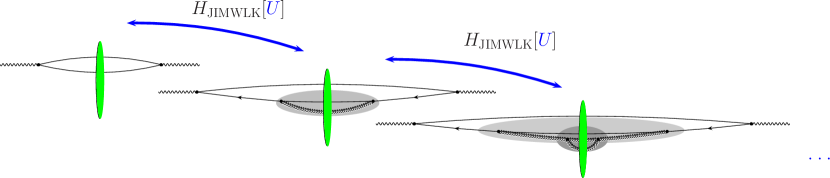
Figure 11: The JIMWLK operators adds gluons into the photon wavefunction, virtual corrections are not shown

To do so, one needs to write the evolution equation for a general correlator $O[U]$. To explore the first step shown in Fig.11, one might choose $O[U]$ to be

$$\hat{S}_{\bm{xy}}={\rm tr}(U^{\dagger}_{\bm{x}}U_{\bm{y}})/N_{c}$$ (89a)

which appears in the top left “bare” diagram. For convenience, I also define a shorthand for its $$Y$$ dependent expectation value

$$S_{Y;\bm{xy}}:=\langle\hat{S}_{\bm{xy}}\rangle_{Y}\ .$$ (89b)

To obtain the evolution equation, one simply multiplies both sides of (81) with $O[U]$ and averages with (80). The result then is an evolution equation for $\langle O[U]\rangle_{Y}$

$$\partial_{Y}\langle O[U]\rangle_{Y}=-\langle H_{\text{JIMWLK}}O[U]\rangle_{Y}\ .$$ (90)

Because of the nonlinear nature of $H_{\text{JIMWLK}}$ the r.h.s. will in no case be expressible by $\langle O[U]\rangle_{Y}$ alone, but instead involves other correlators as well. The evolution equation of these new quantities will then also be needed, and the argument repeats itself, ultimately leading to an infinite coupled hierarchy of evolution equations, the Balitsky hierarchy. For $\hat{S}_{\bm{xy}}$, one immediately arrives at

$$\partial_{Y}\big{\langle}\hat{S}_{\bm{xy}}\big{\rangle}_{Y}= \frac{\alpha_{s}}{2\pi^{2}}\Big{\langle}\Big{[}{\cal K}_{\bm{u}\bm{z}\bm{v}}\Big{(}i\nabla^{a}_{{\bm{u}}}i\nabla^{a}_{{\bm{v}}}+i\bar{\nabla}^{a}_{{\bm{u}}}i\bar{\nabla}^{a}_{{\bm{v}}}\Big{)}+{\cal K}_{\bm{u}\bm{z}\bm{v}}\Big{(}\big{[}\tilde{U}_{\bm{z}}\big{]}^{ab}(i\bar{\nabla}^{a}_{{\bm{u}}}i\nabla^{b}_{{\bm{v}}}+i\bar{\nabla}^{a}_{{\bm{v}}}i\nabla^{b}_{{\bm{u}}})\Big{)}\Big{]}\frac{{\rm tr}(U_{\bm{x}}U^{\dagger}_{\bm{y}})}{N_{c}}\Big{\rangle}_{Y}$$

$$= \frac{\alpha_{s}}{2\pi^{2}}\Big{\langle}\Big{[}\tilde{\cal K}_{\bm{x}\bm{z}\bm{y}}\Big{(}-2C_{\text{f}}\frac{{\rm tr}(U_{\bm{x}}U^{\dagger}_{\bm{y}})}{N_{c}}\Big{)}+\tilde{\cal K}_{\bm{x}\bm{z}\bm{y}}\ \frac{\big{[}\tilde{U}_{\bm{z}}\big{]}^{ab}2\ {\rm tr}(t^{a}U_{\bm{x}}t^{b}U^{\dagger}_{\bm{y}})}{N_{c}}\Big{]}\Big{\rangle}_{Y}$$ (91)

where

$$\tilde{\cal K}_{\bm{x}\bm{z}\bm{y}}=\big{(}2{\cal K}_{\bm{x}\bm{z}\bm{y}}-{\cal K}_{\bm{x}\bm{z}\bm{x}}-{\cal K}_{\bm{y}\bm{z}\bm{y}}\big{)}\ .$$ (92)

Observe on the r.h.s. the operator $\big{[}\tilde{U}_{\bm{z}}\big{]}^{ab}2\ {\rm tr}(t^{a}U_{\bm{x}}t^{b}U^{\dagger}_{\bm{y}})$ already anticipated in the corresponding discussion of Sec. 1.2. This term corresponds to the real contribution shown in the middle diagram of Fig. 11, while the other term is a virtual contribution not explicitly shown. I will return to explore this viewpoint in more detail in Sec. 5

To compare with the factorizing limit and in particular the BK equation, one applies the Fierz identity

$$\big{[}\tilde{U}_{\bm{z}}\big{]}^{ab}{\rm tr}(t^{a}U_{\bm{x}}t^{b}U^{\dagger}_{\bm{y}})=\frac{1}{2}\Big{(}{\rm tr}(U_{\bm{x}}U^{\dagger}_{\bm{z}}){\rm tr}(U_{\bm{z}}U^{\dagger}_{\bm{y}})-\frac{1}{N_{c}}{\rm tr}(U_{\bm{x}}U^{\dagger}_{\bm{y}})\Big{)}$$ (93)

to rewrite Eq. (3.2) as

$$\partial_{Y}\langle\hat{S}_{\bm{xy}}\rangle_{Y}=\frac{\alpha_{s}N_{c}}{2\pi^{2}}\int d^{2}z\ \tilde{\cal K}_{\bm{x}\bm{z}\bm{y}}\,\langle\hat{S}_{\bm{xz}}\hat{S}_{\bm{zy}}-\hat{S}_{\bm{xy}}\rangle_{Y}\ .$$ (94)

Alternatively in terms of

$$N_{Y;\bm{xy}}=\langle\hat{N}_{\bm{xy}}\rangle_{Y}\ ,\hskip 56.9055pt\hat{N}_{\bm{xy}}={\rm tr}(1-U^{\dagger}_{\bm{x}}U_{\bm{y}})/N_{c}$$ (95)

this equation reads

$$\partial_{Y}\langle{\hat{N}}_{\bm{xy}}\rangle_{Y}=\frac{\alpha_{s}N_{c}}{2\pi^{2}}\int\!\!d^{2}z\ \tilde{\cal K}_{\bm{x}\bm{z}\bm{y}}\,\Big{\{}\big{\langle}{\hat{N}}_{\bm{xz}}+{\hat{N}}_{\bm{zy}}-{\hat{N}}_{\bm{xy}}\big{\rangle}_{Y}-\big{\langle}{\hat{N}}_{\bm{xz}}{\hat{N}}_{\bm{zy}}\big{\rangle}_{Y}\Big{\}}$$ (96)

These immediately reduce to a closed equation for $S_{\bm{xy}}$ or $N_{\bm{xy}}$ respectively, if one assumes factorization in the nonlinearity on the r.h.s. by replacing

$$\langle\hat{S}_{\bm{xz}}\hat{S}_{\bm{zy}}\rangle_{Y}\to S_{Y;\bm{xz}}\>S_{Y;\bm{zy}}\hskip 28.45274pt\text{or equivalently}\hskip 28.45274pt\langle\hat{N}_{\bm{xz}}\hat{N}_{\bm{zy}}\rangle_{Y}\to N_{Y;\bm{xz}}\>N_{Y;\bm{zy}}\ .$$ (97)

The result is known as the BK equation and typically written in terms of $N_{Y;\bm{xy}}$:

$$\partial_{Y}N_{Y;\bm{xy}}=\frac{\alpha_{s}N_{c}}{2\pi^{2}}\int\!\!d^{2}z\ \tilde{\cal K}_{\bm{x}\bm{z}\bm{y}}\,\Big{\{}N_{Y;\bm{xz}}+N_{Y;\bm{zy}}-N_{Y;\bm{xy}}-N_{Y;\bm{xz}}N_{Y;\bm{zy}}\Big{\}}\ .$$ (98)

To come back to the Balitsky hierarchy, there are several equivalent options on how to write the next equation in the hierarchy built on top of $N_{Y;\bm{xz}}$ if factorization does not hold in Eq (96). One may consider the evolution equation of $\langle\hat{N}_{\bm{xz}}\hat{N}_{\bm{zy}}\rangle_{Y}$ or $\langle\hat{S}_{\bm{xz}}\hat{S}_{\bm{zy}}\rangle_{Y}$ as well as $\langle\big{[}U_{\bm{z}}\big{]}^{ab}2\ {\rm tr}(t^{a}U_{\bm{x}}t^{b}U^{\dagger}_{\bm{y}})\rangle_{Y}$ or any other combination on the r.h.s. of this “pre-BK equation.” In any case, $H_{\text{JIMWLK}}$ as given in (88) allows to arrive at these equations most efficiently.

3.3 General properties of JIMWLK and the fixed point at infinite energy

There are a number of quite general properties which have been shown to hold already on the JIMWLK level [13]. The most generic of these concerns the interpretation of the JIMWLK equation in a probabilistic sense. Due to the fact that the r.h.s. can be viewed as a total derivative (c.f. Eq. (78)), or equivalently by looking at Eq. (90) with $O[U]=1$, one finds that “probabilities” (the normalization of $\hat{Z}_{Y}[U]$) are conserved:

$$\partial_{Y}\int\hat{D}[U]Z_{Y}[U]=0\ .$$ (99)

In [13] it has been shown that the Fokker-Planck Hamiltonian in the JIMWLK equation is positive semidefinite. This leads to stable asymptotic behavior: a finite evolution step is given by

$$\hat{Z}_{Y}[U]=e^{-H_{\mathrm{JIMWLK}}(Y-Y_{0})}\hat{Z}_{Y_{0}}[U]\ ,$$ (100)

which, given positivity, means that evolution slowly erases high lying modes. The lowest lying mode, the solution with zero eigenvalues, on the other hand, is simply $\hat{Z}_{Y}[U]=1$, as the Fokker-Planck Hamiltonian Eq. (88) acts with at least one derivative. This solution acts therefore as the fixed point at $Y=\infty$ and carries the (conserved) normalization of all these “states.” This state then acts as a fixed point of evolution at infinite energy. In this situation ($\hat{Z}_{Y}[U]=1$) all there is to define correlators is the Haar measure, which acts locally in each point in transverse space. A first implication is that the correlation length in this situation is strictly zero. A second one is the fact that, via Eq. (100) the system moves toward this solution – in RG parlance this solution acts as an attractive fixed point. This is fully in line with the physics expectations laid out in the introduction: going to higher and higher energy adds more and more gluons of the same size, increases density and necessarily leads to a shrinking correlation length. This element of the physics picture then is already visible on the abstract level of positivity of the spectrum and existence of an attractive fixed point in this evolution equation.

3.4 Geometric scaling in BK and JIMWLK – the idea

At this point one is in a position to make first contact with the scaling idea of Golec-Biernat and Wüsthoff that provides such an efficient parametrization of the small ${x_{\text{bj}}}$ HERA data. The argument is due to Iancu, Itakura, and McLerran [55]. They assume (in the context of the fixed coupling BK equation just derived) that $N_{Y\ \bm{xy}}$ depends only on the combination $(\bm{x}-\bm{y})^{2}Q_{s}(Y)^{2}=:\bm{r}^{2}Q_{s}(Y)^{2}$. Then $Y$-derivatives can be traded for $\bm{r}^{2}$ derivatives and the l.h.s. of the BK equation is easily rewritten as

$$\partial_{Y}N({\bm{r}^{2}Q_{s}(Y)^{2}})=\bm{r}^{2}\partial_{\bm{r}^{2}}N({\bm{r}^{2}Q_{s}(Y)^{2}})\partial_{Y}\ln Q_{s}(Y)^{2}=:\bm{r}^{2}\partial_{\bm{r}^{2}}N({\bm{r}^{2}Q_{s}(Y)^{2}})2\lambda(Y)\ ,$$ (101)

where the last equality defines a new quantity, the evolution rate $\lambda(Y)=\partial_{Y}\ln Q_{s}(Y)$. Taking into account the spatial boundary conditions imposed by “color transparency+saturation,” i.e. the fact that $N(\bm{r}^{2}=0)=0$ and $N(\bm{r}^{2}=\infty)=1$, allows to take the zeroth moment of the BK equation –to integrate with $\frac{d^{2}r}{\bm{r}^{2}}$– in order to isolate $\lambda$ on the l.h.s.. The r.h.s then provides an integral expression for it in form of its zeroth moment:

$$2\pi\lambda(Y)=\frac{\alpha_{s}N_{c}}{2\pi^{2}}\int\frac{d^{2}rd^{2}z}{\bm{u}^{2}\bm{v^{2}}}\big{(}N(\bm{u}^{2}Q_{s}^{2})+N(\bm{v}^{2}Q_{s}^{2})-N(\bm{r}^{2}Q_{s}^{2})-N(\bm{u}^{2}Q_{s}^{2})N(\bm{v}^{2}Q_{s}^{2})\big{)}$$ (102)

where I have set $\bm{u}=\bm{x}-\bm{z}$ and $\bm{v}=\bm{z}-\bm{y}$ for compactness. Due to scale invariance of the integral, the r.h.s. is indeed independent of $Y$: the scale common to all $N$ can be chosen at will without changing the integral, $\lambda$ is constant. Using the definition of $\lambda$ in Eq. (101), this $Y$ independence of $\lambda$ immediately implies that $Q_{s}$ grows like a power in ${x_{\text{bj}}}$:

$$Q_{s}(Y)=e^{\lambda(Y-Y_{0})}Q_{s}(Y_{0})=\Big{(}\frac{{x_{\text{bj}}}_{0}}{{x_{\text{bj}}}}\Big{)}^{\lambda}Q_{s}({x_{\text{bj}}}_{0})\ .$$ (103)

This simple power like growth induced by constant $\lambda$ only holds at fixed coupling. Running coupling effects render $\lambda$ $Y$ dependent and thus modify the $Y$ dependence of $Q_{s}$ with the general trend to slow down evolution. These effects will be discussed in detail later on. For the moment, let me return to the implications of scaling features in small ${x_{\text{bj}}}$ evolution equations as such: if such scaling is to occur, the shape of the solution to the BK equation is strongly constrained – one has to simultaneously satisfy the scaling condition and the evolution equation. These combined requirements should be sufficient to completely fix the shape of the scaling solution in $\bm{r}$, a conclusion that has been confirmed by numerical work again and again.

The above argument only applies if the scaling situation is ever reached in evolution. Recently, Munier and Peschanski [56, 57, 58] have argued analytically that this feature should be attractive and emerge quite generally as soon as the “color transparency+saturation” condition is met on the initial condition. This was done using an approximation that maps the BK equation onto equations of the type of the Fisher and Kolmogorov-Petrovsky-Piscounov (KPP) equation [59, 60] which are known to posses “traveling wave” solutions which in this context appears as scaling. While numerical work on the BK equation had demonstrated this earlier on for certain initial conditions [61, 62, 63, 64, 65, 66, 67, 68, 69] this is a nice theoretical confirmation despite the need for an additional approximation.

This has very important implications: If such a regime is reached, the situation is qualitatively different from the situation encountered, say, in the case of DGLAP evolution. There, features of the initial conditions and the noncalculable nonperturbative information contained therein will be slowly washed out but never completely forgotten. In the scaling regime everything is determined by the (perturbatively calculated) evolution equation – the nonperturbative input of the initial condition is completely forgotten in the sense that it is sufficient to state that scaling is reached and that the saturation scale has a given value to fully determine the system at this and all further $Y$. The initial condition will be visible only before one enters the scaling regime and will determine the $Q_{s}$ value at which scaling initially emerges, but has no further influence on the evolution beyond that point. That this behavior is characteristic for this type of evolution equation, also in the more general JIMWLK case, has been explored extensively in numerical simulations [35] and will be further discussed in Sec. 6.

The discussion above applies to the BK equation, but it can be equally applied to the JIMWLK equation: With the scaling dimension of the $U$ fields at $1$, all the above scaling arguments go through, if one assumes all correlators of $U$ fields to carry $Y$-dependence only via $Q_{s}(Y)$. In principle this is not impossible and might emerge from evolution in a natural way, but it is easy to envision that it is at least violated in a particular physics situation via the initial condition to evolution. This should then be seen in experimental data over a certain range of ${x_{\text{bj}}}$ values.

The experimental implications are also striking. As an example consider the DIS cross section of Eq.(4). If the dipole cross section depends on $Y$ via $Q_{s}$ only, one should expect the DIS cross section to scale with $Q/Q_{s}(Y)$ as discussed in Sec. 8.1. This is the phenomenon originally called geometric scaling [34].

3.5 From JIMWLK and BK to BFKL, large $N_{c}$ and density expansions

Another important result is the statement that the BFKL equation emerges as the small density limit of the JIMWLK (and as a corollary, also of the BK) equation. This was first demonstrated in [8]. The argument involves an expansion of the dipole correlators $\langle N_{\bm{xy}}\rangle_{Y}$ in powers of the gluon field and thus in terms of gluon densities. As a consequence the nonlinear terms in Eq. (96) become negligible, and it turns out that Fourier-transforming the remainder leads directly to the BFKL equation. To state precisely what the expansion parameter for this low density limit may be, it is sufficient to consider the ansatz (33) and to rephrase the BK equation in terms of ${\cal G}$. Since ${\cal G}$ is a two gluon correlator, it is then easy to see that the low density expansion can be made precise as an expansion in powers of ${\cal G}$. The name density expansion is justified in the sense that ${\cal G}$ also fully determines the gluon density as seen from Eq. (43), but one has to remember that large ${\cal G}$ does not literally translate into large gluon densities.

The evolution I want to consider is in fact the evolution equation for the two point function before factorization into the BK form proper, i.e. Eq. (94), which I write explicitly as

$$\partial_{Y}\langle{\rm tr}(U_{\bm{x}}U^{\dagger}_{\bm{y}})\rangle=\frac{\alpha_{s}}{2\pi^{2}}\int\!\!d^{2}z\ \tilde{\cal K}_{\bm{xzy}}\Big{(}-2C_{\text{f}}\ \langle{\rm tr}(U_{\bm{x}}U^{\dagger}_{\bm{y}})\rangle+\langle\big{[}\tilde{U}_{\bm{z}}\big{]}^{ab}2{\rm tr}(t^{a}U_{\bm{x}}t^{b}U^{\dagger}_{\bm{y}})\rangle\Big{)}\ .$$ (104)

With the two point averages already known from Eq. (35a) all that is left to calculate is the three point function. This can be calculated along the same lines as the various two point functions. One finds

$$\langle[\tilde{U}_{\bm{z}}]^{ab}\ 2{\rm tr}(t^{a}U_{\bm{x}}t^{b}U^{\dagger}_{\bm{y}})\rangle=2N_{c}C_{\text{f}}e^{-\frac{1}{2}\big{(}N_{c}({\cal G}_{Y,{\bm{xz}}}+{\cal G}_{Y,{\bm{yz}}})-\frac{{\cal G}_{Y,{\bm{xy}}}}{N_{c}}\big{)}}\ .$$ (105)

Instead of an explicit construction let it suffice here that this result satisfies all necessary limiting relations. Using, where needed, the Fierz identity (93) one gets coincidence limits for the fields that have to be respected also for their correlators:

$$\lim\limits_{y\to z}\big{[}\tilde{U}_{\bm{z}}\big{]}^{ab}\ 2{\rm tr}(t^{a}U_{\bm{x}}t^{b}U^{\dagger}_{\bm{y}})= 2C_{\text{f}}\ {\rm tr}(U_{\bm{x}}U^{\dagger}_{\bm{z}})$$ (106a)

$$\lim\limits_{y\to x}\big{[}\tilde{U}_{\bm{z}}\big{]}^{ab}\ 2{\rm tr}(t^{a}U_{\bm{x}}t^{b}U^{\dagger}_{\bm{y}})= \tilde{\rm tr}(\tilde{U}_{\bm{x}}\tilde{U}^{\dagger}_{\bm{z}})$$ (106b)

$$\lim\limits_{x,y\to z}\big{[}\tilde{U}_{\bm{z}}\big{]}^{ab}\ 2{\rm tr}(t^{a}U_{\bm{x}}t^{b}U^{\dagger}_{\bm{y}})= 2N_{c}C_{\text{f}}\ .$$ (106c)

Obviously Eqns. (35) and (105) are compatible with these requirements.

Incidentally this truncates the nonlinear equation for the correlators of $U$ to a single, highly nonlinear equation for ${\cal G}$. Using the above, Eq. (104) reads

$$\partial_{Y}e^{-C_{\text{f}}{\cal G}_{Y,\bm{xy}}}=\frac{\alpha_{s}}{2\pi^{2}}\int\!\!d^{2}z\ \tilde{\cal K}_{\bm{xzy}}\Big{(}-2C_{\text{f}}e^{-C_{\text{f}}{\cal G}_{Y,\bm{xy}}}+2C_{\text{f}}e^{-\frac{1}{2}\big{(}N_{c}({\cal G}_{Y,{\bm{xz}}}+{\cal G}_{Y,{\bm{yz}}})-\frac{{\cal G}_{Y,{\bm{xy}}}}{N_{c}}\big{)}}\Big{)}$$

or, equivalently,

$$\partial_{Y}{\cal G}_{Y,\bm{xy}}=\frac{\alpha_{s}}{\pi^{2}}\int\!\!d^{2}z\ \tilde{\cal K}_{\bm{xzy}}\Big{(}1-e^{-\frac{N_{c}}{2}\big{(}{\cal G}_{Y,{\bm{xz}}}+{\cal G}_{Y,{\bm{yz}}}-{\cal G}_{Y,{\bm{xy}}}\big{)}}\Big{)}\ .$$ (107)

Since one involves only planar diagrams in the construction of the correlators due to locality of the weight in $Y$, one might have reached this result also via a different route: One rewrites the bracketed expression on the r.h.s of (104) once more using the Fierz identity (93) to map it onto the form given already in (96). Now one may factorize the nonlinearity in $\hat{N}$ in the large $N_{c}$ spirit to obtain the BK equation proper. Then one only needs to introduce an exponential parametrization of the form (35a), without any reference to the Gaussian weight of Eq. (33) at all and approximate $C_{\text{f}}\to N_{c}/2$ to arrive again at (107). This highlights the link of the BK equation with the large $N_{c}$ expansion quite clearly and demonstrates that (107) is fully equivalent to the more common forms of the BK equations shown earlier.

It is important to note that at this point one has strictly speaking left the realm of the original MV model with its assumption of uncorrelated scattering centers in longitudinal direction. Aside from the initial condition, ${\cal G}$, as it emerges as a solution to (107), will no longer scale with $A^{1/3}$. This will be discussed further in Sec. 7.2.

For small ${\cal G}$ (107) immediately reduces to the coordinate space BFKL equation in the form

$$\partial_{Y}{\cal G}_{Y,\bm{xy}}=\frac{\alpha_{s}N_{c}}{2\pi^{2}}\int\!\!d^{2}z\ \tilde{\cal K}_{\bm{xzy}}\big{(}{\cal G}_{Y,{\bm{xz}}}+{\cal G}_{Y,{\bm{yz}}}-{\cal G}_{Y,{\bm{xy}}}\big{)}\ .$$ (108)

That this equation indeed relates to the better kown momentum space version requires a little work, but the correspondence is expected: it has been demonstrated for the forward limit of the JIMWLK and BFKL equations already in [8]. Recently, Bartels, Lipatov and Vacca [70] have shown explicitly that the lowest order part of (107) corresponds to the full non-forward BFKL equation (at leading order in $\ln(1/{x_{\text{bj}}})$). Since this equation is usually written for a gluon 4-point function, this requires an explanation.

In this low density limit, all that Eq. (107) does is to iterate the BFKL variant of what is called reggeized two gluon exchange between projectile and target. This allows to draw both sides more symmetrically than in Eqns. (37) and (38) and to expose the two coordinates (labelled $\bm{u}$ and $\bm{v}$ below) at which the exchanged pair of gluons couples to the target. This corresponds to the step from a the solution of a Bethe Salpeter type equation to the corresponding Greens function. This latter object will be denoted ${\cal G}_{Y;\ \bm{xy},\bm{uv}}$, with Fourier-transform $\delta^{(2)}({\bm{q}}-{\bm{q}}^{\prime})\Phi_{Y}({\bm{k}},{\bm{k}}^{\prime};{\bm{q}}^{\prime})$. Diagrammatically, this is written as

$${\cal G}_{Y;\ \bm{xy},\bm{uv}}=\parbox{85.35826pt}{ \includegraphics[height=71.13188pt]{G-4-coords}}\hskip 28.45274pt\Phi_{Y}({\bm{k}},{\bm{k}}^{\prime};{\bm{q}}^{\prime})=\parbox{85.35826pt}{ \includegraphics[height=71.13188pt]{G-4-moms}}\ .$$ (109)

[The definition in terms of underlying gluon correlators now contains local subtractions of the type shown in (38) both for top and bottom coordinates.] Explicitly, with this assignment of variables

$$\delta^{(2)}({\bm{q}}-{\bm{q}}^{\prime})\Phi_{Y}({\bm{k}},{\bm{k}}^{\prime};{\bm{q}}^{\prime})=\int d^{2}x\,d^{2}y\,d^{2}u\,d^{2}v\ {\cal G}_{Y;\ \bm{xy},\bm{uv}}\ e^{i{\bm{k}}{\bm{x}}+i({\bm{q}}-{\bm{k}}){\bm{y}}-i{\bm{k}}^{\prime}{\bm{u}}-i({\bm{q}}^{\prime}-{\bm{k}}^{\prime}){\bm{v}}}$$ (110)

and to make contact with the standard momentum space formulation reduces to a simple exercise in Fourier transformation.

The connection between the result of these manipulations and the conformal formulation in coordinate space is well documented in the literature so that taking this route might be easier to the non-expert than the direct calculation of [70]. Only by using conformal symmetry tools is it possible to write complete solutions to the nonforward BFKL equation – but this is outside the scope of this review.

While the authors in [70] arrive at the BFKL limit in the usual way, by simply dropping the nonlinearity in Eq. (96), and hence refer to $N$ as the object of their evolution equation their calculations make it clear that they discuss a two gluon object coupling to the photon wavefunction or “impact factor.” This object has to be identified with ${\cal G}$ as done above.

The form of the nonlinearity in Eq. (107) is intriguing in its exponential nature. This directly corresponds to the eikonal nature of the multiple scattering induced by the presence of complete Wilson lines in the definition of correlators $S_{Y;{\bm{xy}}}$ or $N_{Y;{\bm{xy}}}$. This becomes important as soon as one attempts to go beyond leading order in density, as becomes necessary if one tries to step beyond the large $N_{c}$ limit. For example [70] aims at providing a $1/N_{c}$ correction to the BK equation. They find a contribution which contains the square of $\frac{N_{c}}{2}\big{(}{\cal G}_{Y,{\bm{xz}}}+{\cal G}_{Y,{\bm{yz}}}-{\cal G}_{Y,{\bm{xy}}}\big{)}$, the factor in the exponent of the ($N_{c}$-leading) expression (107). If the eikonalization feature of JIMWLK and BK equations is taken seriously, this can not be done in a way consistent with the density expansion without also including higher order contributions from the nonlinearity on the r.h.s. of (107). At least for large nuclei this becomes an important consideration.

3.6 Growth in BFKL and BK, the Mueller-Triantafyllopoulos description

To identify BFKL as the low density limit of JIMWLK and BK implies that linear BFKL evolution is present in the more general framework and should manifest itself in those areas of phase space in which densities are not yet large. BFKL is known for fast and unlimited growth of its solutions, the ${\cal G}$ or $\Phi$ above. The role of the nonlinear effects is clearly to tame this growth and to ensure that the objects of evolution, $S_{Y;{\bm{xy}}}$ or $N_{Y;{\bm{xy}}}$ for example, with their interpretation as correlators of eikonal factors $U_{\bm{x}}^{(\dagger)}$ stay bounded between $0$ and $1$.

Mueller and Triantafyllopoulos [73, 74] have provided a very elucidating perspective on this matter that employs BFKL as the driving force behind all growth at small ${x_{\text{bj}}}$ which turns out to be surprisingly successful. The ideas entering this model naturally incorporate the notion of a scaling window [55] – a region in phase space at distances shorter than $1/Q_{s}$, i.e. away from the high density limit, at which the presence of $Q_{s}$ exerts its influence.

As indicated, one cornerstone of these ideas is the strong growth and diffusive character of BFKL evolution which can be most easily understood in the forward case (i.e. the above equation at $q=0$). At $q=0$ the above equations can be diagonalized by power functions

$$e^{(\nu,n)}({\bm{k}})=2\pi\sqrt{2}\,({\bm{k}}^{2})^{-\frac{3}{2}-i\nu}e^{-in\phi}\phantom{xx};\;\nu\in{\mathbb{R}},n\in{\mathbb{Z}}$$ (111)

in momentum- as well as in coordinate space. The eigenvalues are given by

$$\chi(\nu,n):=\frac{\alpha_{s}N_{c}}{\pi}\left[2\psi(1)-\psi(\frac{1+|n|}{2}+i\nu)-\psi(\frac{1+|n|}{2}-i\nu)\right]\ ;\hskip 56.9055pt\chi(\nu):=\chi(\nu,0)$$ (112)

with $\psi$ defined as the logarithmic derivative of the $\Gamma$-function ($\psi(x)=\Gamma^{\prime}(x)/\Gamma(x)$) and $\chi(\nu)$ as a shorthand for $\chi(\nu,0)$. The solution then reads

$$\Phi_{Y}({\bm{k}},{\bm{k}}^{\prime})=\sum_{n=-\infty}^{+\infty}\int_{-\infty}^{+\infty}\frac{d\nu}{2\pi}\ e^{(\nu,n)}({\bm{k}})\ e^{Y\chi(\nu,n)}\ e^{(\nu,n)\,\ast}({\bm{k}}^{\prime})\ .$$ (113)

Of particular interest is the large $Y$ asymptotics of this equation. There the contributions will be dominated by the modes with $n=0$, shown here in the coordinate space version to underline the analogy [28]:

$${\cal G}_{Y;\bm{xy},\bm{uv}}=\int\frac{d\nu}{2\pi^{2}}\ ((\bm{x}-\bm{y})^{2})^{-\frac{1}{2}+i\nu}e^{Y\chi(\nu)}((\bm{u}-\bm{v})^{2})^{-\frac{1}{2}-i\nu}=\int\frac{d\tilde{\nu}}{2\pi^{2}i}e^{Y\chi(\tilde{\nu})-(1-\tilde{\nu})(\rho-\rho^{\prime})}$$ (114)

where $\rho:=\ln(\bm{x}-\bm{y})^{2}\mu^{2}$ and $\rho^{\prime}:=\ln(\bm{u}-\bm{v})^{2}\mu^{2}$. The integration contour in the $\nu$ (or Mellin-) integral is to be taken parallel to the imaginary axis, to the right of all singularities; in the last version I have substituted $\tilde{\nu}:=i\nu$ with an appropriate change in definition of $\chi$.

Further insight emerges by taking the saddle point approximation to in Eq. (113) or (114). This selects $\nu_{0}=0$ as the extremal value in the $\nu$ integration. The result displays a factorizing structure,

$$e^{Y\chi({\tilde{\nu}}_{0})}\int\frac{d{\tilde{\nu}}}{2\pi^{2}i}e^{Y\frac{1}{2}\chi^{\prime\prime}({\tilde{\nu}}_{0})({\tilde{\nu}}-{\tilde{\nu}}_{0})^{2}+({\tilde{\nu}}-{\tilde{\nu}}_{0})(\rho-\rho^{\prime})}=e^{Y\chi({\tilde{\nu}}_{0})}\frac{1}{\sqrt{\chi^{\prime\prime}({\tilde{\nu}}_{0})Y}}e^{-\frac{(\rho-\rho^{\prime})^{2}}{\chi^{\prime\prime}({\tilde{\nu}}_{0})Y}}$$ (115)

where the first factor, $e^{Y\chi({\tilde{\nu}}_{0})}=\left(\frac{{x_{\text{bj}}}_{0}}{{x_{\text{bj}}}}\right)^{\chi({\tilde{\nu}}_{0})}$, describes the strong, power like growth in $1/{x_{\text{bj}}}$ alluded to already in the introduction. The second factor, which originates from the Gaussian integral in ${\tilde{\nu}}$, describes diffusion in the transverse plane of dipole sizes:

$$\psi_{Y}(\rho-\rho^{\prime}):=\frac{1}{\sqrt{\chi^{\prime\prime}({\tilde{\nu}}_{0})Y}}\ e^{-\frac{(\rho-\rho^{\prime})^{2}}{2\chi^{\prime\prime}({\tilde{\nu}}_{0})Y}}$$ (116)

is immediately recognizable as the solution to the diffusion equation

$$\partial_{Y}\psi_{Y}(\rho)=\frac{\chi^{\prime\prime}({\tilde{\nu}}_{0})}{2}\partial_{\rho}^{2}\psi_{Y}(\rho)$$ (117)

with initial condition $\psi_{0}(\rho)=\delta(\rho)$. The same picture holds in momentum space as well. This is the well known IR problem of the BFKL equation at one loop accuracy: even an initially short range configuration spreads to nonperturbatively large distances. Since the main focus here is in nonlinear effects I will refrain from a discussion of two loop corrections to BFKL.

This diffusion and growth now has to be contrasted with what happens in JIMWLK and BK evolution. The nonlinearity tames the growth and, at the same time, prevents diffusion into the infrared. At small ${\cal G}$, though, evolution is correctly described by BFKL dynamics.

Mueller and Triantafyllopoulos therefore have suggested to simulate the presence of the nonlinear term by an absorptive barrier in the above diffusion process that is to be self consistently adjusted such that the solution to the so modified BFKL equation never grows large. The result can be interpreted as a change of the dominant contributions to the integral in, say (114), in such a way that one now follows the saddle point but allows diffusion only from small dipoles at size ranges where ${\cal G}$ is not yet large. Creation of new objects in the already saturated domain is eliminated via absorption across the boundary.

In order to explore the first part of this argument and to understand how to choose the absorptive boundary, one can look for directions in $Y-Q$ phase space in which BFKL evolution remains bounded by simultaneously looking for a saddle point and $Y$ dependent starting sizes $\rho^{\prime}(Y)$, for which the exponent in Eq. (114) vanishes and thus ${\cal G}$ remains approximately constant [73, 55]. The conditions to satisfy in this case are

$$Y\chi^{\prime}(\tilde{\nu}_{c})+(\rho-\rho^{\prime}(Y))=0$$ saddle point (118a)

$$Y\chi(\tilde{\nu}_{c})+(1-\tilde{\nu}_{c})(\rho-\rho^{\prime}(Y))=0 \hskip 28.45274pt\text{(almost) const. }{\cal G}$$ (118b)

with solutions

$$\frac{\chi^{\prime}(\tilde{\nu}_{c})}{\chi(\tilde{\nu}_{c})}= \frac{1}{1-\tilde{\nu}_{c}}$$ (119a)

$$\rho-\rho^{\prime}(Y)= \frac{\chi(\tilde{\nu}_{c})}{1-\tilde{\nu}_{c}}Y\ .$$ (119b)

(The saddle point value $$\tilde{\nu}_{c} \tilde{\nu}_{0} \rho=:\ln(r^{2}\mu^{2}) \rho^{\prime}(Y)=:\ln R_{0}^{2}(Y)\mu^{2}$$ remains implicit, but changes slightly from the BFKL value .) Translating the latter back into distances and one finds

$$R_{0}^{2}(Y)= r^{2}e^{-\frac{\chi(\tilde{\nu}_{c})}{1-\tilde{\nu}_{c}}Y}\ .$$ (119c)

Using this as a saddle point for the integral in ${\cal G}$ one finds

$${\cal G}_{Y;r,R_{0}(Y)}\approx \left(\frac{r^{2}}{R_{0}(Y)}\right)^{(1-{\tilde{\nu}}_{c})}\int\frac{d{\tilde{\nu}}}{2\pi^{2}i}e^{Y\frac{1}{2}\chi^{\prime\prime}({\tilde{\nu}}_{c})({\tilde{\nu}}-{\tilde{\nu}}_{c})^{2}+({\tilde{\nu}}-{\tilde{\nu}}_{c})\ln\left(\frac{r^{2}}{R_{0}(Y)}\right)}$$

$$= \left(\frac{r^{2}}{R_{0}(Y)^{2}}\right)^{(1-{\tilde{\nu}}_{c})}\frac{e^{-\frac{(\rho-\rho^{\prime})^{2}}{\chi^{\prime\prime}({\tilde{\nu}}_{c})Y}}}{\sqrt{\chi^{\prime\prime}({\tilde{\nu}}_{c})Y}}\ .$$ (120)

A list of observations apply [73]:

• Within the diffusion radius the dominant factor is $\left(r^{2}/R_{0}(Y)\right)^{(1-{\tilde{\nu}}_{c})}$. The solution has scaling form, just as argued above for the solutions of the JIMWLK and BK equations after some initial settling down. The scale variable is $R_{0}$ which has exponential $Y$ dependence, again as required in the BK case. Moreover the coefficient is known from Eq. (119).

• Apart from a mild correction through the square root factor, $R_{0}(Y)$ describes lines of constant ${\cal G}$. ${\cal G}$ evolved in this manner will not grow exponentially. This is because emission from large objects has been prohibited in sharp contrast to the diffusion of the BFKL equation.

Of course the argument can be equally phrased in momentum space which essentially replaces $r\to 1/Q$ and $R_{0}\to 1/Q_{0}$.

One may remove the nonscaling square root factor by replacing condition (118b), with the requirement of truly constant $\cal G$ and work with the resulting definition of $Q_{0}\to Q_{s}$ without introducing absorptive boundaries. However, evolution speed $\lambda=\partial_{Y}\ln Q_{s}$, will necessarily change if one really implements the effect of the nonlinearity in form of the absorptive boundary. Mueller and Triantafyllopoulos [73, 74] continue to formalize their argument by also including running coupling effects. In their treatment, the scale for the coupling is set by the size of the emitting object, the parent “dipole.” These refinements do not change the generic conclusions given above but they ensure scaling and provide quantitative results for $\lambda$ and $Q_{s}$. Due to the approximations made, their results are valid asymptotically at large $Y$ and contain an unknown constant (called $\tilde{Y}$ below) which is related to the (uncontrolled) small $Y$ details. I write their result for the evolution as in [35]:

$$\lambda:=\partial_{Y}\ln Q_{s}(Y)=\frac{.90}{\sqrt{Y+\tilde{Y}}}-\frac{0.47}{(Y+\tilde{Y})^{5/6}}+\text{higher inverse powers}\ .$$ (121)

This can be integrated to give $Q_{s}$ at the price of an additional integration constant $\tilde{c}$:

$$\frac{Q_{s}(Y)}{\Lambda_{\text{QCD}}}=\tilde{c}\cdot\exp[2\cdot 0.9(Y+\tilde{Y})^{\frac{1}{2}}-6\cdot 0.47(Y+\tilde{Y})^{\frac{1}{6}}]\ .$$ (122)

In particular the coefficient of the second term is affected by the presence of the absorptive boundary. Its value will turn out to be important in the comparison with numerical simulations shown in Fig. 23.

Clearly running coupling effects do slow down evolution quite considerably, the leading contribution goes from an exponent linear in $Y$ to a square root in the exponent but they do not destroy scaling. The functional form of the diffusive factor in Eq. (3.6) is modified through the correct determination of lines of constant ${\cal G}$ but functional form of the leading $\left(Q^{2}/Q_{s}(Y)^{2}\right)^{-(1-{\tilde{\nu}}_{c})}$ is unaltered (although ${\tilde{\nu}}_{c}$ changes slightly from the solution to (119)) [73]:

$${\cal G}_{Y;Q,Q_{s}(Y)}=C\left(\frac{Q^{2}}{Q_{s}(Y)^{2}}\right)^{-(1-{\tilde{\nu}}_{c})}\left[\ln\frac{Q^{2}}{Q_{s}(Y)^{2}}+\frac{1}{1-{\tilde{\nu}}_{c}}\right]\ .$$ (123)

$\tilde{\nu}_{c}$ (or $\tilde{\nu}_{0}$ in pure BFKL) is usually called the anomalous dimension governing the leading large $k$ behavior of the unintegrated gluon distribution through (43). This result is expected to hold in what is called the scaling window which will be discussed next.

3.7 Scaling above $Q_{s}$, the existence of a scaling window

The scaling form of Eq.(123) is valid at small ${\cal G}$ which immediately implies distances shorter than $1/Q_{s}$. Consequently, one has to ask how far away from $Q_{s}$ this can be trusted. This, in fact, is important not only for the approximate solution discussed above but also as a limitation on the range of validity of the evolution equations, be it JIMWLK or BK. That this range is limited as a matter of principle should be clear from the derivation of these equations, which selects contributions of the form $\alpha_{s}\ln(1/{x_{\text{bj}}})$ and rejects contributions enhanced by other logarithms, such as $\alpha_{s}\ln(Q^{2}/\mu^{2})$ as subleading. If one looks at the phase space plot of Fig. 4, one would naively expect $\ln(1/{x_{\text{bj}}})$ corrections to be most important above the diagonal, while $\ln(Q^{2}/\mu^{2})$ corrections should be most important below the diagonal, with a region in between in which double logarithmic corrections of the form $\alpha_{s}\ln(1/{x_{\text{bj}}})\ln(Q^{2}/\mu^{2})$ are most important. But where can one safely neglect these other logarithms?

Even before Mueller and Triantafyllopoulos constructed their scaling solutions, [55] have in fact argued that the range of validity of the evolution equations and also of scaling expressions of the type (123) is surprisingly large. It is expected to extend over a large scaling window defined by the condition

$$Q_{s}^{2}\leq Q^{2}\leq Q_{s}^{4}/\Lambda_{\text{QCD}}^{2}$$ (124)

or, more stringently

$$1\lesssim\ln(Q^{2}/Q_{s}^{2})\ll\ln(Q_{s}^{2}/\Lambda_{\text{QCD}}^{2})\ .$$ (125)

The original argument is based on the diffusion radius of BFKL if one follows evolution along lines of (almost) constant $\cal G$ as in Eq.(3.6). This sets a natural range for the validity of scaling formulae like (123).

Besides the theoretical considerations above, the existence of a scaling window is also important phenomenologically. The key example is the G-B+W idea to fit the HERA data with a scaling ansatz. In the HERA range $Q_{s}$ comes out to lie in between $1-2$GeV², while the momenta entering the fit range extend up to $Q^{2}$ of several hundred GeV². Thus it is natural to expect these data to exhibit scaling features only if a scaling window exists that reaches far beyond $Q_{s}$. In a sense, the success of the G-B+W fit directly poses the question for the existence of such a window whose theoretical origin was only understood much later in [55].

4 Fokker-Planck and Langevin

At this point all of the regions marked in the phase space plot of Fig. 4 have been fully explained in terms of a QCD evolution equation although for some of the steps certain approximations have been used. To go beyond this stage numerical work is needed. To allow for an efficient numerical treatment of the JIMWLK equation a reformulation is required. This takes the form of a translation of the Fokker-Planck equation to a Langevin description. This is done in Secs. 4.1 and 4.2. Interestingly enough, in this process one finds theoretical tools that also help in interpreting the gluon radiation process and directly lead to the diagrammatic interpretation of Eq. (7). This step is performed in Sec. 4.3 while the interpretation will become clear only in Sec. 5 by way of a surprisingly close analogy with the theory of QCD jets.

4.1 From Fokker-Planck to Langevin: Illustrating the idea

Although this topic is covered in many textbooks, the presentation is often somewhat old-fashioned and the intimate connection with path-integrals is not always mentioned. For this reason I demonstrate the relationship of Fokker-Planck and Langevin formulations with the aid of a simple toy example, a particle diffusion problem, that, for ease of comparison, shares some of the features of our problem. The toy model equation is

$$\partial_{Y}P_{Y}(\bm{x})=-H_{\text{FP}}\ P_{Y}(\bm{x})$$ (126)

with a Fokker-Planck Hamiltonian

$$H_{\text{FP}}=\frac{1}{2}i\partial_{\bm{x}}^{\mu}\,\chi_{\mu\nu}(\bm{x})\,i\partial_{\bm{x}}^{\nu}\ .$$ (127)

The particle coordinates $\bm{x}$ (in $D$ dimensional space) correspond to the field variables of the original problem and the probability distribution $P_{Y}$ to $\hat{Z}_{Y}$. It serves to define correlation function of some operator $O(\bm{x})$ via $\langle O(\bm{x})\rangle_{Y}=\int d^{D}x\ O(\bm{x})P_{Y}(\bm{x})$.

Eq. (126) admits a path-integral solution which is, as usual, built up from infinitesimal steps in $Y$: this is a solution $P(Y^{\prime},\bm{x}^{\prime};Y,\bm{x})$ with initial condition

$$P(Y,\bm{x}^{\prime};Y,\bm{x})=\delta^{(D)}(\bm{x}^{\prime}-\bm{x})$$ (128)

that is composed of many, infinitesimally small steps at times $Y_{k}:=Y+k\epsilon$. In this solution, the product rule

$$P(Y^{\prime},\bm{x}^{\prime};Y,\bm{x})=\int d^{D}x_{n-1}\ldots d^{D}x_{1}\ P(Y^{\prime},\bm{x}^{\prime};Y_{n-1},\bm{x})P(Y_{n-1},\bm{x}_{n-1};Y_{n-2},\bm{x}_{n-2})\ldots P(Y_{1},\bm{x}_{1};Y,\bm{x})$$ (129)

expresses the finite $Y^{\prime}-Y$ solution $P(Y^{\prime},\bm{x}^{\prime};Y,\bm{x})$ in terms of infinitesimal steps $P(Y_{i},\bm{x}_{i};Y_{i-1},\bm{x}_{i-1})$. Arbitrary initial conditions $P_{Y_{0}}(\bm{x})$ are then recovered via $P_{Y}(\bm{x})=\int d^{D}yP(Y,\bm{x};Y_{0},\bm{y})P_{Y_{0}}(\bm{y})$.

The derivation of the infinitesimal step from $Y_{i-1}$ to $Y_{i}=Y_{i-1}+\epsilon$ is textbook material. It reads (the index $i$ on the coordinate also refers to the time step, not to the vector component)

$$P(Y_{i},\bm{x}_{i};Y_{i-1},\bm{x}_{i-1})=N\int\!\!d^{D}p_{i}\ e^{-\epsilon\big{(}\frac{1}{2}\bm{p}_{i}^{\alpha}\bm{p}_{i}^{\beta}\chi^{\alpha\beta}(\bm{x}_{i-1})+i\bm{p}_{i}\cdot\big{(}\frac{\bm{x}_{i}-\bm{x}_{i-1}}{\epsilon}-\sigma(\bm{x}_{i-1})\big{)}\big{)}}+{\cal O}(\epsilon^{2})$$ (130)

where $\sigma_{\mu}(\bm{x}):=\frac{1}{2}i\partial_{\bm{x}}^{\alpha}\chi_{\alpha\mu}(\bm{x})$ and $N$ is a coordinate independent normalization factor.

From here, the step to the Langevin formulation is trivial: as this expression is quadratic in the momenta one can trivially rewrite it with the help of an auxiliary variable $\bm{\xi_{i}}$ [$i$ again the step label] as

$$P(Y_{i},\bm{x}_{i};Y_{i-1},\bm{x}_{i-1})=N\int\!\!d^{D}\xi_{i}\ \sqrt{\det(\chi(\bm{x}_{i}))}\ e^{-\frac{1}{2}\bm{\xi}_{i}\chi^{-1}(\bm{x}_{i})\bm{\xi}_{i}}\ \delta^{D}\big{(}\bm{x}_{i}-[\bm{x}_{i-1}+\epsilon(\bm{\xi}_{i}+\sigma(\bm{x}_{i-1})]\big{)}\ .$$ (131)

The $\delta^{D}(\ldots)$ arises from the momentum integration and determines $\bm{x}_{i}$ in terms of $\bm{x}_{i-1}$ and the correlated noise $\bm{\xi}_{i}$. The equation for $\bm{x}_{i}$,

$$\bm{x}_{i}=\bm{x}_{i-1}+\epsilon\big{(}\bm{\xi}_{i}+\sigma(\bm{x}_{i-1})\big{)}\ ,$$ (132)

is called the Langevin equation. It contains both a deterministic term [the $\sigma(\bm{x}_{i-1})$ term] and a stochastic term [the $\bm{\xi}$ term]. To fully define the problem without any reference to its path-integral nature, one then needs to state the Gaussian nature of the (correlated) noise separately. This is the formulation often found in textbooks. The path-integral version would appear to be much more elucidating and up to date.

If, as in the JIMWLK case, $\chi$ factorizes as

$$\chi_{\mu\nu}(\bm{x})={\cal E}_{\mu a}(\bm{x}){\cal E}_{\nu a}(\bm{x})\ ,$$ (133)

a simple redefinition of the noise variable leads to a version of the Langevin formulation with a Gaussian white noise:

$$P(Y_{i},\bm{x}_{i};Y_{i-1},\bm{x}_{i-1})=N\int\!\!d^{n}\xi_{i}\ e^{-\frac{1}{2}\bm{\xi}_{i}^{2}}\ \delta^{D}\big{(}\bm{x}_{i}-[\bm{x}_{i-1}+\epsilon({\cal E}(\bm{x}_{i-1})\bm{\xi}_{i}+\sigma(\bm{x}_{i-1})]\big{)}\ .$$ (134)

The correlation is now absorbed into the Langevin equation through the appearance of ${\cal E}$ which reads

$$\bm{x}_{i}=\bm{x}_{i-1}+\epsilon\big{(}{\cal E}(\bm{x}_{i-1})\bm{\xi}_{i}+\sigma(\bm{x}_{i-1})\big{)}\ .$$ (135)

Wherever this form is available, it will be the most efficient version to use in a numerical simulation, as the associated white noise can be generated more efficiently than the correlated noise of the more general case.

What is left is to sketch a numerical procedure to implement the solution given in (129), (130) using the expressions Eq. (131) or Eq. (134). As a first step one replaces the average with the probability distribution $P_{Y}(\bm{x})$ by an ensemble average

$$\langle O(\bm{x})\rangle_{Y}=\int\!d^{D}x\ O(\bm{x})\ P_{Y}(\bm{x})\approx\frac{1}{N}\sum\limits_{U\in{\sf E}[P_{Y}]}O(\bm{x})$$ (136)

where $N$ is the size of the (large) ensemble which is taken according to the probability distribution $P_{Y}(\bm{x})$. This one can easily do for the initial condition at $Y_{0}$. The Langevin equation then allows to propagate each ensemble member in $Y$ by $\epsilon$, thereby providing a new ensemble at $Y_{1}=Y+\epsilon$. Iteration then creates a chain of ensembles for a discrete set of $Y_{i}$ that provide an approximation to a set of $P_{Y_{i}}(\bm{x})$ in that they allow one to measure any correlator $\langle O(\bm{x})\rangle_{Y}$ according to Eq. (136).

The above clearly shows that a “Langevin system” is a way to write a path-integral solution to a differential equation that is particularly easy to implement numerically. Many, often confusing issues, such as the time step discretization issues, find their natural resolution in this path integral setting.

4.2 A Langevin formulation for JIMWLK evolution

Translating Fokker-Planck equations to Langevin equations for numerical work is not only useful in the case of a particle system as portrayed in the previous subsection. Also in the case of the JIMWLK equation this is the only promising angle of attack. Besides the evolution “time”-discretization needed in any example, it is also necessary to discretize transverse space to render the number degrees of freedom finite. Similar methods have been discussed in lattice gauge theory under the general heading stochastic quantization.

In the present context, this approach has already been suggested in [13] and a derivation has been given in [75] to which I refer the reader for details. To affect the translation in analogy to the example above, one may follow [13] and write the JIMWLK equation as

$$\partial_{Y}\hat{Z}_{Y}[U] =-\nabla^{a}_{\bm{x}}\Big{[}\frac{1}{2}\nabla^{b}_{\bm{y}}\hat{\chi}^{ab}_{\bm{xy}}-\big{(}\frac{1}{2}\nabla^{b}_{\bm{y}}\hat{\chi}^{ab}_{\bm{xy}}\big{)}\Big{]}\hat{Z}_{Y}[U]$$ (137)

and define

$$\hat{\sigma}^{a}_{\bm{x}}:=\frac{1}{2}\nabla^{b}_{\bm{y}}\hat{\chi}^{ab}_{\bm{xy}}=-i\big{(}\frac{1}{2}\frac{\alpha_{s}}{\pi^{2}}\int\!\!d^{2}z\frac{1}{({\bm{x}}-{\bm{z}})^{2}}\tilde{\rm tr}(\tilde{t}^{a}\tilde{U}_{\bm{x}}^{\dagger}\tilde{U}_{\bm{z}})\Big{)}$$ (138)

(the “$\sim$” indicating adjoint matrices and traces).

One then abandons the description in terms of weight functionals $\hat{Z}_{Y}$ in favor of one in terms of ensembles of fields which are governed by the corresponding Langevin equations.

Explicitly, to calculate any observable $O[U]$ of the fields $U$ one writes

$$\langle O[U]\rangle_{Y}=\int\!\hat{D}[U]O[U]\hat{Z}_{Y}[U]\approx\frac{1}{N}\sum\limits_{U\in{\sf E}[\hat{Z}_{Y}]}O[U]$$ (139)

where, separately at each $Y$, the sum is over an ensemble ${\sf E}[\hat{Z}_{Y}]$ of $N$ configurations $U$ whose members were created randomly according to the distribution $\hat{Z}_{Y}$. Clearly, for $N\rightarrow\infty$, the ensemble and $\hat{Z}_{Y}$ contain the same information.

The Langevin equation then schematically reads

$$\partial_{Y}\,[U_{\bm{x}}]_{ij}=[U_{\bm{x}}it^{a}]_{ij}\Big{[}\int\!\!d^{2}y\,[{\cal E}_{\bm{x}\bm{y}}^{ab}]_{k}[\xi^{b}_{\bm{y}}]_{k}+\hat{\sigma}^{a}_{\bm{x}}\Big{]}$$ (140)

where

$${\cal E}^{ab}_{{\bm{x}}{\bm{y}}}=\left(\frac{\alpha_{s}}{\pi^{2}}\right)^{1/2}\frac{({\bm{x}}-{\bm{y}})_{k}}{({\bm{x}}-{\bm{y}})^{2}}[1-\tilde{U}^{\dagger}_{\bm{x}}\tilde{U}_{\bm{y}}]^{ab}$$ (141)

is the “square root” of $\chi$, $\chi^{ab}_{{\bm{x}}{\bm{y}}}={\cal E}^{ac}_{{\bm{x}}{\bm{z}}}{\cal E}^{cb}_{{\bm{z}}{\bm{y}}}$, and $\xi$ are independent Gaussian random variables with correlators determined according to

$$\langle\ldots\rangle_{\xi}=\int\!D[\xi]\,(\ldots)\,e^{-\frac{1}{2}\xi\xi}\ .$$ (142)

This clearly represents an equation for an infinitesimal change of an element of $SU(N_{c})$. In fact, the components of $\omega^{a}_{\bm{x}}:=\Big{[}\int\!\!d^{2}y\,[{\cal E}_{\bm{x}\bm{y}}^{ab}]_{k}[\xi^{b}_{\bm{y}}]_{k}+\hat{\sigma}^{a}_{\bm{x}}\Big{]}$ can be directly interpreted as the “angles” parametrizing a local gauge transformation in transverse space.

It is of particular importance to note that the possibility to formulate the stochastic term via a completely decorrelated Gaussian noise $\xi$, that is to say with $\langle\xi^{a,i}_{\bm{x}}\xi^{b,j}_{\bm{y}}\rangle=\delta^{ab}\delta^{ij}\delta^{(2)}_{\bm{x}\bm{y}}$, reduces the numerical cost for a simulation like this considerably.

All that is left to do conceptually is the explicit discretization and the creation of an initial condition in form of an ensemble of $U$ fields at $Y_{0}$.

A reasonable choice for the initial condition is an ensemble that leads to a shape for $\langle U^{\dagger}_{\bm{x}}U_{\bm{y}}\rangle$ that is compatible with the generic physics requirements as shown in Fig. 7, for instance with

$$\langle U^{\dagger}_{\bm{x}}U_{\bm{y}}\rangle\propto\exp\left(\frac{-({\bm{x}}-{\bm{y}})^{2}}{4R^{2}}\right).$$ (143)

The scale $R$ here is close to the initial saturation scale $R_{s}$ (depending on the precise definition of $R_{s}$).

A possible choice for the discretizations [35] is as follows: one discretizes the Langevin equation in Eq. (140) using a regular square lattice of $N^{2}$ sites (volume $(Na)^{2}$, where $a$ is the lattice spacing), with periodic boundary conditions. In dimensionless units ($a=1$) and defining a rescaled, discrete, evolution time

$$s:=\frac{\alpha_{s}}{\pi^{2}}Y$$ (144)

the Langevin equation becomes

$$U_{{\bm{x}};s+\delta s}=U_{{\bm{x}};s}\exp[it^{a}\omega^{a}_{{\bm{x}};s}]$$ (145)

where

$$\omega^{a}_{{\bm{x}},s}= \sqrt{\delta s}\sum_{{\bm{y}}}K^{i}({\bm{x}}-{\bm{y}})[1-\tilde{U}^{\dagger}_{{\bm{x}};s}\tilde{U}_{{\bm{y}};s}]^{ab}\xi^{i,b}_{\bm{y}}-\delta s\sum_{{\bm{y}}}S({\bm{x}}-{\bm{y}})\frac{1}{2}\tilde{\rm tr}[i\tilde{t}^{a}\tilde{U}^{\dagger}_{{\bm{x}},s}\tilde{U}_{{\bm{y}},s}].$$ (146)

Here $K^{i}({\bm{r}})=\frac{{\bm{r}}^{i}}{{\bm{r}}^{2}}$, $S({\bm{r}})=\frac{1}{{\bm{r}}^{2}}$ and $\xi$ is a Gaussian noise with $\langle\xi^{i,a}_{{\bm{x}}}\xi^{j,b}_{{\bm{y}}}\rangle=\delta^{ij}\delta^{ab}\delta_{{\bm{x}},{\bm{y}}}$. $K_{i}({\bm{r}})$ and $S({\bm{r}})$ are taken to be $=0$ if ${\bm{r}}=0$. This is justified by the fact that the apparent singularities at these points are completely canceled in the JIMWLK Hamiltonian these Langevin equations are equivalent to.

As a consequence of this additional discretization, one needs to carefully check that the results are free of any artifacts in the sense that the numerical results can be reliably extrapolated to infinite volume, that the spatial continuum limit can be extracted and that “time” discretization errors are negligible. Most of these are rather technical issues and I refer to [35] for details. A careful study of the field theoretical continuum limit, however, has led to a clearer understanding of the nature and importance of running coupling corrections for the selfconsistency of the method. This will be reviewed carefully in Sec. 6.

4.3 Shower operators: the operators that generate soft gluon clouds

The translation to Langevin form was motivated above with numerical implementations. There is in addition a conceptual side effect of this reformulation, whose importance is not obvious at this point of the discussion. I will nevertheless start to prepare for the discussion in Sec. 5.8 by writing an apparently formal solution to the Langevin equation that contains a version of an operator dubbed a “shower operator” in [54]. This operator can be interpreted to build up the ordered soft emission part of the projectile wavefunction, the soft gluon cloud, although this is not fully apparent from the present context. This interpretation will become obvious by comparison with the treatment of soft emission in jets in Sec. 5. Let me now come to the formal solution itself. To this end I rewrite the r.h.s. of Eq. (140) in terms of a “single emission operator” (also this terminology will become self explaining in the discussion of amplitudes in Sec. 5):

$$\partial_{Y}\,U_{Y,\bm{x}}=i\int\!\!d^{2}u\,d^{2}v\,\Big{[}\Big{(}[{\cal E}_{\bm{u}\bm{v}}^{ab}]_{k}[\xi^{b}_{\bm{v}}]_{k}+\hat{\sigma}^{a}_{\bm{u}}\Big{)}i\nabla^{a}_{\bm{u}}\Big{]}_{Y}U_{Y,\bm{x}}\ .$$ (147)

This can now be integrated using $Y$-ordering:

$$U_{Y,\bm{x}}={\sf P}_{Y}\exp\Big{\{}i\int_{Y_{0}}^{Y}d\tilde{Y}\int\!\!d^{2}u\,d^{2}v\,\Big{[}\Big{(}[{\cal E}_{\bm{u}\bm{v}}^{ab}]_{k}[\xi^{b}_{\bm{v}}]_{k}+\hat{\sigma}^{a}_{\bm{u}}\Big{)}i\nabla^{a}_{\bm{u}}\Big{]}_{\tilde{Y}}\Big{\}}U_{Y_{0},\bm{x}}\ .$$ (148)

The operator

$${\sf P}_{Y}\exp\Big{\{}i\int_{Y_{0}}^{Y}d\tilde{Y}\int\!\!d^{2}u\,d^{2}v\,\Big{[}\Big{(}[{\cal E}_{\bm{u}\bm{v}}^{ab}]_{k}[\xi^{b}_{\bm{v}}]_{k}+\hat{\sigma}^{a}_{\bm{u}}\Big{)}i\nabla^{a}_{\bm{u}}\Big{]}_{\tilde{Y}}\Big{\}}$$ (149)

is the shower operator responsible for soft gluon emission. Please note the analogy with Eq. (87): the only special feature is the complicated nature of what plays the role of the angle variable $\omega$. This now contains $U$ at earlier $Y$ and in a nonlocal manner. This is a nice illustration of how the JIMWLK equation implements the resummation of the second nonlinearity: the change in $U$ turns nonlinear in $U$ itself. One might be tempted to call that “second eikonalization:” eikonal factors iteratively enter the exponents themselves. That these operators indeed have strong analogies with path ordered exponentials is obvious from the appearance of $Y$ ordering. This leads to useful properties as will be seen in identities like Eq. (202).

The relevance of this type of operator lies in the fact that it not only appears in the Langevin context, but also in the construction of amplitudes with arbitrary numbers of soft gluons. n-th order truncations simply correspond to n-gluon amplitudes. An example at small $x$ is provided by the virtual photon wave function entering the DIS cross sections in Eq. (4), now taken to all orders in soft gluon emission. In this sense the operator in (149) creates the “Cold Gluon Cloud” [Alex Kovner’s favorite rendering of CGC] and clearly summarizes the same physics as the JIMWLK equation. I will now present an alternative derivation of nonlinear evolution equations of the JIMWLK type based on soft gluon amplitudes and gluon shower operators. To show the generality of the concepts I will do this for a new physics example, a specific type of jet observable.

5 JIMWLK and soft gluon emission: comparing with and learning from jet physics

At first sight it would appear to be fairly far fetched to expect saturation type physics of any kind in a jet measurement, in particular if the jets are created in “empty space,” for example by an $e^{+}e^{-}$ collision. There one is typically looking at observables that have long been described purely perturbatively as multiple emission processes without any reference to density at all. Although it is conceivable that in certain corners of phase space –for example by looking at in some sense “strongly focussed” jet events– that these particles start to overlap in a way comparable to the small ${x_{\text{bj}}}$ situation, in the sense that one would have to take density effects into account, most would have relegated such phenomena into the realm of extremely rare events with little experimental relevance.

This has changed with the identification of so called non-global jet observables by Dasgupta and Salam [76, 77] already for $e^{+}e^{-}$ collisions. Furthermore, it turns out that for these same observables the importance of the nonlinear effects is increased if the jets originate in or travel though a dense medium created by other means – for example in a heavy ion collision. It is to be expected that many jet observables accessible in the heavy ion context will acquire non-global characteristics and become sensitive to medium and density effects. This type of consideration will become particularly important in the heavy ion program at the LHC. I will turn to a brief discussion of this situation in Sec. 5.8, but will present the underlying theory in the simpler $e^{+}e^{-}$ case. Already in this situation one finds evolution equations with similar structure and interpretation of the nonlinear effects as in the small ${x_{\text{bj}}}$ case (c.f. Eq. (159) and the BK equation (161)).

To formulate an archetypical observable of this type, consider a $e^{+}e^{-}$ collision at total invariant energy $Q^{2}$ and look at a 2 jet event (considering 3 and more jet events as a perturbative correction for the time being) as depicted in Fig. 12.

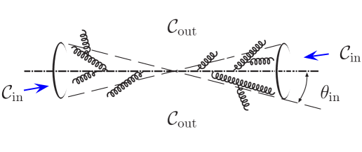
Figure 12: Two jet event in $e^{+}e^{-}$ with prescribed geometry and soft emission into the region away from the jets. ${\cal C}_{\text{in}}$ and ${\cal C}_{\text{out}}$ denote the regions inside and outside the jets which for intuitiveness are characterized by an opening angle $\theta_{\text{in}}$.

Typical soft- and collinear-safe jet observables are for example broadening $B$ or thrust $T$, both defined as sums over kinematic variables of measured hadrons. To be explicit, $B=\sum_{h}\frac{|(p_{t})_{h}|}{Q}$, $1-T=\sum_{h}\frac{|(p_{t})_{h}|e^{-|\eta_{h}|}}{Q}$ where $(p_{t})_{h}$ and $\eta_{h}$ are (three dim.) hadron transverse momentum and rapidity w.r.t. the jet axis. Setting $V=B$ or $1-T$ the corresponding jet shape distributions are then defined as

$$\Sigma(Q,V)=\sum\limits_{n}\int\frac{d\sigma_{n}(Q)}{\sigma_{T}(Q)}\theta(V-\sum\limits_{h}v_{h})$$ (150)

where $d\sigma_{n}(Q)$ is the $n$-hadron distribution, $\sigma_{T}(Q)$ the total cross section and $v_{h}$ is a single hadrons contribution to the observable. The most important perturbative contributions to such variables are enhanced by soft and collinear phase space logarithms, a single emission carries at most both of them.

Thrust and broadening belong to a large class of observables in which these enhanced contributions exponentiate [78] to give a systematic perturbative expansion for the exponent of the form

$$\ln\Sigma(Q,V)=\sum\limits_{n=1}^{\infty}\alpha_{s}(Q^{2})^{n}\left(A_{n}\ln^{n+1}V+B_{n}\ln^{n}V+\ldots\right)\ .$$ (151)

The $A_{n}$ series is referred to as double logarithmic and $B_{n}$ as single logarithmic, the remaining contributions are not logarithmically enhanced. The variables considered up to this point are referred to as global: all final state hadrons are counted in the sums $\sum_{h}v_{h}$, no matter where they end up in relation to the physical jet. Non-global observables are more restrictive, they measure for instance contribution only from hadrons that end up in the region away from the physical jet. To prepare for such a measurement one distinguishes the region containing the jets (${\cal C}_{\text{in}}$) from the region safely away from the jets (${\cal C}_{\text{out}}$) as indicated in Fig. 12. To provide a prototypical example, consider the “inter jet energy flow” defined by

$$\Sigma_{e^{+}e^{-}}(Q,E_{\text{out}})=\sum_{n}\int\frac{d\sigma_{n}(Q)}{\sigma_{T}(Q)}\cdot\Theta\!\left(E_{\text{out}}-\sum_{h\,\in\,C_{\text{out}}}\omega_{h}\right)\ .$$ (152)

Here $v_{h}=\omega_{h}$ is the energy of the measured hadron and the sum is restricted to ${\cal C}_{\text{out}}$. No event with more than a total energy $E_{\text{out}}$ outside the jets is counted. In a perturbative calculation, the phase space in energy extends up to $E\sim Q/2$ which will give rise to large logarithms in $(Q/2)/E_{\text{out}}\sim E/E_{\text{out}}$, but there will be no collinear contribution since the measured particles are emitted at large angles (from the jet as a source). This implies that in the representation (151) only the single logarithmic terms contribute. While this is an important difference with the earlier global examples, it is not immediately evident, why this observable should bear any similarities with the dipole cross sections of the CGC. The careful analysis of Dasgupta and Salam [76, 77] has uncovered that in distinction to the global case these single logarithmic contributions are sensitive to the internal structure of the jet. To the required accuracy the measured soft particles can not be treated as if emitted by the initial hard $q\bar{q}$ pair. Through emission from secondary “hard” particles, the observable becomes sensitive to the internal structure of the jet. To retain this information one must keep track of the nonlinear multiple emission structure inside the jets. Nevertheless, the connection with BK and JIMWLK evolution was not apparent until a beautiful paper by Banfi, Marchesini, and Smye (BMS) [72] reformulated the numerical approach of [76, 77] (in the large $N_{c}$ limit) for exactly the observable described above in the form of an evolution equation. The equation itself is nonlinear in the part describing contributions arising inside the jet regions and linear outside. The contributions inside, quite surprisingly for most experts, have a striking analogy with the BK equation. For small angle emission in a certain frame, the analogy becomes even more striking: the contributions of BMS inside the jet regions become identical to the BK equation. That such an analogy is restricted to the in-region, is clear: in the derivation of the BK equation one assumes, in fact requires, the presence of non-linear effects everywhere and any geometric exclusiveness of the type imposed by jets was simply never considered. What appeared to be more surprising is the relation of jet physics to BFKL dynamics, which dominates the BK equation in the small density limit. This link has been established in [79] and indeed comes into play in the limit of small angle emission in a judiciously chosen frame.

Subsequently in [54], I have shown that the analogy goes further: there exists a functional evolution equation that generalizes the BMS equation to finite $N_{c}$ which parallels the JIMWLK equation. This should be not too surprising, as BK emerges from JIMWLK by means of a factorization assumption at least strongly linked with the large $N_{c}$ limit. There are useful lessons to be learned for small ${x_{\text{bj}}}$ physics from both the structure and the derivation of this new jet evolution equation. The structure teaches us about possible consequences of exclusive constraints on observables. It shows, for instance, how non-emission requirements lead to Sudakov like resummations in the restricted areas –there only the first of the resummations into eikonal factors is at work–, whereas the unrestricted areas remain subject to nonlinear evolution and experience both types of nonlinearities. The derivation was built on earlier results on amplitudes [80, 81] and thus gives direct access to them. This should provide greater technical flexibility for any generalizations that might turn out to be desirable also on the small ${x_{\text{bj}}}$ side. Not least has the presentation in the introduction been heavily influenced by the results derived in this context.

5.1 The analogy of BMS and BK equations

To present the analogy, let me give a short account of the BMS equation before I compare with the BK equation. I will closely follow the exposition in [72]. The observable considered by BMS has been given already in (152). The process is dominated by iterative soft emission from eikonalized gluons that are not deflected from their original trajectory. The natural kinematic variables are thus the directions of the emitters ($a,b,k,p,\bar{p}$ in what follows) and the corresponding energies. Phase space integrals will be written in terms of solid angles and energies.

A Mellin transformation represents the cross section in terms of transition probabilities $G_{ab}(E,E_{\text{out}})$

$$\Sigma_{e^{+}e^{-}}(E,E_{\text{out}})\>=\>\int\frac{d\nu\,e^{\nu E_{\text{out}}}}{2\pi i\nu}\>G_{p\bar{p}}(E,\nu^{-1})\simeq G_{p\bar{p}}(E,E_{\text{out}})\>,$$ (153)

where $p$ and $\bar{p}$ are the directions of the original $q$ and $\bar{q}$ respectively and a saddle point approximation has been taken.

$G_{ab}(E,E_{\text{out}})$, or $G_{ab}(E)$ for short where the explicit $E_{\text{out}}$ dependence is not needed, satisfies the BMS equation

$$\begin{split}E\partial_{E}\>G_{ab}(E)=\int\frac{d^{2}\Omega_{k}}{4\pi}\,\bar{\alpha}_{s}w_{ab}(k)\left[u(k)\,G_{ak}(E)\cdot G_{kb}(E)-G_{ab}(E)\right]\ ,\end{split}$$ (154)

where $\bar{\alpha}_{s}:=\alpha_{s}N_{c}/\pi$ and

$$w_{ab}(k)=\frac{(p_{a}p_{b})}{(p_{a}k)(kp_{b})}=\frac{1-\cos\theta_{ab}}{(1-\cos\theta_{ak})(1-\cos\theta_{kb})}$$ (155)

is the soft emission kernel. Conventions are adapted to lightlike momenta and the energies, $\omega_{p},\omega_{q}$ have been factored out in $(pq)$ compared to the 4-vector product: $p.q=\omega_{p}\omega_{q}(pq)=\omega_{p}\omega_{q}(1-\cos\theta_{pq})$.

The jet geometry is encoded in the definition of $u(k)$, which emerges from a Mellin factorization of the energy constraint in Eq. (152):

$$\Theta\Big{(}\!E_{\text{out}}\!-\!\sum_{i\in{\cal C}_{\text{out}}}\omega_{i}\!\Big{)}=\int\frac{d\nu\,e^{\nu E_{\text{out}}}}{2\pi i\nu}\,\prod_{i}u(k_{i})\>,\quad u(k)=\Theta_{\text{in}}(k)+e^{-\nu\omega}\Theta_{\text{out}}(k)\>,$$ (156)

with the $\Theta_{\text{in}}$ and $\Theta_{\text{out}}$ having support inside and outside the jet regions respectively.

The strategy employed by BMS in the derivation of Eq. (154) is surprisingly straightforward. The evolution equation was derived from the knowledge of the structure of the real emission part alone. Virtual corrections were reintroduced using the requirement of real-virtual cancellation in the infrared.

The real emission part of $G$ needed for this argument can be written as

$$G_{p\bar{p}}^{({\text{real}})}(E,E_{\text{out}})=1\!+\!\sum_{n=1}^{\infty}\!\int\prod_{i=1}^{n}\left\{\bar{\alpha}_{s}\frac{d\omega_{i}}{\omega_{i}}\frac{d^{2}\Omega_{i}}{4\pi}u(k_{i})\,\Theta(E\!-\!\omega_{i})\!\right\}W_{n}(pk_{1}\ldots k_{n}\bar{p})$$ (157)

where the phase space of soft gluons is cut by $E$. $W_{n}$ is the large $N_{c}$ factorized version of the transition probability of a hard $q\bar{q}$ color singlet into $(q\bar{q})_{\text{hard}}g^{n}_{\text{soft}}$,

$$W_{n}(pk_{1}\ldots k_{n}\bar{p})\>=\>\frac{(p\bar{p})}{(pk_{1})(k_{1}k_{2})\ldots(k_{n}\bar{p})}\>\ .$$ (158)

The line of argument then starts by taking a logarithmic derivative $E\partial_{E}$ of Eq. (157) which uniquely fixes the quadratic term in Eq. (154). This term describes the creation of a real gluon in the final state with its energy at the phase space boundary $E$. This term is affected by the jet-geometry as signalled by the factor $u(k)$. The virtual corrections are then taken into account by subtraction of a linear term (no real gluon in the final state, virtual corrections only renormalize the existing part components of the wave function) with a coefficient that ensures infrared finiteness through real virtual cancellation. Virtual corrections occur globally, both inside and outside the jet region, thus the factor $u(k)$ is absent. This yields the second term in Eq. (154).

That this indeed ensures infrared finiteness is best understood after rewriting (154) in the form

$$\begin{split}E\partial_{E}\>G_{ab}(E)&=-E\partial_{E}\>R_{ab}^{(0)}(E)\cdot G_{ab}(E)\\ &+\int\frac{d^{2}\Omega_{k}}{4\pi}\,\bar{\alpha}_{s}w_{ab}(k)\,u(k)\,\left[\,G_{ak}(E)\cdot G_{kb}(E)-G_{ab}(E)\,\right]\ .\end{split}$$ (159)

where $R_{ab}^{(0)}(E)$ is called the single log Sudakov radiator for bremsstrahlung emission

$$R_{ab}^{(0)}(E)\>=\>\int_{0}^{E}\frac{d\omega}{\omega}\int\frac{d^{2}\Omega_{k}}{4\pi}\,\bar{\alpha}_{s}\,w_{ab}(k)\,[1-u(k)]\>=\>\Delta\cdot r_{ab}\>,$$ (160)

BMS show that to good accuracy one may take $u(k)$ to restrict the phase space integrals to the outside region for the Sudakov radiator term and to the inside region for the remainder of Eq. (159).

With integration in the Sudakov term restricted to the out region, one recognizes that there is no danger of encountering any ill effects from the poles of the kernel in this term. For the other term one needs to prove (see [72]) that $G_{aa}(E)=1$. Then the quadratic and the linear terms cancel where the kernels diverge, rendering the expression finite.

For more details on the ingredients as well as the physics of this equation see [72, 76, 77, 80, 81] and references therein.

It is now straightforward to compare the BMS equation, Eq. (154), to the BK equation in its incarnation in terms of $S_{Y;\bm{xy}}$:

$$\partial_{Y}S_{Y;\bm{xy}}=\frac{\alpha_{s}N_{c}}{2\pi^{2}}\int d^{2}z\ \tilde{\cal K}_{\bm{x}\bm{z}\bm{y}}\,(S_{Y;\bm{xz}}S_{Y;\bm{zy}}-S_{Y;\bm{xy}})\ .$$ (161)

Ignoring for the moment the Sudakov radiator term in Eq. (159), or setting $u(k)\to 1$ for the time being, the similarity of Eqns. (159) and (161) is striking. A one to one relationship of structures emerges if one maps directions onto transverse coordinates, the kernels onto each other and tries to view $G_{ab}(E)$ as the average of some ${\rm tr}(U^{\dagger}_{a}U_{b})/N_{c}$ (where $a$ and $b$ represent the directions of the leading hard particles):

$$G_{ab}(E)\ \overset{{\text{\normalsize?}}}{\longleftrightarrow}\ \langle{\rm tr}(U^{\dagger}_{a}U_{b})/N_{c}\rangle_{E}\ .$$ (162)

Note that this is fully compatible with the requirement that $G_{aa}(E)=1$, needed to ensure real virtual cancellation in the second term of Eq. (159). While this appears to be quite intuitive and fully in line with the physical interpretation, it is not immediately clear how precisely to perform that latter part of the translation. One would ask, for instance, how in detail to arrive at a consistent definition of these $U$s and the averaging process suggested by Eq. (162) in the light of the tree like branching process underlying the physics of the BMS equation. Additional questions would be how to reconcile their role in probabilities with that in amplitudes and many more in the same vein.

That the interpretation proposed in Eq. (162) should be possible suggests itself even more strongly, if one uses the observation made by BMS that in the small-angle-emission limit in a carefully chosen frame where the measure turns flat and the kernels agree completely:

$$w_{ab}(k)\to\tilde{\cal K}_{{\hat{a}}{\hat{k}}{\hat{b}}}\ .$$ (163)

This is the region where Marchesini and Mueller [79] have established the link between jet and BFKL-dynamics.

5.2 From JIMWLK to BK: generalizing BMS by analogy

To understand what the corresponding nonfactorized equation might look like, recall the chain of argument leading from the JIMWLK equation Eq. (81) via Eq. (3.2) to the pre-factorized from of the BK equation (94). From this short calculation it is pretty obvious that the linear and nonlinear terms arise in essence from the first and second term in Eq.(88):

$$H_{\text{JIMWLK}}= -\frac{1}{2}\frac{\alpha_{s}}{\pi^{2}}\ {\cal K}_{\bm{xzy}}\ \big{[}i\nabla^{a}_{\bm{x}}i\nabla^{a}_{\bm{y}}+i\bar{\nabla}^{a}_{\bm{x}}i\bar{\nabla}^{a}_{\bm{y}}+\tilde{U}_{\bm{z}}^{ab}(i\bar{\nabla}^{a}_{\bm{x}}i\nabla^{b}_{\bm{y}}+i\nabla^{a}_{\bm{x}}i\bar{\nabla}^{b}_{\bm{y}})\big{]}\ .$$

Note that this is in line with the interpretation of these terms as virtual and real contributions respectively. To arrive at different coefficients in linear and nonlinear terms as in Eq.(154) one simply has to allow for different Kernels respectively.

To write down the desired Fokker-Planck Hamiltonian in the jet case, one needs

1. to use the correspondences of variables and kernels noted in the above. In this step it proves useful, if I slightly redefine the functional aspect of the invariant vector fields to produce $\delta$ functions adapted to the structure imposed by the solid angle measure. To this end I will write

   $$i\nabla^{a}_{p}U_{p}=t^{a}U_{p}\bar{\delta}(p-q)$$ (164)

   where $\bar{\delta}(p-q)$ contains Jacobian factors such that

   $$\int\frac{d\Omega_{k}}{4\pi}\bar{\delta}(p-q)f(q)=f(p)\ .$$ (165)

   This will simplify expressions considerably.

2. The different coefficient in real and virtual parts are implemented by allowing for different integration kernels ${\cal K}^{(i)}$ $i=1,2$ for the two terms. Clearly both analogues of ${\cal K}^{(i)}$ will be proportional to $w_{pq}(k)$ with the proportionality factor $f^{(i)}(k)$ carrying the jet geometry via some $u(k)$ dependence.

The result of this exercise is a Fokker-Planck Hamiltonian that has been dubbed $H_{\text{ng}}$ (for “non-global”) in[54], here I refer to it generically by $H_{\text{jet}}$. I will present it in two forms, to parallel the two versions of the BMS equation, (154) and (159). To this end I will introduce an additional function $\tilde{f}^{(2)}(k)$ that will serve as the coefficient of the generalization of the Sudakov radiator term. One has the following forms of the Hamiltonian:

$$H_{\text{jet}}:= -\frac{\alpha_{s}}{2\pi}\ w_{uv}(k)\Big{[}f^{(1)}(k)\big{(}i\nabla^{a}_{{\bm{u}}}i\nabla^{a}_{{\bm{v}}}+i\bar{\nabla}^{a}_{{\bm{u}}}i\bar{\nabla}^{a}_{{\bm{v}}}\big{)}+f^{(2)}(k)\big{[}U_{\bm{k}}\big{]}^{ab}\big{(}i\bar{\nabla}^{a}_{{\bm{u}}}i\nabla^{b}_{{\bm{v}}}+i\bar{\nabla}^{a}_{{\bm{v}}}i\nabla^{b}_{{\bm{u}}}\big{)}\Big{]}$$ (166a)

in analogy with (154), and

$$H_{\text{jet}}:= -\frac{\alpha_{s}}{2\pi}\ w_{uv}(k)\Big{[}\tilde{f}^{(1)}(k)\Big{(}i\nabla^{a}_{{\bm{u}}}i\nabla^{a}_{{\bm{v}}}+i\bar{\nabla}^{a}_{{\bm{u}}}i\bar{\nabla}^{a}_{{\bm{v}}}\Big{)}$$

$$+f^{(2)}(k)\Big{(}i\nabla^{a}_{{\bm{u}}}i\nabla^{a}_{{\bm{v}}}+i\bar{\nabla}^{a}_{{\bm{u}}}i\bar{\nabla}^{a}_{{\bm{v}}}+\big{[}U_{\bm{k}}\big{]}^{ab}(i\bar{\nabla}^{a}_{{\bm{u}}}i\nabla^{b}_{{\bm{v}}}+i\bar{\nabla}^{a}_{{\bm{v}}}i\nabla^{b}_{{\bm{u}}})\Big{)}\Big{]}$$ (166b)

to parallel (159). In both cases $u,v$ and $k$ are integrated over according to an “integration convention” that uses $\frac{d\Omega_{p}}{4\pi}$ as its measure for any of the momenta. Retracing the steps leading from the definition of the JIMWLK equation to (94) by eye should make it obvious that indeed, the separation of terms in Eq. (166) is such that the first line generates the Sudakov radiator and the second the nonlinear evolution inside the jet cones.

A comparison of the result with BMS allows one to determine only the leading $N_{c}$ part of the $f^{(i)}$. Already the $1/N_{c}$ corrections are not controlled by the matching. To this accuracy the $f$ are $N_{c}$ independent:

$$f^{(2)}(k)= u(k)$$ (167a)

$$f^{(1)}(k)= 1$$ (167b)

$$\tilde{f}^{(1)}(k)= (1-u(k))\ .$$ (167c)

Eqns. (166), (167) together with a Fokker-Planck equation of the form

$$E\partial_{E}\hat{Z}_{E}[U]=-H_{\text{jet}}\hat{Z}_{E}[U]$$ (168)

define the finite $N_{c}$ generalization of the BMS equation given in[54]. One might argue that this has to be the correct result on naturalness reasons –any $N_{c}$ dependence in these equations would make it virtually impossible that they should be able to incorporate all $N_{c}$ corrections in a consistent manner– but an explicit construction of this equation from the amplitude level is much more instructive and will be reproduced below.

The most important feature of this equation is its infrared finiteness which directly relates to the real virtual cancellations being correctly encoded in Eq. (166). Considering the Sudakov term in $H_{\text{jet}}$ one finds that just as in the BMS limit, the phase space integration over $k$ is restricted to the outside region where no hard particles are to be found. Therefore there is no divergence from the poles in $w_{uv}(k)$. The second term may be recast in analogy to Eq. (82) and the same finiteness argument used there clearly carries over to this situation. By looking at the BMS limit one sees that this same cancellation of terms corresponds to a real-virtual cancellation in the conventional sense. On the functional side, real and virtual contributions arise from different terms. Contributions with an additional factor $\tilde{U}_{k}$ correspond to real emission, the rest to virtual corrections.

The idea to interpret jet transition probabilities as correlators of path-ordered exponentials in singlet projections properly takes into account gauge invariance, just the same way as the formulation of the JIMWLK equation does. The equation suggested therefore would appear to consistently encode the physics it is intended to cover with a set of very strong constraints.

5.3 An equivalent Langevin description

Just as in the small ${x_{\text{bj}}}$ situation, a translation to a Langevin type description is possible. The steps are almost identical to the ones presented in Sec. 4, just slightly complicated by the added exclusiveness, the distinction into in and out regions.

Prerequisites are (termwise) positive (semi-) definiteness of the Fokker-Planck Hamiltonian in question. Only then can one introduce a bounded noise integral – if needed separately for each positive term. If the Hamiltonian can be (termwise) separated into two conjugate factors in analogy to the structure of Eq. (82), any correlation effects can be included in the Langevin equation. The noise can then be taken to be (termwise) uncorrelated.

Fortunately all of the prerequisites listed above are also met for $H_{\text{jet}}$. In order to achieve termwise factorization, I first separate off the $f^{(2)}$ terms and further treat the two contributions proportional to $\tilde{f}^{(1)}$ separately. All of these are positive due to the definition of $u(k)$:

$$u(k)=\Theta_{\text{in}}(k)+e^{-\nu\omega}\Theta_{\text{out}}(k)$$ (169)

ensures $0<u(k)<1$ and the same then for the coefficient functions in Eq. (166).

To parallel the treatment in Sec.4.1 and 4.2 one would write the Hamiltonian on the JIMWLK level as

$$H_{\text{jet}}= \frac{1}{2}i\nabla^{a}_{u}\chi^{ab}_{uv}i\nabla^{b}_{v}$$ (170)

where $u,v$ are integrated over with $\frac{d\Omega_{u}}{4\pi}\frac{d\Omega_{v}}{4\pi}$ and

$$\chi^{ab}_{uv}= \ -\int\frac{d\Omega_{k}}{4\pi}\frac{\alpha_{s}}{\pi}w_{uv}(k)\Big{[}\tilde{f}^{(1)}(k)(1+U_{u}^{\dagger}U_{v})+f^{(2)}(k)(1-U_{u}^{\dagger}U_{k})(1-U_{k}^{\dagger}U_{v})\Big{]}^{ab}\ .$$ (171)

Factorization of $\chi$ according to $\chi={\cal E}{\cal E}^{\dagger}$ is achieved by defining a three component structure representing the three separately positive terms alluded to before:

$${\cal E}_{pk}^{ab;\mu}= \sqrt{\frac{\alpha_{s}}{\pi}}\frac{p^{\mu}}{p.k}\big{\{}\sqrt{\tilde{f}^{(1)}(k)}\delta^{ab},\sqrt{\tilde{f}^{(1)}(k)}[U^{\dagger}_{p}]^{ab},\sqrt{f^{(1)}(k)}(1-U_{p}^{\dagger}U_{k})^{ab}\big{\}}\ .$$ (172)

Correspondingly one has to introduce independent white noise for all of the components,

$$\Xi_{k}^{b;\mu}=\big{\{}(\xi^{(1)})_{k}^{b;\mu},(\xi^{(1^{\prime})})_{k}^{b;\mu},(\xi^{(2)})_{k}^{b;\mu}\big{\}}\ .$$ (173)

The only thing left to cope with is the measure and the $\delta$-functions in the noise correlator, which need to be such that

$$\big{\langle}\big{(}\int\frac{\Omega_{k}}{4\pi}{\cal E}_{pk}^{ac;\mu}\Xi_{k}^{c;\mu}\big{)}\big{(}\int\frac{\Omega_{l}}{4\pi}{\cal E}_{ql}^{ad;\nu}\Xi_{l}^{d;\nu}\big{)}\big{\rangle}=\chi_{pq}^{ab}\ .$$ (174)

Now the measure is $\frac{d\cos\theta d\phi}{4\pi}$ and one needs the correlators to read

$$\langle(\Xi^{i})_{p}^{a;\mu}(\Xi^{j})_{q}^{b;\nu}\rangle=4\pi\delta(\cos\theta_{p}-\cos\theta_{q})\delta(\phi_{p}-\phi_{q})\delta^{ij}g^{\mu\nu}\ .$$ (175)

With these preparations and the identification $Y\leftrightarrow\ln E/E_{\text{out}}$one has a Langevin equation that reads

$$\partial_{Y}\,[U_{Y;p}]_{ij}=[U_{Y;p}it^{a}]_{ij}\Big{[}\int\!\frac{d\Omega_{k}}{4\pi}\,{\cal E}_{pk}^{ab;\mu}[U_{Y;p}]\ \Xi^{b;\mu}_{Y;k}\Big{]}\ .$$ (176)

In comparison with the JIMWLK case all sigma-terms vanish because $w_{pq}(k)$ satisfies $w_{pp}(k)=0$.

Note again that any continuum notation is deceptive. The equation to consider is really a finite difference equation and upon iteration will allow for an interpretation of subsequent, ordered soft gluon emission. To this end it is instructive to rewrite the Langevin equation in terms of functional derivatives:

$$\partial_{Y}\,[U_{Y;p}]_{ij}= [U_{Y;p}it^{a}]_{ij}\Big{[}\int\!\frac{d\Omega_{k}}{4\pi}\,{\cal E}_{pk}^{ab;\mu}[U_{Y;p}]\ \Xi^{b;\mu}_{Y;k}\Big{]}$$

$$= \Big{\{}\int\!\frac{d\Omega_{q}}{4\pi}\frac{d\Omega_{k}}{4\pi}\ i{\cal E}_{pq}^{ab;\mu}[U_{Y;p}]\ \Xi^{b;\mu}_{Y;k}i\nabla^{a}_{U_{Y;q}}\Big{\}}[U_{Y;p}]_{ij}\ .$$ (177)

The operator in the last version contains two terms in its third component, the component responsible for the in-region. Using a somewhat more compact notation for the $Y$ dependence they read:

$$\int\!\frac{d\Omega_{q}}{4\pi}\int\!\frac{d\Omega_{k}}{4\pi}\,\Big{[}i({\cal E}^{3})_{pq}^{ab;\mu}\ \Xi^{b;\mu}_{k}i\nabla^{a}_{q}\Big{]}_{Y^{\prime}}=\int\!\frac{d\Omega_{q}}{4\pi}\frac{d\Omega_{k}}{4\pi}\,i\sqrt{\frac{\alpha_{s}}{\pi}}\frac{p^{\mu}}{p.q}\Big{[}(i\nabla^{a}_{p}+\tilde{U}^{ba}_{q}i\bar{\nabla}^{b}_{p})\ \Xi^{a;\mu}_{k}\Big{]}_{Y^{\prime}}\ .$$ (178)

Taking into account the fact that the Langevin description is defined only in a $Y$-discretized sense, one might be tempted to conclude that the terms containing factors $\tilde{U}_{q}$ correspond to real gluon emission, while the others would generate virtual corrections, not only in this, but also the other components.

A formal solution to (176) is

$$U_{Y,p}={\sf P}_{Y}\exp\Big{\{}i\int^{Y}_{Y_{0}}dY^{\prime}\int\!\frac{d\Omega_{q}}{4\pi}\frac{d\Omega_{k}}{4\pi}\,\Big{[}{\cal E}_{pq}^{ab;\mu}\ \Xi^{b;\mu}_{k}i\nabla^{a}_{q}\Big{]}_{Y^{\prime}}\Big{\}}U_{Y_{0},p}\ ,$$ (179)

which again is to be interpreted in a discrete sense. To write this expression I have also adapted the definition of the functional derivatives to include a $\delta$-function in $Y$: $i\nabla^{a}_{Y,p}U_{Y^{\prime}q}=-U_{Y,p}t^{a}\tilde{\delta}(p-q)\delta(Y-Y^{\prime})$.

The operator

$${\sf P}_{Y}\exp\Big{\{}i\int^{Y}_{Y_{0}}dY^{\prime}\int\!\frac{d\Omega_{q}}{4\pi}\frac{d\Omega_{k}}{4\pi}\,\Big{[}{\cal E}_{pq}^{ab;\mu}\ \Xi^{b;\mu}_{k}i\nabla^{a}_{q}\Big{]}_{Y^{\prime}}\Big{\}}$$ (180)

is the analog of the JIMWLK shower operator (149) and is not only relevant to the Langevin formulation itself. It implements subsequent real emission with virtual corrections correctly taken into account. This idea will be substantiated below in a three step process: The first step consists of explicitly constructing the real emission part of these amplitudes and comparing it to known results [80, 81]. The second step is the use of this information to recover the evolution equation (168) –this step reinstates the virtual corrections– and the third step is the equivalence of Fokker-Planck and Langevin treatment which closes the line of argument.

5.4 Amplitudes in the strongly ordered domain

In order to find a suitable starting point to derive results beyond the large $N_{c}$ limit, one has to go rather far back and start with a general discussion of soft gluon amplitudes along the lines given already in [80, 81].

To help organize the argument, I will start with the definition of a generating functional for the (tree level) amplitudes of (real) soft gluon emission from a $q\bar{q}$ pair in the strongly ordered region as already done in [54]

$$\omega_{k_{n}}\ll\omega_{k_{n-1}}\ll\ldots\omega_{k_{1}}\ll\omega_{p}<\omega_{q}$$ (181)

written as

$${\sf A}_{p\,q}^{ij}[\Xi]:=\sum\limits_{n=0}^{\infty} \int\frac{d\Omega_{k_{1}}}{4\pi}\ldots\frac{d\Omega_{k_{n}}}{4\pi}A(_{qpk_{1}\ldots k_{n}}^{ija_{1}\ldots a_{n}})i\Xi_{k_{1}}^{a_{1}}\ldots i\Xi_{k_{n}}^{a_{n}}\ .$$ (182)

The amplitudes for $n$-gluon emission from a initial $q\bar{q}$ pair are denoted by $A(_{qpk_{1}\ldots k_{n}}^{ija_{1}\ldots a_{n}})$, where the momenta $q,p,k_{1}\ldots k_{n}$ and color indices $i,j,a_{1}\ldots a_{n}$ are explicitly listed, a corresponding set of Lorentz-indices $\mu_{1}\ldots\mu_{n}$ is suppressed. (For diagrammatic representations, see Eq. (184).) They are isolated by $n$-fold (functional) differentiation w.r.t. $i\Xi$ at $\Xi=0$. At this stage, $\Xi$ is just an external source, the relationship to the noise of the Langevin description will become clear shortly.

The $A(_{qpk_{1}\ldots k_{n}}^{ija_{1}\ldots a_{n}})$ are known to satisfy an iterative structure in which the ${\text{color singlet}}\to q\bar{q}g^{n+1}_{\text{soft}}$-amplitude follows by induction from the corresponding amplitude with $n$ soft gluons. As a result, the $0$-gluon term in Eq. (182) fully determines the whole functional, although the explicit construction of the $n$-th order expression with the tools available to date becomes more and more cumbersome with growing $n$. The rules of the game have been explicitly demonstrated in [81] and require no recourse to the $1/N_{c}$ limit.

The important observation now is that there exists [54] a relatively simple, closed operator form for this generating functional. In fact it consists of an even more general operator acting on the zeroth order “hard seed” term in the sense that this operator can be applied to any “hard seed” to generate the full soft gluon cloud accompanying it, the full shower operator already presented in Eq. (180). This will be explained in this section using the existing information on tree level amplitudes and hence the discussion leads to the real emission part of this operator as given in Eq. (198).

For this purpose, a slight generalization of the definition (182) is operationally somewhat more useful, in that it allows me to specify an explicit functional form that casts the iteration step from $q\bar{q}g^{n}_{\text{soft}}$ to $q\bar{q}g^{n+1}_{\text{soft}}$ of [81] as a simple functional operation. This operation will involve nothing more complicated than the functional differentiation rules given in Eq. (85) and a suitably defined $n=0$ term to start the process of generating the amplitudes. The starting point is the definition

$${\sf A}_{p\,q}^{ij}[U,\Xi]:=\sum\limits_{n=0}^{\infty} \int\frac{d\Omega_{k_{1}}}{4\pi}\ldots\frac{d\Omega_{k_{n}}}{4\pi}A(_{qpk_{1}\ldots k_{n}}^{\tilde{i}\tilde{j}a_{1}\ldots a_{n}})\tilde{U}_{k_{1}}^{a_{1}b_{1}}i\Xi_{k_{1}}^{b_{1}}\ldots\tilde{U}_{k_{n}}^{a_{n}b_{n}}i\Xi_{k_{n}}^{b_{n}}\ [U^{\dagger}_{p}]_{i\tilde{i}}[U_{q}]_{\tilde{j}j}\ .$$ (183)

Here I have simply added a factor of $U$ in the appropriate representation to each leg of the diagrams contained in the definition of the ordered amplitudes. Diagrammatically the first few contributions read:

$${\sf A}_{p\,q}^{ij}[U,\Xi]=\begin{minipage}[c]{42.67912pt} \begin{center} \includegraphics[height=51.21504pt]{bareqqb-U} \end{center} \end{minipage}+\begin{minipage}[c]{56.9055pt} \begin{center} \includegraphics[height=51.21504pt]{qqb-gu-UXi-i} \end{center} \end{minipage}+\begin{minipage}[c]{56.9055pt} \begin{center} \includegraphics[height=51.21504pt]{qqb-gd-UXi-i} \end{center} \end{minipage}+\begin{minipage}[c]{59.75095pt} \begin{center} \includegraphics[height=51.21504pt]{qqb-g2u-UXi-i} \end{center} \end{minipage}+\begin{minipage}[c]{59.75095pt} \begin{center} \includegraphics[height=51.21504pt]{qqbggsplitu-UXi-i} \end{center} \end{minipage}+\ldots$$ (184)

Obviously Eq. (182) is just the special case at $U=1$: ${\sf A}_{p\,q}^{ij}[\Xi]={\sf A}_{p\,q}^{ij}[1,\Xi]$. The rationale behind this definition lies in the very nature of soft gluon emission underlying the construction of the amplitudes. Per definition, soft gluon emission does not change the direction of the parent (the emitter). In that role as a parent the entity (be it a quark or a gluon) is therefore written as a path ordered exponential along the direction of some momentum. Emission of a softer gluon, that in later steps will also serve as a parent will then necessarily add an adjoint factor $\tilde{U}_{k}$ and an eikonal emission vertex $J_{lk}^{\mu}t^{a}$ (with $J^{\mu}_{pk}:=\frac{p^{\mu}}{p.k}$), where the generator is to be taken in the representation of the emitting object. As all these objects are encoded as eikonal lines $U$, this will automatically occur if one writes it via invariant vector fields $i{\bar{\nabla}}^{a}_{l}$ just as in the rewrite of the Langevin equation at the end of Sec. 5.3. In functional form, one ends up with the single emission operator

$$i\int\!\frac{d\Omega_{l}}{4\pi}\frac{d\Omega_{k}}{4\pi}\,g\,J_{lk}^{\mu}\tilde{U}^{ab}_{k}\ \Xi^{b;\mu}_{k}i{\bar{\nabla}}^{a}_{l}\ .$$ (185)

Note how closely this resembles the real emission part of the Langevin equation (176). Eq. (183) should then be completely determined by the $n=0$ term in the sum which describes a $q\bar{q}$-pair without additional soft gluons: higher orders should just follow from repeated application of (185). This needs now to be checked against what is known about the soft gluon amplitudes.

First one needs to give an initial condition for this iteration, the bare $q\bar{q}$ term. This reads

$$[{\sf A}^{(0)}]_{p\,q}^{ij}[U,\Xi]=\begin{minipage}[c]{56.9055pt} \begin{center} \includegraphics[height=51.21504pt]{bareqqb-U} \end{center} \end{minipage}:=M_{2}(q,p)[U^{\dagger}_{p}U_{q}]_{ij}$$ (186)

and corresponds to a zero order amplitude of the form $A(_{qp}^{ij})=M_{2}(q,p)\delta^{ij}$.

The above prescription then claims that the $q\bar{q}g_{\text{soft}}$ term is given by

$$[{\sf A}^{(1)}]_{p\,q}^{ij}[U,\Xi]=\Big{\{}i\int\!\frac{d\Omega_{l}}{4\pi}\frac{d\Omega_{k}}{4\pi}\ g\,J_{lk}^{\mu}\tilde{U}^{ab}_{k}\ \Xi^{b;\mu}_{k}i{\bar{\nabla}}^{a}_{l}\Big{\}}[{\sf A}^{(0)}]_{p\,q}^{ij}[U,\Xi]\ .$$ (187)

To demonstrate once how to use the machinery, I will go through the steps explicitly. First insert $[{\sf A}^{(0)}]_{p\,q}^{ij}[U,\Xi]$ from (186). This yields

$$[{\sf A}^{(1)}]_{p\,q}^{ij}[U,\Xi]=\Big{\{}i\int\!\frac{d\Omega_{l}}{4\pi}\frac{d\Omega_{k}}{4\pi}\ g\,J_{lk}^{\mu}\tilde{U}^{ab}_{k}\ \Xi^{b;\mu}_{k}i{\bar{\nabla}}^{a}_{l}\Big{\}}M_{2}(q,p)[U^{\dagger}_{p}U_{q}]_{ij}\ .$$ (188)

All that is left to do is to use the differentiation rules (85) (with the adaptation to phase space (164) taken into account) and differentiate the two factors $U^{\dagger}_{p}$ and $U_{q}$. The variation eliminates the $l$ integral and one is left with

$$[{\sf A}^{(1)}]_{p\,q}^{ij}[U,\Xi]= \begin{minipage}[c]{71.13188pt} \begin{center} \includegraphics[height=51.21504pt]{qqb-gu-UXi-i} \end{center} \end{minipage}+\begin{minipage}[c]{71.13188pt} \begin{center} \includegraphics[height=51.21504pt]{qqb-gd-UXi-i} \end{center} \end{minipage}$$

$$=\int\!\frac{d\Omega_{k}}{4\pi}M_{2}(p,q)A_{pq}^{\mu}(k)[U^{\dagger}_{p}t^{a}U_{q}]_{ij}U^{ab}_{k}i\Xi^{b;\mu}_{k}=\begin{minipage}[c]{71.13188pt} \begin{center} \includegraphics[height=51.21504pt]{qqbg-U} \end{center} \end{minipage}i\Xi_{k}$$ (189)

where

$$A_{pq}^{\mu}(k)=J^{\mu}_{pk}-J^{\mu}_{qk}\ .$$ (190)

Now one isolates the amplitude via a variation in $\Xi$ and reads off

$$A(_{pqk}^{ija})=M_{2}(p,q)A_{pq}^{\mu}(k)[t^{a}]_{ij}=:M_{3}(p,k,q)[t^{a}]_{ij}$$ (191)

with $M_{3}(q,k,p)$ again as in the notation of [80, 81]. Eq. (191) in fact is identical to Eq. (40) of [81] and an additional gluon emission, i.e. iteration with Eq. (185), leads to Eq. (42) of [81] for the amplitude with $2$ soft gluons:

$$[{\sf A}^{(2)}]_{p\,q}^{ij}[U,\Xi]= \begin{minipage}[c]{71.13188pt} \begin{center} \includegraphics[height=51.21504pt]{qqb-g2u-UXi-i} \end{center} \end{minipage}+\begin{minipage}[c]{71.13188pt} \begin{center} \includegraphics[height=51.21504pt]{qqb-gu-gd-UXi-i} \end{center} \end{minipage}+\begin{minipage}[c]{71.13188pt} \begin{center} \includegraphics[height=51.21504pt]{qqbggsplitu-UXi-i} \end{center} \end{minipage}$$

$$+\begin{minipage}[c]{71.13188pt} \begin{center} \includegraphics[height=51.21504pt]{qqb-g2d-UXi-i} \end{center} \end{minipage}+\begin{minipage}[c]{71.13188pt} \begin{center} \includegraphics[height=51.21504pt]{qqb-gu-gd-UXi-i-mirr} \end{center} \end{minipage}+\begin{minipage}[c]{71.13188pt} \begin{center} \includegraphics[height=51.21504pt]{qqbggsplitd-UXi-i} \end{center} \end{minipage}\ .$$ (192)

(The color algebra for the explicit comparison is given in [54], App. A, case $n=1$.) The pattern simply follows the rules of functional differentiation and a comparison of analytic expressions for the amplitudes as given by the iteration rules of [81] was performed explicitly using symbolic algebra tools up to $n=6$, where the task starts to become time consuming. To compare beyond finite orders, a few additional tools are required.

In the above I have implemented the ordering “by hand,” simply by requesting the hierarchy (181) for the $\omega_{k_{i}}$. To write the all orders expression advertised above, I need one more ingredient: the addition of an energy integral to the emission operator (185) and an appropriate extension of the definition of $i\bar{\nabla}^{a}_{p}$ to $i\bar{\nabla}^{a}_{\omega_{p},p}$ defined such that

$$i\bar{\nabla}^{a}_{\omega_{p},p}U_{q}=t^{a}U_{p}\tilde{\delta}(p-q)$$ (193)

where $\tilde{\delta}(p-q)$ is adapted to the measure used in the momentum and energy integrations. The natural choice for the latter is to replace the solid angle integrations in (185) by full fledged phase space integrations:

$$\frac{d\Omega_{k}}{4\pi}\to d\Phi_{k}:=\frac{d^{4}k}{(2\pi)^{4}}\delta(k^{2})\theta(\omega_{k})=\frac{\omega_{k}d\omega_{k}}{(2\pi)^{2}}\frac{d\Omega_{k}}{4\pi}\theta(\omega_{k})\ .$$ (194)

$\tilde{\delta}(p-q)$ is then defined as the appropriate $\delta$ function on the forward light cone, i.e. with Jacobian factors such that

$$\int d\phi_{k}\tilde{\delta}(p-k)f(k)=f(p)\ .$$ (195)

(Note again the similarity of the roles played by $Y$-ordering in the Langevin description and energy ordering in this case.) With these definitions it is straightforward to verify that a replacement of the solid angle integrations in the above by phase space integrations leads to no change in the previous results, if one implements energy ordering for subsequent definitions with ordering $\theta$-functions, just as one would for the contour parameter in case of path ordered exponential. To leading logarithmic accuracy this will not change the result for the evolution equation.

By now it should appear to be the natural choice, if I write for the generating functional (again suppressing the $\omega$-label for compactness)

$${\sf A}_{p\,q}^{ij}[U,\Xi]= {\sf P}_{\omega_{k}}\exp\Big{\{}i\int\!d\Phi_{l}d\Phi_{k}\ g\,J_{lk}^{\mu}\tilde{U}^{ab}_{k}\ \Xi^{b;\mu}_{k}i{\bar{\nabla}}^{a}_{l}\Big{\}}[{\sf A}^{(0)}]_{p\,q}^{ij}[U,\Xi]\ ,$$ (196)

where ${\sf P}_{\omega_{k}}$ implements the strong ordering of Eq. (181). I should actually use a notation that displays the dependence on the functional form supplied in the zero emission part and for instance write ${\sf A}_{p\,q}^{ij}[U,\Xi,M_{2}(p,q)]$.

In analogy with path ordered exponentials, this implies that the exponential series is to be interpreted as

$${\sf P}_{\omega_{k}} \exp\Big{\{}i\int\!d\Phi_{k}d\Phi_{l}\ g\,J_{lk}^{\mu}\tilde{U}^{ab}_{k}\ \Xi^{b;\mu}_{k}i{\bar{\nabla}}^{a}_{l}\Big{\}}$$

$$:= \sum\limits_{n=0}^{\infty}{\sf P}_{\omega_{k}}\Big{[}\Big{\{}i\int\!d\Phi_{k_{n}}d\Phi_{l_{n}}\ g\,J_{l_{n}k_{n}}^{\mu_{n}}\tilde{U}^{a_{n}b_{n}}_{k_{n}}\ \Xi^{b_{n};\mu_{n}}_{k_{n}}i{\bar{\nabla}}^{a_{n}}_{l_{n}}\Big{\}}\ldots\Big{\{}i\int\!d\Phi_{k_{1}}d\Phi_{l_{1}}\ g\,J_{l_{1}k_{1}}^{\mu_{1}}\tilde{U}^{a_{1}b_{1}}_{k_{1}}\ \Xi^{b_{1};\mu_{1}}_{k_{1}}i{\bar{\nabla}}^{a_{1}}_{l_{1}}\Big{\}}\Big{]}\ ,$$ (197)

where the $1/n!$ are absent due to the explicit ordering of the subsequent soft emissions. For compactness [54] let ${\sf U}[\Xi,U]$ denote the operator

$${\sf U}[\Xi,U]:={\sf P}_{\omega_{k}}\exp\Big{\{}\int\!d\Phi_{k}d\Phi_{l}\ g\,J_{lk}^{\mu}\tilde{U}^{ab}_{k}\ \Xi^{b;\mu}_{k}i{\bar{\nabla}}^{a}_{l}\Big{\}}\ .$$ (198)

The explicit mention of the $U$-field in the notation will be needed later when different types of eikonal fields appear. ${\sf U}[\Xi,U]$ has a meaning independent of the bare ($n=0$) term it is used to act on. It is called the (real) shower operator and arises wherever one is forming that ordered soft gluon cloud around a hard seed.

With these tools a direct comparison with the iterative scheme of [81] at all orders becomes possible. In essence all that is left to confirm is that the iteration in the shower operator leads to the same result as the induction step from $n$ to $n+1$ gluons in [81]. This has been done in [54].

It is already apparent that the structure contained in the above is very similar to the information contained in the Langevin equation. This has been used to derive the RG equation stated earlier [54]. The main observation in this regard is that, as a consequence of the strong ordering, any $\frac{\delta}{\delta\Xi^{a;\mu}_{k}}$ in which $k$ is at (or near) the phase space boundary, there will be only a contribution from the first emitted gluon ($n=1$). As a consequence, for such variations one gets (h.b. stands for hard boundary)

$$\frac{\delta}{\delta\Xi^{b;\mu}_{k}}\bigg{|}_{\text{h.b.}}{\sf U}[\Xi,U]={\sf U}[\Xi,U]\Big{\{}i\int\!d\Phi_{l}\ J_{lk}^{\mu}\tilde{U}^{ab}_{k}i{\bar{\nabla}}^{a}_{l}\Big{\}}\ .$$ (199)

Note that

$${\sf A}_{p\,q\,k}^{ijb}[U,\Xi,M_{3}(p,k,q)]:={\sf U}[\Xi,U]\ \tilde{U}^{ab}_{k}[U^{\dagger}_{p}t^{a}U_{q}]_{ij}M_{3}(p,k,q)$$ (200)

is the $q\bar{q}g$ counterpart to Eq. (196). In short, Eq. (199) states, that under variation at the phase space boundary, one relates the generating functional for a given tower of amplitudes to that of a tower with an additional hard gluon. For the above example it relates the amplitudes with a hard $q\bar{q}$ to those with hard $q\bar{q}g$ content:

$$\frac{\delta}{\delta i\Xi^{b;\mu}_{k}}\bigg{|}_{\text{h.b.}}{\sf A}_{p\,q}^{ij}[U,\Xi,M_{2}(p,q)]={\sf A}_{p\,q\,k}^{ijb}[U,\Xi,A_{p\,q}^{\mu}(k)M_{2}(p,q)]\ ,$$ (201)

or diagrammatically

$$\frac{\delta}{\delta i\Xi^{b;\mu}_{k}}\bigg{|}_{\text{h.b.}}\>{\sf U}[\Xi,U]\>\begin{minipage}[c]{56.9055pt} \begin{center} \includegraphics[height=51.21504pt]{bareqqb-U} \end{center} \end{minipage}=\ {\sf U}[\Xi,U]\begin{minipage}[c]{71.13188pt} \begin{center} \includegraphics[height=51.21504pt]{qqbg-U} \end{center} \end{minipage}\ .$$ (202)

These two items, the ordered nature leading to (199) under “hard” variations, and the fact that in this situation the number of hard legs of the soft emission amplitudes is increased by one, as exemplified in (202), will be the core observations behind the evolution equation I am aiming at.

5.5 Transition probabilities from $\Xi$ averages

As a first step to understand how to translate the above into expressions for transition probabilities, let me take the situation of a (real) $q\bar{q}g^{n}_{\text{soft}}$ soft emission amplitude in which one must obtain the standard result

$$A(_{qpk_{1}\ldots k_{n}}^{ija_{1}\ldots a_{n}})[A(_{qpk_{1}\ldots k_{n}}^{ija_{1}\ldots a_{n}})]^{\dagger}= \sum\limits_{\Pi_{n+2}(l)}\sum\limits_{\Pi_{n+2}(l^{\prime})}M_{n}(q,q_{l_{1}},\ldots,q_{l_{n}},p)M_{n}(q,q_{l_{1}},\ldots,q_{l_{n}},p)^{*}$$

$$\hskip 56.9055pt\times{\rm tr}(t^{a_{l_{1}}}\ldots\ldots t^{a_{l_{n}}}t^{a_{l^{\prime}_{n}}}\ldots\ldots t^{a_{l^{\prime}_{1}}})\ ,$$ (203)

with gluon momenta in the final state labelled by $q_{1},\ldots,q_{n}$. Indeed, the same expression is obtained, if one considers the $\Xi$ averaged product of functionals

$$\langle[{\sf A}^{(n)}]_{p\,q}^{ij}[U,\Xi][{\sf A}^{(n)}]_{p\,q}^{ij}[U,\Xi]^{\dagger}\rangle_{n,\Xi}$$ (204)

if the average is defined with a Gaussian distribution for $\Xi$ in which only strongly ordered modes $q_{1},\ldots,q_{n}$ have support. I write

$$\langle\ldots\rangle_{n\Xi}:=\det(M_{n})^{\frac{1}{2}}\int\!D[\Xi]\ldots e^{-\frac{1}{2}\int d\phi_{p}d\phi_{q}\Xi_{p}^{t}M^{-1}_{n,\,pq}\Xi_{q}}$$ (205)

where $d\phi_{k}$ denotes the phase space integral for momentum $k$ and I have suppressed discrete indices. $M$ defines the $\Xi$ correlator, which in the fully exclusive case considered above would read

$$M_{n,\,pq}^{a,\mu\ b,\nu}=\langle\Xi_{p}^{a,\mu}\Xi_{q}^{b,\nu}\rangle_{n,\Xi}=\delta^{ab}g^{\mu\nu}\tilde{\delta}(p-q)\ \sum\limits_{i=1}^{n}\tilde{\delta}(q-q_{i})\ .$$ (206)

In this case, because of the strong ordering of momenta in the amplitudes, the $\Xi$ integral will strictly pair off the one available momentum $k_{i}$ in the amplitudes falling into the same range as $q_{i}$ with the latter.

As such, this is only true if I have ordering in the emission vertices, either done by hand in the 2-d version, or via ${\sf P}_{\omega_{k}}$ in the 2+1-d formulation. Only then, unwanted cross terms are excluded. The $U$ factors just cancel trivially.

To make contact with the non-global observables of the BMS setting, one needs to depart from the fixed $n$ situation and replace the $\sum\limits_{i=1}^{n}\tilde{\delta}(q-q_{i})$, which selects a given set of final state momenta in the case where the number of final state gluons is specified, by a cutoff criterion that restricts real emission by geometry and energy. By writing

$$M_{pq}^{a,\mu\ b,\nu}=\langle\Xi_{p}^{a,\mu}\Xi_{q}^{b,\nu}\rangle_{\Xi}=\delta^{ab}g^{\mu\nu}\tilde{\delta}(p-q)\ \theta(E-\omega_{q})u(q)\ ,$$ (207)

one can indeed go beyond a final state with a fixed number of gluons and consider

$$\langle{\sf A}_{p\,q}^{ij}[U,\Xi]{\sf A}_{p\,q}^{ij}[U,\Xi]^{\dagger}\rangle_{\Xi}\ ,$$ (208)

which will provide the finite $N_{c}$-generalization of $G_{ab}^{(\text{real})}$ of BMS.

In fact any degree of inclusiveness may be imposed by modifying the restrictions on the allowed modes appearing on the r.h.s. of Eq. (207).

This realization should make it clear how to include virtual corrections right from the outset, by a fairly simple modification of the above. I will refrain from doing so here and instead keep a closer parallel with the strategy employed by [72, 80, 81] and use the expressions for real emission to deduce the structure of the evolution equation.

5.6 Evolution equations for soft semi-inclusive quantities

For semi-inclusive quantities like the non-global observables of [72], in which one sums over a given, limited phase space volume of soft gluons, it is natural to ask for the dependence on that phase space boundary. Unlike a direct calculation of the average in Eq. (208) this should lead to a tractable result that exhibits new structure. In fact, one recovers the generalization to the BMS equation suggested above.

To arrive at an evolution equation, I will simply take a derivative w.r.t. the phase space boundary of the emitted gluons in the semi-inclusive probability (208). This is in direct correspondence with the procedure used in BMS. Here it is essential that one includes the phase space boundary into the definition of $M$. Then the result is most transparently displayed using the following simple relationship, based on functional differentiation and Legendre transformation in the case of a Gaussian action (“free theory”):

$$\big{\langle}W[\Xi]\big{\rangle}_{\Xi}= N\int D[\Xi]\ W[\Xi]\ e^{-\frac{\Xi^{t}M^{-1}\Xi}{2}}=W[\frac{\delta}{i\,\delta{\cal J}}]e^{-\frac{{\cal J}^{t}M{\cal J}}{2}}\Big{|}_{{\cal J}=0}=e^{-\frac{\frac{\delta}{i\delta\Xi_{0}}M\frac{\delta}{i\delta\Xi_{0}}}{2}}W[\Xi_{0}]\Big{|}_{\Xi_{0}=0}$$ (209)

for any functional $W[\Xi]$. Here notation has been condensed even further, with all momenta, integration signs and measures suppressed. Legendre machinery is used for the last equality sign. The “classical field,” $\Xi_{0}=iM{\cal J}$, vanishes at ${\cal J}=0$.

The canonical example for $W[\Xi]$ here of course is

$$\big{\langle}W[\Xi]\big{\rangle}_{\Xi}\to\big{\langle}{\sf A}_{p\,q}^{ij}[U,\Xi]{\sf A}_{p\,q}^{ij}[U,\Xi]^{\dagger}\big{\rangle}_{\Xi}\ ,$$ (210)

which, by construction, is the finite $N_{c}$ generalization of $G^{(\text{real})}_{ab}$.

For this example one immediately realizes that the exponential of the second order differential operator on the right hand side will perform precisely the “sewing” implemented by the Gaussian weight in Eq. (208), as long as $M$ is diagonal in energies as in (207). In this case, the energy ordering ensures that

$$\frac{1}{2}\frac{\delta}{i\delta\Xi_{0}}M\frac{\delta}{i\delta\Xi_{0}}{\sf A}_{p\,q}^{ij}[U,\Xi_{0}]{\sf A}_{p\,q}^{ij}[U,\Xi]^{\dagger}=\Big{(}\frac{\delta}{i\delta\Xi_{0}}{\sf A}_{p\,q}^{ij}[U,\Xi_{0}]\Big{)}M\Big{(}\frac{\delta}{i\delta\Xi_{0}}{\sf A}_{p\,q}^{ij}[U,\Xi]^{\dagger}\Big{)}\ .$$ (211)

Let me now carry out the derivative with respect to the phase space boundary in analogy with the derivation of the BMS equation sketched in Sec. 5.1. With $M=M(E)$ a function of the phase space boundary, one immediately finds a general expression for the logarithmic $E$-derivative of the above expectation value that reads

$$E\partial_{E}\ \big{\langle}W[\Xi]\big{\rangle}_{\Xi}(E)=-\frac{1}{2}e^{-\frac{\frac{\delta}{i\delta\Xi_{0}}M(E)\frac{\delta}{i\delta\Xi_{0}}}{2}}\ \frac{\delta}{i\delta\Xi_{0}}E\partial_{E}M(E)\frac{\delta}{i\delta\Xi_{0}}\ W[\Xi_{0}]\Big{|}_{\Xi_{0}=0}\ .$$ (212)

The main point about this seemingly trivial exercise is its use in conjunction with what is already known about functional derivatives of the amplitudes of interest: Eqns. (199), (201). Note that $\partial_{E}M(E)$ will force the variations in the factor taken down from the exponential to be at the phase space boundary. Choosing $W[\Xi]={\sf A}_{p\,q}^{ij}[U,\Xi]{\sf A}_{p\,q}^{ij}[U,\Xi]^{\dagger}$, the square of the generating functional of $q\bar{q}\,g^{n}_{\text{soft}}$ amplitudes, this location at the boundary will lead to the appearance of the square of the generating functional of $q\bar{q}g\,g^{n}_{\text{soft}}$ on the right hand side as follows from (201), (202).

This marks an important difference compared to the BMS case at infinite $N_{c}$: the equation does not close. Instead higher and higher hard correlators will enter: Clearly, an evolution equation for the $q\bar{q}g\,g^{n}_{\text{soft}}$ amplitudes will then couple in turn to the corresponding object for $q\bar{q}g^{2}\,g^{n}_{\text{soft}}$ amplitudes and so forth. One is faced with an infinite hierarchy. All quantities encountered in this hierarchy can be defined in complete analogy to the examples presented in (196) and (200). One simply uses the desired combination of $U$-factors as the “bare” term in the tower of amplitudes one is interested in.

This implies that firstly, it is not sufficient to consider only the evolution equation for $q\bar{q}g^{n}_{\text{soft}}$ amplitudes alone. Instead one has to capture the complete infinite coupled hierarchy of equations in one. Secondly, it indicates that such a step is possible, since the objects of interest have already been identified and indeed can be written down in a general form. The evolution equations then follow from (212).

I therefore proceed to define the (tree level) generating functional based on $m$ hard particles, a general “antenna pattern,” by

$${\sf A}_{p_{1}\ldots p_{m}}^{i_{1}\ldots i_{n}}[U,\Xi]{\sf A}_{p_{1}\ldots p_{m}}^{i_{1}\ldots i_{n}}[V,\Xi]^{\dagger}={\sf U}[\Xi,U]\ (UV^{\dagger})_{p_{1}}^{(\dagger)}\otimes\ldots\otimes(UV^{\dagger})_{p_{m}}^{(\dagger)}\ {\sf U}[\Xi,V]^{\dagger}\Big{|}_{U=V}\ .$$ (213)

The factor $(UV^{\dagger})_{p_{1}}^{(\dagger)}\otimes\ldots\otimes(UV^{\dagger})_{p_{m}}^{(\dagger)}$ in this expression generalizes the expression for the bare particles of the $q\bar{q}$ case (the ${\sf A}_{p\,q}^{ij}[U,\Xi]{\sf A}_{p\,q}^{ij}[U,\Xi]^{\dagger}$ from above) from $2$ to $m$ hard legs, and the ${\sf U}[\Xi,U]\ \ldots\ {\sf U}[\Xi,V]^{\dagger}\Big{|}_{U=V}$ implement the showering. I have given only $q$ and $\bar{q}$ factors as any gluon can be written in terms of these as $\tilde{(UV^{\dagger})}_{k}^{ab}=2{\rm tr}(t^{a}(UV^{\dagger})_{k}^{\dagger}t^{b}(UV^{\dagger})_{k})$.

One can now study the evolution of the expectation value of a given object of the type (213) or directly study a generating functional for all such objects in one go. The latter is given by

$${\sf W}[j^{\dagger},j]:= \Big{\langle}{\sf U}[\Xi,U]\ e^{i2{\rm tr}j^{\dagger}UV^{\dagger}+i2{\rm tr}(UV^{\dagger})^{\dagger}j}\ {\sf U}[\Xi,V]^{\dagger}\Big{\rangle}_{\Xi}\Big{|}_{U=V}$$ (214)

with integrals in the source exponents understood. Appropriate variations with respect to $j$ and $j^{\dagger}$ at $j=0$ will then select a given tower of $\text{in}\to\text{hard}\,g^{n}_{\text{soft}}$ probabilities entering the hierarchy. Since, besides the phase space constraints contained in $M$, it is the particle content of the bare terms that define the amplitudes, a notation that emphasizes this is needed. To this end I will write

$$\frac{\delta}{i\delta j^{(\dagger)}_{p_{1}}}\ldots\frac{\delta}{i\delta j^{(\dagger)}_{p_{m}}}{\sf W}[j^{\dagger},j]= \Big{\langle}{\sf U}[\Xi,U]\ (UV^{\dagger})_{p_{1}}^{(\dagger)}\otimes\ldots\otimes(UV^{\dagger})_{p_{m}}^{(\dagger)}\ {\sf U}[\Xi,V]^{\dagger}\Big{\rangle}_{\Xi}\Big{|}_{U=V}$$

$$=: \Big{\langle}\ (UV^{\dagger})_{p_{1}}^{(\dagger)}\otimes\ldots\otimes(UV^{\dagger})_{p_{m}}^{(\dagger)}\ \Big{\rangle}_{UV^{\dagger}}^{\text{real}}$$ (215)

where the $UV^{\dagger}$ average in the second line is to be taken with a yet unknown weight that reproduces the l.h.s.. The idea is to interpret the soft gluon average as an average over $UV^{\dagger}$ configurations. This is completely legal, if somewhat formal as long as the only definition of the weight of the average is through (5.6).

Nevertheless, it is this reinterpretation that will allow to make contact with the Fokker-Planck formulation of Sec. 5.2 and that is all that is really needed.

For $m=2$ and an adapted choice for the color structure one encounters

$$\langle{\rm tr}((UV^{\dagger})^{\dagger}_{p}(UV^{\dagger})_{q})/N_{c}\rangle_{UV^{\dagger}}^{\text{real}}=:G_{ab}^{(\text{real})}(E)$$ (216)

and thus provides the precise definition of what was still a bit vague in (162). Eq. (5.6) is of course much more general than that: it defines the real emission part for a general antenna pattern, as these will all be needed for the evolution equations. Inclusion of virtual contributions will be discussed below. Note that the eikonal lines appearing in (5.6) have the interpretation of a product $UV^{\dagger}$ of contributions from both the amplitude and the conjugate amplitude.

With (209) one then has

$${\sf W}[j^{\dagger},j]= e^{-\frac{\frac{\delta}{i\delta\Xi_{0}}M(E)\frac{\delta}{i\delta\Xi_{0}}}{2}}{\sf U}[\Xi_{0},U]\ e^{i2{\rm tr}j^{\dagger}UV^{\dagger}+i2{\rm tr}(UV^{\dagger})^{\dagger}j}\ {\sf U}[\Xi_{0},V]^{\dagger}\Big{|}_{U=V}$$

$$= \big{\langle}e^{i2{\rm tr}j^{\dagger}UV^{\dagger}+i2{\rm tr}(UV^{\dagger})^{\dagger}j}\big{\rangle}_{UV^{\dagger}}^{\text{real}}\ .$$ (217)

This demonstrates that ${\sf W}[j^{\dagger},j]$ is in complete analogy with (the real emission part of) $\bar{Z}[J,J^{\dagger}]$ in the derivation of the JIMWLK equation of Sec. 3.1.

To find the evolution equation for this (meta-) functional and with it the infinite hierarchy of evolution equations alluded to above, all that is left to do, is to put together Eqns. (212), (211), and (199) to get the dependence on phase space boundaries for arbitrary $UV$-correlators (bare $m$-jet probabilities). This yields the r.h.s. for the real emission contribution:

$$e^{-\frac{\frac{\delta}{i\delta\Xi_{0}}M(E)\frac{\delta}{i\delta\Xi_{0}}}{2}}{\sf U}[\Xi_{0},U]$$

$$\Big{\{}g\,J_{lk}^{\mu}\tilde{U}^{ab}_{k}i{\bar{\nabla}}^{a}_{U_{l}}\Big{\}}[E\partial_{E}M(E)]_{ll^{\prime}\,\mu\mu^{\prime}}^{bb^{\prime}}\Big{\{}g\,J_{l^{\prime}k^{\prime}}^{\mu^{\prime}}\tilde{V}^{a^{\prime}b^{\prime}}_{k^{\prime}}i{\bar{\nabla}}^{a}_{V_{l}^{\prime}}\Big{\}}\ e^{i2{\rm tr}j^{\dagger}UV^{\dagger}+i2{\rm tr}(UV^{\dagger})^{\dagger}j}$$

$$\ {\sf U}[\Xi_{0},V]^{\dagger}\Big{|}_{U=V}\ .$$ (218)

To arrive at a meaningful answer one still has to supplement virtual corrections. They are correctly incorporated as usual, by simply subtracting the corresponding term proportional to the original transition probability. This was done in the derivation of the BMS equation and it also applies to the full hierarchy. For concreteness, and without loss of generality, I will demonstrate how to achieve this for the case of $m$ hard particles shown in Eq. (5.6).

To understand the constraints on the virtual corrections, let me first study the real emission contribution in some more detail. Omitting, for the moment, the operator that implements the soft gluon shower and the expectation value in the expression for the real emission part,

$$e^{-\frac{\frac{\delta}{i\delta\Xi_{0}}M(E)\frac{\delta}{i\delta\Xi_{0}}}{2}}{\sf U}[\Xi_{0},U]\ldots{\sf U}[\Xi_{0},V]^{\dagger}\Big{|}_{U=V}\ ,$$

one has to consider

$$\Big{\{}g\,J_{lk}^{\mu}\tilde{U}^{ab}_{k}i{\bar{\nabla}}^{a}_{U_{l}}\Big{\}}[E\partial_{E}M(E)]_{ll^{\prime}}\delta^{bb^{\prime}}g_{\mu\mu^{\prime}}\Big{\{}g\,J_{l^{\prime}k^{\prime}}^{\mu^{\prime}}\tilde{V}^{a^{\prime}b^{\prime}}_{k^{\prime}}i{\bar{\nabla}}^{a}_{V_{l}^{\prime}}\Big{\}}\ (UV^{\dagger})_{p_{1}}^{(\dagger)}\otimes\ldots\otimes(UV^{\dagger})_{p_{m}}^{(\dagger)}$$ (219)

and evaluate the variations. Inserting the BMS choice (207) for $M$, it is easy to collect all the factors and to make the $k$ integration explicit (I keep the integration convention for $l$ and $l^{\prime}$ for readability):

$$\eqref{eq:real-emission-1}= \int\frac{d\omega_{k}}{\omega_{k}}E\delta(E-\omega_{k})\frac{d\Omega_{k}}{4\pi}\frac{\alpha_{s}}{\pi}w_{ll^{\prime}}(k)(\tilde{UV}^{\dagger})^{ab}_{k}i{\bar{\nabla}}^{a}_{U_{l}}i{\bar{\nabla}}^{b}_{V_{l}^{\prime}}\ (UV^{\dagger})_{p_{1}}^{(\dagger)}\otimes\ldots\otimes(UV^{\dagger})_{p_{m}}^{(\dagger)}$$

$$= \int\!\frac{d\Omega_{k}}{4\pi}\frac{\alpha_{s}}{\pi}w_{ll^{\prime}}(k)(\tilde{UV}^{\dagger})^{ab}_{k}i{\bar{\nabla}}^{a}_{U_{l}}i{\bar{\nabla}}^{b}_{V_{l}^{\prime}}\ (UV^{\dagger})_{p_{1}}^{(\dagger)}\otimes\ldots\otimes(UV^{\dagger})_{p_{m}}^{(\dagger)}\Big{|}_{\omega_{k}=E}\ .$$ (220)

In this expression $\omega_{l}$ and $\omega_{l}^{\prime}$ will be made hard when the functional derivatives hit the $U$ and $V$. The energy part of the corresponding phase space integrals will be eliminated at the same time. In summary one will end up with 3 “hard” momenta $k,l,l^{\prime}$.

Carrying out the differentiations, a sum over pairings will emerge, with different color structures depending on whether one hits $q$ or $\bar{q}$ lines. Concentrating on the individual terms in this sum, it is obvious that one has to deal with 4 different combinations, corresponding to the pairings $qq$, $q\bar{q}$, $\bar{q}q$, and $\bar{q}\bar{q}$ completely in parallel with Eqns. (61) of the JIMWLK case.

At this point it is, however, more efficient to directly use the unifying properties of the left and right invariant vector fields without exploring these structures explicitly. This may be done by noting that Eq. (219) allows for a very elegant rewrite:

$$\text{~{}\eqref{eq:real-emission}}= \frac{\alpha_{s}}{2\pi}w_{pq}(k)u(k)(\tilde{UV^{\dagger}})^{ab}_{k}\big{(}i\bar{\nabla}_{(UV^{\dagger})_{p}}^{a}i\nabla^{b}_{(UV^{\dagger})_{q}}+i\bar{\nabla}_{(UV^{\dagger})_{q}}^{a}i\nabla^{b}_{(UV^{\dagger})_{p}}\big{)}\$$

$$\hskip 216.81pt(UV^{\dagger})_{p_{1}}^{(\dagger)}\otimes\ldots\otimes(UV^{\dagger})_{p_{m}}^{(\dagger)}\ .$$ (221)

Eq. (5.6) follows from a direct correspondence of $i\bar{\nabla}^{a}_{(UV^{\dagger})_{k}}$ with $i\bar{\nabla}^{a}_{U_{k}}$ acting on the amplitude, and $i\nabla^{a}_{(UV^{\dagger})_{k}}$ with $i\bar{\nabla}^{a}_{V_{k}}$ acting on the complex conjugate factor. In Eq. (5.6) it is possible to anticipate that the energies will all be made hard by functional differentiation on the hard factors $(UV^{\dagger})_{p_{i}}$ and thus to go back to the original definition of the variations without the energy $\delta$-function. This allows to use an integration convention that employs the solid angle integrations only and a symmetric treatment of $k,p,q$ in this equation. Reinstating the shower-operators and the expectation value, one arrives at the real emission part of the evolution equation

$$\Big{\langle}\frac{\alpha_{s}}{2\pi}w_{pq}(k)u(k)(\tilde{UV^{\dagger}})^{ab}_{k}\big{(}i\bar{\nabla}_{(UV^{\dagger})_{p}}^{a}i\nabla^{b}_{(UV^{\dagger})_{q}}+i\bar{\nabla}_{(UV^{\dagger})_{q}}^{a}i\nabla^{b}_{(UV^{\dagger})_{p}}\big{)}\$$

$$\hskip 216.81pt(UV^{\dagger})_{p_{1}}^{(\dagger)}\otimes\ldots\otimes(UV^{\dagger})_{p_{m}}^{(\dagger)}\Big{\rangle}_{UV^{\dagger}}(E)\ .$$ (222)

Virtual corrections do not depend on the physical process at hand: While the real emissions are confined to the inside regions and hence carry a factor $u(k)$, virtual corrections appear everywhere and therefore have no such factor. Moreover the factor $(\tilde{U}V^{\dagger})_{k}^{ab}$ will be replaced by $\delta^{ab}$ and the vector fields will have to act twice within either the amplitude or its complex conjugate, leading to $i\nabla_{(UV^{\dagger})_{p}}^{a}i\nabla^{a}_{(UV^{\dagger})_{q}}$ and an analogous barred contribution instead of the mixed ones in Eq. (5.6). For symmetry reasons, one therefore expects the virtual corrections to read

$$\Big{\langle}\frac{\alpha_{s}}{2\pi}w_{pq}(k)\big{(}i\nabla_{(UV^{\dagger})_{p}}^{a}i\nabla^{a}_{(UV^{\dagger})_{q}}+i\bar{\nabla}_{(UV^{\dagger})_{q}}^{a}i\bar{\nabla}^{a}_{(UV^{\dagger})_{p}}\big{)}\ (UV^{\dagger})_{p_{1}}^{(\dagger)}\otimes\ldots\otimes(UV^{\dagger})_{p_{m}}^{(\dagger)}\Big{\rangle}_{UV^{\dagger}}(E)\ ,$$ (223)

where the overall sign and normalization is fixed by real virtual cancellation: only with this choice do they add up to an infrared finite Fokker-Planck Hamiltonian, which happens to coincide with the expression conjectured in Sec. 5.1. Indeed, the operator appearing in the sum of (5.6) and (223) is nothing but $-H_{\text{jet}}$ of Eq. (166a) with the $f^{(i)}$ completely determined. In particular, there is no room for any $N_{c}$ dependence of the coefficients from this argument.

To summarize, it has been shown that

$$E\partial_{E}\ \Big{\langle}e^{i2{\rm tr}j^{\dagger}UV^{\dagger}+i2{\rm tr}(UV^{\dagger})^{\dagger}j}\Big{\rangle}_{UV^{\dagger}}(E)=-\Big{\langle}\ H_{\text{jet}}\ e^{i2{\rm tr}j^{\dagger}UV^{\dagger}+i2{\rm tr}(UV^{\dagger})^{\dagger}j}\ \Big{\rangle}_{UV^{\dagger}}(E)\ .$$ (224)

The only argument still missing is about how to reverse the step leading from (81) to (90).

This follows from the fact that the identity holds for arbitrary $j$ and $j^{\dagger}$, i.e. the fact that the above is completely independent of the type of correlator considered. The result is, as advertised in Sec. 5.2, the evolution equation

$$E\partial_{E}\ \hat{Z}_{E}[UV^{\dagger}]=-H_{\text{jet}}\ \hat{Z}_{E}[UV^{\dagger}]$$ (225)

for the weight $Z_{E}[UV^{\dagger}]$ used to define the averages $\langle\ldots\rangle_{UV^{\dagger}}(E)$. This completes the derivation of Eq. (168).

5.7 The two types of nonlinearities; $N_{c}$ and correlator factorization

Now that the interpretation of $G_{pq}(E)$ in terms of link operators suggested in (162) is understood, it seems worthwhile to recapitulate the role of the two types of nonlinearities discussed repeatedly already in the JIMWLK case: eikonalization of gluon fields into Wilson lines which enter the definitions

$$\hat{G}_{pq}:= {\rm tr}((UV^{\dagger})^{\dagger}_{p}(UV^{\dagger})_{q})/N_{c}$$ (226a)

$$G_{pq}(E):= \langle\hat{G}_{pq}\rangle_{UV^{\dagger}}(E)=\frac{1}{N_{c}}\frac{\delta}{i\delta(j_{p})_{ij}}\frac{\delta}{i\delta(j_{p})_{ij}}{\sf W}_{E}[j^{\dagger},j]\ ,$$ (226b)

as the first stage and nonlinearities in the Wilson lines themselves contained in the Fokker-Planck Hamiltonians (166) or as “second eikonalization” in the shower operators (180) as the second stage.

Jet observables provide the perfect example that the second stage is not always visible; in global observables $u(k)$ suppresses the inside contributions completely and only the outside terms survive. This completely suppresses the nonlinear terms. How this happens is again best illustrated with the evolution equation for the two point function. Starting from (225), one immediately finds

$$E \partial_{E}\langle{\rm tr}((UV^{\dagger})^{\dagger}_{p}(UV^{\dagger})_{q})/N_{c}\rangle_{UV^{\dagger}}(E)$$

$$= \int\!\frac{d\Omega_{k}}{4\pi}\frac{\alpha_{s}}{\pi}w_{pq}(k)\ \Big{\langle}u(k)\tilde{(UV^{\dagger})}_{k}^{ab}\ 2\frac{{\rm tr}(t^{a}(UV^{\dagger})_{p}t^{b}(UV^{\dagger})_{q})}{N_{c}}-2C_{\text{f}}\frac{{\rm tr}((UV^{\dagger})^{\dagger}_{p}(UV^{\dagger})_{q})}{N_{c}}\Big{\rangle}_{UV^{\dagger}}(E)\ .$$ (227)

The first term on the r.h.s., carrying the factor $u(k)$, originates from the real contribution, the second from the virtual one. By (93) this is equivalent to

$$E\partial_{E}G_{pq}(E)= \int\!\frac{d\Omega_{k}}{4\pi}\frac{\alpha_{s}}{\pi}w_{pq}(k)\Big{\langle}u(k)\big{(}\hat{G}_{pk}\hat{G}_{kq}N_{c}-\frac{\hat{G}_{pq}}{N_{c}}\big{)}-2C_{\text{f}}\hat{G}_{pq}\Big{\rangle}(E)$$ (228a)

$$= \int\!\frac{d\Omega_{k}}{4\pi}\bar{\alpha}_{s}w_{pq}(k)\Big{\langle}u(k)\big{(}\hat{G}_{pk}\hat{G}_{kq}-\hat{G}_{pq}\big{)}-\frac{2C_{\text{f}}}{N_{c}}(1-u(k))\hat{G}_{pq}\Big{\rangle}(E)\ .$$ (228b)

First and second terms contribute inside and outside the jets, the former is completely suppressed in global jet observables. In this case, all traces of the second nonlinearity are gone: since the equation is linear, nothing couples to higher n-point functions. The counterpart to the Balitsky hierarchy fully decouples. What is left is simple Sudakov exponentiation which corresponds to the fact that $G$ still corresponds to a correlator of Wilson lines.

On the other hand, this formulation has a direct link between large $N_{c}$ limit and factorization of correlators which leads to the analogue of the BK equation that triggered these explorations, the BMS equation. To see this explicitly, use (209) to represent the averaging involved in

$$G_{pq}(E)=\langle\hat{G}_{pq}\rangle_{UV^{\dagger}}(E)=\langle{\sf A}_{p\,q}^{ij}[U,\Xi]{\sf A}_{p\,q}^{ij}[U,\Xi]^{\dagger}\rangle_{\Xi}$$ (229)

and then repeat the argument of[81], Eq. (50). It is worth emphasizing that the real-virtual cancellation argument of BMS restated in Sec. 5.1 applies already to Eq. (228) itself, without any reference to the factorization argument. Infrared finiteness in the Sudakov term follows directly from the argument of BMS, while in the other term it is the definition of $\hat{G}$ that guarantees the necessary cancellations. This provides an illustration of how the more general reasoning above will lead to infrared finite results via real-virtual cancellation in any evolution equation for color singlet objects contained in the new evolution equation.

5.8 Connections with CGC physics

Here I want to discuss two types of issues concerning the relationship of the treatments of evolution in the CGC case and that of non-global jet observables. The first concerns what one can learn from the above for the interpretation of the JIMWLK equation and the extension of the underlying methods to describe new, more exclusive observables. The second type of questions concerns the treatment of jets that are created in a dense medium such as in heavy ion collisions at RHIC and the LHC.

Turning to the first of these, let me begin with the observation that the two types of terms in the JIMWLK Hamiltonian indeed have the interpretation of virtual correction and real emission terms. Any restriction on (real) soft gluon emission imposed by a choice of variables must come along with a modification of the phase space available on real emission and introduce the analogue of the factor $u(k)$ appearing in the jet case. This analogy is important with respect to a generalization away from purely central collisions in a way that remains under control perturbatively. The problem is conceptual and affects both JIMWLK and BK equations, although in the latter case the problem is easier to state. To this end, return to the discussion of IR safety of BK (and JIMWLK) evolution as illustrated with Fig. 9. IR safety was ensured by the presence of a saturation scale, which in turn emerges from the existence of a dense gluonic medium. This can confidently be expected for central collisions, but will certainly fail as soon as one starts to probe the targets periphery. In this situation the gluon density becomes small, the evolution equation reduces to the BFKL equation with all its problems of diffusion into the infrared. The culprit for this in a practical sense is the long range nature of the emission kernels ${\cal K}$ in both JIMWLK and BK. As a consequence, if one attempts to prepare an initial condition to JIMWLK or BK that has large densities only in a finite spatial range, evolution will not respect this structure – the finite size object will not stay finite but grow exponentially [82, 83] . The situation for the saturated region is more subtle [84], but that does not change the basic problem of exponential growth. Any calculation that would lead to finite range of the JIMWLK or BK kernels would necessarily have to take confinement into account, an idea somewhat at odds with the perturbative philosophy taken in this review. The same applies to attempts to phenomenologically treat the impact parameter (or $\bm{b}$) dependence of real experiments using $\bm{b}$-profiles [50, 51, 52], although the results are intriguing.

The above treatment suggests a different approach. In the jet case, space is predominantly empty, in fact the observables (be it in the non-global or global case) are designed around forbidding radiation above certain thresholds into most of space. The radiation veto then leads to Sudakov logarithms that govern the mostly empty regions, while the JIMWLK or BK nonlinearities are limited to the regions that are allowed to become dense by choice of observable. The only trace of confinement physics entering this perspective is parton hadron duality, and often nonperturbative power corrections, which can in principle be understood. All of these problems appear to be entirely separate from the evolution equations. A highly attractive alternative to the DIS-type treatment existent in the literature would thus be the definition of semi inclusive observables in the small ${x_{\text{bj}}}$ case of the type of diffractive and rapidity gap events that treat the empty regions in a manner similar to the jet case.

While this remains a task for the future, the above developments have made much of the interpretational lore that dates back to Gribov [85] to emerge transparently in the actual technical treatment. While the JIMWLK equation is an equation for the cross section, the objects entering the formal solutions of the corresponding Langevin equations, the “shower-operators” –Eq. (149) for JIMWLK and Eq. (180) for the jet case– give access to the underlying amplitudes. These amplitudes result from applying the shower operators to any type of hard “seed.” The procedure simply adds fully developed clouds of soft gluons to the hard objects used as a “seed” as exemplified by DIS at small ${x_{\text{bj}}}$, where the amplitude generated by acting on a hard $q\bar{q}$ pair may be thought of as the soft gluon part of the photon wave function. This, strictly speaking, is the justification for the description of the structure of the virtual photon wave function in Sec. 1.2. A derivation of the JIMWLK equation or an evolution equation that describes diffractive events with rapidity gaps from this perspective, based on amplitudes and with a full understanding of the operatorial content would be highly instructive.

On the other hand there are direct applications to jet measurements if the jets are created in medium. This is the generic case for jet measurements at the LHC. Let me again consider a measurement of the inter-jet energy flow (152) but with the jets created in medium as depicted in Fig. 13.

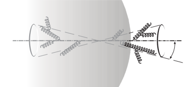
Figure 13: In medium analog of the two jet event depicted in Fig. 12. Left: Soft gluons in the inter jet region ${\cal C}_{\text{out}}$ now may be totally absorbed by the medium or be created with more energy than allowed in the out region but then softened until they fall below $E_{\text{out}}$. Right: If the medium is large enough one of the jet cones may even be completely be absorbed.

The first obvious modification is that only a subset of the soft gluons that would be measured without the medium will reach the detector, the others are absorbed by the medium. Instead of (152), the best one can hope to measure is

$$\Sigma_{e^{+}e^{-}}(Q,E_{\text{out}})=\sum_{n}\int\frac{d\sigma_{n}(Q)}{\sigma_{T}(Q)}\cdot\Theta\!\left(E_{\text{out}}-E_{\text{loss}}-\sum_{h\,\in\,C_{\text{out}}\setminus C_{\text{medium}}}\omega_{h}\right)\ .$$ (230)

where $E_{\text{loss}}$ is the net energy loss into the medium. Phase space logarithms now are of the type $\ln(E/(E_{\text{out}}-E_{\text{loss}}))$ and generically larger than in the previous case. Note that one can not lower $E_{\text{out}}$ below $E_{\text{loss}}$ once the medium is present. Also the evolution equations would change as new contributions arise. Consider for example a gluon generated inside the medium with an energy somewhat above $E_{\text{out}}$ which loses enough energy to fall below $E_{\text{out}}$ before it reaches the detector. Also this mechanism enhances the importance of the nonlinear effects. [Technically this requires a redefinition of the soft emission kernels and thus of the expressions entering (158).]

Upon considering to transplant other global jet observables like thrust or broadening from the $e^{+}e^{-}$ case to the in medium situation sketched in Fig. 13 one realizes that global sums like in (150) are not experimentally accessible as part of the contributions will be absorbed in the medium. This would appear to indicate that also other observables which are usually considered global will acquire non-global characteristics. This should lead to nonlinear evolution equations also in such cases.

The issues raised here pose interesting and important questions to be dealt with in future work – for the remainder of this review I will return to physics results from the existing evolution equations.

6 Numerical results at fixed coupling: JIMWLK and BK

6.1 Numerical results from JIMWLK simulations

While there are many numerical studies of the CGC based on the BK equation [61, 62, 63, 64, 65, 66, 67, 68, 69] there exists only one set of simulations of the full JIMWLK equation by Rummukainen and Weigert [35]. Fig. 14 shows the evolution of the dipole operator obtained there, averaged over 8 independent trajectories on a $256^{2}$ lattice, from interval $\alpha_{s}Y\equiv\alpha_{s}\ln(1/{x_{\text{bj}}})=0\ldots 2.5$. The main qualitative observation here is that the dipole operator soon approaches a specific functional scaling form, where the shape is preserved but the length scale is shortened under the evolution as discussed in Sec. 3.4. This is clearly visible on the logarithmic scale plot on the right: the Gaussian initial condition quickly settles towards the scaling solution which evolves by moving towards left while approximately preserving the shape. Such had been seen earlier in numerical studies of the BK case, non-factorizing contributions do not seem to change that feature.

Figure 14: Evolution of the dipole operator from the JIMWLK equation on an $256^{2}$ lattice, shown on a linear (left) and logarithmic (right) distance scale. The general pattern as predicted from the existence of the fixed point and illustrated in Fig. 7, shows up clearly. On the right one sees a scaling form emerge: a stable shape of the curve that merely shifts to the left unaltered. [Plots taken from [35]]

With scaling established, one can now measure the evolution of the saturation length scale $R_{s}$. There are several inequivalent ways to measure $R_{s}$ from the dipole function; perhaps the most straightforward and robust method is to measure the distance where the dipole function reaches some specified value. One defines $R_{s}(Y)$ to be the distance where the dipole function $N((\bm{x}-\bm{y})^{2})={\rm tr}\langle 1-U^{\dagger}_{\bm{x}}U_{\bm{z}}\rangle/N_{c}$ reaches a value $c$:

$$N(R_{s}^{2}):=c$$ (231)

where $c$ should not be much smaller than 1. The precise definition of course is $c$-dependent – different choices will lead to a rescaling of the value of $R_{s}$ – a common choice is $c=1/2$. From $R_{s}(Y)$ one obtains the instantaneous evolution speed

$$\lambda=-\partial_{Y}\ln R_{s}(Y)\ .$$ (232)

Note that contrary to $R_{s}$ this quantity is unique and independent of the convention for $c$ in Eq. (231) inside the scaling regime. Outside this uniqueness is lost. It was by measuring $\lambda$ that[35] discovered a problem with the continuum limit in both fixed coupling JIMWLK and BK simulations.

While the infinite volume limit constitutes no problem –this is simply the saturation scale at work to protect against contributions from the IR– the continuum extrapolation turns out to be hard. This is shown in Fig. 15, which compares the fixed coupling BK result with the values taken from the JIMWLK simulations. Any attempt at a continuum extrapolation from these data would appear to be inherently unstable.

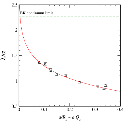
Figure 15: Approach to the continuum limit of $\lambda/\alpha$ against $a$ in units of $R_{s}$. The dashed line shows the continuum value obtained from a simulation of the BK equation. A continuum extrapolation from this alone (continuous line) appears unreliable.

It is simply the necessity of having a very large hierarchy of relevant scales $a\ll R_{s}<L$ that interferes with a continuum extrapolation. This has been found not to be specific to the JIMWLK equation but to equally affect the BK equation [35]. Comparison with BK has allowed to extend the systematics of the continuum limit more carefully using a much larger range of volumes and initial conditions with reduced errors and will be discussed in Sec. 6.3 after reviewing the size of violations of correlator factorization (97) that distinguishes JIMWLK from BK.

6.2 Size of factorization violations

A feature that allows a direct comparison of JIMWLK and BK simulations is the smallness of factorization violations in the simulations of [35].

One might expect that the BK equation to be a fairly good approximation of the JIMWLK equation, in particular if the initial conditions are uncorrelated and correspond to factorized correlators for which

$$\langle{\rm tr}(U_{\bm{x}}^{\dagger}U_{\bm{z}}){\rm tr}(U_{\bm{z}}^{\dagger}U_{\bm{z}})\rangle-\langle{\rm tr}(U_{\bm{x}}^{\dagger}U_{\bm{z}})\rangle\langle{\rm tr}(U_{\bm{z}}^{\dagger}U_{\bm{z}})\rangle$$ (233a)

or

$$\frac{\langle{\rm tr}(U_{\bm{x}}^{\dagger}U_{\bm{z}}){\rm tr}(U_{\bm{z}}^{\dagger}U_{\bm{z}})\rangle-\langle{\rm tr}(U_{\bm{x}}^{\dagger}U_{\bm{z}})\rangle\langle{\rm tr}(U_{\bm{z}}^{\dagger}U_{\bm{z}})\rangle}{\langle{\rm tr}(U_{\bm{x}}^{\dagger}U_{\bm{z}})\rangle\langle{\rm tr}(U_{\bm{z}}^{\dagger}U_{\bm{z}})\rangle}$$ (233b)

vanish. This would appear to be essentially true for generic separations as shown in Fig. 16. There, for concreteness, points are chosen so that $({\bm{x}}-{\bm{z}})\parallel\bm{e}_{1}$, $({\bm{z}}-{\bm{z}})\parallel\bm{e}_{2}$ and $|{\bm{x}}-{\bm{z}}|=|{\bm{z}}-{\bm{z}}|$. The left shows (233a) and one should recall that the natural magnitude for these correlators is $\sim 1$. The right shows a plot of (233b) based on the same simulation results with one leg kept at length 10 in lattice units and the length of the other leg on the horizontal axis. Evolution would appear to erase scaling violations in this plot. Thus, given the initial conditions used in[35], it would appear that the correlators cancel with 1–2 % accuracy, with the violations staying roughly at the same size throughout the $Y$ interval covered.

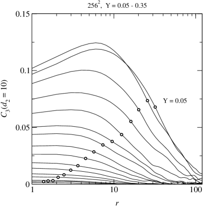
Figure 16: Factorization violations for a $4$-field correlator. The geometry is explained in the text. Unnormalized correlator (233a) on the left (from [35]). Typical error size is indicated by dashed lines for a curve in the middle. Normalized correlator (233b) on the right. The dots indicate the value of $R_{s}(Y)$ for the individual curves. Factorization violations are generically small and indicate that evolution does not induce strong violations of factorization. Consequently, the BK equation will be a good approximation as long as the initial condition does not contain strongly nonfactorizing contributions.

Recently, however, Iancu and Mueller [87] have argued that evolution builds up correlations that violate factorization. They argue that factorization violations are caused by rare configurations, build up during evolution and have the effect of reducing the evolution rate. Although this deserves further study, explicit comparison of shapes for the dipole correlator from both JIMWLK and BK simulations at same size lattices also give only very small differences. In particular, as shown in Fig. 18, one does not see strong deviations between evolution rates of JIMWLK and BK simulations on comparable lattices. This seems to indicate that these simulations in general were not sensitive to the correlations referred to in [87]. For the present purposes it would appear to be safe to conclude that for the type of initial conditions explored to date, the BK equation should give a good approximation of the salient features of the evolution. This is the basis on which BK simulations have been used to refine the understanding of the UV extrapolation by augmenting Fig. 15 with results from BK simulations in which one also uses a lattice representation for transverse space to parallel the treatment of the JIMWLK equation.

6.3 Continuum limit of BK and JIMWLK at fixed coupling

In order to study the cutoff-dependence and to facilitate the comparison with JIMWLK simulations, one best solves the BK equation with the same type of discretization in transverse space that is necessary to implement the former. This is precisely what has been done in [35].

Independent results for the continuum have been obtained by another method based on Fourier transformation presented in [61, 68]. In these approaches the kernel involves only a 1-dimensional integral for which a logarithmic momentum variable $\Xi\sim\ln k^{2}$ is used. Consequently, it becomes easy to include a very large range of momenta in the calculation; typically, more than 20 orders of magnitude are used. Thus, this allows to obtain a cutoff-independent continuum limit result for the evolution exponent $\lambda$. The key result obtained with this method was already shown in Fig. 15 for comparison with the JIMWLK extrapolation. The large range of momenta needed to get convergence is already a clear indication of what can be quantitatively seen in the discretized coordinate space version I will turn to now.

Figure 17: (From [35]) The evolution of $N({\bm{r}})$ on a $4096^{2}$ lattice, measured along on-axis direction. The curves are plotted with interval $\delta Y=0.25/\alpha$, and the total evolution time is $7/\alpha$.

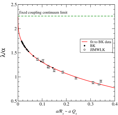
Figure 18: (From [35]) Continuum extrapolations for $\lambda$ using JIMWLK and BK simulations. The UV cutoff is plotted in units of the physical scale $R_{s}$. The continuous line is $\lambda/\alpha_{s}=2.26-2.0(a/R_{s})^{0.32}$

Fig. 18 shows the evolution of $N$ measured for a $4096^{2}$ lattice. The similarity with the dipole function obtained with the JIMWLK equation is striking, see Fig. 14. Again the initial shape settles towards the scaling form, which then continues to evolve by shifting towards smaller $R$ while preserving the shape. Nevertheless, even with a scaling form reached, the spacing of curves and hence $\lambda$ is not constant. This again is due to the growing influence of the UV cutoff.

The most sensitive quantity turns out to be $\lambda(Y)$, which in this case is free of statistical errors. A function of the form $\lambda/\alpha_{s}=c_{1}+c_{2}(a/R_{s})^{\nu}$ is an excellent fit to the data and fixes $c_{1}=2.26$, $c_{2}=2.0$ and $\nu=0.32$. The $a\rightarrow 0$ result agrees perfectly with the momentum space result although this was not included in the fit procedure. This is shown in Fig. 18. The agreement of BK and JIMWLK results at corresponding cutoff scales is remarkable over the whole range. Most striking is an evaluation of the active phase space. While on the IR side activity is limited to within one order of magnitude of the saturation scale $Q_{s}$, one needs the cutoff on the UV side to be about 6 orders of magnitude larger than $Q_{s}$ to get within 1% of the continuum value, as is easily extracted from the power law fit.

This situation is clearly unnatural: large open phase space of this magnitude usually generates large logarithmic corrections that need to be resummed to get physically reliable results. This has been used to argue that the main source for such corrections are due to running coupling effects and study the effects which, among other new qualitative features, will bring a large reduction of active phase space in the context of the BK equation that erases the potential for large logarithmic corrections.

7 Running coupling effects in the BK equation

7.1 Running coupling and UV phase space

If one wants to discuss running coupling effects and how they affect the UV behavior one has first to state that JIMWLK and thus also BK have been derived in leading logarithmic approximation and thus, contrary to state of the art BFKL calculations, one does not know what sets the scale in these evolution equations from a reliable calculation. One is therefore left with a discussion of the structure of the diagrams leading to the driving terms of the evolution equations to argue a reasonable choice. For simplicity [35] have argued and calculated in the context of the BK equation. One should always keep in mind that qualitatively these arguments will have similar implications also for the full JIMWLK treatment.

In the context of both JIMWLK and BK it is common to argue that a good scale choice is $Q_{s}(Y)$, since it is there that the r.h.s. of the evolution equation peaks. Since with this choice the scale in the coupling changes during evolution, this has often been dubbed running coupling (c.f.[55]). In fact, it is quite easy to see, that by a simple reparametrization of the $Y$ axis such a scale setting is mapped on a fixed coupling treatment, provided one uses the same initial condition. For this reason it might be less controversial to use the term scale setting in this context. To be explicit, fixed coupling and scale setting at $Q_{s}$ differ by an additional factor of $f(Y)=\frac{\alpha_{s}(Q_{s}(Y)^{2})}{\alpha_{s}^{\text{fixed}}}$ on the r.h.s. of the BK equation. If one uses $Y$ to parametrize evolution with the $Q_{s}$ scale setting and $Y^{\prime}$ in the fixed coupling case, $f(Y)$ is in fact the Jacobian $dY^{\prime}/dY$ of the reparametrization

$$Y^{\prime}-Y^{\prime}_{0}=\int\limits_{Y_{0}}^{Y}d\tilde{Y}\frac{\alpha_{s}(Q_{s}(Y)^{2})}{\alpha_{s}^{\text{fixed}}}\ .$$ (234)

This immediately leads to the conclusion that the phase space structure of the evolution equation can not differ between the two and thus, this scale choice will not cure the problems encountered above.

The difficulty can be traced to the fact that the scales in a diagram describing a single emission step during evolution for a fixed size parent dipole will generically have nothing to do with $Q_{s}$, if that parent dipole has a size very different from $1/Q_{s}$. The situation in the IR and UV (relative to $Q_{s}$) will behave very differently: While the nonlinear effects will generally block evolution in the IR, UV scales that dominate the diagrams will become visible and enter the coupling. While on this level one can not calculate (even for BK) which of the scales (the sizes of parent and daughter dipoles) or combination thereof truly enters the coupling, a scale of the order of the parent dipole size appears sensible. Like the authors of [73, 74], also[35] choose to account for running coupling effects by having the coupling run at the natural scale present in the BK-equation, the size of the parent dipole $(\bm{x}-\bm{y})^{2}$. Such a treatment is often called “DGLAP improved” if the term “running coupling” is already occupied for what is here called $Q_{s}$ scale setting. Explicitly in Eq. (98), one replaces the constant $\alpha_{s}$ by the one loop running coupling at the scale $1/(\bm{x}-\bm{y})^{2}$:

$$\alpha_{s}\to\alpha_{s}(1/(\bm{x}-\bm{y})^{2})=\frac{4\pi}{\beta_{0}\ln\frac{1}{(\bm{x}-\bm{y})^{2}\Lambda^{2}}}\hskip 28.45274pt\text{with}\hskip 28.45274pt\beta_{0}=(11N_{c}-2N_{f})/3\ .$$ (235)

$\Lambda$ in Eq. (235) is related to $\Lambda_{\text{QCD}}$ by a simple factor of the order of $2\pi$. The equation then reads

$$\partial_{Y}N_{Y;\bm{xy}}=\frac{\alpha_{s}(1/(\bm{x}-\bm{y})^{2})N_{c}}{2\pi^{2}}\int\!\!d^{2}z\ \tilde{\cal K}_{\bm{x}\bm{z}\bm{y}}\,\Big{\{}N_{Y;\bm{xz}}+N_{Y;\bm{zy}}-N_{Y;\bm{xy}}-N_{Y;\bm{xz}}N_{Y;\bm{zy}}\Big{\}}\ .$$ (236)

Such a simple replacement, of course, is not what we expect to arise from an exact calculation in which the two loop contributions that generate the running will emerge underneath the integral over $\bm{z}$. This comes on top of the fact that at next to leading order there will be corrections beyond the running coupling effects that are entirely unaccounted for by this substitution. Nevertheless, it appears natural to argue that Eq. (235), when used in the BK equation, captures the leading effect associated with the “extraneous” phase space uncovered quantitatively in Sec. 6.3. This has been the outcome of a long discussion in the context of the BFKL equation and its next to leading order corrections [88, 89, 90, 91, 92, 93, 94]. Here one simply takes this as the starting point with the attitude that a scale setting technique like the one employed in Eq. (235) is but the easiest way to get even quantitatively reliable initial results.

With running coupling implemented, one has to face the presence of the Landau pole in Eq. (235). The main point here is, that, while indeed one does not control what is happening at that scale, one is justified in providing a prescription for its treatment. With $Q_{s}\gg\Lambda_{\text{QCD}}$ the integral on the r.h.s. of the BK equation yields extremely small contributions at scales of the order of $\Lambda_{\text{QCD}}$, typically of the order of $10^{-7}$ times what is seen around $Q_{s}$. This is the reason why one is allowed to ignore whatever happens there and to freeze any correlators such as $N$ at these scales at the values provided by the initial condition. Note that the same reasoning is already necessary at fixed coupling in some sense. If one turns on running coupling, the physical thing to do is to switch off the influence of the divergence at the Landau pole, for instance by freezing the coupling below some scale $\mu_{0}$. Of course, one has to make sure that the details of where one does that will not affect the results.

Such an argument about the integrals in the BK equation is valid at zero impact parameter or infinite transverse target size, where the nonlinearity is present and sizable everywhere. For large impact parameter one necessarily enters the region where the nonlinearity is small and there one would remain sensitive to the value of $\mu_{0}$. That is the central reason for not considering such situations.

That the effects of running coupling slow down evolution has been known from the earliest numerical treatments of BK. The study of the UV phase space in [35] explicitly demonstrates the reason for this: Fig. 19 shows an example for the extrapolation of $\lambda/\alpha_{s}(Q_{s}(Y)^{2})$ to its continuum value at one value of $Y$ (corresponding to $\alpha_{s}(Q_{s}(Y)^{2})=0.2$) and compares it to the fixed coupling case shown earlier. This feature persists over a large range in $Q_{s}$ as shown in [35].

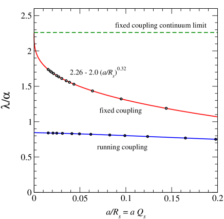
Figure 19: (From[35]) example of a continuum extrapolation of $\lambda/\alpha_{s}(Q_{s}(Y)^{2})$ for a fixed initial condition at a $Y$-value where $\alpha_{s}(Q_{s}(Y)^{2})=0.2$, compared to the fixed coupling case.

The size of active phase space becomes particularly clear in Fig. 20, which shows activity centered within an order of magnitude around $Q_{s}$. The rightmost panel shows remarkable agreement with the analytical results of Mueller and Triantafyllopoulos if their free parameter is used as a fit parameter.

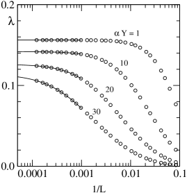
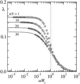
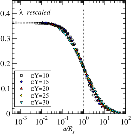
Figure 20: (From[35]) UV dependence of the BK-equation on the asymptotic line after the parent dipole scale is taken to determine the coupling. Left: $\lambda$ against $a$ in units of lattice size. Middle: $\lambda$ against $a$ in units of $R_{s}$, the natural units. Right: the same rescaled with the $Y$ dependence scaled out using the results of [73, 74], (121) and (122) with $\tilde{c}=1.5$ ($\tilde{Y}$ just leads to a reparametrization). Active phase space is limited in the UV (and IR) by $5$ to $10\times Q_{s}$.

Despite the presence of $\Lambda_{\text{QCD}}$ through the running coupling the solutions show a remarkable degree of scaling, called near scaling in [35]. Interestingly one may use the evolution rate $\lambda$ to check if this behavior is reached. Fig. 22 shows that, starting from G-B+W type initial conditions of the form

$$N_{Y_{0},{\bm{r}}}=1-e^{-{\bm{r}}^{2}Q_{s}(Y_{0})^{2}/4}\ ,$$ (237)

with different values for the characteristic scale the system quickly converges onto an asymptotic line. On this line the system shows scaling behavior to very good accuracy as illustrated in Fig. 22.

Figure 21: (From [35]) $\lambda=\partial_{Y}\ln Q_{s}(Y)$ for different initial conditions. All curves starting from Gaussian initial conditions stay below an asymptotic line along which we find (approximately) scaling dipole functions $N$.

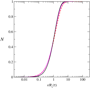
Figure 22: (From [35]) Approximate scaling behavior of $N_{Y,\bm{xy}}$ on the asymptotic line of Fig. 22.

In fact, the universal features of this equation have been studied far into asymptotic region and Fig. 23 summarizes many of the results. Fig. 23 extends the range shown in Fig.22 enormously and adds comparisons with the fixed coupling case and the analytic results of Mueller and Triantafyllopoulos. Two simple parametrizations are shown to emphasize how strong the change compared to fixed coupling is, not only in size but also in functional shape. Let me discuss these issues in turn.

Fig. 23 shows $\lambda$ plotted against $\alpha_{s}(Q_{s}^{2})$ and the fixed coupling situation will emerge in the guise of $Q_{s}$ scale setting. This is represented by the steeply rising straight line (solid) which simply corresponds to $\lambda(Y)=2.26\alpha_{s}(Q_{s}^{2})$, where the coefficient was extracted in a fixed coupling simulation. Why is this the relevant comparison? Recall the discussion of Sec. 3.4: in the fixed coupling case scaling necessarily implies that $Q_{s}$ is of the form

$$Q_{s}(Y^{\prime})=e^{\,c\>\alpha_{s}^{\text{fixed}}(Y^{\prime}-Y^{\prime}_{0})}\ Q_{s}(Y^{\prime}_{0})$$ (238)

with constant $c$. The value of $c$ is uniquely determined by the shape of the scaling solution in transverse space and turns out to be $c=2.26$. $Q_{s}$ scale setting on the other hand amounts to the reparametrization (234), and one immediately reads off how $\lambda$ changes from the fixed coupling case:

$$\lambda(Y)=\partial_{Y}\ln Q_{s}(Y^{\prime})=c\ \alpha_{s}^{\text{fixed}}\ \frac{dY^{\prime}}{dY}=c\ \alpha_{s}(Q_{s}(Y)^{2})\ .$$ (239)

$c$ remains the same constant as in the fixed coupling case and thus to the fixed coupling curve in Fig. 23. Eq. (239) implies that the form of the leading term with $c=2.26$ simply corresponds to $Q_{s}$ scale setting and thus necessarily suffers the same UV problems as the fixed coupling case.

The Mueller-Triantafyllopoulos result is shown to agree with the asymptotic line of near scaling throughout the whole range (dashed). At large $Q_{s}$ both the fixed coupling and the MT curves match up. This is due to the fact that there the MT result (which was given in Eq.(121) as a function of $Y$ instead of $Q_{s}$) at large $Y$ has an expansion in powers of $\alpha_{s}(Q_{s}^{2})$ in the form

$$\lambda(Y)=c\alpha_{s}(Q_{s}(Y)^{2})+\text{small corrections}\ .$$ (240)

This can be understood in the following way: One makes the ansatz

$$\lambda(Y):=\partial_{Y}\ln(Q_{s}(Y)/\Lambda_{\text{QCD}})=\lambda_{0}\ \big{[}\alpha_{s}(Q_{s}(Y)^{2})\big{]}^{n}\hskip 28.45274pt\alpha_{s}(Q_{s}(Y)^{2}):=\frac{4\pi}{\beta_{0}\ln(Q_{s}(Y)^{2}/\Lambda_{\text{QCD}}^{2})}$$ (241)

with $\beta_{0}=(11N_{c}-2N_{f})/3$, and finds

$$\frac{Q_{s}(Y)^{2}}{\Lambda_{\text{QCD}}^{2}}=\exp\Big{\{}\Big{[}(n+1)2\lambda_{0}\big{(}\frac{4\pi}{\beta_{0}}\big{)}^{n}(Y-Y_{0})+\big{[}\ln(\frac{Q_{s}(Y_{0})^{2}}{\Lambda_{\text{QCD}}^{2}})\big{]}^{n+1}\Big{]}^{\frac{1}{n+1}}\Big{\}}\ .$$ (242)

Recovering $\lambda$ from this leads to

$$\lambda(Y)=\frac{\lambda_{0}(\frac{4\pi}{\beta_{0}})^{n}}{\Big{[}(n+1)2\lambda_{0}(\frac{4\pi}{\beta_{0}})^{n}(Y-Y_{0})+\big{[}\ln(\frac{Q_{s}(Y_{0})^{2}}{\Lambda_{\text{QCD}}^{2}})\big{]}^{n+1}\Big{]}^{1-\frac{1}{n+1}}}\xrightarrow{n\to 1,\lambda_{0}\to 2.26}\frac{.88}{\sqrt{Y+\tilde{Y}}}$$ (243)

so that the leading term of Eq. (121) corresponds to $n=1$ as advertised, with matching numerical coefficients. [I have followed the spirit of [73, 74] and absorbed the freedom in the initial condition at $Y_{0}$ into the corresponding $\tilde{Y}$ of (121).]

This behavior at large $Y$ can also be expected for the numerical treatment through a simple extension of the scaling argument of [55]. Starting from the near scaling observation, one repeats the steps leading to Eqns. (101) and (102) and ends up with an expression for $\lambda(Y)$ of the form

$$2\pi\lambda(Y)=\frac{N_{c}}{2\pi^{2}}\int\frac{d^{2}rd^{2}z}{\bm{u}^{2}\bm{v^{2}}}\alpha_{s}(1/\bm{r}^{2})\big{(}N(\bm{u}^{2}Q_{s}^{2})+N(\bm{v}^{2}Q_{s}^{2})-N(\bm{r}^{2}Q_{s}^{2})-N(\bm{u}^{2}Q_{s}^{2})N(\bm{v}^{2}Q_{s}^{2})\big{)}+\ldots$$ (244)

in which the dots stand for the small scaling violations. The only source for the difference between the fixed coupling expression Eq. (102) and (244) or the corresponding lines in Fig. 23 lies in the ${\bm{r}}$ dependence of the running coupling that is now inside the integral. To obtain the strong relative reduction in active phase space observed in Fig. 19, $\alpha_{s}$ must vary considerably over the range of scales contributing to the integral in the fixed coupling case. Wherever this happens, $\lambda(Y)$ will be a nontrivial function of $\alpha_{s}(Q_{s}(Y)^{2})$. Conversely, at asymptotically large $Q_{s}$, where the $\alpha_{s}(1/\bm{r}^{2})$ probed in Eq. (244) turn essentially constant over a range comparable to the phase space needed in the fixed coupling case, one should return to a situation as in Eq. (240).

It is essential to remind oneself here that the limit in which the leading term of (240) is sufficient is not under control. The price to pay for this behavior at large $Y$ is the reopening of phase space to the size encountered already at fixed coupling.

As in [35], this is illustrated by tabulating (see table 1) a measurement of active phase space in terms of the values of $a/R$ needed to find $\lambda$ within a given percentage of its continuum value at different $\alpha_{s}(Q_{s}(Y)^{2})$. This is then compared with the fixed coupling result.

deviation from	$\alpha_{s}(Q_{s}^{2})=.2$	$\alpha_{s}(Q_{s}^{2})=.15$	$\alpha_{s}(Q_{s}^{2})=.12$	$\alpha_{s}(Q_{s}^{2})=.1$	fixed coupling
continuum value	$\lambda/\alpha=.845$	$\lambda/\alpha=.96$	$\lambda/\alpha=1.052$	$\lambda/\alpha=1.14$
10%	$a/R=0.17$	$a/R=0.15$	$a/R=0.12$	$a/R=0.1$	$a/R=0.0011$
5 %	$a/R=0.1$	$a/R=0.08$	$a/R=0.066$	$a/R=0.05$	$a/R=0.00013$
1 %	$a/R=0.027$	$a/R=0.015$	$a/R=0.007$	$a/R=0.0012$	$a/R=8.2\cdot 10^{-7}$

Table 1: Phase space needed to extract continuum values for $\lambda$ is reduced for larger values of the coupling. The fixed coupling situation reemerges asymptotically for large $Q_{s}$, i.e. small coupling.

In the far asymptotic region one is back to the unsatisfactory situation that important corrections are most likely missed, with the additional drawback, that now one has no real idea of what those might be. Fortunately, this would appear to occur only at such extremely large values of $Q_{s}$ that this concern is purely academic.

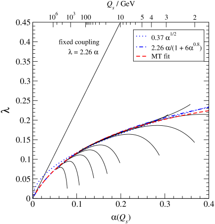
Figure 23: (From [35]) $\lambda(Y)$ as a function of $\alpha_{s}(Q_{s}(Y)^{2})$ with running coupling. A perfect overall fit is obtained with the MT result Eq. (122). The shape of the curve only depends on $\tilde{c}$, shown is a fit with $\tilde{c}=1.5$. Simple parametrizations emphasize how drastically the functional shape is changed away from a simple $c\ \alpha_{s}(Q_{s}^{2})$.

The fact that the asymptotic expansion of Mueller and Triantafyllopoulos of $\lambda(Y)$ –Eq. (121)– apparently contains only a single term beyond the questionable $Q_{s}$ scale setting result, and yet provides a fit over the whole $Q_{s}$ range with its large deviations from the leading term, may cause confusion. The resolution to this simply is hidden in the change of variables $Y$, used by MT, and $Q_{s}$, as used here. Any attempt to translate Eq. (121) from $Y$ to $Q_{s}$ or $\alpha_{s}(Q_{s}^{2})$ leads to a infinite series that will converge only slowly, so that it is in fact wrong to think of this as a single correction term from this perspective.

The discussion thus far has been about the behavior of the dipole within one of two orders of magnitude of $Q_{s}$. Careful studies have also been performed at much shorter distances [61, 95] in the scaling window, where gluon densities are still small, but scaling and the presence of $Q_{s}$ still plays an important role as it leads to behavior of the form (123) with

$${\cal G}_{Y;r,R_{s}(Y)}=C\left(\frac{{\bm{r}}^{2}}{R_{s}(Y)^{2}}\right)^{(1-{\tilde{\nu}}_{0})}\left[-\ln\frac{{\bm{r}}^{2}}{R_{s}(Y)^{2}}+\frac{1}{1-{\tilde{\nu}}_{0}}\right]\ .$$

Both studies attempt to extract the anomalous dimensions of Eq. (123), starting from distances typically a few orders of magnitude smaller than $R_{s}$.

They find that for this quantity which only makes sense at such short distances, running coupling effects remain important over an enormous range. Residual information about the initial conditions used appears to be more persistent than close to $Q_{s}$. At the same time running coupling effects remain particularly important in this range. Both these facts can be understood by looking at the BK equation at running coupling and the integral expression for $\lambda(Y)$. Writing, for instance, Eq.(236) in terms of rescaled variables $\tilde{\bm{r}}:={\bm{r}}Q_{s}(Y)$ etc. one obtains

$$\partial_{Y}N_{\tilde{\bm{r}}}=\frac{N_{c}}{2\pi^{2}}\frac{b_{0}}{\ln(\frac{Q_{s}^{2}(Y)}{\Lambda_{\text{QCD}}^{2}})-\ln(\tilde{\bm{r}}^{2})}\int\!\!d^{2}\tilde{z}\ \tilde{\cal K}_{\tilde{\bm{x}}\tilde{\bm{z}}\tilde{\bm{y}}}\,\Big{\{}N_{\tilde{\bm{u}}}+N_{\tilde{\bm{v}}}-N_{\tilde{\bm{r}}}-N_{\tilde{\bm{u}}}N_{\tilde{\bm{v}}}\Big{\}}\ .$$ (245)

Clearly, with increasing $Q_{s}$ the importance of running coupling effects (in the sense that goes beyond $Q_{s}$ scale setting) will be pushed further and further away from the scaling region where $\tilde{\bm{r}}={\bm{r}}Q_{s}(Y)\gtrsim 10^{-2}$, while at shorter distances, where the anomalous dimensions are measured form a scaling fit to (123), $\tilde{\bm{r}}$ dependence of the coupling remains important. These features are reflected by the numerical results of [61, 95] which emphatically confirm the existence of the scaling window: they cannot even find any evidence that scaling of the form (123) would break down at the upper end of the scaling region.

To summarize the results of this section, one should state that with parent dipole running, the contributions to $\lambda$ arise from within little more than an order of magnitude of the saturation scale, as Fig. 20 shows impressively. [This concerns the region in cutoffs over which there is an appreciable change in the value extracted.] This indicates that the dominant phase space corrections are indeed taken into account and the basic physics ideas that had initially motivated the density resummations are realized. While the IR side of the resummation was working already at fixed coupling, the UV side of phase space is only tamed if the coupling runs at a scale directly visible in the diagrams comprising the r.h.s. of the evolution equation such as $1/\bm{r}^{2}$, the parent dipole size. This is equivalent to incorporating subleading terms in the asymptotic expansions (240) at least to the order done by Mueller and Triantafyllopoulos in (121). Only with both the nonlinearities and a running coupling that goes beyond $Q_{s}$ scale setting in the sense explained above are we justified to claim that the evolution is dominated by distances of the order of $R_{s}$ and thus the coupling involved in typical radiation events during evolution is of order $\alpha_{s}(Q_{s}(Y)^{2})$. [Emission from very small dipoles would simply not be sufficiently suppressed with $Q_{s}$ scale setting.] While the result of [73, 74] provides a physically motivated explanation of the curve, a convenient way to convert this into an explicit function of $Q_{s}(Y)$ does not exist. For this purpose the fits shown in Fig. 23 provide a useful, quantitative, rule-of-thumb representation for the numerical result. The existence of the scaling window is numerically confirmed: Scaling features extend into the low density region and persist throughout the scaling window to distances much shorter than the saturation scale.

7.2 Evolution induces longitudinal correlations: breaking of $A^{\frac{1}{3}}$-scaling in DIS

Already in the introduction it has been argued and illustrated in Fig. 8 that for uncorrelated scattering centers $Q_{s}$ should scale with larger atomic number like $A^{1/3}$ as shown in Eq. (9). This has recurred in the context of the MV model and its generalizations (Sec.2.2): generically one expects that going to larger nuclear targets ought to have an enhancing effect on the importance of the nonlinearities encountered. To recall the argument: If one is at small enough ${x_{\text{bj}}}$ (high enough energies) for the projectile to punch straight through the target, going to a larger target means interaction with more scattering centers as indicated in Fig. 5. Taking these to be color charges located in individual nucleons inside the target nucleus the interaction will occur with more and more uncorrelated color charges the larger the target. Viewed from up front this amounts to a smaller correlation length in the transverse direction. In terms of $Q_{s}$ this would lead to a variant of relation (9),

$$Q_{s}^{A}(Y)^{2}=cA^{\frac{1}{3}}Q_{s}^{p}(Y)^{2}$$ (246)

where $c$ is some, yet unspecified constant that takes into account nontrivial geometry and other issues not incorporated in the McLerran-Venugopalan model (see also the discussion below Eq. (28) and [42]). Note that none of these arguments would give a clear delineation of the range of $Y$ values for which this would be appropriate. It is clear, however, that in the context of small ${x_{\text{bj}}}$ evolution such a statement becomes even less trivial: the whole idea of deriving a small ${x_{\text{bj}}}$ evolution equation is based on the premise that the logarithmic corrections determining the evolution step are entirely target independent. The only place where target dependence is allowed to enter is the initial condition as already indicated in Eq. (9). A careful determination of $c$ can not be done without phenomenological effort, but a discussion of how evolution changes such a relationship can be done on the basis of the evolution equations alone. This is what I focus on here.

In simple cases the two notions –evolution and scaling at all $Y$– are not conflicting with each other: indeed a rescaling like in Eq. (246) is fully compatible with fixed coupling evolution on the asymptotic line, where (in the continuum limit)

$$Q_{s}(Y)=e^{\lambda(Y-Y_{0})}Q_{s}(Y_{0})$$ (247)

with a universal value for $\lambda$, so that a simple rescaling of the properties of the initial condition according to

$$Q_{s}^{A}(Y_{0})^{2}=cA^{\frac{1}{3}}Q_{s}^{p}(Y_{0})^{2}\$$ (248)

automatically yields Eq. (246) at all $Y$ declaring it fully compatible with evolution.

At running coupling, however, this ceases to be the case. The straightforward physical argument is that evolution is characterized by $\alpha_{s}(Q_{s}^{2})$, which initially is larger for protons than for nuclei, because of the difference in saturation scales at the initial condition. In this situation evolution will be faster for smaller targets and eventually catch up with that of the larger ones.

Technically, with running coupling (and again on the asymptotic line), one finds a $Y$ dependent $\lambda$ that may be parametrized through some function $f$ of $\alpha_{s}(Q_{s}(Y)^{2})$ as in the previous section:

$$\lambda(Y)=\partial_{Y}\ln Q_{s}(Y)=f(\alpha_{s}(Q_{s}(Y)^{2}))\ .$$ (249)

In this generic case

$$Q_{s}(Y)=e^{\int^{Y}_{Y_{0}}dY^{\prime}f(\alpha_{s}(Q_{s}(Y)^{2})}Q_{s}(Y_{0})$$ (250)

and a rescaling of $Q_{s}^{p}(Y_{0})^{2}$ will not simply factor out as in Eq. (247). Therefore a simple rescaling like Eq. (246) will conflict with evolution. All phenomenological fit functions encountered in Fig.23 share this property, which is at the heart of the reasoning used by Mueller in [96] to argue that evolution will eventually erase $A$-dependence in $Q_{s}$.

Instead of a numerical analysis (c.f. [95]) and purely to illustrate the point, one may trace the memory loss with a simple parametrization like Eq. (241), equivalent to a $Y$ dependence of $Q_{s}$ according to Eq. (242). Recall that for $n=1/2$ this should be even quantitatively correct over the physically interesting domain.

Scaling in the $A$-dependence at $Y_{0}$ according to $Q_{s}^{A}(Y_{0})^{2}=cA^{\frac{1}{3}}Q_{s}^{p}(Y_{0})^{2}\$, one uses Eq. (242) to predict the combined $Y$ and $A$ dependence of the saturation scale. The result is in qualitative agreement with [96]: the ratio of saturation scales in the bulk of the region shown in Fig. 23 behaves like

$$\frac{Q^{A}_{s}(Y)^{2}}{Q^{p}_{s}(Y)^{2}}=\frac{\exp{\Big{[}(n+1)2\lambda_{0}\big{(}\frac{4\pi}{\beta_{0}}\big{)}^{n}(Y-Y_{0})+\big{[}\ln(\frac{cA^{\frac{1}{3}}Q_{s}(Y_{0})^{2}}{\Lambda_{\text{QCD}}^{2}})\big{]}^{n+1}\Big{]}^{\frac{1}{n+1}}}}{\exp{\Big{[}(n+1)2\lambda_{0}\big{(}\frac{4\pi}{\beta_{0}}\big{)}^{n}(Y-Y_{0})+\big{[}\ln(\frac{Q_{s}(Y_{0})^{2}}{\Lambda_{\text{QCD}}^{2}})\big{]}^{n+1}\Big{]}^{\frac{1}{n+1}}}}\xrightarrow{Y\to\infty}1\ .$$ (251)

This is plotted in Fig. 24 over a very large range in $Y$. Clearly larger nuclei suffer stronger initial “erasing.” It should be kept in mind that realistically one should not expect real world experiments to cover more than a few orders of magnitude in ${x_{\text{bj}}}$ and thus a small interval in $Y-Y_{0}$.

Figure 24: (From[35]) $A$-dependence for proton saturation scales from $1$ to $100$GeV. $c$ parametrizes possible shape dependence as explained in the text.

8 A brief foray into phenomenology

Phenomenology in the context of the color glass condensate is a very hot topic, in particular in connection with present activities at RHIC. As a consequence, many of the topics are not yet settled enough to be included in a review. Nevertheless, this review would be incomplete without trying to give a flavor of the ideas and experiments being discussed.

The key point in all of them is the appearance of $Q_{s}$ and associated scaling in the interpretation of experimental data. This is done with respect to the ${x_{\text{bj}}}$ dependence as well as the $A$ dependence where available, both in the saturation region and the scaling window.

The prime example still is the application of saturation ideas to HERA data at ${x_{\text{bj}}}<10^{-2}$. This will be the first topic discussed below in Sec. 8.1.

Nucleus nucleus collisions form a much more complicated environment than lepton nucleus collisions and the step from fully developed theory to comparison with data is much larger.

There is one approach to heavy ion data which is directly build on the technology described in this review, and that aims at the initial condition of heavy ion collisions. This will be briefly touched upon in Sec. 8.2.

A different approach based on $({\bm{k}}=)$ $k_{T}$-factorized formulae for particle production in terms of unintegrated gluon densities as defined in Eq. (42) [85, 97, 98, 99, 100, 61, 101, 102], allows to apply the results of the evolution equations to $AA^{\prime}$ experiments:

$$E{d\sigma\over d^{3}p}={4\pi N_{c}\over N_{c}^{2}-1}\ {1\over{\bm{p}}^{2}}\ \times\,\int^{\bm{p}}\,d{\bm{k}}^{2}\,\alpha_{s}\ \varphi_{A}({x_{\text{bj}}},{\bm{k}}^{2})\ \varphi_{A^{\prime}}({x_{\text{bj}}}^{\prime},({\bm{p}}-{\bm{k}})^{2})\ .$$ (252)

Despite some obvious shortcomings concerning perturbative and hadronization corrections, a treatment based on this formula is currently the best one can do. Keeping this in mind, the formula imprints the consequences of any $Q_{s}$ scaling found in unintegrated distributions onto transverse momentum spectra in nucleus nucleus collisions.

A very illustrative example in this context is the Cronin effect and its expected behavior under evolution discussed in Sec. 8.3. Particle multiplicities are another example, but indications are that this topic will come into its full right only with LHC energies. These and other ideas relevant to build a solid understanding on how and exactly in which kinematical domain the CGC shows up in experiments will briefly reappear in Sec. 8.4.

8.1 Geometric scaling in HERA and lepton nucleus collisions

The discovery of geometric scaling in HERA data at ${x_{\text{bj}}}<10^{-2}$ as prompted by the Golec-Biernat and Wüsthoff fit [32, 34] was the first phenomenological application of saturation ideas in small ${x_{\text{bj}}}$ physics, predating all the theoretical developments around JIMWLK and BK evolution equations that demonstrated the scaling features of these evolution equations. It brought with it the by far most efficient parametrization of HERA data at ${x_{\text{bj}}}<10^{-2}$. Recall the DIS cross section formula from the introduction (with the momentum fraction integral restored):

$$\sigma_{\mathrm{tot}}(Y,Q^{2}) = \int d^{2}{\bm{r}}\int\limits^{1}_{0}\!d\alpha\ |\psi_{\gamma^{*}}(\alpha,{\bm{r}}^{2},Q^{2})|^{2}\ \sigma_{\mathrm{dipole}}(Y,{\bm{r}}^{2})$$ (253)

where $\alpha$ is the longitudinal momentum fraction of the $q$ or $\bar{q}$, and $\bm{z}$ their relative transverse separation. $Q^{2}$ and ${x_{\text{bj}}}$-dependence is clearly separated into wave function and dipole cross section respectively. The G-B+W fit parametrizes the latter via an ${x_{\text{bj}}}$-dependent saturation scale $Q_{s}$ according to (46) and a normalization factor to carry the dimensions from the impact parameter integral:

$$\sigma_{\text{dipole}}(Y,r^{2})=\int d^{2}b\ \langle\frac{{\rm tr}(1-U_{\bm{x}}U^{\dagger}_{\bm{y}})}{N_{c}}\rangle_{Y}\hskip 28.45274pt\xrightarrow{\text{ G-B+W }}\hskip 28.45274pt\sigma_{0}(1-e^{-{\bm{r}}^{2}Q_{s}^{2}(Y)/4})\ .$$ (254)

At the same time they preempted the fixed coupling scaling form for $Q_{s}$ of Eq. (103), $Q_{s}(Y)=e^{\lambda(Y-Y_{0})}Q_{s}(Y_{0})$ $=({x_{\text{bj}}}_{0}/{x_{\text{bj}}})^{\lambda}Q_{s}(x_{0})$. This fit ansatz is just a particular realization of the scaling behavior later found to result from JIMWLK and BK, both at fixed and running coupling. Successful saturation based fits incorporating scaling forms like (123) have also been performed in the meantime [103]. The most important phenomenological result, however, is independent of the exact shape of the dipole cross section, it is the simple fact that HERA data show geometric scaling. Once the dipole cross section depends on ${x_{\text{bj}}}$ only via $Q_{s}(Y)$ as $\sigma_{\text{dipole}}(Y,{\bm{r}}^{2})=\sigma_{\text{dipole}}({\bm{r}}^{2}Q_{s}^{2}(Y))$, geometric scaling emerges directly. Rescaling the $r$ integral in Eq.(253) and using the fact that the wave function factor scales like $f({\bm{r}}^{2}Q^{2})/{\bm{r}}^{2}$, this implies

$$\sigma_{\mathrm{tot}}(Y,Q^{2})=\sigma_{\mathrm{tot}}\Big{(}Y_{0},\frac{Q^{2}}{Q_{s}^{2}(Y)}Q_{s}^{2}(Y_{0})\Big{)}$$ (255)

and should allow to map all the cross section data onto a single scaling curve. This is shown in Fig. 25

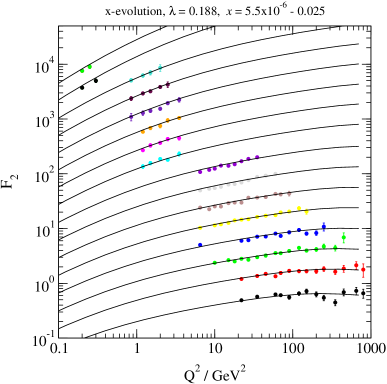
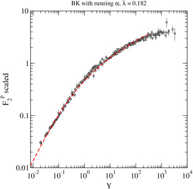
Figure 25: Geometric scaling in HERA data. Shown is the structure function $F_{2}$, which at small ${x_{\text{bj}}}$ is simply related to the cross section by a rescaling by $Q^{2}$: $\sigma(Y,Q^{2})\sim F_{2}(Y,Q^{2})\cdot Q^{2}$.

While the explicit parametrizations shown in Fig. 25 make use of BK evolution results from [35], this is not essential, at least for the scaling plot on the right. In fact, successful fits of HERA data based on CGC evolution exist [67, 103] and they are of a quality comparable to that of DGLAP fits. It is not the quality of the fit to the data (leaving aisde comments on negative gluon distributions often seen in global DGLAP analyses) that distinguishes the CGC perspective, it is the natural emergence of $Q_{s}$ and the scaling features which set it apart. Scaling features have since been looked for also in older NMC [104] and E665 [105, 106] data for the ratios of nuclear to deuterium structure functions $2F_{2}^{A}/AF_{2}^{D}$. Despite the fact that both ${x_{\text{bj}}}$ and $Q^{2}$ ranges are such that CGC saturation arguments remain marginal despite the moderate enhancement via $A$, both [107] and [108] find that scaling in both ${x_{\text{bj}}}$ and $A$ holds surprisingly well. The scaling in $A$ was fitted with a fixed power close to $1/3$ ignoring the refinements of Sec. 7.2. Due to the limited range in ${x_{\text{bj}}}$ this can not be taken as an experimental confirmation of CGC physics – such would require a measurement of ${x_{\text{bj}}}$ dependence and this is clearly a reason to explore this question more closely in experiments at higher energies. This is being actively pursued. One of the options is the Electron Ion Collider (EIC) in planning at BNL [109] as a machine dedicated to such experiments or via $pA$ collisions at the LHC where higher energies are available at the price of a more complicated projectile.

8.2 Gluon production in the initial stages of heavy ion collisions

The evolution equations have mainly been discussed in the context of $eA$ collisions, but it should be intuitively clear that a new perturbatively large scale $Q_{s}$, present in the nuclear wave function at small ${x_{\text{bj}}}$, would also manifest itself in $AA^{\prime}$ collisions. The original idea is laid out in [23], where the incoming nuclei are treated as sources of strong color fields in the spirit of the MV model. While the nonlinear nature of the fields does not allow to simply add them, it is still possible to add the color currents that create them and then to solve the resulting Yang Mills equations. This will only modify the solutions after they are in causal contact, i.e. in the forward lightcone of the collision point. At the edge of this forward cone the fields generated by the individual nuclei serve as an initial condition for what happens after the collision for a given source configuration. The source configurations themselves are subject to ensemble averaging, say with (29) (per nucleus), if one stays within the MV model or with the corresponding field averages expressed alternatively via $b$, $\alpha$ or $U$, if one goes beyond this model to incorporate ${x_{\text{bj}}}$ dependence via BK or JIMWLK equations.

[23] provides the generic framework but only attempts perturbative solutions valid for large times, however, the field equations for large densities are truly nonlinear in the very initial stages of the collision of interest. In this region numerical methods are required. These have been developed and used by [110, 111]. More recent work discusses the possibility to create “elliptic flow” [112, 113] and independent checks have been provided in [114]. The main interest of such studies is the creation of high density effects in the very initial stages of heavy ion collisions, which would appear to be necessary to explain the very short equilibration times often quoted as necessary to explain the collective phenomena supported by data.

8.3 Evolution erases the Cronin effect

The last experimental topic to be discussed here that has met with strong interest is the question for the energy dependence of what is known as the Cronin effect. I should begin this section with the warning that all input and results in terms of the CGC are formulated on a partonic level, while the underlying definitions of cross sections (256) and actual measurements are done on a hadronic level. There are strong indications that there may by important contributions from hadronization to the measured quantities. For this reason one might want to talk about what is discussed below as a Cronin-like effect. Nevertheless, the main message that small ${x_{\text{bj}}}$ evolution has a specific and rather strong effect on transverse momentum spectra remains an exciting result.

The Cronin effect refers to an enhancement of the number of particles produced in the intermediate transverse momentum range of nucleus nucleus collisions over those in proton proton collisions which is commonly attributed to a momentum broadening due to multiple rescatterings in the final state. At first sight this would appear to be at odds with the ideas of saturation which would lead to the expectation that particle production should be suppressed for momenta below $Q_{s}$ and even, as argued by [115] within the entire scaling window. This, however, is but less than half the picture.

The first observation is that the original MV model does contain Cronin type enhancement[49, 116, 117]. This is based on a sum rule [43] for the gluon distribution in the MV model that equates the total number of gluons in a (large) nucleus with $A$ times that of a nucleon. At the same time the momentum spectrum is distorted by eikonalization: small momenta are indeed depleted, while at very large momenta a perturbative $1/{\bm{k}}^{2}$ tail remains undisturbed. This can be readily recovered from (44) together with (45) under the assumption of $A^{1/3}$ scaling of the exponent in either gluon distribution or dipole cross section. (The remaining $A^{2/3}$ comes from the $d^{2}b$ integral as a global prefactor.) By necessity the “excess” has to accumulate at moderate transverse momenta which leads to Cronin enhancement.

The second observation comes from the fact that the sum rule is broken by evolution. One aspect of this is simply the modification of $A$-dependence of the saturation scale through evolution reviewed in Sec. 7.2. The effect on the gluon distribution and thus the Cronin effect is even much more pronounced: The Cronin peak is suppressed over a very short range in rapidity.

The underlying object measured is a ratio $R_{AB,CD}(Y,{\bm{p}},{\bm{b}})$ that compares numbers of produced particles per rapidity $Y$ (i.e. $Y$ for present purposes), transverse momentum $\bm{p}$ and centrality $\bm{b}$ in the collision of two nuclei $A,B$ with the same in the collision of another pair $C,D$ as a function of transverse momentum, both normalized to the number of collisions $N_{\text{coll}}(b)$:

$$R_{\text{A B;C D}}(Y,{\bm{p}},{\bm{b}})\,:=\,\frac{\langle N_{\text{coll}}(b)\rangle_{C+D}}{\langle N_{\text{coll}}(b)\rangle_{A+B}}\,\frac{dN_{A+B}/dY\,d^{2}{\bm{p}}\,d^{2}{\bm{b}}}{dN_{C+D}/dY\,d^{2}{\bm{p}}\,d^{2}{\bm{b}}}\,.$$ (256)

For practical measurements (256) is too differential and so simplified variants are used. On the one hand, there is the ratio $R_{\text{A B}}$ in which the multiplicities of (256) are integrated over impact parameter $\bm{b}$, and $C,D$ are both taken to be protons for reference. This is the standard way to show the Cronin effect. On the other hand, there is $R_{\text{cp}}$ ($c,p$ stand for central and peripheral respectively) in which $(A,B)=(C,D)$ and the multiplicities in numerator and denominator are integrated over central and peripheral regions respectively. [The same applies to the average number of collisions used to normalize.] Both quantities should show similar trends, loosely speaking, the peripheral region looks like a collision with a smaller nucleus.

$R_{\text{d Au}}$ had been studied carefully in the context of the BK equations in [69]. For this theoretical study initial conditions of the form (44) together with (45) were used to provide an initial condition that shows Cronin enhancement. The result is shown in Fig. 26 and shows the fast disappearing Cronin enhancement. Again evolution is considerably slower in the running coupling case.

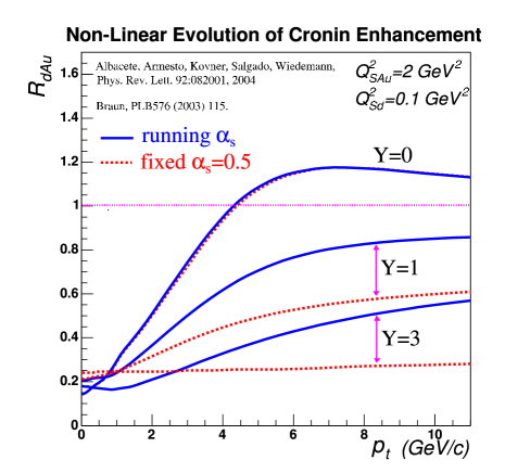
Figure 26: (Courtesy of the authors of [69]) Suppression of the Cronin peak through BK evolution both at fixed and running coupling. Running coupling evolution is slower than the fixed coupling case as seen already for generic quantities in Sec. 7.

Both $R_{\text{d Au}}$ and $R_{\text{cp}}$ have been measured by the BRAHMS experiment at RHIC [118] and are shown in Fig. 27, top and bottom strips respectively.

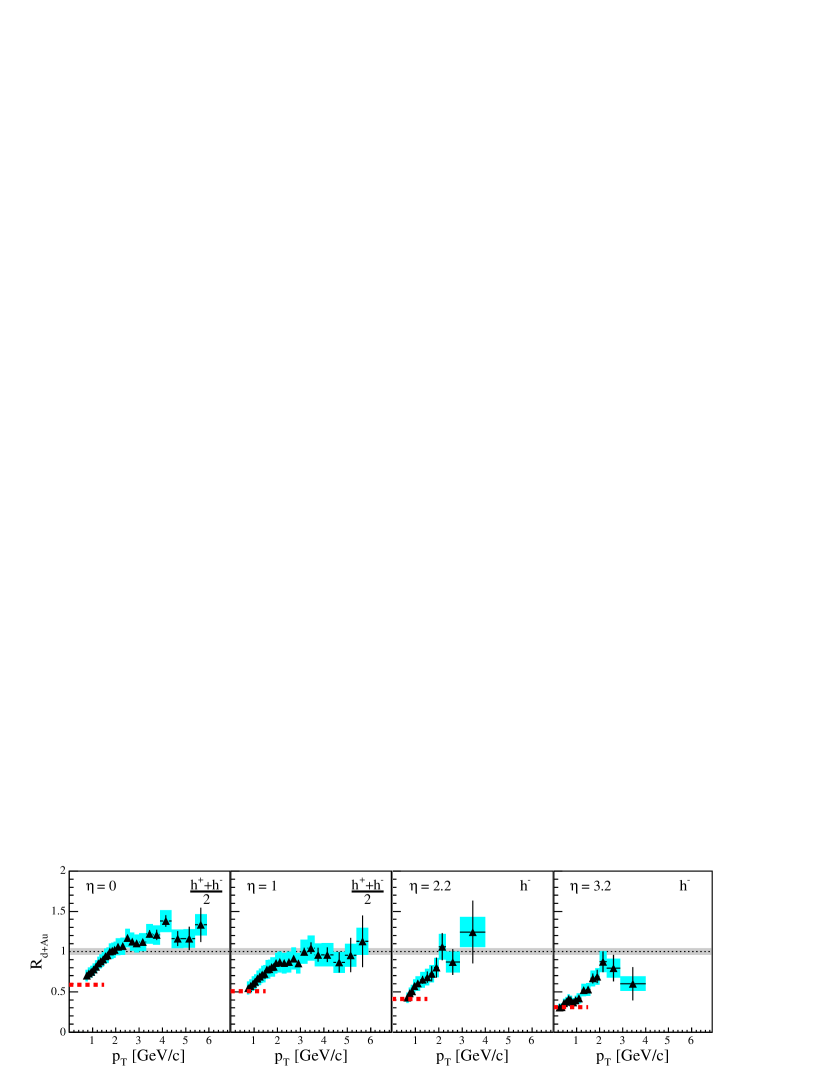
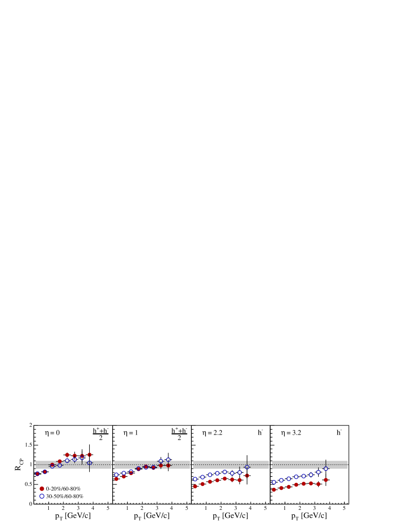
Figure 27: Brahms data [118], Top strip: $R_{\text{d Au}}$ as a function of ${\bm{p}}=p_{T}$ for different pseudorapidities $\eta$ (here to be identified with $Y$). Bottom strip: The same for $R_{\text{cp}}$ in d + Au.

In both of these measurements it is the depletion at forward rapidities that is the interesting effect: Other approaches [119, 120] that concentrate on multiple scattering to reshuffle particles in the momentum distributions typically do not take into account the nonlinearity of the small ${x_{\text{bj}}}$ evolution equation which leads to the effect shown in Fig. 26. Instead the Cronin enhancement tends to increase, reflecting the increasing number of scattering centers at small ${x_{\text{bj}}}$.

Experimental work and theoretical discussion on this topic is still ongoing, see for example [121] for a recent fit of available data.

8.4 Many ideas abound

The list of ideas given above is by no means exhaustive. The effect of $Q_{s}$ on particle multiplicities in $pA$ and $AA^{\prime}$ collisions has been discussed as well, initially for RHIC, where they have been essentially ruled out for the central rapidity region. This is in keeping with the tentative interpretation of BRAHMS data discussed in Sec. 8.3, but judging from the same data, one would expect this to be highly relevant at the LHC at central rapidities for which predictions exist [122]. The applications typically combine methods to calculate particle yields with classical Glauber formulae for multiple scattering situations –used in order to understand the reaction geometry– with a factorized ansatz for inclusive production in terms of the unintegrated gluon densities of the participants as discussed in Eq. (252). The latter are then parametrized using information about the CGC, typically with some parametrizations for the energy dependence of the saturation scale. This should give first ideas about the effects to be expected, but clearly could profit from a closer integration with the evolution equations and the concepts of Sec. 8.2.

Recently two particle and jet azimuthal corrections have been suggested [123, 124] to further study the onset of parton saturation suggested by the BRAHMS data, ideas to measure the transverse size of the area populated by gluons have been formulated [125] and too many others to give a complete list of.

It is clear, however, from the added number of theoretical complications in heavy ion experiments that a lepton nucleus experiment at high energies would be an important tool to get a clean baseline for all the applications to these more complicated experiments. This is the goal of the EIC project currently in the planning stage at BNL.

9 Conclusions

The concepts to describe saturation effects in small ${x_{\text{bj}}}$ have come a long ways since the early discussions sparked by the Gribov-Levin-Ryskin (GLR) equation [126]. Stages on the way are represented by the Mueller-Qiu[16] equation (aiming at the same double logarithmic limit as the GLR equation), Mueller’s original dipole model[17, 18, 127, 128] designed to give evolution towards small ${x_{\text{bj}}}$ and the McLerran-Venugopalan model meant to describe density effects at small but fixed ${x_{\text{bj}}}$ in large nuclei.

JIMWLK and BK evolution equations have provided a new framework, derived from small coupling QCD, that allows to take into account gluon induced density effects at small ${x_{\text{bj}}}$.

The theoretical treatment contains two types of nonlinearities, eikonalization of “soft” gluon fields into path ordered exponentials or Wilson lines as a first stage and a second stage that even exponentiates these objects –inside of shower operators– to describe emission of “hard” gluons.

The first stage is sufficient to obtain bounded results for cross sections as evidenced by the dipole formula for the DIS example (5) or Sudakov form factors in jet observables. Such expressions, since bounded, are always efficiently parametrized as exponentials as in Eqns. (35), without any reference to a specific averaging procedure for the gluon fields – interpretation in terms of a saturation scale as in Eq. (44) is most natural in the small ${x_{\text{bj}}}$ context.

The second stage exponentiation via the shower operators [54] implements ${x_{\text{bj}}}$ dependence of objects like the photon wavefunction in DIS. Via translation through Langevin formulations[13, 75] and JIMWLK equation [7, 8, 9, 10, 11, 12, 13, 14, 15], this generates an infinite hierarchy of coupled equations for cross sections, the Balitsky hierarchy, which reduces to the BK equation, if correlators factorize into two point functions.

In whichever guise this is presented, the ${x_{\text{bj}}}$ dependence is characterized by the emergence of scaling: universal behavior that ties the ${x_{\text{bj}}}$ dependence to dependence on the saturation scale.

The evolution equations impose this behavior quite quickly: Near the saturation scale details about initial conditions are efficiently erased, as is evidenced by the quick convergence onto the near scaling curve shown by the plot of the evolution rate $\lambda(Y)=\partial_{Y}\ln Q_{s}(Y)$ in Fig. 23. Once near scaling is reached, the scaling form only changes very slowly – scale breaking is present but weak[107]. This feature also manifests itself in other quantities such as, for example, anomalous dimensions as measured from BK evolution by [61, 95]. A subtlety that was manifest –although unappreciated– already in numerical simulations at fixed coupling is the importance of running coupling to tame UV phase space. Only with running coupling implemented is the evolution activity centered around the physical scale $Q_{s}$.

The generic structures of the phase space diagram Fig. 4 with saturation, scaling and extended scaling region have all been seen numerically. The perhaps simplest physical interpretation is this: Starting from a dipole function that is saturated at large dipole sizes and perturbatively small at small dipole sizes, evolution is driven by contributions from small sizes. This follows the BFKL pattern of exponential growth. Creation of large objects that would fall into the already saturated domain is prohibited by the nonlinearities, corresponding contributions are absorbed by the medium. Due to the growth at small distances, densities rise also there and the boundary where the nonlinearities start to act readjust. This happens selfconsistently in JIMWLK and BK. In [73, 74] the picture is taken literally and an even quantitatively comparable result is achieved by combining BFKL evolution with an absorptive boundary which is selfconsistently adjusted to limit growth. This type of analysis leads to scaling forms for the dipole cross section valid at small distances, and predicts the size of the scaling window via the corresponding BFKL diffusion radius.

Scaling features as found in these evolution equations had been seen earlier in HERA data at small ${x_{\text{bj}}}$ and called geometric scaling. This has encouraged phenomenological applications to various observables like particle multiplicities or the Cronin effect. Besides its ${x_{\text{bj}}}$ dependence, the $A$ dependence of $Q_{s}$ as implied by the MV model and somewhat modified by evolution [96, 35, 95] is an interesting tool to tie together experimental results in lepton proton, lepton nucleus, and nucleus nucleus experiments. While qualitative features in existing experiments –HERA and RHIC featuring most prominently on this list– appear to be compatible with state of the art CGC phenomenology, matters are far from settled. Experiments at smaller ${x_{\text{bj}}}$, like the LHC, and simpler environments, like the EIC with its electron projectiles, are needed to fully clarify the situation. Current experimental activities at RHIC and phenomenological work to match and assess the enormous amount of new results, for example by suggesting new measurements and phenomenological consequences, are very encouraging.

At the same time it would help to close the gap between reliable theory and phenomenological applications. Our understanding of small ${x_{\text{bj}}}$ evolution equations at this point is limited to the central part of lepton nucleus collisions. The technological tools and insights gained through comparison with soft emission phenomena in non-global jet observables should allow to formulate new, IR safe observables together with the associated evolution equations also in the small ${x_{\text{bj}}}$ case. This field has matured from its origins, but new developments are just around the corner.

Acknowledgement:

I whish to thank DFG and BMBF for financial support during later stages of my involvement with this topic. I am grateful to Andreas Schäfer for feedback on the first part of this manuscript, to Dionysis Triantafyllopoulos and Edmond Iancu for comments on the sections on the MT model and the scaling region as well as to Urs Wiedemann for his input on the presentation of the Cronin effect.

References

- [1] Y. Y. Balitsky and L. N. Lipatov Sov. J. Nucl. Phys. 28 (1978) 822.
- [2] L. N. Lipatov Sov. J. Nucl. Phys. 23 (1976) 642.
- [3] E. A. Kuraev, L. N. Lipatov, and V. S. Fadin Sov. Phys. JETP 44 (1976) 443–450.
- [4] E. A. Kuraev, L. N. Lipatov, and V. S. Fadin Sov. Phys. JETP 45 (1977) 199–204.
- [5] L. N. Lipatov Sov. Phys. JETP 63 (1986) 904.
- [6] M. Froissart Phys. Rev. 123 (1961) 1053–1057.
- [7] J. Jalilian-Marian, A. Kovner, L. D. McLerran, and H. Weigert Phys. Rev. D55 (1997) 5414–5428, [hep-ph/9606337].
- [8] J. Jalilian-Marian, A. Kovner, A. Leonidov, and H. Weigert Nucl. Phys. B504 (1997) 415–431, [hep-ph/9701284].
- [9] J. Jalilian-Marian, A. Kovner, A. Leonidov, and H. Weigert Phys. Rev. D59 (1999) 014014, [hep-ph/9706377].
- [10] J. Jalilian-Marian, A. Kovner, and H. Weigert Phys. Rev. D59 (1999) 014015, [hep-ph/9709432].
- [11] J. Jalilian-Marian, A. Kovner, A. Leonidov, and H. Weigert Phys. Rev. D59 (1999) 034007, [hep-ph/9807462].
- [12] A. Kovner, J. G. Milhano, and H. Weigert Phys. Rev. D62 (2000) 114005, [hep-ph/0004014].
- [13] H. Weigert Nucl. Phys. A703 (2002) 823–860, [hep-ph/0004044].
- [14] E. Iancu, A. Leonidov, and L. D. McLerran Nucl. Phys. A692 (2001) 583–645, [hep-ph/0011241].
- [15] E. Ferreiro, E. Iancu, A. Leonidov, and L. McLerran Nucl. Phys. A703 (2002) 489–538, [hep-ph/0109115].
- [16] A. H. Mueller and J.-w. Qiu Nucl. Phys. B268 (1986) 427.
- [17] A. H. Mueller Nucl. Phys. B415 (1994) 373–385.
- [18] A. H. Mueller and B. Patel Nucl. Phys. B425 (1994) 471–488, [hep-ph/9403256].
- [19] L. D. McLerran and R. Venugopalan Phys. Rev. D49 (1994) 2233–2241, [hep-ph/9309289].
- [20] L. D. McLerran and R. Venugopalan Phys. Rev. D49 (1994) 3352–3355, [hep-ph/9311205].
- [21] L. D. McLerran and R. Venugopalan Phys. Rev. D50 (1994) 2225–2233, [hep-ph/9402335].
- [22] A. Ayala, J. Jalilian-Marian, L. D. McLerran, and R. Venugopalan Phys. Rev. D52 (1995) 2935–2943, [hep-ph/9501324].
- [23] A. Kovner, L. D. McLerran, and H. Weigert Phys. Rev. D52 (1995) 6231–6237, [hep-ph/9502289].
- [24] A. Ayala, J. Jalilian-Marian, L. D. McLerran, and R. Venugopalan Phys. Rev. D53 (1996) 458–475, [hep-ph/9508302].
- [25] Y. V. Kovchegov Phys. Rev. D54 (1996) 5463–5469, [hep-ph/9605446].
- [26] I. Balitsky Nucl. Phys. B463 (1996) 99–160, [hep-ph/9509348].
- [27] Y. V. Kovchegov Phys. Rev. D55 (1997) 5445–5455, [hep-ph/9701229].
- [28] I. Balitsky hep-ph/9706411.
- [29] A. H. Mueller Nucl. Phys. B558 (1999) 285–303, [hep-ph/9904404].
- [30] Y. V. Kovchegov Phys. Rev. D61 (2000) 074018, [hep-ph/9905214].
- [31] A. Kovner and J. G. Milhano Phys. Rev. D61 (2000) 014012, [hep-ph/9904420].
- [32] K. Golec-Biernat and M. Wüsthoff Phys. Rev. D59 (1999) 014017, [hep-ph/9807513].
- [33] K. Golec-Biernat and M. Wüsthoff Phys. Rev. D60 (1999) 114023, [hep-ph/9903358].
- [34] A. M. Stasto, K. Golec-Biernat, and J. Kwiecinski Phys. Rev. Lett. 86 (2001) 596–599, [hep-ph/0007192].
- [35] K. Rummukainen and H. Weigert hep-ph/0309306.
- [36] E. Iancu, A. Leonidov, and L. McLerran hep-ph/0202270.
- [37] E. Iancu and R. Venugopalan hep-ph/0303204.
- [38] A. Hebecker and H. Weigert Phys. Lett. B432 (1998) 215–221, [hep-ph/9804217].
- [39] W. Buchmuller and A. Hebecker Nucl. Phys. B476 (1996) 203–224, [hep-ph/9512329].
- [40] W. Buchmuller, M. F. McDermott, and A. Hebecker Nucl. Phys. B487 (1997) 283–310, [hep-ph/9607290].
- [41] A. Hebecker Phys. Rept. 331 (2000) 1–115, [hep-ph/9905226].
- [42] E. Levin and M. Lublinsky Nucl. Phys. A730 (2004) 191–211, [hep-ph/0308279].
- [43] C. S. Lam and G. Mahlon Phys. Rev. D61 (2000) 014005, [hep-ph/9907281].
- [44] G. ’t Hooft Nucl. Phys. B75 (1974) 461.
- [45] M. Beneke and V. M. Braun Nucl. Phys. B454 (1995) 253–290, [hep-ph/9506452].
- [46] D. Kharzeev and M. Nardi Phys. Lett. B507 (2001) 121–128, [nucl-th/0012025].
- [47] D. Kharzeev, E. Levin, and M. Nardi hep-ph/0111315.
- [48] D. Kharzeev and E. Levin Phys. Lett. B523 (2001) 79–87, [nucl-th/0108006].
- [49] R. Baier, A. Kovner, and U. A. Wiedemann Phys. Rev. D68 (2003) 054009, [hep-ph/0305265].
- [50] H. Kowalski and D. Teaney Phys. Rev. D68 (2003) 114005, [hep-ph/0304189].
- [51] S. Bondarenko, M. Kozlov, and E. Levin Nucl. Phys. A727 (2003) 139–178, [hep-ph/0305150].
- [52] E. Gotsman, M. Kozlov, E. Levin, U. Maor, and E. Naftali Nucl. Phys. A742 (2004) 55–79, [hep-ph/0401021].
- [53] Y. V. Kovchegov Phys. Rev. D60 (1999) 034008, [hep-ph/9901281].
- [54] H. Weigert Nucl. Phys. B685 (2004) 321–350, [hep-ph/0312050].
- [55] E. Iancu, K. Itakura, and L. McLerran Nucl. Phys. A708 (2002) 327–352, [hep-ph/0203137].
- [56] S. Munier and R. Peschanski Phys. Rev. Lett. 91 (2003) 232001, [hep-ph/0309177].
- [57] S. Munier and R. Peschanski Phys. Rev. D69 (2004) 034008, [hep-ph/0310357].
- [58] S. Munier and R. Peschanski hep-ph/0401215.
- [59] R. Fisher Ann. Eugenics 7 (1937) 355.
- [60] A. Kolmogorov, I. Petrovsky, and N. Piscounov Moscou Univ. Bull. Math. A 1 (1937) 1.
- [61] M. Braun Eur. Phys. J. C16 (2000) 337–347, [hep-ph/0001268].
- [62] M. A. Kimber, J. Kwiecinski, and A. D. Martin Phys. Lett. B508 (2001) 58–64, [hep-ph/0101099].
- [63] N. Armesto and M. A. Braun Eur. Phys. J. C20 (2001) 517–522, [hep-ph/0104038].
- [64] E. Levin and M. Lublinsky Nucl. Phys. A696 (2001) 833–850, [hep-ph/0104108].
- [65] M. Lublinsky Eur. Phys. J. C21 (2001) 513–519, [hep-ph/0106112].
- [66] M. Lublinsky, E. Gotsman, E. Levin, and U. Maor Nucl. Phys. A696 (2001) 851–869, [hep-ph/0102321].
- [67] E. Gotsman, E. Levin, M. Lublinsky, and U. Maor Eur. Phys. J. C27 (2003) 411–425, [hep-ph/0209074].
- [68] K. Golec-Biernat, L. Motyka, and A. M. Stasto Phys. Rev. D65 (2002) 074037, [hep-ph/0110325].
- [69] J. L. Albacete, N. Armesto, A. Kovner, C. A. Salgado, and U. A. Wiedemann Phys. Rev. Lett. 92 (2004) 082001, [hep-ph/0307179].
- [70] J. Bartels, L. N. Lipatov, and G. P. Vacca hep-ph/0404110.
- [71] H. Lotter hep-ph/9705288.
- [72] A. Banfi, G. Marchesini, and G. Smye JHEP 08 (2002) 006, [hep-ph/0206076].
- [73] A. H. Mueller and D. N. Triantafyllopoulos Nucl. Phys. B640 (2002) 331–350, [hep-ph/0205167].
- [74] D. N. Triantafyllopoulos Nucl. Phys. B648 (2003) 293–316, [hep-ph/0209121].
- [75] J.-P. Blaizot, E. Iancu, and H. Weigert Nucl. Phys. A713 (2003) 441–469, [hep-ph/0206279].
- [76] M. Dasgupta and G. P. Salam Phys. Lett. B512 (2001) 323–330, [hep-ph/0104277].
- [77] M. Dasgupta and G. P. Salam JHEP 03 (2002) 017, [hep-ph/0203009].
- [78] S. Catani, L. Trentadue, G. Turnock, and B. R. Webber Nucl. Phys. B407 (1993) 3–42.
- [79] G. Marchesini and A. H. Mueller hep-ph/0308284.
- [80] A. Bassetto, M. Ciafaloni, and G. Marchesini Phys. Rept. 100 (1983) 201–272.
- [81] F. Fiorani, G. Marchesini, and L. Reina Nucl. Phys. B309 (1988) 439.
- [82] A. Kovner and U. A. Wiedemann Phys. Rev. D66 (2002) 051502, [hep-ph/0112140].
- [83] A. Kovner and U. A. Wiedemann Phys. Rev. D66 (2002) 034031, [hep-ph/0204277].
- [84] E. Ferreiro, E. Iancu, K. Itakura, and L. McLerran Nucl. Phys. A710 (2002) 373–414, [hep-ph/0206241].
- [85] L. V. Gribov, E. M. Levin, and M. G. Ryskin Phys. Rept. 100 (1983) 1–150.
- [86] Y. V. Kovchegov and E. Levin Nucl. Phys. B577 (2000) 221–239, [hep-ph/9911523].
- [87] E. Iancu and A. H. Mueller Nucl. Phys. A730 (2004) 494–513, [hep-ph/0309276].
- [88] V. S. Fadin, M. I. Kotsky, and R. Fiore Phys. Lett. B359 (1995) 181–188.
- [89] V. S. Fadin, M. I. Kotsky, and L. N. Lipatov hep-ph/9704267.
- [90] V. S. Fadin, R. Fiore, A. Flachi, and M. I. Kotsky Phys. Lett. B422 (1998) 287–293, [hep-ph/9711427].
- [91] V. S. Fadin and L. N. Lipatov Phys. Lett. B429 (1998) 127–134, [hep-ph/9802290].
- [92] D. Colferai hep-ph/0008309.
- [93] R. S. Thorne Phys. Rev. D60 (1999) 054031, [hep-ph/9901331].
- [94] R. S. Thorne Phys. Rev. D64 (2001) 074005, [hep-ph/0103210].
- [95] J. L. Albacete, N. Armesto, J. G. Milhano, C. A. Salgado, and U. A. Wiedemann hep-ph/0408216.
- [96] A. H. Mueller hep-ph/0301109.
- [97] E. Laenen and E. Levin Ann. Rev. Nucl. Part. Sci. 44 (1994) 199–246.
- [98] Y. V. Kovchegov and D. H. Rischke Phys. Rev. C56 (1997) 1084–1094, [hep-ph/9704201].
- [99] M. Gyulassy and L. D. McLerran Phys. Rev. C56 (1997) 2219–2228, [nucl-th/9704034].
- [100] Y. V. Kovchegov and A. H. Mueller Nucl. Phys. B529 (1998) 451–479, [hep-ph/9802440].
- [101] Y. V. Kovchegov Phys. Rev. D64 (2001) 114016, [hep-ph/0107256].
- [102] Y. V. Kovchegov and K. Tuchin Phys. Rev. D65 (2002) 074026, [hep-ph/0111362].
- [103] E. Iancu, K. Itakura, and S. Munier Phys. Lett. B590 (2004) 199–208, [hep-ph/0310338].
- [104] New Muon Collaboration, M. Arneodo et. al. Nucl. Phys. B487 (1997) 3–26, [hep-ex/9611022].
- [105] E665 Collaboration, M. R. Adams et. al. Z. Phys. C65 (1995) 225–244.
- [106] E665 Collaboration, M. R. Adams et. al. Z. Phys. C67 (1995) 403–410, [hep-ex/9505006].
- [107] A. Freund, K. Rummukainen, H. Weigert, and A. Schäfer Phys. Rev. Lett. 90 (2003) 222002, [hep-ph/0210139].
- [108] N. Armesto, C. A. Salgado, and U. A. Wiedemann hep-ph/0407018.
- [109] The Electron Ion Collider: A white paper, BNL Report BNL-68933-02/07-REV, Eds. A. Deshpande, R. Milner and R. Venugopalan. .
- [110] A. Krasnitz and R. Venugopalan Nucl. Phys. B557 (1999) 237, [hep-ph/9809433].
- [111] A. Krasnitz and R. Venugopalan Phys. Rev. Lett. 84 (2000) 4309–4312, [hep-ph/9909203].
- [112] A. Krasnitz, Y. Nara, and R. Venugopalan Braz. J. Phys. 33 (2003) 223–230.
- [113] A. Krasnitz, Y. Nara, and R. Venugopalan Nucl. Phys. A727 (2003) 427–436, [hep-ph/0305112].
- [114] T. Lappi Phys. Rev. C67 (2003) 054903, [hep-ph/0303076].
- [115] D. Kharzeev, E. Levin, and L. McLerran Phys. Lett. B561 (2003) 93–101, [hep-ph/0210332].
- [116] D. Kharzeev, Y. V. Kovchegov, and K. Tuchin Phys. Rev. D68 (2003) 094013, [hep-ph/0307037].
- [117] J. Jalilian-Marian, Y. Nara, and R. Venugopalan Phys. Lett. B577 (2003) 54–60, [nucl-th/0307022].
- [118] BRAHMS Collaboration, I. Arsene et. al. nucl-ex/0403005.
- [119] I. Vitev Phys. Lett. B562 (2003) 36–44, [nucl-th/0302002].
- [120] A. Accardi and M. Gyulassy Phys. Lett. B586 (2004) 244–253, [nucl-th/0308029].
- [121] D. Kharzeev, Y. V. Kovchegov, and K. Tuchin hep-ph/0405045.
- [122] D. Kharzeev, E. Levin, and M. Nardi hep-ph/0408050.
- [123] J. Jalilian-Marian and Y. V. Kovchegov hep-ph/0405266.
- [124] D. Kharzeev, E. Levin, and L. McLerran hep-ph/0403271.
- [125] M. Strikman and C. Weiss hep-ph/0408345.
- [126] L. V. Gribov, E. M. Levin, and M. G. Ryskin Nucl. Phys. B188 (1981) 555–576.
- [127] A. H. Mueller Nucl. Phys. B437 (1995) 107–126, [hep-ph/9408245].
- [128] Z. Chen and A. H. Mueller Nucl. Phys. B451 (1995) 579–604.